Abstract

In inclusive P-wave charmonium decay, to cancel infrared divergence in the colour singlet contribution requires the inclusion of the colour octet which becomes degenerate with the former in the infrared limit. In the corresponding exclusive decay, such an infrared divergence does not exist. On this ground, it becomes doubtful whether the colour octet is needed in exclusive reactions. A contradiction in the underlying picture, however, would result once all strong decay channels are summed. We provide an answer to this question in support of the colour octet with theoretical arguments as well as an explicit calculation of $\chi_{J}\longrightarrow p\bar{p}$.

1 Introduction

Within the standard hard scattering approach (SHSA) of Brodsky and Lepage [1] for exclusive reactions and the later modified version (MHSA) of Botts, Li and Sterman [2, 3], higher Fock states are usually suppressed due to the necessary hard momentum exchange for ensuring that the constituents of each outgoing hadrons are almost collinear. As a consequence, only the knowledge of valence Fock states is necessary. However, there are exceptions. For example, this might not be true when there are suppression mechanisms at work due to helicity conservation, flavor symmetry, higher-wave wavefunctions etc.. Indeed, it has been shown in inclusive P-wave charmonium decay [4, 5] that the next higher Fock state, the so-called colour octet, where the constituents of the charmonium consist of the usual charm-anticharm pair and an additional constituent gluon, is needed not only for an infrared safe inclusive decay rate but also because they are of the same order within a non-relativistic QCD velocity expansion formalism.

Turning to exclusive processes, the same octet mechanism should also be at work in $\chi_{J}$ decays. However without a manifestation of an infrared divergence, the necessity of the colour octet was never there. In this paper, we shall try to clarify this issue. The paper is organized as follows. In the next section, we will describe the situation in inclusive decay and provide the main motivation for what are to follow. In Sec. 3, the role of the orbital angular momentum of the quarkonium and its effect on the annihilation are explained in a language consistent with the calculation scheme we use below. Then power counting arguments for the colour octet is provided in Sec. 4. The remaining sections are dedicated to explicit calculations. First we will show in Sec. 5 that the colour singlet contribution in $\chi_{J}\longrightarrow p\bar{p}$ within the MHSA is not sufficient, and then the method of calculating the octet contribution within the SHSA will be explained in Sec. 6. The results of combining the singlet and octet contribution within the latter framework will be given and compared with experiments.

2 Is Colour Octet Necessary In Exclusive Decay?

In the early 70’s, inclusive decay of charmonium was studied by Barbieri et al [6, 7] in a series of papers. The family of quarkonia, which consists of members made up of bound state of heavy quark-antiquark pair, are special because they can be treated non-relativistically. These systems decay strongly via annihilation into gluons. The P-wave charmonia, which are our central interest in this paper, decay through two gluons at leading order in $\alpha_{s}$ (Fig. 1 (a)). In the rest frame, two gluons depart back-to-back with their kinematics completely fixed. The decay probability amplitudes are therefore regular, free from any divergence as a result. This is the case for $\chi_{0}$ and $\chi_{2}$ at leading order. For $\chi_{1}$, the same decay into two massless spin-1 gluons is forbidden. The leading process in this case is the decay into a gluon and a quark-antiquark pair. A three-body final state is less restrictive and has more kinematic freedom. In particular, the quark and antiquark can now depart near back-to-back leaving the gluon to take the remaining energy-momentum and thus ensuring the latter two are conserved. This means that there is no lower limit to how soft the gluon can be. It is well known that there is an infrared divergence in the tree graph as shown in Fig. 1 (b), that is, provided that all external legs are put on the mass-shell.

Figure 1: The leading decay process for (a) $\chi_{0}$ and $\chi_{2}$ and (b) $\chi_{1}$. A possible decay of the higher Fock state, the colour octet, of the $\chi_{J}$ is shown in (c). In the infrared limit of the outgoing gluon, (b) and (c) are degenerate.

In view of the divergence, it was decided in [6, 7] that since the $c\bar{c}$ was really coming from a bound state so it was perhaps more appropriate for the heavy quarks to be off-shell. This off-shellness must correspond to the bound state energy $\epsilon$. With this as a cutoff, the inclusive decay width acquires a logarithmic $\epsilon$ dependence

$$\Gamma^{\mbox{\sevenrm incl.}}_{\chi_{1}}\sim\alpha_{s}^{3}\int_{\epsilon}{{\mbox{d}q}\over q}\simeq\alpha_{s}^{3}\log\left(\frac{1}{\epsilon}\right)\;.$$ (1)

The same problem actually occurs also in the inclusive decay of $\chi_{0}$ and $\chi_{2}$ but at next-to-leading order. This form of the logarithmic dependence on the binding energy of the width was left alone until the 90’s. The emergence of the colour octet higher Fock state of charmonium and the realization of its importance to P-wave charmonium enable finally the cancellation of this infrared divergence [4, 5]. In the infrared limit of the emitted gluon, the singlet decay graph becomes degenerate with the annihilation of a $c\bar{c}$ in a colour octet state into $q\bar{q}$ with an accompanying soft spectator gluon. This is illustrated in Fig. 1 (c). The infrared divergence cancels between Fig. 1 (b) and (c). Thus in inclusive decay because of infrared divergence, it is incorrect to separate the valence colour singlet state from the higher colour octet state for a P-wave charmonium. Both have to be included to ensure infrared safe calculations. The same, however, cannot be said in exclusive decay. By stipulating what final states should be observed, the infrared problem is removed. The kinematics of decaying from a P-wave charmonium bound state into other bound states does not allow any infrared divergence. Since no problem was encountered, it was traditional to calculate the partial decay widths using only the colour singlet valence Fock state [8, 9, 10, 11, 12] and claims were made that these calculations could give results in agreement with experimental measurements. In view of the development in inclusive decay, it is unavoidable to ask the question whether colour octet is needed if one concentrates on just a few decay channels. If the answer is no to each and every channel, then there would be a contradiction since the partial width of each individual channel could in principle be worked out separately and the sum of them must agree with the total hadronic width. In practice, if the requirement of the colour octet does not reveal itself in at least one of the few-body decay channels, it would be hard to find it in the channels with many final products. To confirm this contradiction would then be very daunting. However it is hard to imagine how the colour octet would be important in many-body decays but not in the few-body channels since the octet comes in already at the leading order of $\chi_{1}$ and at the next-to-leading order of $\chi_{0}$ and $\chi_{2}$ in inclusive process. With the lack of the same infrared divergence, one needs a more compelling reason than the less tangible claim of a contradiction to introduce the colour octet in exclusive decay. We will provide an argument to this effect in the following two sections.

3 Angular Momentum Barrier To Annihilation

Charmonium decays strongly via annihilation into gluons. The heavy mass of the $c\bar{c}$ system means that the heavy quark and antiquark tend to come close to each other when the annihilation is taking place. The probability of small spatial separation of the $c\bar{c}$ will then affects the likelihood of the annihilation to take place. For a S-wave charmonium, the probability of spatial distribution is largest at small distance so it is favorable for the annihilation. But for a P-wave, the $L=1$ orbital angular momentum of the $c\bar{c}$ forces them apart and the probability for the heavy fermions to be near each other tends to be very small and, in fact, vanishes at zero separation. For this reason, the annihilation of a P-wave charmonium into gluons is suppressed by this angular momentum barrier.

To get an idea of the actual size of the suppression, one only has to examine the charmonium wavefunction, which contains all the information of the spatial distribution of the bound state system. In the case of a S-wave, annihilation occurs at a length scale $l\sim 1/M$, the inverse of the charmonium mass. The probability amplitude for the annihilation then depends on $\psi_{S}(l\sim 1/M)\simeq\psi_{S}(l\sim 0)$ the wavefunction at the origin. As for a P-wave, because of angular momentum $\psi_{P}(0)=0$, so the product of $l$ and the first derivative of the wavefunction has to be used instead $\psi_{P}(l\sim 1/M)\simeq l\;\psi^{\prime}_{P}(l\sim 0)$. Fourier transforming these wavefunctions into momentum space, we have

$$\mbox{S-wave: \hskip 28.45274pt}\psi_{S}(0)\mbox{\hskip 8.5359pt} \longrightarrow \tilde{\psi}_{S}(k)$$

$$\mbox{P-wave: \hskip 28.45274pt}l\;\psi^{\prime}_{P}(0) \longrightarrow \frac{k}{M}\tilde{\psi}_{P}(k)\;,$$

where $k$ is the internal transverse momenta of the quarkonium of the order of a few hundreds MeV. It is now obvious that the suppression in the P-wave wavefunction is of the form $1/M$ which is substantial for a heavy charmonium to decay through annihilation into gluons.

4 Power Counting in the Charmonium Mass in The Decay Probability Amplitude

In the last section, we showed that P-wave charmonium annihilation was unfavorable in comparison to S-wave because of the angular momentum barrier. To answer the question we posed earlier, it remains to show how this fact brings about the need of the colour octet. To do that we need to examine the large scale dependence of the decay probability amplitude or more specifically to perform power counting using that scale. The simplest scheme to work out a decay amplitude is via the hard scattering scheme already mentioned at the beginning. In this SHSA method, the decay amplitudes for a charmonium $C=J/\psi,\chi_{J},\dots$ to decay into a pair of pseudo-scalars ${\cal P}=\pi,K,\dots$ etc. and a proton-antiproton pair $p\bar{p}$ have the form

$${\cal M}_{C\longrightarrow{\cal P}{\cal P}}\sim f_{C}\phi_{C}\otimes f_{\cal P}\phi_{\cal P}\otimes f_{\cal P}\phi_{\cal P}\otimes T_{H}$$ (2)

and

$${\cal M}_{C\longrightarrow p\bar{p}}\sim f_{C}\phi_{C}\otimes f_{p}\phi_{p}\otimes f_{\bar{p}}\phi_{\bar{p}}\otimes T_{H}\;,$$ (3)

respectively. In Eqs. (2) and (3), the amplitudes are each given by a convolution over probability amplitudes $\phi$’s and the hard perturbative part $T_{H}$. The partial decay width in each case is given by $\Gamma\sim|{\cal M}|^{2}/M$. So ${\cal M}$ is of mass dimension one. In these amplitudes, only the decay constants $f$’s and $T_{H}$ carry a mass dimension of some power. These must altogether make up for the right mass dimension of ${\cal M}$. Each product $f\phi$ is nothing but the internal transverse momenta integrated light-cone wavefunction

$$f\phi(x)=\int^{Q}\prod^{N-1}_{i}\frac{\mbox{d}^{2}{k}_{\perp\,i}}{(2\pi)^{2}}\;\psi(x;{k}_{\perp\,1},\dots,{k}_{\perp\,N-1})$$ (4)

where $Q$ is some large cutoff scale, given approximately by the large scale of the hard process in question, for the $N-1$ internal momentum integrals over the $N$ particle wavefunction $\psi$, and $x$ represents collectively ($x_{1},\dots,x_{N}$) the light-cone fractions. The normalization of the wavefunction is given by

$$\int\prod^{N-1}_{i}\mbox{d}x_{i}\frac{\mbox{d}^{2}{k}_{\perp\,i}}{(2\pi)^{2}}\;\left|\psi(x;{k}_{\perp\,1},\dots,{k}_{\perp\,N-1})\right|^{2}=P\;.$$ (5)

Here $P$ is the probability of this particular hadron to be in this state with $N$ constituents and is of course a dimensionless number. Using Eqs. (4) and (5), the mass dimension of the decay constant of any hadrons can be deduced. In this paper, we restrict our considerations to only charmonium states with up to three constituents for any charmonium. In Table 1, the mass dimensions of the decay constants together with the number of constituents of several hadrons are listed. The odd ones in the table are the decay constants of the colour singlet $\chi^{(1)}_{J}$, which has a dimension of two although it is coming from a 2-particle wavefunction, and the colour octet ${J/\psi}^{(8)}$, which is a 3-particle wavefunction but has a dimension of three. The reason for this is that as we have already discussed, the P-wave wavefunction vanishes at the origin so the product of the first derivative of the wavefunction at the origin and the annihilation size $l$ must be used instead. This has the effect of increasing the mass dimension of the decay constant by one. In the case of ${J/\psi}^{(8)}$, the fact that $J/\psi$ is a $1^{--}$ charmonium excludes the possibility of the leading colour octet contribution to be in a S-wave three-particle wavefunction, which must be found in a three-particle P-wave state instead. Note that for the three-constituent colour octet state of the $J/\psi$, the $c\bar{c}$ pair itself can be in ${}^{3}P_{J}$ or ${}^{1}S_{0}$ as is frequently considered in inclusive $J/\psi$ productions [13, 14, 15, 16], but the full wavefunction must have an orbital angular momentum of one. In Table 2, the orbital angular momentum $L^{c}_{\bar{c}}$ and spin $S_{c\bar{c}}$ of the $c\bar{c}$ pair, the orbital angular momentum between the pair and the constituent gluon $L^{c\bar{c}}_{g}$, the number of constituent gluon $N_{g}$, the parity ${\cal P}$ and C-parity ${\cal C}$ of each state of the $J/\psi$ and $\chi_{J}$ up to three constituents are tabulated. This shows that the ${}^{1}S_{0}$ colour octet state of the $J/\psi$, although has no orbital angular momentum in the $c\bar{c}$ pair, must have one unit of this momentum between the pair and the constituent gluon otherwise this state cannot be in the required $1^{--}$ state of the $J/\psi$. So although the heavy quark pair is in an S-wave, the three-particle wavefunction is effectively in a P-wave. That is why the decay constants of the two three-constituent colour octet states of the $J/\psi$, usually labelled as ${}^{3}P_{J}$ and ${}^{1}S_{0}$, are both of mass dimension three. Therefore the mass dimension indicated in Table 1 for $J/\psi^{(8)}$ is true for both states and $L=L^{c}_{\bar{c}}+L^{c\bar{c}}_{g}$ in these two cases. In Table 2, two possibilities of the potentially possible three-constituent octet states of the $J/\psi$ with the heavy quark pair in ${}^{3}S_{1}$, but which in reality do not exist hence the attached “?” marks, are shown. The purpose of these two entries in the table is to show how using the remaining available degree of freedom $L^{c\bar{c}}_{g}=0$ or $1$, it is still not possible to change the states into a $1^{--}$ because $L^{c\bar{c}}_{g}$ only affects ${\cal P}$ and not ${\cal C}$. In the case of the octet ${}^{1}S_{0}$, it is the $L^{c\bar{c}}_{g}=1$ which permits this possibility to exist.

Since the decay process of $C$ has only one large scale, that is the charmonium mass $M$, $T_{H}$ must contain sufficient power of this scale to make up for the mass dimension of ${\cal M}$. So in the following decay processes, the power counting in or the power dependence on $M_{J/\psi}\sim M_{\chi_{J}}\sim M$ of the charmonium in the colour singlet ${\cal M}^{(1)}$ and octet ${\cal M}^{(8)}$ amplitude with up to three constituents in the respective charmonia goes as follows

$${\cal M}^{(1)}_{J/\psi\longrightarrow{\cal P}{\cal P}} \sim M_{J/\psi}\frac{f^{(1)}_{J/\psi}}{M_{J/\psi}}\Big{(}\frac{f_{\cal P}}{M_{J/\psi}}\Big{)}^{2}\sim\frac{1}{M^{2}}$$ (6)

$${\cal M}^{(8)}_{J/\psi\longrightarrow{\cal P}{\cal P}} \sim M_{J/\psi}\frac{f^{(8)}_{J/\psi}}{M_{J/\psi}^{3}}\Big{(}\frac{f_{\cal P}}{M_{J/\psi}}\Big{)}^{2}\sim\frac{1}{M^{4}}$$ (7)

$${\cal M}^{(1)}_{\chi_{J}\longrightarrow{\cal P}{\cal P}} \sim M_{\chi_{J}}\frac{f^{(1)}_{\chi_{J}}}{M_{\chi_{J}}^{2}}\Big{(}\frac{f_{\cal P}}{M_{\chi_{J}}}\Big{)}^{2}\sim\frac{1}{M^{3}}$$ (8)

$${\cal M}^{(8)}_{\chi_{J}\longrightarrow{\cal P}{\cal P}} \sim M_{\chi_{J}}\frac{f^{(8)}_{\chi_{J}}}{M_{\chi_{J}}^{2}}\Big{(}\frac{f_{\cal P}}{M_{\chi_{J}}}\Big{)}^{2}\sim\frac{1}{M^{3}}$$ (9)

$${\cal M}^{(1)}_{J/\psi\longrightarrow p\bar{p}} \sim M_{J/\psi}\frac{f^{(1)}_{J/\psi}}{M_{J/\psi}}\Big{(}\frac{f_{p}}{M_{J/\psi}^{2}}\Big{)}^{2}\sim\frac{1}{M^{4}}$$ (10)

$${\cal M}^{(8)}_{J/\psi\longrightarrow p\bar{p}} \sim M_{J/\psi}\frac{f^{(8)}_{J/\psi}}{M_{J/\psi}^{3}}\Big{(}\frac{f_{p}}{M_{J/\psi}^{2}}\Big{)}^{2}\sim\frac{1}{M^{6}}$$ (11)

$${\cal M}^{(1)}_{\chi_{J}\longrightarrow p\bar{p}} \sim M_{\chi_{J}}\frac{f^{(1)}_{\chi_{J}}}{M_{\chi_{J}}^{2}}\Big{(}\frac{f_{p}}{M_{\chi_{J}}^{2}}\Big{)}^{2}\sim\frac{1}{M^{5}}$$ (12)

$${\cal M}^{(8)}_{\chi_{J}\longrightarrow p\bar{p}} \sim M_{\chi_{J}}\frac{f^{(8)}_{\chi_{J}}}{M_{\chi_{J}}^{2}}\Big{(}\frac{f_{p}}{M_{\chi_{J}}^{2}}\Big{)}^{2}\sim\frac{1}{M^{5}}\;.$$ (13)

Eqs. (8), (9), (12) and (13) show that the probability amplitude of the colour singlet and octet of $\chi_{J}$ decay depend on the same power of $M$. The contribution from the colour octet higher Fock state of the P-wave charmonium is not suppressed at all as naively expected in comparison with the singlet contribution. However, this proves to be true in the case of the S-wave $J/\psi$. Eqs. (6), (7), (10) and (11) show that the colour octet contribution to the amplitude of the $J/\psi$ decay is indeed suppressed by $1/M^{2}$ (this suppression would have been only $1/M$ if the leading three-particle wavefunctions of the colour octet states of $J/\psi$ were not forced to be in a P-wave when all three constituents have been taken into account, as such there is an additional factor of $1/M$). The power of $M$ counting of the octet $J/\psi$ decay amplitudes in Eqs. (7) and (11) are applicable for the $c\bar{c}$ in both the ${}^{3}P_{J}$ and ${}^{1}S_{0}$ state. Comparing the colour singlet decays of the $J/\psi$ in Eqs. (6) and (10) with the $\chi_{J}$ decays in Eqs. (8) and (12) shows that the $J/\psi$ amplitude is larger by a power of $M$ in each case. The reason for this is due precisely to the fact that the P-wave charmonium wavefunction is suppressed by $1/M$ because of the $L=1$ angular momentum as explained in the previous section. Without this angular momentum suppression, the colour octet contribution in $\chi_{J}$ decays could be neglected. But as it is, provided that there is no other form of significant suppression, which is indeed true [17, 18, 19], colour octet contribution must be included.

5 Colour Singlet Contribution in the Modified Hard Scattering Approach

The previous sections provided the arguments for the inclusion of the colour octet in $\chi_{J}$ decay. The decay into pseudo-scalars with the octet contribution has been considered in [17, 18]. In this section, we will show by explicit calculation, that the size of the colour singlet contribution to the decay into proton-antiproton is small in comparison with the experimental partial width. The scheme that we will use is the MHSA because of two advantages it has over the SHSA. The first is the renormalization scales of the $\alpha_{s}$’s are determined dynamically by the virtualities that flow in the diagrams that represent the decay process. The second is the problematic endpoint regions of the distribution amplitudes where the virtualities tend to approach $\Lambda_{\rm{QCD}}$ are suppressed by the inclusion of the Sudakov factor $\mbox{\rm exp}\{-S\}$. The decay probability amplitude takes the form

$${\cal M}_{\chi_{J}\longrightarrow p\bar{p}}\sim\psi_{\chi_{J}}\otimes\psi_{p}\otimes\psi_{\bar{p}}\otimes T_{H}(\otimes\alpha_{s})\otimes\mbox{\rm exp}\{-S\}\;.$$ (14)

The $\alpha_{s}$ in $T_{H}$ is expressed in such a way to signify that the coupling, although hidden within the hard part, is part of the convolution and is not taken outside as a prefactor as in the SHSA. As can be seen, a proton wavefunction has to be used. This is potentially problematic because of all the uncertainties surrounding the proton distribution amplitude. Although proton model wavefunctions exist via QCD sum rule derivation (see any of the refs. [8, 20, 21, 22, 23, 24]), none of them could describe the magnetic form factor below $Q^{2}\sim 50$ GeV² in a self-consistent manner [25, 26]. Fortunately by relinquishing a formal derivation, one can turn to a phenomenological approach. Since the high momentum tail of the wavefunction is clearly not dominant in present day experimental accessible regions — $Q^{2}$ even up to $70$–$100$ GeV² are still nowhere near the asymptotic region as far as the proton is concerned — the soft part of the wavefunction must still be dominant up to this range. Then by fitting the soft overlap of the initial and final proton wavefunction, or the so-called soft Feynman contribution to the magnetic form factor, to experimental constraints such as the $J/\psi\longrightarrow p\bar{p}$ decay width, proton valence quark distribution and the magnetic form factor measurements, a model proton wavefunction can be constructed [27]. This, by construction, works automatically in the $Q^{2}\sim$ 10 GeV² region, which is precisely the region of interest in this paper. We stress that the problem discussed here concerning the proton wavefunction is strictly limited to this sector of the convolution in Eqs. (2) and (3). It does not affect the charmonium or the perturbative hard part because as in the problem of the proton electromagnetic form factor, it involves only the proton wavefunction. Once we used the phenomenologically constructed wavefunction and not those from, for example, sum rules in this sector, the problem is taken care of.

The proton wavefunction is given by

$$|\,p,+\,\rangle\, =\frac{\varepsilon_{a_{1}a_{2}a_{3}}}{\sqrt{3!}}\int[{\rm d}x][{\rm d}^{2}{{{k}_{\perp}}}] \Bigl{\{}\Psi^{p}_{123}\>|\,u_{+}^{a_{1}}u_{-}^{a_{2}}d_{+}^{a_{3}}\,\rangle+\Psi^{p}_{213}\>|\,u_{-}^{a_{1}}u_{+}^{a_{2}}d_{+}^{a_{3}}\,\rangle\phantom{\Bigr{\}}\;\;\;}$$ (15)

$$\mbox{\hskip 56.9055pt}-\Bigl{(}\Psi^{p}_{132}\,+\,\Psi^{p}_{231}\Bigr{)}\>|\,u_{+}^{a_{1}}u_{+}^{a_{2}}d_{-}^{a_{3}}\,\rangle\Bigr{\}}\;\;\;$$

where the decay constant $f_{p}$ and the distribution amplitude $\phi^{p}_{123}$ in the scalar function

$$\Psi_{123}(x,{{k}_{\perp}})=\Psi(x_{1},x_{2},x_{3};{k}_{\perp\,1},{k}_{\perp\,2},{k}_{\perp\,3})=\frac{1}{8\sqrt{3!}}\,f_{p}(\mu_{F})\phi^{p}_{123}(x,\mu_{F})\,\Omega_{p}(x,{{k}_{\perp}})\>.$$ (16)

depend on the factorization scale $\mu_{F}$, and the two measures in square brackets are the usual ones

$$[\mbox{d}x]=\prod_{i=1}^{3}{\rm d}x_{i}\,\delta(1-\sum^{3}_{i=1}x_{i})\qquad[\mbox{d}^{2}{{k}_{\perp}}]=\frac{1}{(16\pi^{3})^{2}}\,\prod_{i=1}^{3}{\rm d}^{2}{k}_{\perp\,i}\,\delta^{(2)}(\sum^{3}_{i=1}{k}_{\perp\,i})\>.$$ (17)

The internal transverse momentum dependent part can best be expressed as a Gaussian

$$\Omega_{p}(x,{{k}_{\perp}})=(16\pi^{2})^{2}\frac{a_{p}^{4}}{x_{1}x_{2}x_{3}}\mbox{\rm exp}\left[-a_{p}^{2}\sum_{i=1}^{3}{{k}_{\perp\,i}}^{2}/x_{i}\right]\>.$$ (18)

where $a_{p}=0.75$ GeV^-1 is the transverse size parameter and $f_{p}(\mu_{0})=6.64\times 10^{-3}$ GeV² at the reference scale $\mu_{0}=1.0$ GeV. These values are obtained in the construction in [27]. The proton distribution amplitude in terms of the Appell polynomials $\tilde{\phi}^{n}_{123}$’s, the scale dependent expansion coefficients $B^{p}_{n}(\mu_{F})$ and the asymptotic distribution amplitude $\phi_{\rm AS}(x)$ is

$$\phi^{p}_{123}(x,\mu_{F}) = \phi_{\rm AS}(x)\left[1+\sum_{n=1}^{\infty}B^{p}_{n}(\mu_{F})\,\tilde{\phi}^{n}_{123}(x,\mu_{F})\right]$$ (19)

$$\phi^{p}_{123}(x,\mu_{0}) = \phi_{\rm{AS}}(x)\left[1+\frac{3}{4}\tilde{\phi}^{1}_{123}(x)+\frac{1}{4}\tilde{\phi}^{2}_{123}(x)\right]\;\;\;=\;60x_{1}x_{2}x_{3}[1+3x_{1}]\;.$$ (20)

Eq. (20) shows the rather simple form of $\phi^{p}_{123}$ at the scale $\mu_{0}$. For the scale dependent expression of $B^{p}_{n}(\mu_{F})$ and $f_{p}(\mu_{F})$ and those of the more general baryon wavefunctions, we refer the readers to our other paper [19].

Figure 2: Feynman graphs for the colour singlet $\chi_{J}$ decay into proton-antiproton.

Equipped with this proton wavefunction, we are ready to work out the perturbative hard part $T_{H}$ in MHSA. Because of C-parity conservation [28], the colour singlet $\chi_{J}$ component can only annihilate into proton-antiproton through two gluons [19]. The Feynman graphs are depicted in Fig. 2. The three light quark lines in each case can be permuted further to give more graphs but these can be included by a symmetry factor. Basing on Fig. 2 (a), $\hat{T}^{J}_{H}(x,y,{b},{b}^{\prime})$ in transverse separation space ${b}$ and ${b}^{\prime}$ of the proton-antiproton and in terms of

$${\cal C}^{J}_{1}(x,y) = y_{3}\;(1-2x_{1})^{2-J}$$ (21)

$${\cal C}^{J}_{2}(x,y) = (-1)^{J-1}\;y_{3}\;x_{1}(x_{1}-y_{1})$$ (22)

worked out to be [19]

$$\hat{T}^{J}_{H}(x,y,{b},{b}^{\prime}) = {{2^{9}\sqrt{2}\;m_{c}}\over{9\sqrt{3}}}\;\;\alpha_{s}(t_{1})\alpha_{s}(t_{2})\alpha_{s}(t_{3})\;\;\delta^{2}({b}_{1}-{b}_{1}^{\prime}-{b}_{3}+{b}_{3}^{\prime})$$ (23)

$$\!\!\!\!\times\frac{i\pi}{2}H^{(1)}_{0}(\sqrt{x_{3}y_{3}}(2m_{c})|{b}_{3}|)\;\;\frac{i\pi}{2}H^{(1)}_{0}(\sqrt{(1-x_{1})y_{3}}(2m_{c})|{b}_{1}-{b}_{1}^{\prime}|)$$

$$\!\!\!\!\times\Bigg{\{}i\pi\bigg{[}{{H^{(1)}_{0}(\sqrt{x_{1}y_{1}}(2m_{c})|{b}_{1}^{\prime}|)}\over{(x_{1}+y+1)(1-x_{1}-y_{1})}}\Big{(}{\cal C}^{J}_{1}(x,y)+{{{\cal C}^{J}_{2}(x,y)}\over{x_{1}+y_{1}}}\Big{)}$$

$$\;\;\;\;\;-{{H^{(1)}_{0}(\sqrt{(1-x_{1})(1-y_{1})}(2m_{c})|{b}_{1}^{\prime}|)}\over{(1-x_{1}-y_{1})(2-x_{1}-y_{1})}}\Big{(}{\cal C}^{J}_{1}(x,y)+{{{\cal C}^{J}_{2}(x,y)}\over{2-x_{1}-y_{1}}}\Big{)}\bigg{]}$$

$$-\frac{4}{\pi}{{K^{(1)}_{0}(\sqrt{x_{1}(1-y_{1})+y_{1}(1-x_{1})}m_{c}|{b}_{1}^{\prime}|)}\over{(x_{1}+y_{1})(2-x_{1}-y_{1})}}$$

$$\;\;\;\;\Big{(}{\cal C}^{J}_{1}(x,y)+{{2\;{\cal C}^{J}_{2}(x,y)}\over{(x_{1}+y_{1})(2-x_{1}-y_{1})}}\Big{)}$$

$$\;-{{2m_{c}|{b}_{1}^{\prime}|\;{\cal C}^{J}_{2}(x,y)\;K^{(1)}_{1}(\sqrt{x_{1}(1-y_{1})+y_{1}(1-x_{1})}m_{c}|{b}_{1}^{\prime}|)}\over{\sqrt{x_{1}(1-y_{1})+y_{1}(1-x_{1})}\;(2-x_{1}-y_{1})(x_{1}+y_{1})}}\Bigg{\}}$$

$$+\Big{(}(x,\;{b})\longleftrightarrow(y,\;{b}^{\prime})\Big{)}\;\;\;.$$

The $H^{(1)}_{0}$ is the Hankel function, $K^{(1)}_{0}$ and $K^{(1)}_{1}$ are the modified Bessel functions of the second kind. In the above and throughout this paper, we use the one-loop expression for $\alpha_{s}$ and set $\Lambda_{\rm{QCD}}=220$ MeV and $m_{c}=1.5$ GeV. The renormalization scales $t_{1},t_{2}$ and $t_{3}$ in the product of three $\alpha_{s}$’s here are determined by the largest of either the virtualities in the neighborhood of the vertices associated with each $\alpha_{s}$ or the smallest transverse separation ${b}$ or ${b}^{\prime}$ of the constituents of the proton or antiproton in accordance to the method described in [2, 3, 26].

Convoluting this with the wavefunctions and the Sudakov factor gives the decay form factor

$${\cal B}_{J}^{p\;(1)} = -i{{\sqrt{3}|R_{p}^{\prime}(0)|\;\sigma_{J}}\over{4\sqrt{\pi}m_{c}^{3/2}}}\int[\mbox{d}x][\mbox{d}y]\;\frac{\mbox{d}^{2}{b}_{1}}{(4\pi)}\frac{\mbox{d}^{2}{b}_{3}}{(4\pi)}\frac{\mbox{d}^{2}{b}^{\prime}_{1}}{(4\pi)}\frac{\mbox{d}^{2}{b}^{\prime}_{3}}{(4\pi)}\;\hat{T}^{J}_{H}(x,y,{b},{b}^{\prime})$$ (24)

$$\times \bigg{\{}\;\hat{\Psi}^{p}_{123}(x,{b})\hat{\Psi}^{p}_{123}(y,{b}^{\prime})+\hat{\Psi}^{p}_{321}(x,{b})\hat{\Psi}^{p}_{321}(y,{b}^{\prime})$$

$$+\Big{(}\hat{\Psi}^{p}_{123}(x,{b})+\hat{\Psi}^{p}_{321}(x,{b})\Big{)}\!\Big{(}\hat{\Psi}^{p}_{123}(y,{b}^{\prime})+\hat{\Psi}^{p}_{321}(y,{b}^{\prime})\Big{)}$$

$$+(2\longleftrightarrow 3)\bigg{\}}\;\;\mbox{\rm exp}[-S(x,y,{b},{b}^{\prime},2m_{c})]$$

where $\sigma_{J}=1/\sqrt{2},1$ for $J=1,2$ respectively, and the first derivative of the P-wave radial wavefunction of $\chi_{J}$ is well known $|R_{p}^{\prime}(0)|=0.22$ GeV^5/2. The form of the Sudakov function $S$ can be found in, for example, ref. [18]. The Sudakov exponential factor performs a very important function of suppressing the regions where any of the virtualities $t_{i}$ approaching the dangerous scale of $\Lambda_{\rm{QCD}}^{2}$. It renders the calculation self-consistent in the sense that the size of the contribution from the soft region can never be the bulk of the hard part. With this self-consistency in place, the decay form factor is related to the decay width by

$$\Gamma(\chi_{1}\rightarrow p\bar{p})={{\rho_{\rm p.s.}(M_{p}/M_{\chi_{1}})}\over{16\pi M_{\chi_{1}}}}\;\frac{1}{3}\;\sum_{\lambda^{\prime}s}\left|{\cal M}^{1}_{\lambda_{1}\lambda_{2}\lambda}\right|^{2}={{\rho_{\rm p.s.}(M_{p}/M_{\chi_{1}})\,m_{c}^{2}}\over{3\pi M_{\chi_{1}}}}\;\;\left|{\cal B}^{p}_{1}\right|^{2}\;,$$ (25)

and

$$\Gamma(\chi_{2}\rightarrow p\bar{p})={{\rho_{\rm p.s.}(M_{p}/M_{\chi_{2}})}\over{16\pi M_{\chi_{2}}}}\;\frac{1}{5}\;\sum_{\lambda^{\prime}s}\left|{\cal M}^{2}_{\lambda_{1}\lambda_{2}\lambda}\right|^{2}={{\rho_{\rm p.s.}(M_{p}/M_{\chi_{2}})\,m_{c}^{2}}\over{10\pi M_{\chi_{2}}}}\;\;\left|{\cal B}^{p}_{2}\right|^{2}\;.$$ (26)

Since in the calculation proton is taken to be massless, phase space has been corrected by $\rho_{\rm p.s.}(z)=\sqrt{1-4z^{2}}$.

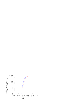
Figure 3: Percentage of the colour singlet contribution to the $\chi_{J}\longrightarrow p\bar{p}$ decay width that comes from region of values of $\alpha_{s}$ below some critical cutoff value $\alpha_{s}^{\mbox{\sevenrm crit.}}$. The solid and dot-dashed line are for $\chi_{1}$ and $\chi_{2}$, respectively. This shows that the bulk of the contributions in fact comes from $\alpha_{s}<0.6$ region.

Our results are shown in Table 3 together with the experimental measurements from Particle Data Group (PDG) [29] and the more recent BES Collaboration [30]. The errors associated with the PDG results are shown but those associated with BES are not because they are too large. One can consult them in ref. [30]. The results reveal a large discrepancy between the colour singlet contributions and the experimental widths. Before drawing any definite conclusions from these results, we first show that our calculation within MHSA is perturbatively consistent. To do that, an artificial cutoff $\alpha_{s}^{\mbox{\sevenrm crit.}}$ in the value of the coupling was introduced so that the integrations in Eq. (24) include only regions where $\prod^{3}_{i=1}\alpha_{s}(t_{i})<(\alpha_{s}^{\mbox{\sevenrm crit.}})^{3}$ was true. The value of $\alpha_{s}^{\mbox{\sevenrm crit.}}$ was varied to determine how much of the final results came from hard regions. The percentage of the final widths are plotted against $\alpha_{s}^{\mbox{\sevenrm crit.}}$ in Fig. 3 for both $J=1$ and $J=2$ charmonium. It shows clearly that by far the main contributions come from hard regions in which $\alpha_{s}$ remains below 0.6. So the Sudakov factor performed as expected to keep the soft non-perturbative region under control and suppressed.

To assess the uncertainties in the results, we have used the freedom from the uncertainty of the relation between $R_{p}^{\prime}(0)$ and $m_{c}$ from fit to charmonium parameters [31] and from quarkonium potential model [32] and also the value of $\Lambda_{\rm{QCD}}$ to maximize our results to see if they can be raised up to the experimental results. We found that they maximized with values of $R_{p}^{\prime}(0)=$ 0.194 GeV^5/2 and $m_{c}=$ 1.35 GeV and a larger $\Lambda_{\rm{QCD}}=$ 0.25 GeV. The colour singlet contribution to the decay width $\Gamma^{(1)}$ remains for $J=1$, 5–9 times and for $J=2$, 2–4 times below the measured results. At this point, one may wonder that the uncertainties of the proton distribution amplitude or wavefunction may make up for the remaining difference. As we have already discussed above, many proton wavefunctions derived from QCD sum rules do not work at our present scale of interest. For this very reason, the particular one we used here was constructed phenomenologically. Thus the apparent many choices of wavefunction and the fact that using each and everyone of them may lead to very different results are illusionary. One simply cannot use these other wavefunctions for $\chi_{J}$ decays. As to the nucleon decay constant, other values do exist from QCD sum rules or from lattice. For example, the values from QCD sum rules is about $5.0\times 10^{-3}$ GeV² [12, 21] or from lattice QCD there exist the two values $2.9$ or $6.6\times 10^{-3}$ GeV² [27]. Note that these are all smaller than ours, so using them will give even smaller results for the singlet contribution and not larger. The large experimental discrepancy of the data between PDG and BES cannot be explained but assuming that the true widths are somewhere in between or even near the BES results, it is clear that the colour singlet contribution alone cannot account for the experimental partial decay widths in agreement with our theoretical arguments presented in Sec. 3 and 4.

6 Combining Colour Singlet and Octet Contribution in the Standard Hard Scattering Approach

In the last section, we have shown that colour singlet contribution is not enough to account for the experimental measurements contradicting all earlier similar calculations done before the emergence of the colour octet state in P-wave charmonium and the associated improved understanding of the role of the higher Fock state of the quarkonium. It remains to show that the colour singlet and octet combination do indeed provide reasonable agreement to experimental data. We will outline the method of dealing with the colour octet and describe our calculations. The combined results will be shown but the details are given elsewhere [19].

The colour singlet calculation above was performed within the MHSA because of the two already mentioned advantages. The drawback of this scheme is, however, that it is more complicated to do a calculation. One has to include full wavefunctions and not only the distribution amplitudes. This means internal transverse momenta have to be kept in the hard perturbative part $T_{H}$. For the colour singlet contribution to $\chi_{J}$ decay, this proves to be manageable. We have seen the transverse separation space version of $T_{H}$ in Eq. (23). It contains several hyper-geometric functions and is therefore non-trivial. In the case of the colour octet, we will see presently that the calculation involves many more diagrams. In addition, proton and antiproton each carries three valence quarks. All these add up to the dimensions of the numerical integrations and complicate the calculation much more. The previous calculation was done within the MHSA to avoid the ambiguity of having to choose a renormalization scale by hand for $\alpha_{s}$ since the decay widths depend on the sixth power of the coupling $\alpha_{s}^{6}$ which leaves too much freedom or there is a lack of constraint to arrive at results that agree with data. In view of the complexity of MHSA, we will keep the calculation simple and avoid tangling ourselves in MHSA in the high dimensional computations by retreating back to the SHSA. This will, of course, bring back all the shortcomings of the SHSA but in spite of these, the SHSA can often be used to make a reasonable first estimate of the results.

As is now well known, the colour octet state of a P-wave charmonium includes, in addition to the usual $c\bar{c}$, a constituent gluon. The presence of this in the initial state requires it to be properly “put away” in the final hadrons in order not to have a net colour. This colour neutralization can be achieved in two different ways. The first is to allow this gluon to enter directly into or be a constituent in the final wavefunction of one of the outgoing hadrons. An example is shown in Fig. 4 (a). SHSA requires that no participant in the hard interaction to be disconnected from the rest as a consequence of the collinear approximation in SHSA. That is all constituents of any hadrons, be they part of an incoming or outgoing hadron, must be almost collinear. Therefore the connectedness of the constituents will ensure the even distribution of the hard momenta amongst the final constituents. The alternative is to let the constituent gluon be part of the hard perturbative part, that is to let it enter and end in $T_{H}$. Fig. 4 (b) shows this alternative. Comparing Fig. 4 (a) and (b), it is clear that the first is down by $1/M_{\chi_{J}}$ assuming hard momenta run through all connecting lines in $T_{H}$ as is usual in SHSA. Moreover, by including a higher Fock state in one of the outgoing hadrons will lead to extra suppression due to the smaller probability of that state, not to mention the undesirable involvement of further unknown wavefunction. The second possibility will be our choice for colour neutralization in the rest of this paper.

Figure 4: Example of two ways to achieve colour neutralization: (a) the constituent gluon enters the nucleon as part of the constituent in the nucleon after exchanging a gluon with the other constituents, (b) this gluon ends in the perturbative hard part $T_{H}$.

Figure 5: Example of $c\bar{c}$ annihilates through (a) one and (b) two gluons. Graph (a) is impossible in the colour singlet contribution.

As we mentioned earlier, C-parity only permits the $c\bar{c}$ to annihilate through two gluons in the colour singlet contribution. On the contrary in the colour octet, the very presence of a constituent gluon in the initial state enables many more possibilities. The heavy quark-antiquark pair, which is now protected from the C-parity constraint by the constituent gluon, can annihilate through one, two and three gluons. Fig. 4 (b) is an example of the latter and Fig. 5 (a) and (b) show a one-gluon and a two-gluon possibility, respectively. Fig. 5 (a) and Fig. 4 (b) are not permitted in the singlet case. In all, the graphs can be divided into ten groups based on ten basic graphs from which the members of each group can be constructed. These basic graphs are shown in Fig. 6. The four graphs in Fig. 2 are in fact counted as one basic graph of group (3) since they are related by symmetry. The members of all groups are generated by using the afore-mentioned colour neutralization method. That is to let the constituent gluon end in all possible allowed position on the basic graph as part of $T_{H}$. This generates between four to eleven graphs depending on the group. For example, Fig. 4 (b) is generated from group (5) by adding a gluon emerging from the $\chi_{J}$ and ending on one of the light quark lines, Fig. 5 (a) is from group (10) and Fig. 5 (b) is from group (4) of Fig. 6. The latter two are generated by letting the constituent gluon to end on the three-gluon vertex on the group (10) and (4) basic graph, respectively. More details on these are given elsewhere [19].

Figure 6: The feynman graphs that represent the ten basic groups from which the graphs of the colour octet contributions are generated. Each graph is assigned a group number as indicated.

The decay amplitude has the form of Eq. (3). The convolution now involves only distribution amplitudes. That of the proton is shown in Sec. 5. The relevant part is obtained by going to transverse position ${b}$-space and setting ${b}=0$ in the wavefunction or equivalently one can integrate out the transverse momenta ${{k}_{\perp}}$ in momentum space as shown in Eq. (4). The other distribution amplitudes or wavefunctions that we need is the colour octet of the $\chi_{J}$. These have to be constructed because the importance of the colour octet in exclusive reactions has not been realized up to now. For $\chi_{J}$ charmonia with momentum $P$, these can be expressed as

$$|\chi_{\chi_{J}}^{(8)},P\rangle\,=\,\frac{t^{a}_{c\bar{c}}}{2}\,f_{\chi_{J}}^{(8)}\,\int[\mbox{d}z]\phi_{\chi_{J}}^{(8)}(z_{1},z_{2},z_{3})\,S_{J\nu}^{(8)}(P)\;|c\bar{c}g;P\rangle$$ (27)

where $S_{J\nu}^{(8)}(P)$ is the spin-wavefunction [17, 19]. It is most convenient to use a product of delta functions for the distribution amplitude $\phi_{\chi_{J}}^{(8)}(z_{1},z_{2},z_{3})$ to set $z=0.15$ for the constituent gluon and dividing the remaining momentum fractions $z_{1}=z_{2}=(1-z)/2$ for the heavy quarks. This value of $z$ was found to be most appropriate in [17] and the decay constant $f_{\chi_{2}}^{(8)}=0.90\times 10^{-3}$ GeV² was fitted from $\chi_{2}\longrightarrow\pi\pi$. The same decay mode is not permitted for $\chi_{1}$ and the value of $f^{(8)}_{\chi_{1}}$ is therefore unconstrained but it is expected to be of the same order. We found a somewhat smaller value at $f^{(8)}_{\chi_{1}}=0.225\times 10^{-3}$ GeV² for $\chi_{1}$ from the decay into $p\bar{p}$.

The hard part $T_{H}$ of the singlet contribution is essentially the ${b}={b}^{\prime}=0$ version of Eq. (23) whereas that of the octet contribution now comes from an evaluation and summation over all members of the ten contributing groups. More explicitly the octet hard perturbative part can be written as

$$\{T^{J\;(8)}_{H}(x,y)\}_{\lambda_{1},\lambda_{2},\lambda_{3}} = i\;(4\pi\alpha_{s}(m_{c}))^{3}\sqrt{4\pi\alpha^{soft}_{s}}\;(2m_{c})^{7}$$

$$\times\sum_{{g\in Groups}\atop{m\in Members}}S_{g}P_{g\,m}(x,y)\{N^{J}_{g\,m}(x,y)\}_{\lambda_{1},\lambda_{2},\lambda_{3}}\;,$$

where $P_{g\,m}(x,y)$ is the product of propagators of the member $m$ graph of group $g$ and $S_{g}$ is a symmetry factor of group $g$ to take care of similar potential groups that are related to this group by simple change of variables. The $\{N^{J}_{g\,m}(x,y)\}_{\lambda_{1},\lambda_{2},\lambda_{3}}$ contains the light constituent quark helicity dependence of the outgoing nucleon and it denotes the numerator of this member $m$ graph. The convolution of $T_{H}$ with the distribution amplitudes can be expressed in the form of decay form factors for the octet contributions

$${\cal B}_{J}^{p\;(8)} = \sum_{\lambda_{1},\lambda_{2},\lambda_{3}=\pm}{{f^{(8)}_{\chi_{J}}\;\sigma_{J}}\over{2m_{c}\;(4m_{c})^{4}}}\int[\mbox{d}x][\mbox{d}y]\;\{T^{J\;(8)}_{H}(x,y)\}_{\lambda_{1},\lambda_{2},\lambda_{3}}\;\|\hat{\Psi}^{p}(x,0)\hat{\Psi}^{p}(y,0)\|_{\lambda_{1},\lambda_{2},\lambda_{3}}\;,$$

where $\sigma_{1}=1/\sqrt{2}$ and $\sigma_{2}=1$ as given below Eq. (24), and the product of proton wavefunction factor $\|\hat{\Psi}^{p}\hat{\Psi}^{p}\|_{\lambda_{1},\lambda_{2},\lambda_{3}}$ is similar in form to the wavefunction factor enclosed within braces in Eq. (24) but this one has helicity dependence and is evaluated at ${b}={b}^{\prime}=0$.

The hard part $T^{J}_{H}$ of individual feynman diagrams can be readily calculated using the usual feynman rules and the gauge choice by the same name. For example, the numerators and propagator denominators of our example member graphs shown in Fig. 4 (b), Fig. 5 (a) and (b) for some chosen helicity combinations are

$$P_{5,{\mbox{\sevenrm Fig.~{}\ref{f:col_neu} (b)}}}(x,y)\{N^{J}_{5,{\mbox{\sevenrm Fig.~{}\ref{f:col_neu} (b)}}}(x,y)\}_{-++} = (-1)^{J}\frac{\sqrt{2}}{6}\frac{z\{1-2x_{2}-4(x_{1}+x_{2}-z_{1})(y_{1}-z_{1})\}}{\{(z_{1}-x_{1})(z_{1}-y_{1})-1/4\}(2m_{c})^{2}}$$

$$\times\!\!\!\! \frac{1}{\{(z_{2}+z-x_{3})(z_{2}+z-y_{3})-1/4\}(2m_{c})^{2}}\;$$

$$\times\!\!\!\! \frac{1}{x_{1}y_{1}(2m_{c})^{2}}\;\frac{1}{x_{2}y_{2}(2m_{c})^{2}}\frac{1}{z(x_{3}-z)(2m_{c})^{2}}$$

$$\times\!\!\!\! \frac{1}{(x_{3}-z)(y_{3}-z)(2m_{c})^{2}+\rho^{2}}\;,$$ (30)

$$P_{10,{\mbox{\sevenrm Fig.~{}\ref{f:ot_g} (a)}}}(x,y)\{N^{J}_{10,{\mbox{\sevenrm Fig.~{}\ref{f:ot_g} (a)}}}(x,y)\}_{+\pm\mp} = \frac{\sqrt{2}\{2(1-z)-(-1)^{J}(y_{2}+y_{3}-z)\}}{(1-x_{1}-z)(1-y_{1}-z)(2m_{c})^{2}+\rho^{2}}$$

$$\times\!\!\!\! \frac{1}{(1-z)^{2}(2m_{c})^{2}}\;\frac{1}{(1-z)(1-y_{1}-z)(2m_{c})^{2}}$$

$$\times\!\!\!\! \frac{1}{x_{2}y_{2}(2m_{c})^{2}}\;\frac{1}{x_{3}y_{3}(2m_{c})^{2}}\;\frac{1}{(2m_{c})^{2}}\;,$$ (31)

and

$$P_{4,{\mbox{\sevenrm Fig.~{}\ref{f:ot_g} (b)}}}(x,y)\{N^{J}_{4,{\mbox{\sevenrm Fig.~{}\ref{f:ot_g} (b)}}}(x,y)\}_{+-+} = -\frac{5\sqrt{2}}{3}\frac{(-1)^{J}(x_{2}-y_{2})}{(1-x_{2}-z)(1-y_{2}-z)(2m_{c})^{2}+\rho^{2}}$$

$$\times\!\!\!\! \frac{1}{\{(z_{2}-x_{2})(z_{2}-y_{2})-1/4\}(2m_{c})^{2}}\frac{1}{x_{1}y_{1}(2m_{c})^{2}}$$

$$\times\!\!\!\! \frac{1}{x_{2}y_{2}(2m_{c})^{2}}\;\frac{1}{x_{3}y_{3}(2m_{c})^{2}}\;\frac{1}{(2m_{c})^{2}}\;,$$ (32)

respectively. To save on typing, we dropped $+i\epsilon$ in the propagators but its presence should be implicitly understood. The $\rho^{2}$ in some of the denominators above does not come with the propagators but has been inserted by hand. The purpose of this will be explained below. The explicit values of $S_{g}$ and the form of all other $P_{g\,m}(x,y)$, $\{N^{J}_{g\,m}(x,y)\}_{\lambda_{1},\lambda_{2},\lambda_{3}}$ and $\|\hat{\Psi}^{p}\hat{\Psi}^{p}\|_{\lambda_{1},\lambda_{2},\lambda_{3}}$ can be found in [19].

The above expressions are merely those of three example graphs. The full calculation is tedious but fortunately all necessary algebra can be handled by computer. Our treatment and method of dealing with the colour octet contribution are largely based on and parallel to those in [17, 18] and the various parameters obtained there are used in the present calculations. In particular $\alpha_{s}$ is set at the usual scale $m_{c}$ and in any case it is tied to the fitted octet decay constant of $\chi_{J}^{(8)}$, and it was assumed $\alpha_{s}^{\mbox{\sevenrm soft}}=\pi$ for this special coupling of the constituent gluon to the perturbative part as in [17]. This coupling is supposed to be softer than the others and therefore requires special treatment. Since the factors $f^{(8)}_{\chi_{J}}\sqrt{\alpha_{s}^{\mbox{\sevenrm soft}}}$ always appear together both in $\chi_{J}\longrightarrow\pi\pi$ and the present $\chi_{J}\longrightarrow p\bar{p}$, the detail of each individual factor is therefore less important than the combination. If the calculation were done within MHSA, both $\alpha_{s}^{\mbox{\sevenrm soft}}$ and its value need not be worried. The latter would be fixed dynamically. Once the constituent gluon has been dealt with and put into the perturbative hard part, the calculation itself is essentially the same as other calculations using SHSA scheme. One calculates $T_{H}$ perturbatively from all contributing graphs and then convolutes it with the distribution amplitudes of the hadron involved to get the probability amplitude.

We now return to the $\rho^{2}$ in Eqs. (30), (31) and (32) above. The purpose of inserting $\rho^{2}$ is to prevent two poles within one propagator from occurring simultaneously which is possible in the convolution integral in Eq. (LABEL:eq:o_df). When that happens, the $i\epsilon$ prescription cannot handle such singularities. For the expression in Eq. (30) the problem occurs when $x_{3}=y_{3}=z$ and for Eqs. (31) and (32) this is at $x_{1}=y_{1}=1-z$ and $x_{2}=y_{2}=1-z$, respectively. The presence of $\rho^{2}$ removes this kind of singularities in the integral. The reason that they are there is because of the collinear approximation of SHSA. Within this approximation, the hadron internal transverse momentum dependence of the perturbative hard part is dropped $T_{H}(x,y,{{k}_{\perp}})\longrightarrow T_{H}(x,y)$ in favor of hard momenta running through the internal lines of the relevant feynman graphs. As a consequence, they are dropped from the denominators of the propagators as well under the assumption that the large virtualities of the virtual propagating particles dwarf any such dependence. Had we relinquished our hold of the collinear approximation and calculated within the MHSA, such singularities simply do not exist. In the MHSA scheme, the internal transverse momenta of the hadrons involved are kept everywhere and they therefore serve as a natural cutoff of such singularities. From this example, the use of $\rho^{2}=\langle{{k}_{\perp}}^{2}\rangle$, the average transverse momentum square of the nucleon, as a regulator of these singularities naturally suggested itself. Although this treatment is somewhat ad hoc within SHSA, it is nevertheless practical and indeed has been used in [17].

Next there is the issue of gauge invariance. The common way of expressing hadron wavefunctions in terms of distribution amplitudes means that the energy-momentum of the hadron must be divided into portions and assigned to its partonic constituents. In the case of charmonium in a colour octet, the energy-momentum is therefore assigned as $P=P_{c}+P_{\bar{c}}+P_{g}$ with $P_{c}=z_{1}P$, $P_{\bar{c}}=z_{2}P$ and $P_{g}=zP$. Since $z_{1}=z_{2}$ the mass of the constituent heavy quark is then $z_{1}M_{\chi_{J}}\simeq z_{1}(2m_{c})$ whereas feynman rules do not take into account of particles existing in a bounded, confined state and therefore give the standard heavy fermion propagator $1/(\gamma\cdot P_{c}-m_{c})$ with the usual heavy quark mass $m_{c}$. Remembering that the probability amplitude of an interaction is only gauge invariant, after all feynman graphs of a given order have been included, provided that the external particles are all on their respective mass-shells. The conflict of $z_{1}(2m_{c})\not=m_{c}$ thus becomes a source for the violation of gauge invariance. This only arises in the graphs of group (3), (4) and (5). If one checks for gauge invariance, after many cancellations, the few remaining gauge violating terms are all proportional to $(1-2z_{1})m_{c}=zm_{c}$ as expected. Combining with other factors, these terms first enter at ${\cal O}(z^{3})$ in the numerators. Our calculations are therefore gauge invariant up to ${\cal O}(z^{2})$. As mentioned in [18], one could choose to make the results completely gauge invariant by using $(1-z)m_{c}$ in the propagator instead of $m_{c}$ but because of $z=0.15$, these gauge-invariance violating contributions are small and therefore do not worry us too much.

Our results are shown in Table 4. The colour singlet-octet combined results are given along with those from the singlet alone. The singlet results here differ from those in Table 3 because of the somewhat different values of the octet decay constants and the different treatments of the coupling and details between the two calculational schemes. But we are satisfied by the fact that the results are of the same order of magnitude. For experimental errors, the readers can consult ref. [30] and for theoretical ones, they will not be presented at this stage since they are tied closely to the experimental ones because the octet decay constants were obtained in [17, 18] by the requirement of a reasonable agreement with two different sets of experimental measurements. As mentioned before, the disagreement in the measurements between PDG and BES collaboration forces us to settle around the average of the two sets of results. This is also the case for the decay mode $\chi_{J}\longrightarrow\pi\pi$. Once a better agreement amongst the experiments is reached, the decay constants will have to be adjusted accordingly and estimates of theoretical errors be made.

As we mentioned already in Sec. 5, in the case that the true values are close to either the PDG or the BES set. Colour singlet alone cannot account for the measured decay widths. We have outlined and described our method to include the colour octet. As can be seen from above, with the colour octet contribution the theoretical situation is in a much better shape. Note that the $\chi_{J}$ singlet wavefunction is well known and in the MHSA, there is no free parameter in the calculation. As to the colour octet wavefunction, that of the $\chi_{2}$ is completely fixed by $\chi_{2}\longrightarrow\pi\pi$ and therefore there is no remaining freedom left in $\chi_{2}\longrightarrow p\bar{p}$. The value of $f^{(8)}_{\chi_{1}}$ although cannot be fixed by the pseudo-scalar decay mode like the $\chi_{2}$, the smaller but still at the same order value as that of the $\chi_{2}$ can be viewed as a consistent result. Since $\chi_{1}$ is a somewhat different P-wave charmonium from its even spin partners, one is not too surprising that the result is as it is.

Before summarizing, we would like to address the issue of the validity of our perturbative calculations. Although the charmonium mass $M_{\chi_{J}}\simeq$ 3.5 GeV is not extremely large, the scales of the coupling are set essentially by the virtualities of the intermediate gluons and not, for example, by the energies of the final partons. For annihilation into three gluons, each gluon will have about 1.1 GeV and even with a large value for $\Lambda_{\rm{QCD}}=$ 0.25 GeV, the coupling will be about $\alpha_{s}=$ 0.508. It is not too bad for a perturbative calculation. On the other hand, if one compares the combined colour singlet and octet results in Table 4 with those of the colour singlet alone in Table 3, one might be alarmed with the apparently large combined results when compared to the smaller singlet results and start questioning the validity of the perturbative calculations. First, to compare the singlet widths with the combined singlet and octet widths directly is misleading. A more proper comparison is between the singlet amplitudes with the combined amplitudes or equivalently one compares the square root of the widths. If this is done, it can be established that the combined amplitudes are only a factor of 4.5 for $\chi_{1}$ and 3.0 for $\chi_{2}$ larger than the corresponding singlet ones, so the octet parts are nowhere near completely dominating the results. On the contrary, both the singlet and octet parts contribute comparably to the final results. Second, with proton-antiproton in the final states and not pions as in [17], one might worry about getting too close to the boundary of the perturbative region. Fortunately, the calculation of the colour singlet contribution in Sec. 5 and of $J/\psi$ decay into baryon-antibaryon pair in ref. [33] both within the MHSA showed that the bulk of the contribution came not from large coupling non-perturbative region. This should serve as an example of even with a pair of baryons in the final states, the calculational scheme of SHSA and MHSA are still under perturbative control and can be used self-consistently. Third, although it is not possible to do a full calculation in the MHSA, not all ten groups of Feynman diagrams in the colour octet contribution lead to unmanageably high dimensional integrations. For those that can be calculated numerically with sufficient accuracy, we have checked that the bulk of the contributions did indeed come from smaller values of the coupling below $\alpha_{s}=$ 0.5. Using a cutoff of $\alpha_{s}^{\mbox{\sevenrm cutoff}}=$ 0.5, well over 50 % of the contributions were included and with $\alpha_{s}^{\mbox{\sevenrm cutoff}}=$ 0.6, 98 % were included. Of course, we have not confirmed reasonable widths within the MHSA due to the complexity of the calculations and the limitation of present days computing power, but this should still serve to demonstrate to a certain extent that the theoretical arguments presented above are reasonably sound and that the calculational schemes used are self-consistent.

To summarize, we have provided arguments in support of the inclusion of colour octet in P-wave charmonium decay and by explicit calculation, have shown that although the same infrared divergence in inclusive decay does not exist in exclusive process, for consistency this next higher Fock state of the P-wave charmonium must still be included. With that, the would-be contradiction discussed at the end of Sec. 2 is resolved. The applicability of our arguments is obviously not restricted only to charmonia. In fact, they are true and should work even better for heavier quarkonia such as $b\bar{b}$.

Figure Captions

• The leading decay process for (a) $\chi_{0}$ and $\chi_{2}$ and (b) $\chi_{1}$. A possible decay of the higher Fock state, the colour octet, of the $\chi_{J}$ is shown in (c). In the infrared limit of the outgoing gluon, (b) and (c) are degenerate.

• Feynman graphs for the colour singlet $\chi_{J}$ decay into proton-antiproton.

• Percentage of the colour singlet contribution to the $\chi_{J}\longrightarrow p\bar{p}$ decay width that comes from region of values of $\alpha_{s}$ below some critical cutoff value $\alpha_{s}^{\mbox{\sevenrm crit.}}$. The solid and dot-dashed line are for $\chi_{1}$ and $\chi_{2}$, respectively. This shows that the bulk of the contributions in fact comes from $\alpha_{s}<0.6$ region.

• Example of two ways to achieve colour neutralization: (a) the constituent gluon enters the nucleon as part of the constituent in the nucleon after exchanging a gluon with the other constituents, (b) this gluon ends in the perturbative hard part $T_{H}$.

• Example of $c\bar{c}$ annihilates through (a) one and (b) two gluons. Graph (a) is impossible in the colour singlet contribution.

• The feynman graphs that represent the ten basic groups from which the graphs of the colour octet contributions are generated. Each graph is assigned a group number as indicated.

Table Captions

• The mass dimensions of the decay constants of the hadrons discussed in the text. They can be deduced from Eqs. (4) and (5).

• The make-up of the parity ${\cal P}$ and C-parity ${\cal C}$ of each colour singlet and octet state of the $J/\psi$ and $\chi_{J}$ for states with up to three constituents.

• Comparing colour singlet contribution of $\chi_{J}$ decay into $p\bar{p}$ to the experimental data.

• The colour singlet and octet combined partial decay width within the SHSA of $\chi_{J}$ decay into proton-antiproton. Experimental measurements are also shown for comparison.

Tables

Table 1: The mass dimensions of the decay constants of the hadrons discussed in the text. They can be deduced from Eqs. (4) and (5).

Hadron	No. of	Total Orbital Angular	Mass dimension
	Constituents	Momentum $L$	of $f$ [$f$]
$\pi$, $K$	2	0	1
$J/\psi^{(1)}$	2	0	1
$\chi^{(1)}_{J}$	2	1	2
$p$, $\bar{p}$	3	0	2
$J/\psi^{(8)}$	3	1	3
$\chi^{(8)}_{J}$	3	0	2

Table 2: The make-up of the parity ${\cal P}$ and C-parity ${\cal C}$ of each colour singlet and octet state of the $J/\psi$ and $\chi_{J}$ for states with up to three constituents.

Hadron	$L^{c}_{\bar{c}}$	$S_{c\bar{c}}$	$L^{c\bar{c}}_{g}$	$N_{g}$	${\cal P}=(-1)^{N_{g}+L^{c}_{\bar{c}}+L^{c\bar{c}}_{g}+1}$	${\cal C}=(-1)^{N_{g}+S_{c\bar{c}}+L^{c}_{\bar{c}}}$
($c\bar{c}$ state)
$J/\psi^{(1)}$ (${}^{3}S_{1}$)	0	1	0	0	-1	-1
$J/\psi^{(8)}$ (${}^{3}P_{J}$)	1	1	0	1	-1	-1
$J/\psi^{(8)}$ (${}^{1}S_{0}$)	0	0	1	1	-1	-1
$J/\psi^{(8)}$ (${}^{3}S_{1}$)?	0	1	0	1	+1?	+1?
$J/\psi^{(8)}$ (${}^{3}S_{1}$)?	0	1	1	1	-1	+1?
$\chi_{J}^{(1)}$ (${}^{3}P_{J}$)	1	1	0	0	+1	+1
$\chi_{J}^{(8)}$ (${}^{3}S_{1}$)	0	1	0	1	+1	+1

Table 3: Comparing colour singlet contribution of $\chi_{J}$ decay into $p\bar{p}$ to the experimental data.

$J$	$\Gamma^{(1)}(\chi_{J}\rightarrow p\bar{p})$ (eV)	PDG (eV) [29]	BES (eV) [30]
1	2.53	75.68 $\pm$ 10.50	37.84
2	16.58	200.00 $\pm$ 20.00	118.00

Table 4: The colour singlet and octet combined partial decay width within the SHSA of $\chi_{J}$ decay into proton-antiproton. Experimental measurements are also shown for comparison.

	$\Gamma^{(1)}$ (eV)	$\Gamma^{(1)+(8)}$ (eV)	PDG (eV) [29]	BES (eV) [30]
$\chi_{1}\longrightarrow p\bar{p}$	3.15	56.27	75.68 $\pm$ 10.50	37.84
$\chi_{2}\longrightarrow p\bar{p}$	12.29	154.19	200.00 $\pm$ 20.00	118.00

References

- [1] S.J. Brodsky and G.P. Lepage, Phys. Rev. D 22 (1980) 2157.
- [2] J. Botts and G. Sterman, Nucl. Phys. B 325 (1989) 62.
- [3] H.N. Li and G. Sterman, Nucl. Phys. B 381 (1992) 129.
- [4] G.T. Bodwin, E. Braaten and G.P. Lepage, Phys. Rev. D 46 (1992) 1914.
- [5] G.T. Bodwin, E. Braaten and G.P. Lepage, Phys. Rev. D 51 (1995) 1125.
- [6] R. Barbieri, R. Gatto, and R. Kögerler, Phys. Lett. B 60 (1976) 183.
- [7] R. Barbieri, R. Gatto, and E. Remiddi, Phys. Lett. B 61 (1976) 465.
- [8] V.L. Chernyak and A.R. Zhitnitsky, Nucl. Phys. B 201 (1982) 492.
- [9] A. Andrikopoulou, Z. Phys. C 22 (1984) 63.
- [10] P.H. Damgaard, K. Tsokos and E.L. Berger, Nucl. Phys. B 259 (1985) 285.
- [11] V.L. Chernyak, A.A. Ogloblin and A.R. Zhitnitsky, Z. Phys. C 42 (1989) 583.
- [12] F. Murgia and M. Melis, Phys. Rev. D 51 (1995) 3487.
- [13] M. Beneke and I.Z. Rothstein, Phys. Rev. D 54 (1996) 2005.
- [14] E. Braaten and Y.-Q. Chen, Phys. Rev. D 54 (1996) 3216.
- [15] S. Fleming and I. Maksymyk, Phys. Rev. D 54 (1996) 3608.
- [16] W.-K. Tang and M. Vänttinen, Phys. Rev. D 54 (1996) 4349.
- [17] J. Bolz, P. Kroll and G.A. Schuler, Phys. Lett. B 392 (1997) 198.
- [18] J. Bolz, P. Kroll and G.A. Schuler, Eur. Phys. J. C 2 (1998) 705.
- [19] S.M.H. Wong, preprint NUC-MINN-98/12-T, hep-ph/9903236, to appear in Eur. Phys. J. C.
- [20] V.L. Chernyak and A.R. Zhitnitsky, Phys. Rep. 112 (1984) 173.
- [21] V.L. Chernyak, A.A. Ogloblin and A.R. Zhitnitsky, Z. Phys. C 42 (1989) 569.
- [22] M. Gari and N.G. Stefanis, Phys. Rev. D 35 (1987) 1074.
- [23] I.D. King and C.T. Sachrajda, Nucl. Phys. B 279 (1987) 785.
- [24] M. Bergmann and N.G. Stefanis, Phys. Rev. D 47 (1993) 3685.
- [25] A.V. Radyushkin, Nucl. Phys. A 532 (1991) 141.
- [26] J. Bolz, R. Jakob, P. Kroll, M. Bergmann and N.G. Stefanis, Z. Phys. C 66 (1995) 267.
- [27] J. Bolz and P. Kroll, Z. Phys. A 356 (1996) 327.
- [28] V.A. Novikov, L.B. Okun, M.A. Shifman, A.I. Vainshtein, M.B. Woloshin and V.I. Zakharov, Phys. Rep. 41 (1978) 1.
- [29] R.M. Barnett et al, Phys. Rev. D 54 (1996) 1.
- [30] J.Z. Bai et al, BES Collaboration, Phys. Rev. Lett. 81 (1998) 3091.
- [31] M.L. Mangano and A. Petrelli, Phys. Lett. B 352 (1995) 445.
- [32] C. Quigg and J.L. Rosner, Phys. Rep. 56 (1979) 167.
- [33] J. Bolz and P. Kroll, Eur. Phys. J. C 2 (1998) 545.