Praca

The Pennsylvania State University

The Graduate School

Eberly College of Science

EXCLUSIVE, HARD DIFFRACTION IN QCD

A Thesis in

Physics

by

Andreas Freund

Submitted in Partial Fulfillment

of the Requirements

for the Degree of

Doctor of Philosophy

August 1998

Abstract

In the first chapter we give an introduction to hard diffractive scattering in QCD to introduce basic concepts and terminology, thus setting the stage for the following chapters.

In the second chapter we make predictions for nondiagonal parton distributions in a proton in the LLA. We calculate the DGLAP-type evolution kernels in the LLA, solve the nondiagonal GLAP evolution equations with a modified version of the CTEQ-package and comment on the range of applicability of the LLA in the asymmetric regime. We show that the nondiagonal gluon distribution $g(x_{1},x_{2},t,\mu^{2})$ can be well approximated at small $x$ by the conventional gluon density $xG(x,\mu^{2})$.

In the third chapter, we discuss the algorithms used in the LO evolution program for nondiagonal parton distributions in the DGLAP region and discuss the stability of the code. Furthermore, we demonstrate that we can reproduce the case of the LO diagonal evolution within less than $0.5\%$ of the original code as developed by the CTEQ-collaboration.

In chapter 4, we show that factorization holds for the deeply virtual Compton scattering amplitude in QCD, up to power suppressed terms, to all orders in perturbation theory. Furthermore, we show that the virtuality of the produced photon does not influence the general theorem.

In chapter 5, we demonstrate that perturbative QCD allows one to calculate the absolute cross section of diffractive exclusive production of photons at large $Q^{2}$ at HERA, while the aligned jet model allows one to estimate the cross section for intermediate $Q^{2}\sim 2GeV^{2}$. Furthermore, we find that the imaginary part of the amplitude for the production of real photons is larger than the imaginary part of the corresponding DIS amplitude, leading to predictions of a significant counting rate for the current generation of experiments at HERA. We also find a large azimuthal angle asymmetry in $ep$ scattering for HERA kinematics which allows one to directly measure the real part of the DVCS amplitude and hence the nondiagonal parton distributions.

In the last chapter, we propose a new methodology of gaining shape fits to nondiagonal parton distributions and, for the first time, to determine the ratio $\eta$ of the real to imaginary part of the DIS amplitude. We do this by using several recent fits to $F_{2}(x,Q^{2})$ to compute the asymmetry $A$ for the combined DVCS and Bethe-Heitler cross section. The asymmetry $A$, isolates the interference term of DVCS and Bethe-Heitler in the total cross section, in other words, by isolating the real part of the DVCS amplitude through this asymmetry one has access to the nondiagonal parton distributions for the first time. Comparing the predictions for $A$ against experiment would allow one to make a prediction of the shape, though not absolute value, of nondiagonal parton distributions.

In the appendix, to illustrate an application of distributional methods as discussed in chapter 4, we will show, with the aid of simple examples, how to make simple estimates of the sizes of higher-order Feynman graphs. Our methods enable appropriate values of renormalization and factorization scales to be made. They allow the diagnosis of the source of unusually large corrections that are in need of resummation.

Contents

1. List of Figures
2. 1 Introduction
   1. 1.1 What is Diffraction in QCD ?
   2. 1.2 Hard Diffraction in QCD
      1. 1.2.1 Theoretical Foundation
      2. 1.2.2 What kind of diffractive processes are calculable in QCD ?
3. 2 Nondiagonal Parton Distributions in the Leading Logarithmic Approximation
   1. 2.1 Introduction
   2. 2.2 Nondiagonal parton distributions and hard diffractive processes.
      1. 2.2.1 GLAP evolution equation for hard diffractive processes
      2. 2.2.2 Small $x_{i}$ behavior of the nondiagonal gluon distribution
   3. 2.3 Kernels in the LLA
   4. 2.4 Predictions for nondiagonal parton distributions
   5. 2.5 Limitations of the LLA in the nondiagonal case
   6. 2.6 Conclusions and Outlook
4. 3 Methods in the LO Evolution of Nondiagonal Parton Distributions: The DGLAP Case
   1. 3.1 Introduction
   2. 3.2 Review of Nondiagonal Parton Distributions, Evolution Equations and Kernels
      1. 3.2.1 Nondiagonal Parton Distributions
      2. 3.2.2 The GLAP-Evolution Equations for Nondiagonal Parton Distributions
   3. 3.3 Differences between the CTEQ and our Algorithms
      1. 3.3.1 NEWARRAY and NINTEGR
      2. 3.3.2 Modifications in NSRHSM, NSRHSP and SNRHS
   4. 3.4 Code Analysis
   5. 3.5 Conclusions
5. 4 Proof of Factorization for Deeply Virtual Compton Scattering in QCD
   1. 4.1 Introduction
   2. 4.2 Factorization Theorem
   3. 4.3 Proof of Theorem
      1. 4.3.1 Regions
      2. 4.3.2 Power Counting
      3. 4.3.3 Leading Regions
      4. 4.3.4 Proof of absence of a soft part in leading regions
      5. 4.3.5 Subtractions
      6. 4.3.6 Taylor expansion
      7. 4.3.7 Gauge Invariance
      8. 4.3.8 Partons with $k^{+}=0$: breakpoints and endpoints
      9. 4.3.9 Completion of Proof
   4. 4.4 Conclusion
6. 5 Diffractive Exclusive Photon Production in DIS at HERA
   1. 5.1 Introduction
   2. 5.2 The amplitude for diffractive virtual Compton scattering at intermediate $Q^{2}$
   3. 5.3 The amplitude for exclusive real photon production at large $Q^{2}$.
   4. 5.4 The t-slope of the $\gamma^{*}N\to\gamma N$ cross section
   5. 5.5 The rate of exclusive photon production at HERA
   6. 5.6 The complete cross section of exclusive photon production
      1. 5.6.1 t-dependence of Bethe-Heitler as compared to DVCS for different $Q^{2}$
      2. 5.6.2 DVCS alternative to tagged proton in the final state
   7. 5.7 Conclusions
7. 6 DVCS in DIS at HERA - A Probe of Asymptotia
   1. 6.1 Introduction
   2. 6.2 Relations between DVCS and DIS
   3. 6.3 The different fits to $F_{2}(x,Q^{2})$
   4. 6.4 Results for the asymmetry $A$
   5. 6.5 Conclusions
8. A Direct Estimation of Sizes of Higher-Order Graphs
   1. A.1 Introduction
   2. A.2 Euclidean self-energy in $\phi^{3}$ theory
      1. A.2.1 Renormalization
      2. A.2.2 Estimate
      3. A.2.3 Implication for QCD
   3. A.3 Wilson coefficient for deep-inelastic scattering
      1. A.3.1 Real gluon
      2. A.3.2 Sum of virtual and real graphs
      3. A.3.3 Estimate of size
      4. A.3.4 Interpretation
   4. A.4 More detailed estimation of $F_{T,L}$ to one-loop order
      1. A.4.1 Estimation of $F_{L}$
      2. A.4.2 Estimation of $F_{T}$
   5. A.5 The remaining longitudinal and transverse contributions to the Wilson coefficient
      1. A.5.1 Transverse part of the self-energy
      2. A.5.2 The transverse part of the ladder diagram
      3. A.5.3 Longitudinal part of the vertex correction, self-energy and ladder diagram
   6. A.6 Conclusions
9. Bibliography

List of Figures

lof.

Chapter 1 Introduction

1.1 What is Diffraction in QCD ?

The first question we will attempt to answer is: What is diffraction in QCD? The answer is, of course, not $42$ [2] but rather complicated and multi layered going to the heart of our understanding of QCD or lack thereof.

Before proceeding, we will introduce customary notation for variables used in describing inelastic and diffractive phenomena.

In the process

$$e(l)+p(p) \rightarrow e^{\prime}(l^{\prime})+X+P^{\prime}(p^{\prime})$$

or

$$p(l)+p(p) \rightarrow p(l^{\prime})+p(p^{\prime})$$

or

$$p(l)+p(p) \rightarrow X+p(p^{\prime})$$ (1.1)

with the momenta of the particles given in brackets. For defineteness and since this type of process will be of greatest relevance in the remainder of the thesis, we will introduce the relevant kinematics for the electron proton scattering. The center of mass energy squared is $s=(l+p)^{2}$ and the center of mass squared of the hadronic system is

$$W^{2}=(q+p)^{2}=-Q^{2}+2p\cdot q+m_{p}^{2}=Q^{2}\left(-1+\frac{1}{x}\right)+m_{p}^{2},$$ (1.2)

with $q=(-xp_{+},Q^{2}/2xp_{+},0_{\perp})$ being the four momentum of the virtual photon exchanged between the lepton and the rest of the system (see Fig. 1.1) and $Q^{2}=-q^{2}$. The Bjorken $x$ is defined as:

$$x_{bj}=\frac{Q^{2}}{2p\cdot q}$$ (1.3)

with $p$ being the four momentum of the incoming proton.

Figure 1.1: Typical lepton-proton scattering with a final state $X$ clearly separated from the final state proton with the exchanged object between the virtual photon and the proton denoted by a dashed line.

$ep$ scattering, but also the rest of the reactions in (1.1), is said to be in the diffractive region if $X$ is sufficiently separated from the final state proton; the precise meaning of this statement will be explained below. $X$ is used in diffractive interactions to denote the part of the final state which might be in the case of $ep$ scattering, a real photon, a vector meson or two jets. If the final state proton dissociates as well, we will denote this state by $Y$ to indicate that it is still separated from the state $X$. The kinematics are the following: The square of the momentum transfer at the proton vertex is

$$t=(p-p^{\prime})^{2}$$ (1.4)

where $p^{\prime}$ is the four momentum of the outgoing proton. In the case of dissociation of the final state proton the proton momentum $p^{\prime}$ should be replaced by the four momentum of the outgoing system $Y$. A fourth Lorentz scalar is needed to define the kinematics of the hadronic part of the final state.

The fraction of the proton momentum carried by the pomeron is

$$x_{P}=\frac{(p-p^{\prime})\cdot q}{p\cdot q}=\frac{M_{X}^{2}+Q^{2}-t}{W^{2}+Q^{2}-m_{p}^{2}}$$ (1.5)

where $M_{X}$ is the mass of the produced system. Note that the influence of $t$ and $m_{p}$ on $x_{P}$ is negligible for large $Q^{2}$ and $W^{2}$.

The rapidity of a particle in the final state is given by

$$y=\frac{1}{2}\ln\left(\frac{E+p_{z}}{E-p_{z}}\right).$$ (1.6)

Now consider the total hadronic cross section for processes like $pp,p\bar{p},\gamma p$, etc. as a function of the center of mass energy $\sqrt{s}$ [3]. Their total cross section can be described as

$$\sigma_{tot}^{h-h}=Ys^{-\eta}+Xs^{\epsilon}.$$ (1.7)

which is the form predicted by Regge theory. The first term describes the decrease of the cross section with $s$ at low energies and the second the slow increase at high energies. CDF [4], Cudell et al. [5] and originally Donnachie and Landshoff [6] performed a fit using different hadronic data in each case to determine the values of $\eta$ and $\epsilon$ and thus obtain a universal description of the hadronic cross section. $\eta$ was found to be around $0.45$, with the results for $\epsilon$ varying on the data used for the fit with $0.08$ from Donnachie and Landshoff to $0.112$ from CDF.

This behavior of the total cross section can be interpreted in terms of Regge theory [7]. The hadronic reaction $A+B\rightarrow C+D$ can be described by the $t$-channel exchange of a family of off-shell particles such that the relevant quantum numbers are conserved. There exists a theoretical relation between the spin $J$ and the mass squared ($t$) for these particles which has the the approximate form

$$J_{i}=\alpha_{i}(t)=\alpha_{i}(0)+\alpha_{i}^{\prime}t.$$ (1.8)

The particles lie on so-called “Regge trajectories”, with intercept $\alpha_{i}(0)$ and slope $\alpha_{i}^{\prime}$ where i stands for the different particles. The dependence of the elastic cross section with $t$ should behave as

$$\frac{d\sigma_{el}}{dt}\sim\left(\frac{s}{s_{0}}\right)^{2(\alpha_{1}(0)-1)}e^{bt},~{}~{}\mbox{with}~{}~{}b=b_{0}+2\alpha_{1}^{\prime}\ln\left(\frac{s}{s_{0}}\right).$$ (1.9)

The term in Eq. (1.7), dominant at low energies, was fitted in Ref. [6] and corresponds to the intercept $\alpha_{R}\simeq 0.5$ for reggeon exchange, i.e. , the degenerate $\rho,\omega,f$ and $a$ trajectories. The dominant term at high energies in Eq. (1.7) corresponds to the so-called pomeron trajectory (see Ref. [12]) with an intercept $\simeq 1.08$ according to the fit in [6]. The slope $\alpha_{P}^{\prime}$ was fitted to be $\simeq 0.25~{}\mbox{GeV}^{-2}$, implying that the exponential $t$ distribution becomes steeper with increasing energy.

The $d\sigma/dt$ distribution in p - p elastic scattering has a characteristic behavior with an exponential fall-off, a dip and a second exponential, which is reminiscent of the diffractive pattern of light by a circular aperture [8], hence the name Diffraction was used to indicate a pomeron exchange. Processes mediated by pomeron exchange can be classified as elastic, single diffractive and double diffractive as shown in Fig. 1.2. From Fig. 1.2, due to the lack of additional final state particles created through color interactions with the exchanged pomeron, it is also clear that the pomeron has to carry vacuum quantum numbers, i.e. , it has to be a color singlet and one expects to see a rapidity gap between the leading particle B and the system X.

Figure 1.2: a) elastic scattering. b) single diffractive scattering. c) double diffractive scattering.

The main open questions on the pomeron are: Does one have a universal “soft” pomeron or a continuum of different objects with different energy dependences etc. up to high energies ? Can it be treated as a particle with a partonic substructure [9] and if so what is the pomeron structure function? Does factorization hold or not?

In the following discussion on hard diffraction and the following chapters some of these questions will be addressed.

1.2 Hard Diffraction in QCD

Diffractive processes with one or several large scales, for example large $Q^{2}$ in deep-inelastic scattering (DIS), are called hard. Especially interesting are diffractive DIS processes at large $Q^{2}$ such as electro-production of longitudinally, polarized vector mesons and deeply virtual compton scattering (DVCS), which we will treat in more depth later, since they offer a unique opportunity to probe the interplay between soft and hard QCD physics. The fact that one observes a substantial number of diffractive like events at high $Q^{2}$ at the HERA, CDF and D0 experiments, is a signal for the interplay of hard and soft QCD phenomena. There are two effects which are expected to play an important role, color transparency for systems consisting of quarks and gluons contained within a small size configuration and color opacity for large size configurations. Small size configurations lead to reactions dominated by hard processes with a cross section rising with energy, while reactions of large size configurations are dominated by soft processes. In order to test QCD on a quantitative and qualitative level, the ability to separate these two regimes from one another becomes essential. In this context one can address the following issues:

• The dynamics of compact systems, color transparency and perturbative color opacity in hard diffractive processes like electro-production of longitudinally polarized vector mesons or DVCS.

• QCD predictions for the high momentum behavior of wave functions of hadrons consisting of light quarks and QCD physics of heavy quarkonia.

• Violation of the DGLAP evolution equation. Due to unitarity considerations the increase of parton densities at small $x$ will slow down and it is believed that this effect can be observed at HERA in hard diffractive processes, in the measurements of the proton structure functions at moderate $Q^{2}$, as well as in the measurements of the structure functions of nuclei.

• Semi-classical approximation to high energy interactions. In the limit of strong color fields which are typical in the HERA kinematical regime, new developments and tests of the semi-classical approach are possible [10].

1.2.1 Theoretical Foundation

In order to understand the issue of the interplay of soft and hard physics in high energy reactions let us quickly classify them according to the number of scales involved [11].

• Soft QCD: Soft hadron collisions are usually considered to be processes with a scale of $\sim 1$ fm. We have already discussed this topic in Sec. 1.1.

• Hard QCD evolution: This second class consists of hard processes which are determined by two or more different scales in the interaction. DIS as well as hard diffractive processes belong to this class. The hard scale is provided by the virtuality of the photon or jets whereas the soft scale is set by the size of the proton.

  In order to use pQCD one has to prove that the short distance part of the interaction factorizes from the soft one. This is achieved for the total cross section and special hard diffractive processes as for example diffractive vector meson production and DVCS [25, 47] by proving QCD factorization theorems. These factorization theorems lead to BL and DGLAP type equations [25, 47] describing the evolution from large $Q^{2}$ to the scale of soft QCD processes, hence the soft physics ( in particular the soft pomeron ) enters as boundary conditions to these equations.

  One has to mention that the characteristic attribute of two scale processes is the violation of the pomeron pole factorization, i.e. , the description of the energy dependence of diffractive processes by a universal trajectory as mentioned before in Sec. 1.1. Therefore one may observe different energy dependences for different external particles and the energy dependence may change with $Q^{2}$.

• BFKL Evolution: The original form of the BFKL equation was derived under the assumption of a small but fixed value of $\alpha_{s}$ with the scale of $\alpha_{s}$ set by the scale of the external particle. The BFKL approximation therefore applies to processes with one large scale. HERA would offer a clean test by measuring high-$p_{\perp}$ forward jets with $p_{\perp}^{2}\simeq Q^{2}$ in low $x$ DIS as suggested by A. Mueller [13]. In diffractive DIS, semi-inclusive diffractive vector production with large momentum transfer $t$ would be a place to look for the BFKL pomeron.

• Color Transparency and Perturbative Color Opacity: Color transparency is a phenomenon which describes within QCD the interaction of a small size, color neutral parton configuration with a hadronic target. The essence of color transparency is expressed by the following formula [14, 15, 71] which follows from the factorization theorem for hard processes in QCD:

  $$\sigma^{q\bar{q}}_{T}=2\alpha_{s}\pi^{2}\frac{1}{N_{c}}Tr\left(\frac{L^{2}}{8}\right)xG(x,9/b^{2}),$$ (1.10)

  where $L^{2}$ is the casimir operator of color $SU(3)$, b is the transverse separation between the $q\bar{q}$ system and G stands for the gluon distribution in the target.

  The name “Color Transparency” stems from the fact that high energy processes are dominated by gluon exchange and that the cross section for a small size configuration is, through the gluon distribution, indirectly related to its size in the impact parameter space. The decrease of the cross section with decreasing size is partly compensated by the known increase of the gluon density. Furthermore, at fixed b, the cross section increases with increasing energy. Also, the interaction cross section at very high energies where there is a large number of gluons in the target, becomes large, naturally leading to perturbative color opacity. Both phenomena are of particular relevance for photon induced high energy interactions as the photon fluctuates into a $q\bar{q}$ pair and most of the time these fluctuations lead to a small size configuration with large $k_{\perp}$ between the pair, effectively screening each other.

A word of caution about this classification is in order. As always, the real world is more complicated and therefore there is not always a clear cut distinction between these four types of physics. We know, for example, that the spatial size of the known hadrons varies from the proton with a radius of $\simeq 0.8$ fm to the $\Upsilon$ with a radius of roughly $0.1$ fm. Therefore, $J/\Psi$ or $\Upsilon$ scattering of a proton belongs to the class of hard QCD evolution, as mentioned above, over a wide kinematical range [16]. However, with increasing energy the soft regime would dominate in most of the rapidity space of these reactions as a result of diffusion from the large scale as given by the mass of the heavy vector meson to the scale of soft QCD processes.

After the above classification and comments we are now ready to supplement the bare statement from the previous section that diffractive events, whether hard or soft, are characterized by a large rapidity gap. These large rapidity gaps can be reasonably well described in terms of diffractive interactions as given by a phenomenological pomeron exchange. The basic idea behind this is the pomeron having a parton content which can be probed in hard scattering processes [9].

For small $q\bar{q}$ configurations, which usually occur at high energies, diffractive scattering is driven by a two gluon coupling, which is the simplest model of a pomeron, since two gluons form a color neutral object. It is important to realize that gluon radiation, which would fill the rapidity gap and coming from the pair of exchanged gluons, is suppressed. The issue here is that of coherence in the radiation from a color neutral system when the color charges are almost at the same impact parameter. In this case, gluon radiation with small transverse momenta, required to generate long range color interactions capable of filling the rapidity gap, is known to be suppressed [17, 18], since such a gluon cannot resolve a colorless object. Radiation of gluons with large transverse momenta is suppressed as well, though in this instance due to the smallness of the coupling constant. This reasoning is also directly applicable to hard diffractive scattering initiated by a small size $q\bar{q}$ pair where the exchange of a colorless pair of a hard and a relatively soft gluon can be calculated in QCD. These processes are still of leading twist because the QCD factorization theorem is modified for processes with diffractive final states [19, 66].

The above can be summarized in the following statement about the energy dependence of hard diffractive scattering: In the soft QCD regime which corresponds to large transverse separations of the $q\bar{q}$ pair, the parton model gives boundary conditions through e.g. the aligned jet model to the factorization theorem, hence it is substantially modified due to $Q^{2}$ evolution. In contrast to the parton model, one finds in QCD that the contribution of $q\bar{q}$ pairs with small b is only suppressed by $\alpha_{s}/k_{\perp}^{2}$ but the interaction cross section increases rapidly at small $x$ since it is proportional to the gluon density. Therefore, $\sigma_{\gamma^{*}N}$ may increase faster with $W^{2}$ compared to cross sections for hadron collisions since the probability of small size configurations in the wave function of a hadron is significantly smaller than in the photon wave function.

1.2.2 What kind of diffractive processes are calculable in QCD ?

Recently, it has been understood and proved [25, 43, 47, 48, 66] that perturbative QCD can be applied to photon induced, inclusive, hard diffractive scattering as observed at HERA [66] and photon induced, exclusive hard diffraction as for example electro-production of longitudinally polarized vector mesons [25], DVCS [43, 47, 48], diffractive di-muon production [47] and high-$p_{\perp}$, di-jet production. In chapter 4, we will go into the details of factorization of the DVCS and di-muon case and in chapters 5 and 6 we will study DVCS in more detail.

Figure 1.3: The lowest order handbag contribution to DVCS with $Q^{2}=-q^{2}$ and $q^{\prime 2}=0$ as an example of a process where nondiagonal parton distributions are involved.

A feature particular to exclusive processes is that as a result of energy-momentum conservation, the fraction of proton momentum carried by the exchanged partons are not equal [19, 21, 24, 27] leading to nondiagonal parton distributions (see Fig. 1.3). In order to see this more clearly think of a parton being emitted from the proton with a fraction of the initial proton momentum $x_{1}$ in the $+$ direction. In photon induced reactions the virtual photon adds the fraction $-x_{bj}$ to $x_{1}$ and in the case of DVCS for example, the produced final state which will be measured, i.e. , the real photon, does not carry any $+$ momentum away; thus the parton returning to the proton has momentum $x_{1}-x$ which is not equal to the original momentum fraction $x_{1}$.

The nondiagonal distributions, their leading order evolution and their applications particularly in the case of DVCS will be extensively studied in the remainder of this thesis.

The investigation of these processes will provide novel information on the hadron structure and on the space-time development of QCD processes at high energies. They offer a unique possibility to measure generalized parton distributions in hadrons in a new way. They will also allow us to check QCD predictions for the asymptotic behavior of the light-cone wave functions of hadrons.

Chapter 2 is based on Ref. [42], chapter 3 on Ref. [41], chapter 4 on Ref. [47], chapter 5 on Ref. [56], chapter 6 on Ref. [82] and the appendix on Ref. [83].

Chapter 2 Nondiagonal Parton Distributions in the Leading Logarithmic Approximation

2.1 Introduction

Due to the experimental possibility of probing nondiagonal distributions in hard diffractive electro-production processes, theoretical interest in this area in recent years [22, 23, 24, 25, 26, 43, 27] has produced interesting results. A pioneering analysis of the nondiagonal distributions for the diffractive photo production of $Z^{0}$-bosons in DIS where the applicability of PQCD is guaranteed was given by Bartels and Loewe in 1982 [28] but went essentially unnoticed.

In this chapter, which is heavily based on Ref. [42], we would like to complement these results by concrete predictions, albeit in the LLA, which can be tested by an experiment. In Sec. 2.2 we shall demonstrate that in the limit of small $x$ the amplitudes of hard diffractive processes can be calculated in terms of discontinuities of nondiagonal parton distributions. The real part of the amplitude will be calculated by applying a dispersion representation of the amplitude over $x$. We will show that the term in the amplitude which cannot be calculated in terms of the discontinuities of nondiagonal parton distributions [24, 25] is suppressed by one power of $x$ in this limit. This result will make it possible to calculate the evolution kernels in the LLA following the traditional methods [29] and to compare them to results obtained in the QCD-string operator approach [30].

In Sec. 2.3 we calculate the nondiagonal kernels and find them equivalent to those in [24, 26]. They are different from the evolution equations for nondiagonal parton densities which were presented without derivation in [31]. In Sec. 2.4 we shall make predictions about the nondiagonal parton distributions by solving, numerically, the nondiagonal GLAP evolution equations with the help of a modified version of the CTEQ-package. In Sec. 2.5 we shall discuss the limitations of the approximation and the need for NLO-results. Future directions will be discussed in the conclusions.

2.2 Nondiagonal parton distributions and hard diffractive processes.

It has been recently understood that the major difference in QCD between leading twist effects in DIS and higher-twist effects in hard diffractive processes is to be attributed to the fact that the latter, initiated by highly virtual, longitudinally polarized photons, can be calculated in terms of nondiagonal, rather than diagonal, parton distributions [27].

In order to calculate unambiguously hard two-body processes, it is necessary to calculate nondiagonal parton distributions in a nucleon. This implies knowledge of the non-perturbative nondiagonal parton distributions in the nucleon which have not been measured so far. Therefore, the aim of this section is to express the nondiagonal parton distributions in the nucleon through quantities being maximally close to the diagonal parton distributions. Our second aim is to elucidate the kinematics of the nondiagonal parton distributions in the nucleon needed to describe hard diffractive processes. We shall also discuss the expected limiting behavior of the nondiagonal parton distributions.

For the leading twist effects QCD evolution equations have traditionally been discussed in terms of parton distributions entering the imaginary part of the amplitude. This is because the bulk of experimental data available is on the total cross section of inclusive processes. This form of the evolution equation can be generalized to the case of hard diffractive processes [23] and hard two-body processes [25]. The analysis of the QCD evolution equation for the nondiagonal parton densities shows that the evolution equation contains two terms. The first one is described by a GLAP-type evolution equation [23, 24, 25, 27], whereas the second term, found in Ref. [24] for vector meson production at small $x$, cannot be interpreted in terms of parton distributions. The QCD evolution of this term is governed by the Brodsky-Lepage evolution equation [24, 43].

2.2.1 GLAP evolution equation for hard diffractive processes

The aim of this section is to prove that for hard diffractive processes in general, the $Q^{2}$-evolution at any $x$ in the DGLAP-region as discussed below, is described by a nondiagonal GLAP-type evolution equation with asymmetric DGLAP-type kernels and that these processes can be calculated through the discontinuity of hard amplitudes. This property is important for the quantitative calculations since the dispersive contribution has a relatively simple physical interpretation and a deep relation with the conventional parton densities. First, we shall deduce a relationship between amplitudes of hard two-body processes and parton densities, and we will find an additional term which has no probabilistic interpretation. We will restrict ourselves to the $Q^{2}$-region where the parton distributions are still rising and the additional term is of no importance as discussed below.

Figure 2.1: Diagrammatic form of a factorized process in QCD.

The QCD factorization theorem for hard processes (see Fig. 2.1) means that the hard part of the process can be factorized from the collinear, non-perturbative part up to terms suppressed by powers of $Q$ [35]. The topologically dominant Feynman diagrams for small $x$ processes correspond to attachments of only two gluons to the hard part. Although our analysis is rather general, for certainty we shall restrict ourselves to the case of diffractive processes where diagrams with two-gluon exchange dominate. It is convenient to decompose the momentum of the exchanged gluon $k$ in Sudakov-type variables:

$$k=x_{1}\tilde{p}+\beta\tilde{q}+k_{t},$$ (2.1)

where

$$\tilde{p}^{2}=\tilde{q}^{2}=0\ \ \mbox{and}\ \ (k_{t}q)=(k_{t}p)=0.$$ (2.2)

To express the amplitude in terms of nondiagonal parton distributions, the contour of integration over $\beta$ should be closed over the singularities of the amplitude in gluon-nucleon scattering at fixed $x_{1}$ and $x_{1}-x$. The singularities over $\beta$ are located in the complex plane of discontinuities over the virtualities of the vertical propagators: ${i\epsilon\over x_{1}}$ and ${i\epsilon\over x_{1}-x}$, and from the $s$- and $u$- channel discontinuities: ${-i\epsilon\over(1-x_{1})}$ and ${i\epsilon\over(1+x_{1}-x)}$. The amplitude differs from 0 depending on the different contributions of the poles given a certain contour of integration. This causality condition restricts the region of integration to:

$$-1+x\leq x_{1}\leq 1.$$ (2.3)

Our main interest is in the amplitude within the physical region where $-t\geq 0$ but small as compared to other relevant scales of the process under consideration. In this region the amplitude can be represented as the sum of terms having $s$- or $u$-channel singularities only. For the $s$-channel contribution to the amplitude of hard diffractive processes, relevant for the region $1\geq x_{1}\geq x$, the integral over $\beta$ can only be closed over the discontinuity in the amplitude of the gluon-nucleon scattering in the variable $s$.

Therefore, this contribution to the amplitude is expressed through the imaginary part of the amplitude for gluon-nucleon scattering. The QCD evolution of this term is described by a GLAP-type evolution equation where the kernel accounts for the off-diagonal kinematics. One also has to add a similar term corresponding to $u$-channel singularities.

The contribution of the region $x\geq x_{1}\geq 0$ has no direct relationship to the conventional parton densities. This is because the integral over $\beta$ cannot be closed for $s$- or $u$-channel discontinuities but it may be closed for the discontinuities over the gluon ”mass”. In Ref. [24] the analogy of this term with the wave function of a vector meson has been suggested. The presence of this piece which cannot be evaluated in terms of parton densities introduces theoretical uncertainties into the treatment of hard two-body processes at large and moderate $x$.

However, for the imaginary part of the amplitude, more severe restrictions on the region of integration apply:

$$1\geq x_{1}\geq x.$$ (2.4)

We only have to consider the discontinuity of the hard amplitude in the $s$- channel. This restriction on $x_{1}$ for the $s$-channel contribution follows from the positivity requirement for the energy of the intermediate state in the $s$-channel cut. This result helps to prove that the piece which cannot be evaluated in terms of parton densities is inessential for hard diffractive processes. Let us now apply a dispersion representation over the variable $s$ which reconstructs the real part of the amplitude according to the following formula for small $x$ [33, 34]

$$ReA=ImA\frac{\pi}{2}\frac{d\,\ln(xImA)}{d\,\ln{1\over x}}.$$ (2.5)

The only term which cannot be reconstructed in terms of a dispersion relation, i.e. , in terms of discontinuities of parton densities, is the subtraction constant in the real part. The contribution of the subtraction term to the amplitude with a positive signature, i.e. , symmetric under the transposition of $s\rightarrow u$, is suppressed by an additional power of $s$ or, equivalently, by an additional power of $x$. For the processes with negative charge parity in the crossed channel, i.e. electro-production of a neutral pion, the amplitude is antisymmetric under the transposition $s\rightarrow u$. This amplitude has no subtraction terms at all, since, in QCD, it increases with energy slower than s. Therefore, in this case, a dispersion representation gives the full description. To summarize let us point out once more that the small $x$ behavior of hard diffractive processes is described through the discontinuities of hard amplitudes.

2.2.2 Small $x_{i}$ behavior of the nondiagonal gluon distribution

We want to stress that the slope of the $x$ dependence of the amplitudes for diffractive processes, however not their residue, should be independent of the asymmetry between fractions $x_{1}$ and $x_{2}$ of the nucleon momentum carried by the initial and final gluons. This is due to the fact that the $x_{i}$ of the partons in the ladder are essential, but not the external $x$, and increase with the length of the parton ladder. Hence, the asymmetry between the gluons may be important in one or two rungs of the ladder but not in the whole ladder. Therefore, at sufficiently small $x$, it is legitimate to neglect $x$ in most of the rungs of the ladder as compared to the $x_{i}$. This means that the asymmetry between the gluons influences the residue but not the slope of the $x$ dependence.

Let us now discuss the small $x_{i}$ behavior of $g(x_{1},x_{2})$ – the nondiagonal gluon density in a nucleon. The factorization theorem – Eq. (3) of [25]– is the basis for the formal definition of the nondiagonal gluon density as the matrix element of gauge-invariant bilocal operators (cf. Eq. (6) of [25]):

$$g_{g/p}(x_{1},x_{2},t,\mu) = -\int_{-\infty}^{\infty}\frac{dy^{-}}{4\pi}\,\frac{e^{-ix_{2}p^{+}y^{-}}}{p_{+}^{2}}\;\langle p^{\prime}|TG_{\nu}{}^{+}(0,y^{-},{\bf 0}_{T})\,{\cal P}\,G^{\nu+}(0)|p\rangle.$$ (2.6)

Here $\cal P$ is a path ordered exponential of a gluon field along the light-like line joining the two gluon operators, $t$ is the square of the invariant momentum transferred to the target, and $\mu$ describes the scale dependence. The sum over transverse gluon polarizations is implied. Actually Eq. (2.6) coincides with the definition given in [24, 25] for the same quantity.

For $x_{1}=x_{2}$, $g_{g/p}(x_{1},x_{2})$ is related to the diagonal gluon distribution as $xG_{{\rm diag}}(x)=g_{{\rm nondiag}}(x,x)$. Within the leading $\alpha_{s}\ln x$ approximation where the difference between $\ln x_{i}$ and $\ln x$ can be neglected, the nondiagonal distribution coincides with the diagonal one [22]:

$$G_{{\rm leading\,\alpha_{s}\ln x}}(x_{1},x_{2},t=t_{\mbox{min}},\mu^{2})=xG(x,\mu^{2}).$$ (2.7)

We want to stress here that at fixed Bjorken variable $x$, the cross sections of hard diffractive processes are expressed through $g(x_{1},x_{2},t,\mu^{2})$ where $x_{1}-x_{2}=x$. This can be proved by calculating the high energy limit of hard diffractive processes and then applying Ward identities similar to Ref. [22]. This means that the region of integration near $x_{2}=0$ ($x_{2}\ll x_{1}$) gives only a small contribution to the amplitudes of hard diffractive processes.

Alternatively, one can examine the leading regions of the integrals in the calculation of the distribution of a parton in a parton (see Fig. 2.2) which is imperative in finding the correct hard scattering coefficients for the desired process. This calculation is necessary since one has not only ultraviolet divergences in the partonic cross sections from which one wants to extract the Wilson coefficients, but also infrared divergences stemming from initial-state collinearities of the participating partons (see Ref. [35] for further details) which are cancelled by the perturbatively calculated expansion of the parton distribution. The claim is that the region of $x_{2}=0$ does not give a leading contribution. This can be seen by using a simple argument that proper Feynman diagrams have no singularity at $x_{2}=0$, and the region of integration over the exchanged gluon momenta $x_{2}=0$ forms an insignificant part of the permitted phase volume.

Figure 2.2: Possible configuration in a parton distribution which could yield an enhancement for $x_{2}\rightarrow 0$ for a soft momentum $k$.

In the first step one has to show that a gluon with $x_{2}=0$ corresponds to a soft gluon and then one can use the argument by Collins and Sterman [36] first introduced for proving factorization in inclusive $e^{+}e^{-}$-reactions:

• For clarification, the quark-loop to which the gluons attach connects both the hard part and the part whose momenta are parallel to the vector meson and of the order ${\nu\over m_{N}}={2q\cdot p_{N}\over m_{N}}$.

• The minus component $l_{-}$ of the quark-loop is of order $Q$. The minus component of the gluon momentum $k$ is:

  $$k_{-}\simeq\frac{m_{N}^{2}}{Q}\ll l_{-}.$$ (2.8)

  Thus we can neglect $k_{-}$ with respect to $l_{-}$ in the calculation of the leading term of the amplitude corresponding to the leading power in the energy of the process.

• The transverse momentum in the quark loop ($l_{t}$) is cut off by the vector meson wave function and thus $l_{t}^{2}\ll Q^{2}$ in stark contrast to DIS, whereas the $k_{t}^{2}$ of the gluon is only restricted by the virtualities in the photon wave function which can be as high as $Q^{2}$ . However one has to satisfy the Ward-identity $k_{\mu}T^{\mu\nu}=0$ where $T$ stands for the amplitude. Using Sudakov-variables this becomes:

  $$x_{2}p_{\mu}T^{\mu\nu}+k_{t\mu}T^{\mu\nu}=0.$$ (2.9)

  For $x_{2}\rightarrow 0$ the transverse momentum of the gluon is very small and can be safely neglected as compared to $l_{t}$.

• One concludes from the above said that the $x_{2}=0$ region corresponds to a soft gluon ($k^{2}\sim 0$) and we can now use the argument by Collins and Sterman, as will be explained in the statements below.

Keeping the above said in mind, the $k$-integral involved in the determination of the leading regions is of the form (up to overall factors):

$$\int_{soft\,k}d^{4}k\frac{1}{((l-k)^{2}+i\epsilon)(k^{2}+i\epsilon)}f(l-k,p)\simeq$$

$$\int_{soft\,k}dk_{+}\frac{1}{((l_{+}-k_{+})l_{-}-l^{2}_{t}+i\epsilon)(2k_{+}k_{-}-k^{2}_{t}+i\epsilon)}f(l-k,p),$$ (2.10)

where $f(l-k,p)$ is the amplitude of gluon-nucleon scattering and the integrals over $k_{-}$ and $k_{t}^{2}$ are suppressed for convenience. If one now integrates over the remaining $k_{+}$ momentum one will have the following situations:

• $k_{+}k_{-}\geq k^{2}_{t}$: There are no obstructions in the deformation of the integration contour since $l_{t}\gg k_{t}$. In other words this region does not give a leading contribution.

• $k_{+}k_{-}\ll k^{2}_{t}$: There are no obstructions to the contour deformation since $l_{t}\gg k_{t}$, hence one only has one pole in $k_{+}$. Therefore, this region does not give a leading contribution either.

In conclusion, one has proved that if one of the gluons attaching the soft to the hard part has $x_{2}=0$, it will be soft and thus, according to the above reasoning, the $x_{2}=0$ region of integration does not give a leading contribution to the parton distribution.

2.3 Kernels in the LLA

There are several possible ways of calculating the evolution kernels to leading order in QCD. We first used the traditional approach of calculating the evolution kernels in the LLA via the method of decay cells of e.g. a quark decaying into a quark [38] and using cut-diagram techniques to calculate the appropriate Feynman graphs.

As a cross-check we calculated the first order corrections to the bi-local quark and gluon operators on the light-cone, which not only yielded the nondiagonal kernels for the DGLAP equation but also the nondiagonal Brodsky-Lepage kernels, since we were calculating the whole amplitude, not only its imaginary part. However, since we are not interested in those kernels at the moment we will not comment on this fact further, let it be said though that our results on the Brodsky-Lepage kernels agree with those of Ref. [26, 43].

We performed the calculation of the cross-check in a planar gauge i.e $q^{\prime}\cdot A=0$ with $q^{\prime 2}\neq 0$ and used once more Sudakov-variables:

$$k=\beta p^{\prime}+\alpha q^{\prime}+k_{t},$$ (2.11)

where

$$p^{\prime 2}=q^{\prime 2}=0\ \ \mbox{and}\ \ (k_{t}q)=(k_{t}p)=0.$$ (2.12)

Since one is neglecting the proton mass one can set $p^{\prime}=P$ where $P$ is the proton momentum.

The insertion of the appropriate bi-local operators for quarks and gluons on the light cone into the Feynman graphs for first order corrections to those operators, short circuits the $+$-momentum in the graph, which means that the loop variable $k$ has not a $+$-momentum of $\beta P$ but rather $x_{1}P$ (see [35] for more details on calculating one loop corrections to parton distributions.). This fact rids us from the duty of taking the integral over $\beta$. In the calculation of the kernels, it remains to take the integral over $\alpha$ which can be done by taking the residues and then isolating the leading term multiplying $dk^{2}_{t}/k^{2}_{t}$ and the tree level amplitude. This will then yield the kernels in the leading logarithmic approximation.

In the integral over $\alpha$, one finds three different residues. Two residues stemming from the vertical quark or gluon propagators which yield $\alpha=\frac{k^{2}_{t}}{x_{1}s}$ and $\alpha=\frac{k^{2}_{t}}{x_{2}s}$ giving a contribution in the Brodsky-Lepage region, i.e. , the Brodsky-Lepage kernels, and one stemming from the horizontal propagator yielding $\alpha=\frac{k^{2}_{t}}{(y_{1}-x_{1})s}$ which contributes to the DGLAP region, i.e the DGLAP kernels. This is analogous to the statements made in Sec. 2.2.

After having taken proper care of the definitions of our quark and gluon distributions in the amplitudes, we find the following expressions for the nondiagonal evolution kernels, where $\Delta$ is given by $x_{1}-x_{2}$ and corresponds to $x_{B_{j}}$ of e.g., vector-meson production. For the quark $\rightarrow$ quark transition we find:

$$P_{qq}(\frac{x_{1}}{y_{1}},\frac{\Delta}{y_{1}})=\frac{\alpha_{s}}{\pi}C_{f}\left[\frac{\frac{x_{1}}{y_{1}}+\frac{x_{1}^{3}}{y_{1}^{3}}-\frac{\Delta}{y_{1}}(\frac{x_{1}}{y_{1}}+\frac{x_{1}^{2}}{y_{1}^{2}})}{(1-\frac{\Delta}{y_{1}})(1-\frac{x_{1}}{y_{1}})}_{+}+\delta(1-\frac{x_{1}}{y_{1}})\frac{3}{2}\right],$$ (2.13)

The other kernels are computed the same way from the appropriate diagrams:

$$P_{qg}(\frac{x_{1}}{y_{1}},\frac{\Delta}{y_{1}}) = \frac{\alpha_{s}}{\pi}N_{F}\frac{[\frac{x_{1}^{3}}{y_{1}^{3}}+\frac{x_{1}}{y_{1}}(1-\frac{x_{1}}{y_{1}})^{2}-\frac{x_{1}^{2}\Delta}{y_{1}^{3}}]}{(1-\frac{\Delta}{y_{1}})^{2}},$$ (2.14)

$$P_{gq}(\frac{x_{1}}{y_{1}},\frac{\Delta}{y_{1}}) = \frac{\alpha_{s}}{\pi}C_{F}\frac{[1+(1-\frac{x_{1}}{y_{1}})^{2}-\frac{\Delta}{y_{1}}]}{1-\frac{\Delta}{y_{1}}},$$ (2.15)

$$P_{gg}(\frac{x_{1}}{y_{1}},\frac{\Delta}{y_{1}}) = \frac{\alpha_{s}}{\pi}N_{c}[2\frac{(1-\frac{x_{1}}{y_{1}})^{2}+(\frac{1}{2}-\frac{x_{1}^{2}}{y_{1}^{2}})\frac{(x_{1}-\Delta)}{y_{1}}}{(1-\frac{\Delta}{y_{1}})^{2}}-1-\frac{x_{1}}{y_{1}}+\frac{1}{1-\frac{x_{1}}{y_{1}}}_{+}$$ (2.16)

$$+\frac{\frac{x_{1}-\Delta}{y_{1}}}{(1-\frac{x_{1}}{y_{1}})(1-\frac{\Delta}{y_{1}})}_{+}+\delta(1-\frac{x_{1}}{y_{1}})\frac{\beta_{0}}{2N_{C}}],$$

with $\beta_{0}=11-\frac{2n_{f}}{3}$. A word concerning our regularization prescription is in order. In convoluting the above kernels, after appropriate scaling of $x_{1}$ and $\Delta$ with $y_{1}$, with a nondiagonal parton density, one has to replace $z_{1}$ and $z_{2}$ in the regularization integrals with $z_{1}\rightarrow(y_{1}-x_{1})/y_{1}$ and $z_{2}\rightarrow(y_{1}-x_{1})/(y_{1}-\Delta)$. This leads to the following regularization prescription as employed in the modified version in the CTEQ package in the next section and in agreement with Ref. [43]:

$$\int^{1}_{x_{1}}\frac{dy_{1}}{y_{1}}\frac{f(y_{1})}{1-x_{1}/y_{1}}_{+} = \int^{1}_{x_{1}}\frac{dy_{1}}{y_{1}}\frac{y_{1}f(y_{1})-x_{1}f(x_{1})}{y_{1}-x_{1}}+f(x)\ln(1-x_{1})$$ (2.17)

$$\int^{1}_{x_{1}}dy_{1}\frac{(x_{1}-\Delta)f(y_{1})}{(y_{1}-x_{1})(y_{1}-\Delta)}_{+} = \int^{1}_{x_{1}}\frac{dy_{1}}{y_{1}}\frac{y_{1}f(y_{1})-x_{1}f(x_{1})}{y_{1}-x_{1}}-\int^{1}_{x_{1}}\frac{dy_{1}}{y_{1}}\frac{y_{1}f(y_{1})-\Delta f(x_{1})}{y_{1}-\Delta}$$ (2.18)

$$+f(x_{1})\ln\left(\frac{1-x_{1}}{1-\Delta}\right).$$

For $\Delta=0$ one obtains, necessarily, the diagonal kernels, however for the distributions $q=x_{1}Q(x_{1},Q^{2})$ and $g=x_{1}G(x_{1},Q^{2})$, since we chose the definitions of our nondiagonal distributions to go into $q=xQ(x,Q^{2})$ and $g=xG(x,Q^{2})$ rather then $Q$ and $g$ as in [43]. We have cross-checked these results with those of Ref. [30] via the conversion formulas given by Radyushkin in a recent paper [24]. The formulas given in a recent paper by Ji [26] do not seem to agree with ours but this is only due to a different choice of independent variables used by Ji. After appropriate transformations, the formulas of [26] agree with our results [43]. It should be noted however that the kernels from Ref. [24, 26, 43] are given for $Q$ and $g$ and not for $q$ and $g$ as we do. One just has to multiply the kernels given by those authors for the quark evolution equations with $x_{1}/y_{1}$ after appropriate changes for independent variables of course. Conversion formulas between the different notations can be found in Ref. [43].

The evolution equation for the quantities $g(x_{1},\Delta)$ and $q(x_{1},\Delta)$ take the following form in our notation:

$$\frac{dg(x_{1},\Delta,Q^{2})}{d\ln{Q^{2}}}=\int^{1}_{x_{1}}\frac{dy_{1}}{y_{1}}\left[P_{gg}g(y_{1},\Delta,Q_{0}^{2})+P_{gq}q(y_{1},\Delta,Q_{0}^{2})\right]$$

$$\frac{dq(x_{1},\Delta,Q^{2})}{d\ln{Q^{2}}}=\int^{1}_{x_{1}}\frac{dy_{1}}{y_{1}}\left[P_{qq}q(y_{1},\Delta,Q_{0}^{2})+P_{qg}g(y_{1},\Delta,Q_{0}^{2})\right].$$ (2.19)

We are interested in the calculation of the asymptotic distribution in terms of the symmetric distribution in the limit of small $x$ and large $Q^{2}$. The reason why this is possible is due to the fact that in this limit the main contribution originates from the nondiagonal distributions at $\tilde{x}_{1},\tilde{x}_{2}=\tilde{x}_{1}-\Delta$ with $\tilde{x}_{1}\gg x_{1}$. In the case $\tilde{x}_{1},\tilde{x}_{2}\gg\Delta$ deviations from the diagonal distribution are small and can be neglected.

In the following section we will present the results of our numerical study and show that for the case of $x_{1}\gg x_{2}\simeq 0$ in the kinematic region of practical interest the diagonal and nondiagonal distribution will coincide for large $Q^{2}$ up to about a factor of $2$.

2.4 Predictions for nondiagonal parton distributions

Utilizing a modified version of the CTEQ-package, we calculate the evolution of the nondiagonal parton distributions, starting from a low $Q_{0}=1.6GeV$ and with rather flat initial distributions for the diagonal and nondiagonal case by using the most recent global CTEQ-fit CTEQ4M [40]. We chose $g(x_{1},x_{2})=x_{1}G(x_{1})$ in the normalization point, in accordance with our earlier argument that the possible difference in the distributions at small $x$ and large $Q^{2}$ is only given by the $Q^{2}$-evolution of $g(x_{1},x_{2},t,\mu^{2})$.

We have only considered light quarks, since we are interested in a proton as the initial state hadron and the $s$-quarks are only considered to give a small correction. The following figure (see Fig. 2.3) shows the ratio of the nondiagonal distribution $g(x_{1},x_{2})$ to the diagonal distribution $xG(x)$ from $Q=7~{}\mbox{GeV}$ to $Q=110~{}\mbox{GeV}$ and $x_{2}$ from $\frac{x_{1}}{100}$ to $x_{1}$ with $x_{1}$ = $1.1\,10^{-4}$, $1.1\,10^{-3}$, $1.1\,10^{-2}$.

The nondiagonal and diagonal distributions agree for $x_{2}\rightarrow x_{1}$, i.e. for vanishing asymmetry, as expected, and within a deviation of a factor between $0.2$ and $2$, they agree for $x_{2}\ll x_{1}$. The expectation that there is no $\ln x_{2}$ contribution in the parton distribution, which would give a singularity for $x_{2}\rightarrow 0$, is also supported by our numerical calculations.

Note that at large $Q^{2}$ and fixed $\Delta\ll 1$, $g(x_{1},x_{2})$ is determined by the initial parton distributions at $x_{1},x_{2}\gg\Delta$ where the validity of the diagonal approximation for $g(x_{1},x_{2})$ does not depend on our argument in Sec. 2.2. The numerical calculation finds that the ratio of nondiagonal to diagonal distribution is larger than $1$ as anticipated by Radyushkin [39] based on general arguments about the nature of the double distribution which he discusses in [43].

To see whether our numbers, i.e. , our numerical methods, could be trusted, we used a MATHEMATICA program to calculate the first iteration and the first derivative of the evolution to see how good or bad our numbers were. As it turns out our integration routines produce a very good agreement with the numbers from MATHEMATICA with a relative difference of $5\%$. This leads us to believe that our numbers can be trusted to high accuracy for $x_{2}$ of $O(x_{1})$ and within $5\%$ at $x_{2}$ down by two orders of magnitude as compared to $x_{1}$.

A few words about the nature of the modifications to the CTEQ-package are in order at this point. The basic idea we employed, was the following: In the CTEQ package the parton distributions are given on a dynamical $x$- and $Q$-grid of variable size where the convolution of the kernels with the initial distribution is performed on the $x$-grid. Due to the possibility of singular behavior of the integrands, we perform the convolution integrals by first splitting up the region of integration according to the number of grid points, analytically integrating between two grid points $x_{i}$ and $x_{i+1}$ and then adding up the contributions from the small intervals. We can do the integration analytically between two neighboring grid points by approximating the distribution function through a second order polynomial $ay^{2}+by+c$, using the fact that we know the function on the grid points $x_{i-1},x_{i}$ and $x_{i+1}$ and can thus compute the coefficients a,b,c of the polynomial. This approximation is warranted if the function is well behaved and the neighboring grid points are close together. We treat the last integration between the points $x_{1}$ and $x_{2}$ (which are not to be confused with the $x_{1}$ and $x_{2}$ of the parton ladder) by taking the average of $x_{1}$ and $x_{2}$ and the values of the function at $x_{1}$ and $x_{2}$ and using those averages together with $x_{1}$, $x_{2}$ and the value of the function at $x_{1}$ and $x_{2}$ to compute the coefficients of the polynomial. The coefficients are computed in the new subroutine NEWARRAY and the integration of the different terms in the kernels is performed in the new subroutine NINTEGR. Appropriate changes in the subroutines NSRHSM, NSRHSP and SNRHS were made to accommodate the fact that the kernels and also the integration routines changed from the original CTEQ package. A detailed description of the code will be in the next chapter; also see Ref. [41].

2.5 Limitations of the LLA in the nondiagonal case

The LLA approach of the previous sections accounts for the contribution of a certain rather limited range of integration in the parton distributions. Regions outside these limits might contribute to the leading power. Looking at some other physical quantities such as $F_{2}$, where one finds substantial modifications due to the NLO-terms, we are forced to assume that this may be also true in our case. This results in the urgent need to carry out a NLO calculation and numerical study of the evolution equation, which will be the next step of our program.

2.6 Conclusions and Outlook

In summary, we have calculated the evolution kernels for nondiagonal parton distributions in the LLA using traditional methods and found agreement with the results of [24, 26, 30] deduced by other methods. It was important to show that the traditional approach can still be applied and thus traditional methods can be used to calculate systematically hard diffractive processes within the NLO approximations. We have also proved the similarity between the diagonal and nondiagonal parton distributions. The latter ones determine the cross sections of hard diffractive processes in the small $x$ region. We have made predictions about the nondiagonal parton distributions within the LLA with the help of a modified version of the CTEQ-package. Numerical calculations found the diagonal and nondiagonal gluon distributions, which dominate hard diffractive processes, to be very similar at small $x$ as expected from the previous discussion.

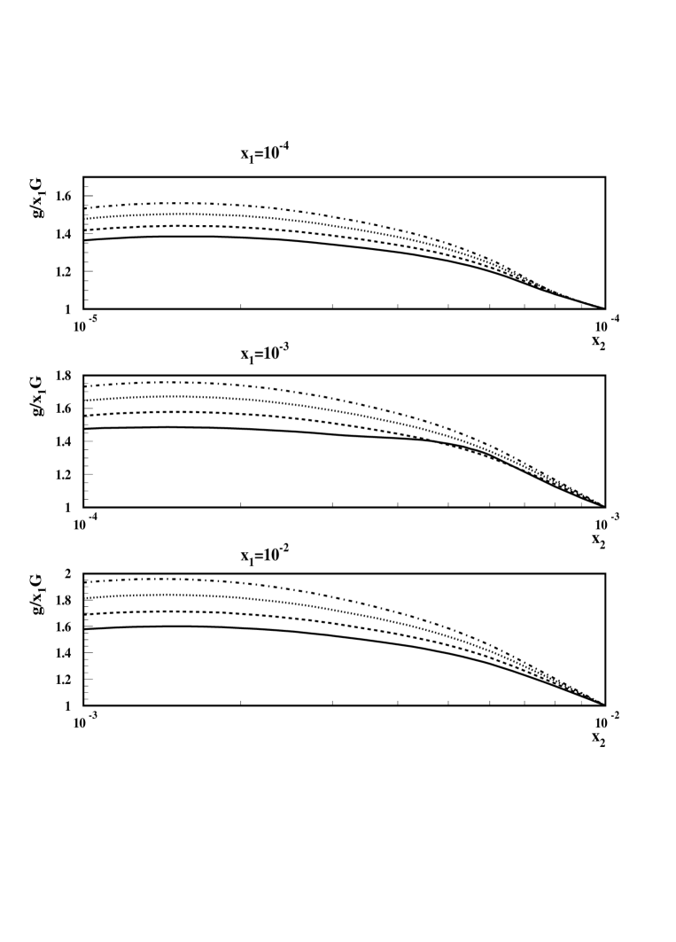
Figure 2.3: The fraction $g(x_{1},x_{2})/x_{1}G(x_{1})$ as a function of $x_{2}$ for fixed $x_{1}$ and $Q=9.3~{}\mbox{(solid line)}$, $~{}17.1~{}\mbox{(dotted line)}$, $~{}40.3~{}\mbox{(dashed line)}$ and $110~{}\mbox{(dashed-dotted line)}~{}\mbox{GeV}^{2}$.

Chapter 3 Methods in the LO Evolution of Nondiagonal Parton Distributions: The DGLAP Case

3.1 Introduction

In this chapter, which is based on Ref. [41], we give an exposition of the algorithms used to numerically solve the generalized GLAP-evolution equations of the last chapter. The main part of the evolution program was taken over from the CTEQ package for the diagonal parton distributions from inclusive reactions. At this point in time the evolution kernels for generalized parton distributions are known only to leading order in $\alpha_{s}$, as pointed out previously and thus our analysis will be a leading order one.

This chapter is organized in the following way. In Sec. 3.2 we will quickly review the formal expressions for the parton distributions and the evolution equations together with the explicit expressions for the kernels and a first comment on the resulting numerical problems. In Sec. 3.3 we will explain the difference between our algorithms and the ones used in the original CTEQ package and then give a detailed account of how we implemented our algorithms. In Sec. 3.4 we demonstrate the stability of our code and show that we reproduce the case of the usual or diagonal parton distributions within $0.5\%$ for a vanishing asymmetry factor. Sec. 3.5 contains concluding remarks.

3.2 Review of Nondiagonal Parton Distributions, Evolution Equations and Kernels

3.2.1 Nondiagonal Parton Distributions

As explained in the previous chapter, generalized or nondiagonal parton distributions occur for example in exclusive, hard diffractive $J/\psi$ or $\rho$ meson production or alternatively in deeply virtual Compton scattering (DVCS), where a real photon is produced. As mentioned in Sec. 3.1, since one imposes the condition of exclusiveness on top of the diffraction condition, one has a kinematic situation in which there is a non-zero momentum transfer onto the target proton as evidenced for example by the lowest order “handbag” diagram of DVCS in Fig. 3.1.

Figure 3.1: The lowest order handbag contribution to DVCS with $Q^{2}=-q^{2}$ and $q^{\prime 2}=0$.

The nondiagonal quark and gluon distributions have the following formal definition as matrix elements of bilocal, path-ordered and renormalized quark and gluon operators sandwiched between different momentum states of the proton as in the factorization theorems for exclusive vector meson production [25] and DVCS [43, 47, 48]:

$$f_{q/p}=\int^{\infty}_{-\infty}\frac{dy^{-}}{4\pi}e^{-ix_{2}p^{+}y^{-}}\langle p|T\bar{\psi}(0,y^{-},{\bf 0_{\perp}})\gamma^{+}{\it P}\psi(0)|p^{\prime}\rangle,$$

$$f_{g/p}=-\int^{\infty}_{-\infty}\frac{dy^{-}}{2\pi}\frac{1}{x_{1}x_{2}p^{+}}e^{-ix_{2}p^{+}y^{-}}\langle p|TG_{\nu}^{+}(0,y^{-},{\bf 0_{\perp}}){\it P}G^{\nu+}(0)|p^{\prime}\rangle.$$ (3.1)

with $x_{2}=x_{1}-\Delta$ where the asymmetry or nondiagonality parameter $\Delta$ is usually $x_{Bj}$ in, for example, DVCS or exclusive vector meson production however not in diffractive di-muon production where $\Delta=x_{Bj}+\xi_{1}$ and $\xi_{1}$ is the longitudinal momentum fraction of the produced time-like photon decaying into a $\mu^{+}\mu^{-}$-pair.

3.2.2 The GLAP-Evolution Equations for Nondiagonal Parton Distributions

Reprising on the discussion of chapter 2, the GLAP-evolution equations follow from the usual renormalization group transformation of the parton distributions and lead to the following evolution equations for the singlet(S) and non-singlet(NS) case [42, 26, 43]:

$$\frac{dq_{NS}(x_{1},\Delta,Q^{2})}{d\ln{Q^{2}}} = \int^{1}_{x_{1}}\frac{dy_{1}}{y_{1}}P^{NS}_{qq}q_{NS}(y_{1},\Delta,Q_{0}^{2}),$$

$$\frac{dg_{S}(x_{1},\Delta,Q^{2})}{d\ln{Q^{2}}} = \int^{1}_{x_{1}}\frac{dy_{1}}{y_{1}}\left[P^{S}_{gg}g_{S}(y_{1},\Delta,Q_{0}^{2})+P^{S}_{gq}q_{S}(y_{1},\Delta,Q_{0}^{2})\right],$$

$$\frac{dq_{S}(x_{1},\Delta,Q^{2})}{d\ln{Q^{2}}} = \int^{1}_{x_{1}}\frac{dy_{1}}{y_{1}}\left[P^{S}_{qq}q_{S}(y_{1},\Delta,Q_{0}^{2})+P^{S}_{qg}g_{S}(y_{1},\Delta,Q_{0}^{2})\right].$$ (3.2)

Note that $q_{S,NS}=x_{1}f_{q/p}$, $g_{S}=x_{1}x_{2}f_{g/p}$ and the kernels to leading order were given in the previous chapter together with a discussion on the the generalized $+$ regularization prescription.

3.3 Differences between the CTEQ and our Algorithms

Let us point out in the beginning that our code is to $99\%$ the original CTEQ-code (for more on this code see Ref. [49]). We only modified the subroutines NSRHSM, NSRHSP and SNRHS within the subroutine EVOLVE and added the subroutines NEWARRAY and NINTEGR. These routines are only dealing with the convolution integrals but not with, for example, the $Q^{2}$-integration or any other part of the CTEQ-code which remains unchanged. This is due to the fact that the main difference between the diagonal and nondiagonal evolution stems from the different kernels which only influence the convolution integration and nothing else.

In order to make the simple changes in the existing routines more obvious we will first deal with the new subroutines.

3.3.1 NEWARRAY and NINTEGR

Due to the increased complexity of the convolution integrals as compared to the diagonal case as pointed out in Sec. 3.2.2, we were forced to slightly change the very elegant and fast integration routines employed in the original CTEQ-code. The basic idea, very close to the one in the CTEQ-code, is the following: Within the CTEQ package, the parton distributions are given on a dynamical $x$- and $Q$-grid of variable size where the convolution of the kernels with the initial distribution is performed on the $x$-grid. Due to the possibility of singular behavior of the integrands, we perform the convolution integrals by first splitting up the region of integration according to the number of grid points in $x$, analytically integrating between two grid points $x_{i}$ and $x_{i+1}$ where $i$ runs from $1$ to the specified number of points in $x$ and then adding up the contributions from the small intervals as exemplified in the following equation:

$$\int^{1}_{x_{1}}\frac{dy_{1}}{y_{1}}Kf(x_{1}/y_{1},\Delta/y_{1},y_{1})=\Sigma_{i=0}^{N}\int^{x_{i+1}}_{x_{i}}\frac{dy_{1}}{y_{1}}Kf(x_{1}/y_{1},\Delta/y_{1},y_{1}),$$ (3.3)

where $Kf(x_{1}/y_{1},\Delta/y_{1},y_{1})$ is the product of the initial distribution for each evolution step and an evolution kernel with $x_{0}=x_{1}$, $x_{N}=1$. We can do the integration analytically between two neighboring grid points by approximating the distribution function $f(y_{1})$ through a second order polynomial $ay_{1}^{2}+by_{1}+c$, using the fact that we know the function on the grid points $x_{i-1},x_{i}$ and $x_{i+1}$ and can thus compute the coefficients a,b,c of the polynomial in the following way, given the function is well behaved and the neighboring grid points are close together :

$$f(x_{1+1}) = ax^{2}_{i+1}+bx_{i+1}+c$$

$$f(x_{i}) = ax^{2}_{i}+bx_{i}+c$$

$$f(x_{i-1}) = ax^{2}_{i-1}+bx_{i-1}+c$$ (3.4)

which yields a $3\times 3$ matrix relating the coefficients of the polynomial to the values of the distribution functions at $x_{i-1},x_{i}$ and $x_{i+1}$. Inverting this matrix in the usual way one obtains a matrix relating the $x$ values of the distribution function to the coefficients making it possible to compute them just from the knowledge of the different $x$ values and the value of the distribution function at those $x$ values. This calculation is implemented in NEWARRAY where the initial distribution is handed to the subroutine and the coefficient array is then returned. The coefficient array in which the values of the coefficients for the integration are stored, has $3$ times the size of the user-specified number of points in $x$ since we have $3$ coefficients for each bin in $x$. We treat the last integration between the points $x_{0}$ and $x_{1}$ by approximating the distribution in this last bin through a second order polynomial. However, for this last bin, the coefficients are computed using the last three values in $x$ and of the distribution at those points, since the point $x_{-1}$ which would be required according to the above prescription for calculating the coefficients, does not exist.

After having regrouped the terms appearing in the convolution integral in such a way that all the necessary cancelations of large terms occur within the analytic expression for the integral and not between different parts of the convolution integral, the integration of the different terms is performed in the new subroutine NINTEGR with the aid of the coefficient array from NEWARRAY.

As mentioned above the convolution integral from $x_{1}$ to $1$ is split up into several intervals in which the integration is carried out analytically. To give an example of this procedure we consider the convolution integral of $P_{qg}(x_{1}/y_{1},\Delta/y_{1})$ with the parton distribution $g_{S}(y_{1})$:

$$\int^{1}_{x_{1}}\frac{dy_{1}}{y_{1}}P_{qg}g_{S}=\int^{1}_{x_{1}}\frac{dy_{1}}{y_{1}}\frac{x^{2}_{1}(x_{1}-\Delta)}{y_{1}(y_{1}-\Delta)^{2}}g_{S}(y_{1})+\int^{1}_{x_{1}}\frac{dy_{1}}{y_{1}}\frac{x_{1}(y_{1}-x_{1})^{2}}{y_{1}(y_{1}-\Delta)^{2}}g_{S}(y_{1})$$ (3.5)

suppressing presently irrelevant factors in front of the integral. The two parts in Eq. (3.5) are calculated in different parts of NINTEGR and then put together in either NSRHSM, NSRHSP or SNRHS.

In NINTEGR the integrals are split up according to Eq. (3.3) and then analytically evaluated in the different $x$-bins . If the dependence of the integrand on $\Delta$ is only of a multiplicative nature it is enough to compute the integral for each bin once. To get the value of the convolution integral for a term with such a $\Delta$ dependence, it is enough to store the result of the integration in the bin from $x_{N-1}$ to $x_{N}$ in the output array for this term at the position $N-1$ , add to this result the value of the integral in the bin from $x_{N-2}$ to $x_{N-1}$ and store it at the position $N-2$ and so forth. In this manner one only has to calculate $N-1$ integrals, however if the integrand has a more complicated dependence on $\Delta$ like $x_{1}-\Delta$ one needs to compute $N(N-1)/2$ integrals. For example in order to find the integration value for the $x_{N-1}$ bin with $x_{1}=x_{N-1}$ one needs only one integral but at $x_{N-2}$ we have to redo our integral for the $x_{N-1}$ bin since $x_{1}=x_{N-2}$ plus we need to add the contribution from the $x_{N-2}$ bin to get the correct answer for the output array at position $N-2$ and so forth. This need for additional evaluations of integrals slows the program down but in the end it turns out to be only about a factor of $4-5$ slower than the original CTEQ-code which is speed optimized. The integral with the regular + - prescription is evaluated using the routine HINTEG from the original CTEQ-code whereas the generalized + - prescription is evaluated according to the methods described above due to its nontrivial dependence on $x_{1}$ and $\Delta$.

In the case of $\Delta<<x_{1}$ the analytic expressions obtained for the above general case are expanded to first order in $\Delta$ and then the same methods as above for evaluating the integrals are applied. The last case also allows us to go to the diagonal case by setting $\Delta=0$ without using the integration routines from the original CTEQ-code giving us a valuable tool to compare our code to the original one.

3.3.2 Modifications in NSRHSM, NSRHSP and SNRHS

The modification in the already existing routines NSRHSM, NSRHSP and SNRHS of the original CTEQ package are rather trivial. The most notable difference is that the subroutine NEWARRAY is called every time either of the three subroutines is called since the distribution function handed down on an array changes with every call of NSRHSM, NSRHSP and SNRHS. In NSRHSM and NSRHSP, NEWARRAY is only called once since one is only dealing with the non-singlet part containing no gluons, whereas in SNRHS the subroutine for the singlet case, one needs a coefficient array for both the quark and the gluon. Besides this change, the calls for INTEGR are replaced by NINTEGR according to how the convolution integral has been regrouped as explained in Sec. 3.3.1. The different regrouped expressions are then added, after integration for different $x$-values, to obtain the final answer in an output array which is handed back to the subroutine EVOLVE. The method is the same as in the original CTEQ-code but the terms themselves have changed of course.

3.4 Code Analysis

As a first step we tested the stability and speed of convergence of the code and found that by doubling the number of points in the $x$-grid, which is only relevant for the convolution integral, from $50$ to $300$ the result of our calculation changed by less than $0.5\%$, hence we can assume that our code converges rather rapidly. We also found the code to be stable down to an $x_{2}=10^{-10}$ beyond which we did not test. Furthermore we can reproduce the result of the original CTEQ-code, i.e. the diagonal case in LO within $0.4\%$ giving us confidence that our code works well since the analytic expressions for the diagonal case are the expansions of the general case of non-vanishing asymmetry up to, but not including, $O(\Delta^{2})$.

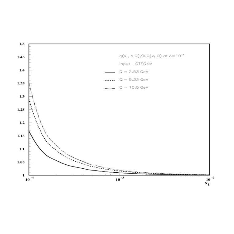
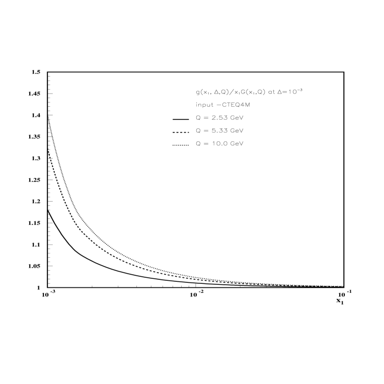
Figure 3.2: $R_{g}$ is plotted versus $x_{1}$ for fixed $\Delta$ using the CTEQ4M parameterization with $Q_{0}=$1.6 GeV and $\Lambda$ = 202 MeV.

In the following figures (Fig. 3.2-3.7) we compare, for illustrative purposes, the diagonal and nondiagonal case by plotting the ratio

$$R_{g}(x_{1},x_{2},Q^{2})=\frac{g(x_{1},x_{2},Q^{2})}{x_{1}G(x_{1},Q^{2})}$$

$$R_{q}(x_{1},x_{2},Q^{2})=\frac{q(x_{1},x_{2},Q^{2})}{x_{1}Q(x_{1},Q^{2})},$$ (3.6)

for various values of $x_{1}$, $Q^{2}$ and $\Delta=x_{Bj}$ ,i.e. , varying $x_{2}$, using the CTEQ4M and CTEQ4LQ parameterizations [40]. We assume the same initial conditions for the diagonal and nondiagonal case (see Ref. [42] for a detailed physical motivation of this ansatz).

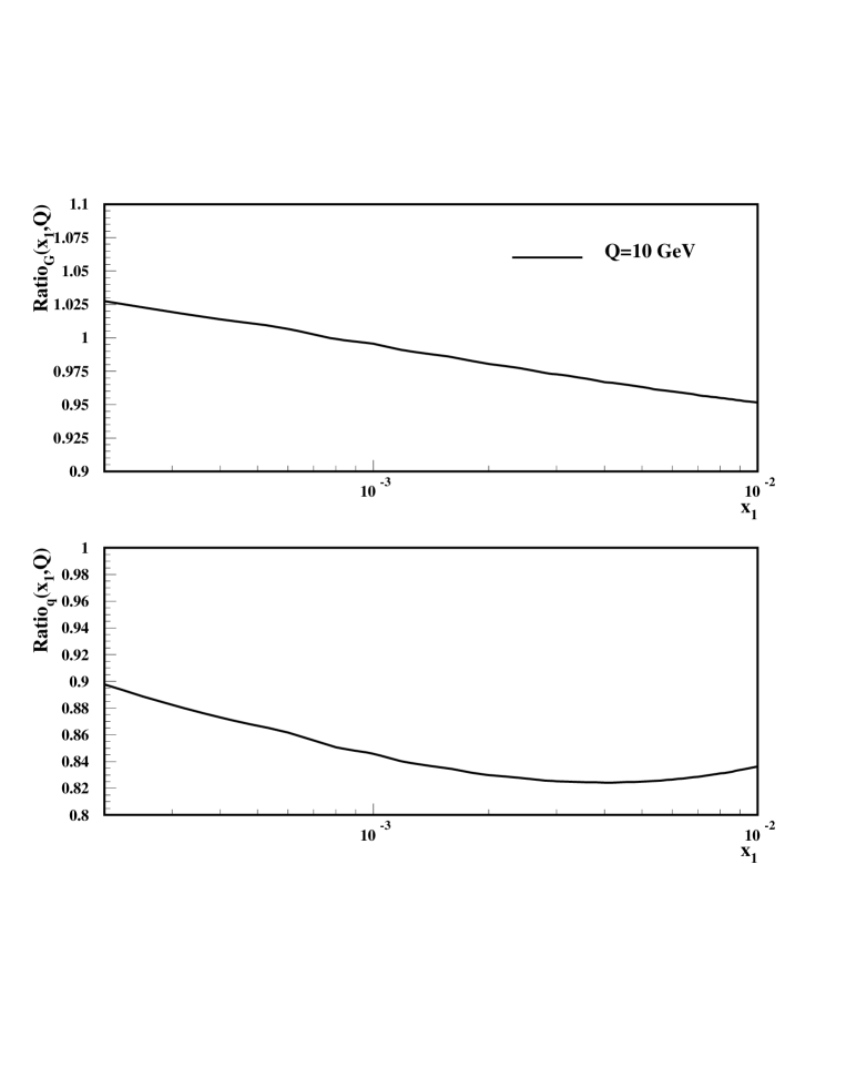
Figure 3.8: The ratios for CTEQ4M to CTEQ4LQ for gluons and quarks in the diagonal case is plotted to demonstrate the difference between the LO evolution for these parameterizations.

The reader might wonder why only CTEQ4M and CTEQ4LQ and not GRV or MRS were used. The answer is not a prejudice of we against GRV or MRS but rather the fact that a comparison of CTEQ4M and CTEQ4LQ shows the same characteristic as comparing, for example, CTEQ4M and GRV at LO. The observation is the following: CTEQ4LQ is given at a different, rather low, $Q$, as compared to CTEQ4M and hence one has significant corrections from NLO terms in the evolution at these scales. This leads to a large difference between CTEQ4LQ and CTEQ4M (see Fig. 3.8), if one evolves the CTEQ4LQ set from its very low $Q$ scale to the scale at which the CTEQ4M distribution is given, making a sensitivity study of nondiagonal parton distributions for different initial distributions impossible at LO. Of course, the inclusion of the NLO terms corrects this difference in the diagonal case but since there is no NLO calculation of the nondiagonal case available yet, a study of the sensitivity of nondiagonal evolution to different initial distributions has to wait.

The figures themselves suggest the following. First, the lower the starting scale, the stronger the effect of the difference of the nondiagonal evolution as compared to the diagonal one and also that most of the difference between nondiagonal and diagonal evolution stems from the first few steps in the evolution at lower scales.Secondly, under the assumption that the NLO evolution in the nondiagonal case will yield the same results for the parton distributions at some scale $Q$, irrespective of the starting scale $Q_{0}$, in analogy to the diagonal case. One can say that the NLO corrections to the nondiagonal evolution will be in the same direction and same order of magnitude as the diagonal NLO evolution. If, in the nondiagonal case, the NLO corrections were in the opposite direction, which would lead to a marked deviation from the LO results, compared to the diagonal case, the overall sign of the NLO nondiagonal kernels would have to change for some $\Delta\neq 0$ since in the limit $\Delta\rightarrow 0$ we have to recover the diagonal case. This occurance is not likely for the following reason: First, the Feynaman diagrams involved in the calculation of the NLO nondiagonal kernels are the same as in the diagonal case, except for the different kinematics, therefore, we have a very good idea about the type of terms appearing in the kernels, namely polynomials, logs and terms in need of regularization such as $\ln(z)\frac{\ln(1-z)}{(1-z)}$. Moreover, the kernels, as stated before, have to reduce to the diagonal case in the limit of vanishing $\Delta$ which fixes the sign of most terms in the kernel, thus the only type of terms which are allowed and could change the overall sign of the kernel are of the form

$$\frac{\Delta}{y_{1}}f(x_{1}/y_{1},\Delta/y_{1})$$ (3.7)

which will be numerically small unless $y_{1}\simeq\Delta$ in the convolution integral of the evolution equations. Moreover, we know that in this limit the contribution of the regularized terms in the kernel give the largest contributions in the convolution integral and therefore sign changing contributions in the nondiagonal case would have to originate from regularized terms. This in turn disallows a term like Eq. (3.7) due to the fact that regularized terms are not allowed to vanish in the diagonal limit, since the regularized terms arise from the same Feynman diagrams in the both diagonal and nondiagonal case. Therefore, the overall sign of the contribution of the NLO nondiagonal kernels will be the same as in the diagonal case.

A word should be said about how the results of Ref. [45] compare to ours. For the case of the same $\Delta=10^{-3}$ similar starting scales and almost identical values of $Q$ we find good agreement with their numbers for $R_{g}$ at $x_{1}\simeq\Delta$ and are slightly higher at larger $x_{1}$. The observed differences are due to the fact that the quark distributions are included in our evolution as compared to [45] and their initial distributions are slightly different. We also find very similar ratios to [45] if one changes the starting scale to a lower one. The slight difference of a few percent in the ratios between us and [45] can again be attributed to the fact that they used the GRV distribution as compared to our use of the CTEQ4 distributions, hence a slight difference in the starting scales and their lack of incorporating quarks into the evolution.

3.5 Conclusions

We modified the original CTEQ-code in such a way that we can now compute the evolution of nondiagonal parton distributions to LO. We gave a detailed account of the modifications and the methods employed in the new or modified subroutines. As the reader can see, the modifications and methods themselves are not something magical but rather a straightforward application of well known numerical methods. We further demonstrated the rapid convergence and stability of our code. In the limit of vanishing asymmetry we reproduce the diagonal case in LO as obtained from the original CTEQ-code within $0.4\%$. We also have good agreement with the results in Ref. [45]. In the future, after the NLO kernels for the nondiagonal case have been calculated, we will extend the code to the NLO level to be on par with the diagonal case.

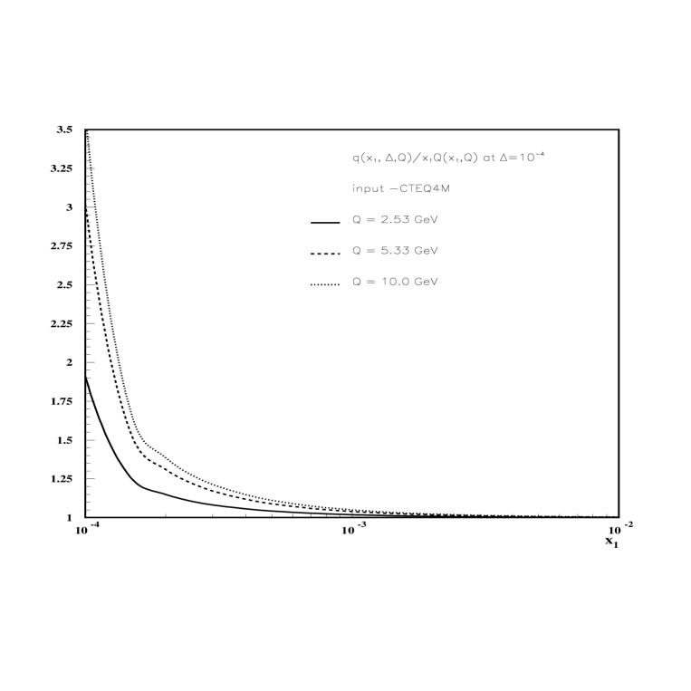
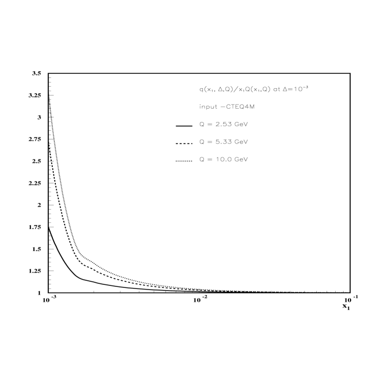
Figure 3.3: $R_{q}$ is plotted versus $x_{1}$ for fixed $\Delta$ using the CTEQ4M parameterization with $Q_{0}=$1.6 GeV and $\Lambda$ =202 MeV.

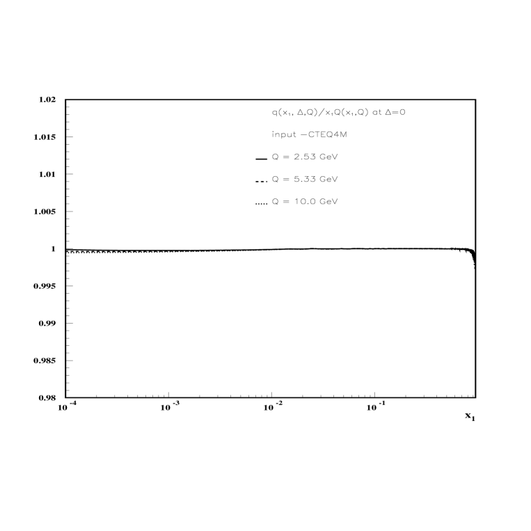
Figure 3.4: $R_{g}$ and $R_{q}$ are plotted versus $x_{1}$ for $\Delta=0$ using the CTEQ4M parameterization with $Q_{0}=$1.6 GeV and $\Lambda$ = 202 MeV.

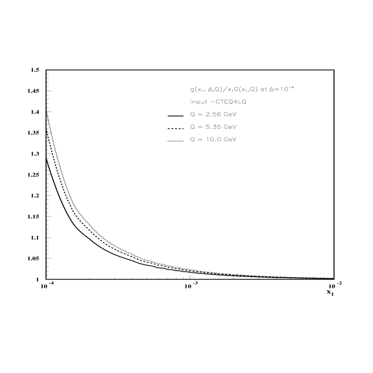
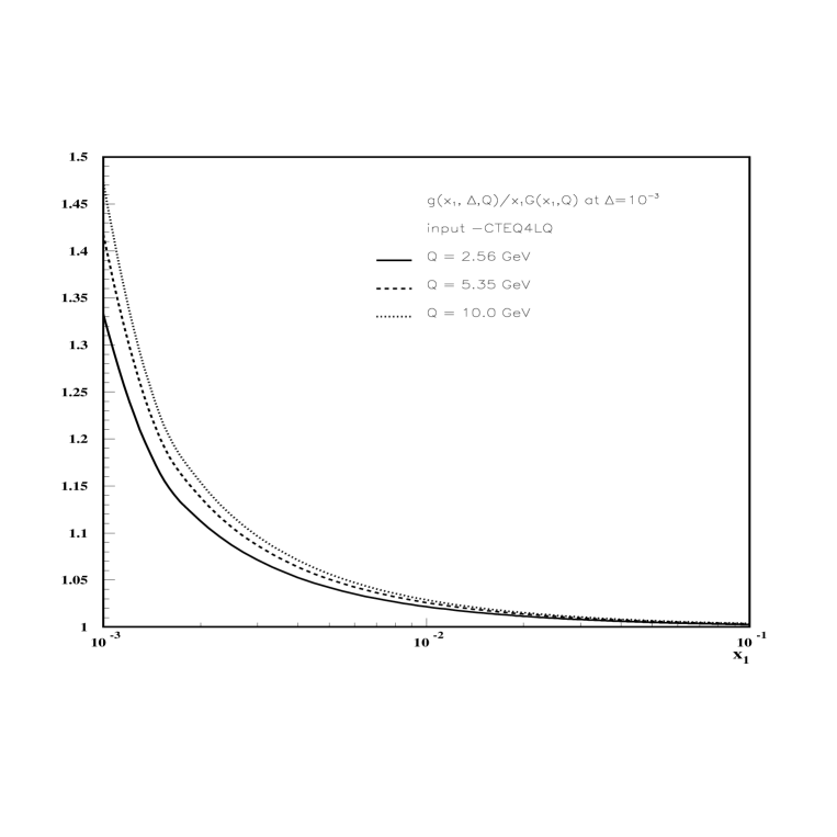
Figure 3.5: $R_{g}$ is plotted versus $x_{1}$ for fixed $\Delta$ using the CTEQ4LQ parameterization with $Q_{0}=$0.7 GeV and $\Lambda$ =174 MeV.

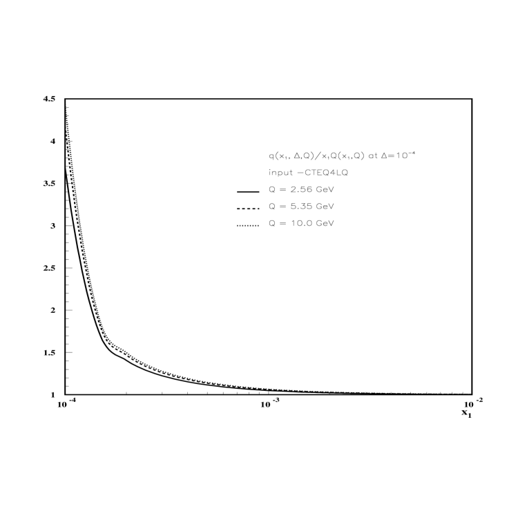
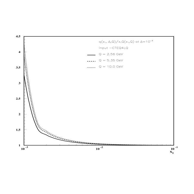
Figure 3.6: $R_{q}$ is plotted versus $x_{1}$ for fixed $\Delta$ using the CTEQ4LQ parameterization with $Q_{0}=$0.7 GeV and $\Lambda$ =174 MeV.

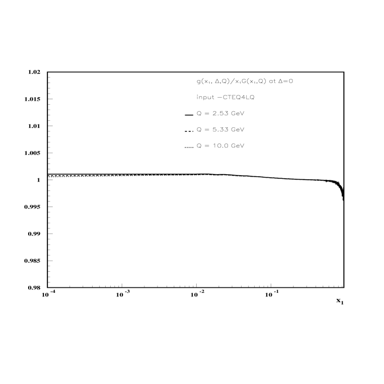
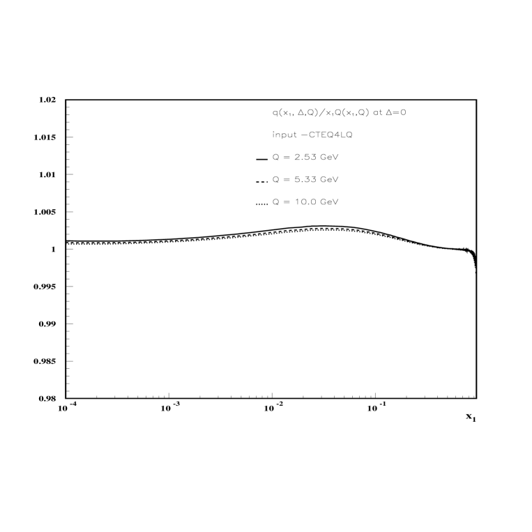
Figure 3.7: $R_{g}$ and $R_{q}$ are plotted versus $x_{1}$ for $\Delta=0$ using the CTEQ4LQ parameterization with $Q_{0}=$0.7 GeV and $\Lambda$ =174 MeV.

Chapter 4 Proof of Factorization for Deeply Virtual Compton Scattering in QCD

4.1 Introduction

In this chapter, based on Ref. [47], we prove factorization for the deeply virtual Compton scattering (DVCS) amplitude in QCD up to power suppressed terms, to all orders in perturbation theory. This proof is important because of the recent great interest in DVCS [26, 50, 51, 52, 53, 54, 55, 56, 57]. One important use of DVCS is as a probe of off-forward (or nondiagonal) distributions [26, 50, 58, 25, 42]. These differ from the usual parton distributions probed in inclusive reactions by having a non-zero momentum transfer between the proton in the initial and final state.

A related process which is also used to probe off-diagonal parton densities is exclusive meson production in deep-inelastic scattering [22, 59], for which a proof of factorization was given in [25]. Compared with this process, DVCS is simpler because the composite meson in the final state is replaced by an elementary particle, the photon, and thus there is no meson wave function in the factorization formula.

Ji [26] and Radyushkin [50] have provided the key insights that indicate that a factorization theorem is valid for DVCS and Radyushkin also gave an all-orders proof [50]. In this chapter, we provide an alternative proof, and give a new treatment of some problems that were touched upon in Ref. [50] but that were not fully solved. The proof follows the general lines of proofs of factorization for other processes [35, 36], and the most noteworthy feature is that the proof is simpler than for any other process. Even for ordinary deep-inelastic scattering one needs to discuss the cancelation of soft gluon exchanges and of final-state interactions, whereas these complications are not present in the leading power for DVCS.

The chapter is organized in the following way: First we will state the theorem to be proved in Sec. 4.2 and then explain the steps necessary to prove it, as adapted from Ref. [25], in Sec. 4.3. The complications mentioned above concern the situation when one of the two lines connecting the parton density to the hard scattering carries zero longitudinal momentum, and these are given a detailed treatment in Sec. 4.3.8. In the last section we will make concluding remarks.

4.2 Factorization Theorem

The process under consideration is DVCS, which is the elastic scattering of virtual photons:

$$\gamma^{*}(q)+P(p)\rightarrow\gamma^{(*)}(q^{\prime})+P^{\prime}(p-\Delta)$$ (4.1)

where the diffracted proton $P^{\prime}$ may also be replaced by a low-mass excited state and the final-state photon can be either real or time-like. This process is the hadronic part of $ep\rightarrow e\gamma p^{\prime}$ for a real photon or of $ep\rightarrow e\mu^{+}\mu^{-}p^{\prime}$ for a time-like photon.

It is convenient to use light-cone coordinates with respect to the collision axis. The momenta in the process then take the form:

$$p^{\mu} = \left(p^{+},\frac{m^{2}}{2p^{+}},{\bf 0}_{\perp}\right),$$

$$q^{\mu} \simeq \left(-xp^{+},\frac{Q^{2}}{2xp^{+}},{\bf 0}_{\perp}\right),$$

$$q^{\prime\mu} \simeq \left(xp^{+}\frac{\Delta^{2}_{\perp}+\alpha Q^{2}}{Q^{2}},\frac{Q^{2}}{2xp^{+}},{\bf\Delta}_{\perp}\right),$$

$$\Delta^{\mu} \simeq \left(x(1+\alpha)p^{+},-\frac{\Delta^{2}_{\perp}+m^{2}(1+\alpha)x}{2(1-x-\alpha x)p^{+}},{\bf\Delta}_{\perp}\right).$$ (4.2)

Here, $x$ is the Bjorken scaling variable, $Q^{2}$ is the virtuality of the initial photon, $m^{2}$ is the proton mass, $t=\Delta^{2}$ is the momentum transfer squared, and $\alpha$ is a parameter that specifies the virtuality of the outgoing photon: ${q^{\prime}}^{2}=\alpha Q^{2}$. Thus, $\alpha=0$ for a real photon and $\alpha>0$ for a time-like photon. Finally, $\simeq$ means “equality up to power suppressed terms”.

The theorem to be proved is that the amplitude for the process (4.1) is:

$$T=\Sigma_{i}\int_{-1+x}^{1}dx_{1}f_{i/p}\left(x_{1},x_{2},t,\mu\right)H_{i}\left(x_{1}/x,x_{2}/x,\mu\right)\,+\,\mbox{power-suppressed corrections},$$ (4.3)

where the $f_{i/p}$ is a nondiagonal parton distribution and $H_{i}$ is the hard-scattering coefficient for scattering off a parton of type $i$. We let $x_{1}$ be the momentum fraction of parton $i$ coming from the proton, so that $x_{2}=x_{1}-(1+\alpha)x$ is the momentum fraction which is returned to the proton by the other parton line joining the parton distribution and the hard scattering. There is implicit polarization dependence in the amplitude. $\mu$ is the usual renormalization/factorization scale which should be of order $Q$ to allow calculations of the hard scattering coefficients within finite-order perturbation theory. The $\mu$ dependence of $f_{i/p}$ is given by equations of the DGLAP and Brodsky-Lepage kind [26, 50, 58, 22, 25, 42]. The parton distributions in Eq. (4.3), together with their evolution equations, are defined using the conventions of [25, 42]. They may easily be transformed into those given in [26, 50] by a change of normalization and of kinematic variables.

4.3 Proof of Theorem

The proof of our theorem Eq. (4.3) can be summarized as follows :

• Establish the non-ultra-violet regions in the space of loop momenta contributing to the amplitude.

• Establish and prove a power counting formula for these regions.

• Determine the leading regions of the amplitude.

• Define the necessary subtractions in the amplitude to avoid double counting.

• Taylor expand the amplitude to obtain a factorized form.

• Show that the part containing the long-distance information can be expressed through matrix elements of renormalized, bi-local, gauge invariant operators of twist-$2$.

4.3.1 Regions

First let us establish the regions in the space of loop momenta contributing to the asymptotics of the amplitude, i.e., the generalized reduced graphs. The steps leading to the generalized reduced graphs are identical to the steps 1–3 in Sec. IV of Ref. [25], i.e., scale all momenta by a factor $Q/m$, use the Coleman-Norton theorem to locate all pinch-singular surfaces in the space of loop momenta (in the zero-mass limit), and finally identify the relevant regions of integration as neighborhoods of these pinch-singular surfaces.

In the first step, the scaling of momenta, we proceed as follows [60]. We write the general momentum $k^{\mu}$ and a general mass $m$ in units of the large scale $Q$:

$$k^{\mu}=Q\tilde{k}^{\mu},~{}~{}~{}~{}~{}~{}m=Q\tilde{m}.$$ (4.4)

Due to working in the rest frame of the virtual photon both of the light like components are of order $Q$. Therefore, when everything is expressed in terms of the above scaled variables, dimensional analysis shows that the large $Q$ limit is equivalent to the $\tilde{m}\rightarrow 0$ limit. Since the amplitude is dimensionless we have

$$T(Q^{2},p,q^{\prime},\Delta,m;\mu)=T(1,\tilde{p},\tilde{q}^{\prime},\tilde{\Delta},\tilde{m},Q/\mu),$$ (4.5)

by regular dimensional analysis.

The most basic region is found where all internal lines obey $k^{2}\geq Q^{2}$, with the scaled momenta $\tilde{k}$ having virtualities of $1$ or bigger. In such a region one is entitled to setting the masses equal to zero, make the external hadrons light-like and set the renormalization scale $\mu$ equal to $Q$, thus avoiding large logarithms. As it turns out, however, this region is not only not the only one but it is even not leading. Nevertheless, one can now see that all other relevant regions correspond to singularities of massless Feynman graphs. They are neighborhoods of pinch-singular surfaces of massless graphs, in other words, surfaces where the loop momenta are trapped at singularities. The conditions for a pinch singularity are the Landau conditions for a singularity of a graph. Only pinch singularities are of interest, since at a non-pinched singularity, one can deform the contour of integration such that at least one of the singular propagators is no longer near its pole. In case of a pinch singularity from propagator poles in the massless limit, we know then that in the real graph, with nonzero masses but large $Q$, the contour of integration is forced to pass near the propagator poles. Consequently, it is not possible to neglect the masses in this region. Conversely, if the contour is not trapped by the poles, the contour can be deformed away from the poles, and the mass may be neglected in evaluating the corresponding propagators.

In the second step we use the Coleman-Norton theorem [61] which states that each point on a pinch-singular surface in loop momentum space, corresponds to a space-time diagram obtained in the following way. First one obtains a reduced graph by contracting to points all of the lines whose denominators are not pinched. Then one assigns space-time points to each vertex of the reduced graph in such a way that the pinched lines correspond to classical particles. In other words each line is assigned a particle propagating between space-time points corresponding to the vertices at its ends. The momentum of the particle is exactly the momentum carried by the line, with its orientation such that it has positive energy. If, for some set of momenta, one cannot construct such a reduced graph, one is free to deform the contour of integration. A reduced diagram, therefore, corresponds to a classically allowed space-time scattering process. In the zero mass limit, the construction of reduced graphs becomes very simple, since all pinched lines must carry either light-like or zero momentum. Furthermore, each light-like momentum must be parallel to one of the, now light-like, external lines.

To be precise, in the zero mass limit of the process under consideration we have:

• One light-like incoming proton of momentum $p^{\mu}_{A}=(p^{+},0,0_{\perp})$.

• One light-like outgoing proton line of parallel momentum
  $p^{\prime\mu}_{A}=((1-(1+\alpha)x)p^{+},0,0_{\perp})$.

• One light-like outgoing photon line of momentum $q^{\prime\mu}=(\alpha xp^{+},Q^{2}/2xp^{+},0_{\perp})$.

• One incoming virtual photon of momentum $q^{\mu}=(-xp^{+},Q^{2}/2xp^{+},0_{\perp})$.

Figure 4.1: a) Reduced graph for DVCS with direct coupling for the out-going photon to hard subgraph. b) The same without a direct coupling for the out-going photon.

The results of the above construction are the two kinds of reduced graph shown in Fig. 4.1. There, $A$ and $B$ denote collinear graphs with one large momentum component in the $+$ and $-$ direction respectively, $H$ denotes the hard scattering graph, and $S$ denotes a graph with all of its lines soft, i.e., in the center-of-mass frame all the components of the momenta in $S$ are much smaller than $Q$. Note that, of the external momenta, $p$ and $p^{\prime}$ belong to $A$, $q^{\prime}$ belongs to $B$ or $H$ , and $q$ belongs to $H$.

When the two external photons have comparably large virtualities, the only reduced graphs are of the first kind, Fig. 4.1a, where the out-going photon couples directly to the hard scattering. But when the outgoing photon has much lower virtuality than the incoming photon, for example, when it is real, we can also have the second kind of reduced graph, Fig. 4.1b, where the out-going photon couples to a $B$ subgraph. As we will see later, power counting will show that the second kind of reduced graph, Fig. 4.1b, is power suppressed compared to the first kind, with a direct photon coupling. This implies that we will avoid all the complications which were encountered in [25] that are associated with the meson wave function.

Figure 4.2: a) Space-time picture of the DVCS process with a collinear-to-$B$ part as in vector meson production. b) Space-time picture of the DVCS process without a collinear-to-$B$ part.

The corresponding space-time diagram is Fig. 4.2. In this figure, each solid line corresponds to a light-like line of the reduced graphs, with a $45^{\circ}$ orientation to correspond to their light-like lines of propagation. The dashed lines correspond to the soft subgraph $S$. As far as the Coleman-Norton theorem is concerned the lines are degenerate. In fact they are carrying zero-momentum implying that they have no specific orientation. They are therefore indicated by curved lines of no particular orientation. The location of the endpoints of the soft lines can be anywhere along the world lines of the collinear lines. The hard vertex $H$ occurs at the intersection of the collinear lines. The world line , in the $+$ direction, of the collinear-to-$A$ subgraph actually consists of several lines propagating together and possibly interacting with each other.

In the space-time representation of a Feynman graph, there is normally an exponential suppression when there are large space-time separations between vertices. One obtains a singularity when this suppression fails and the Coleman-Norton construction gives exactly the relevant configurations of the vertices. The singularity is generated by the possibility of integrating over arbitrarily large scalings in coordinate space without obtaining exponential suppressions.

Note that the above discussion relies on the use of a covariant gauge. The use of an axial gauge, albeit convenient, leads to unphysical singularities in the propagators. These singularities do not give the normal rules of causal relativistic propagation of particles and, furthermore, make the derivation of the factorization theorem, beyond leading log, very difficult [36, 37].

4.3.2 Power Counting

Each reduced graph codes a region of loop-momentum space, a neighborhood of the surface $\pi$ of a pinch singularity in the zero-mass limit. The contribution to the amplitude from a neighborhood of $\pi$ behaves like $Q^{p(\pi)}$, modulo logarithms, in the large-$Q$ limit, with the power given by

$$p(\pi) = 4-n(H)-\mbox{\#(quarks from $S$ to $A$, $B$)}-3\mbox{\#(quarks from $S$ to $H$)}$$ (4.6)

$$-2\mbox{\#(gluons from $S$ to $H$)}.$$

where $n(H)$ is the number of collinear quarks, transversely polarized gluons, and external photons attaching to the hard subgraph $H$. Such results were obtained by Libby and Sterman [60, 62]. The particular form of Eq. (4.6) was given in [25] together with a proof that applies without change to DVCS.

We will detail it here, nevertheless, for completeness sake. The arguments used in the proof will rely on general arguments about dimensional analysis and Lorentz boosts.

We first consider the case of only the hard and collinear subgraphs without a soft subgraph. Let the hard subgraph have $N_{q}$ external quark/antiquark lines and $N_{g}$ external gluons, as well as two photon lines. By definition, all components in the hard subgraph have virtuality of order $Q^{2}$. Since the hard subgraph has dimensions $d_{H}=2-\frac{3}{2}N_{q}-N_{g}$ and all the couplings are dimensionless, it contributes a power

$$Q^{d_{H}}=Q^{2-\frac{3}{2}N_{q}-N_{g}}$$ (4.7)

to the amplitude.

For the momenta collinear to the proton we have

$$\mbox{typical A momentum}\propto\left(Q,\frac{m^{2}}{Q},m\right).$$ (4.8)

Since $x$ is small, there are also collinear momenta with $+$ components much larger then $Q$. We will deal with this problem later on; let us just assume for the moment that $x$ is not small.

The collinear configurations can be obtained by boosts from a frame in which all components of all momenta are of order $m$. Since the virtualities and the sizes of regions of momentum integration are invariant under boosts, we start by assigning the collinear subgraphs an order of magnitude $m^{\mbox{dimension}}$, which contributes unity to the power of $Q$. Note that we define the collinear factors to include the integrals over the momenta of the loops that connect the collinear subgraphs and the hard subgraph.

In the next step, we have to take into account that the collinear subgraphs are coupled to the hard subgraph by Dirac and Lorentz indices. The effect of boosting a Dirac spinor from rest to the energy $Q$ is to make its largest component of order $(Q/m)^{1/2}$ bigger than the rest frame value and the effect on a Lorentz vector is to give a factor of $(Q/m)^{1}$. The exponents are just the spins of the corresponding fields. Multiplying by these powers gives

$$Q^{2-N_{q}}.$$ (4.9)

This agrees with Eq. (4.6) in the case that all external lines of the hard graph are quarks but is a factor $Q^{N_{g}}$ larger if the external particles are gluons.

The well-known problem of gluons with scalar polarization (see, for example, [35, 63]) will be dealt with later on. Suffice it to say here that gluons with such a polarization can be factorized into the parton distributions by using gauge-invariance arguments.

For the moment we just need to define the concepts of scalar and transverse polarization in the sense that we will use and show how this affects the power counting.

Consider the attachment of one gluon, of momentum $k^{\mu}$, from the collinear-to-$A$ subgraph to the hard subgraph. One has a factor $A^{\mu}g_{\mu\nu}H^{\nu}$, where $A^{\mu}$ and $H^{\nu}$ denote the collinear-to-$A$ and hard subgraph respectively, and $g_{\mu\nu}$ is the numerator of the gluon propagator in the Feynman gauge. On can now decompose this factor into components:

$$A\times H=A^{+}H^{-}+A^{-}H^{+}-A_{\perp}\times H_{\perp}.$$ (4.10)

One observes now that after the boost from the proton rest frame, the largest component of $A^{\mu}$ is the $+$ component. The largest term is therefore $A^{+}H^{-}$ and this is the term which gives the power in Eq. (4.9). The other two terms are suppressed by one or two powers of $Q$.

One can define now the following decomposition:

$$A^{\mu}=k^{\mu}\frac{A^{+}}{k^{+}}+\left(A^{\mu}-k^{\mu}\frac{A^{+}}{k^{+}}\right).$$ (4.11)

The first term will be called the scalar component of the gluon and gives a polarization vector proportional to the momentum of the gluon. The second term gives the transverse part of the gluon with no $+$ component, it, therefore, gives a contribution to $A\times H$ which is one power of $Q$ smaller than the contribution of the scalar component. The $k^{\mu}$ factor in the scalar term multiplies the hard subgraph and gives a quantity that can be simplified by the use of Ward identities.

The above decomposition will now be applied to every gluon joining the subgraphs $A$ and $H$. The contribution of our region to the amplitude is now a sum of terms in which each of these gluons is either scalar or transverse. Each term has a power

$$Q^{2-N_{q}-N_{g}}Q^{N_{s}}=Q^{2-N_{q}-N_{T}};$$ (4.12)

where $N_{s}$ is the number of scalar gluons and $N_{T}=N_{g}-N_{s}$ is the number of transverse gluons that enter the hard scattering. This is exactly the power in Eq. (4.6) without a soft subgraph.

In Taylor expanding the hard subgraph, we will need to slightly modify the above decomposition in Eq. (4.11) and also apply an exactly analogous argument to the couplings of soft gluons to a collinear graph.

One will also need to pick out the largest component of the Dirac structure of the collinear subgraphs, here however, this is not necessary to be made explicit since we do not have a cancelation of the highest power. Note that the projection of the largest Dirac component is directly reflected in the $\gamma^{+}$ factor in the definition of the quark distribution.

In the derivation of Eq. (4.12) we assumed $x$ not to be small. In the case of large $x$ then, we have to boost parts of the collinear-to-$A$ subgraph to get + momenta of order $p^{+}$ instead of $xp^{+}$. This leads to groups of lines with very different rapidities. In Feynman graphs, the effect is just to give a factor $1/x$ times logarithms, however only if the exchanged lines between the regions of different rapidities are gluons [64]. In the case of exchanged quarks, there will be a suppression factor of $x$. All of this does not influence the power of $Q$.

If one now adds in a soft subgraph $S$, one has the problem of choosing the appropriate scaling of the momenta. There are several possibilities and the literature is not entirely clear about the best scaling. In our case we will choose to have all soft momentum components of $O(m^{2}/Q)$. This has the advantage of not sending any collinear-to-$A$ lines far off-shell, the trade off is that we introduce regions where the momenta are unphysically soft in a confining theory and the power counting is mass sensitive.

With this scaling the basic power in the Breit frame is $m^{2}/Q$ to a power which is the dimension of the soft subgraph, including the integration over the soft loop momenta that circulate between S and the rest of the graph with the assumption of negligible masses. The power is simply

$$-N_{gS}-\frac{3}{2}N_{qs}$$ (4.13)

where $N_{gS}$ and $N_{qS}$ are the number of external gluons and quarks of the soft subgraph. These external lines go either into the hard subgraph in which case the dimension of the hard subgraph is reduced by $3/2$ for each extra quark and $1$ for each extra gluon or into the collinear-to-$A$ subgraph which does not affect the power of $Q$. Now we have to take into account that we are dealing with vectors and spinors connecting $S$ to $A$, this means that we have to use the same factors as before meaning we gain a factor $Q^{1/2}$ for each quark and $Q^{1}$ for each gluon.

Putting all the factors together we get for the soft to hard contribution $-N_{g}-\frac{3}{2}N_{q}-N_{g}-\frac{3}{2}N_{q}=-2N_{g}-3N_{q}$ and for the soft to collinear contribution $-N_{g}-\frac{3}{2}N_{q}+N_{g}+\frac{1}{2}N_{q}=-N_{q}$. This together with our earlier result (Eq. (4.12)) yields Eq. (4.6) .

Figure 4.3: Those reduced graphs that contribute to the leading regions in DVCS.

4.3.3 Leading Regions

The leading regions for the amplitude are those with the largest exponent $p(\pi)$ in Eq. (4.6). It is easy to see that these correspond to the reduced graphs in Fig. 4.3, independently of whether the out-going photon is real or far off-shell. The corresponding power is $Q^{0}$. These reduced graphs have direct photon couplings to the hard subgraph, they have exactly two parton lines connecting the collinear subgraph $A$ to the hard subgraph $H$, and they have no soft lines connecting to $H$. The two kinds of graph differ only by the absence or presence of a soft subgraph that connects to $A$ alone.

Among the other reduced graphs, which are non-leading for our process, are those of the type in Fig. 4.1b, which are leading in the case of diffractive meson production, where the leading region gives $Q^{-1}$.

In the case of a photon that is off-shell by order $Q^{2}$, the amplitude for production of the photon behaves like $Q^{0}$, the same as for a real photon. However, the physically observed process includes the decay of the time-like photon (to a $\mu^{+}\mu^{-}$ pair, for example), which results in a power suppression of the observed cross section by $1/Q^{2}$ compared with the cross section for making real photons.

4.3.4 Proof of absence of a soft part in leading regions

As mentioned in Sec. 4.3.3, there might, in principle, be a soft part $S$ in the leading reduced graph connected solely to the $A$ graph by gluons, as shown in Fig. 4.3b. Note that by Eq. (4.6), quarks connecting $S$ to $A$ would lead to a power suppression. We will now show that this soft part $S$ is indeed absent, and so we only need to consider regions of the form of Fig. 4.3a.

Figure 4.4: Soft gluon loop attaching to collinear line.

We will first examine a simple one loop example, Fig. 4.4. The external quark is part of the $A$ subgraph in Fig. 4.3b, and the gluon is soft. So we parameterize the momenta by:

$$k_{A} = (x_{1}p^{+},k_{A}^{-},{\bf k_{A,\perp}}),$$

$$k = (k^{+},k^{-},{\bf k_{\perp}}).$$ (4.14)

where the $k^{+}_{A}$ is $O(Q)$ and all the other components are of $O(m)$ or smaller.

If we omit irrelevant factors in the numerator, the loop integral takes the following form:

$$\int_{{\rm soft}~{}k}\frac{d^{4}k}{(k^{2}+i\epsilon)\left[(k_{A}-k)^{2}-m^{2}+i\epsilon\right]}$$

$$=\int_{{\rm soft}~{}k}\frac{d^{4}k}{(2k^{+}k^{-}-k_{\perp}^{2}+i\epsilon)\left[2(x_{1}p^{+}-k^{+})(k_{A}^{-}-k^{-})-(k_{A,\perp}-k_{\perp})^{2}-m^{2}+i\epsilon\right]}$$

$$\simeq\int_{{\rm soft}~{}k}\frac{dk_{+}}{(2k^{+}k^{-}-k_{\perp}^{2}+i\epsilon)\left[2x_{1}p^{+}(k_{A}^{-}-k^{-})-(k_{A,\perp}-k_{\perp})^{2}-m^{2}+i\epsilon\right]}.$$ (4.15)

As before, $\simeq$ stands for “equality up to power suppressed terms”. As one can see, there is no $k^{+}$-pole in the second part of the denominator and we can freely deform the contour in $k^{+}$ to avoid the pole in the soft gluon propagator. This takes us out of the soft region for $k$.

In the general situation, Fig. 4.3b, we can use a version of the arguments in Ref. [25, 66] to show that the soft momenta ${k^{+}_{i}}$ can be rerouted in such a way as to exhibit a lack of a pinch singularity. The essential idea is that one can find a path backwards or forward from one external line of $S$ to another external line of $S$. The loop is completed along lines of $A$, all of which have much larger $+$ momenta than what is typical of soft momenta, and hence there is no pinch.

4.3.5 Subtractions

The subtractions necessary to avoid double counting in the amplitude are exactly similar to the ones in Sec. VI of Ref. [25], since the distributional arguments to construct the subtraction terms on a pinch-singular surface $\pi$ presented there are very general in nature and are not limited to the case of diffractive vector meson production that was considered in [25].

Let us review the construction. For each graph $\Gamma$, there may be several different pinch singular surfaces $\pi$ in the space of loop-momentum contributing to the leading power. We write therefore the graph as a sum of those contributions

$$\mbox{Asy}\Gamma=\Sigma_{\pi}\Gamma_{\pi},$$ (4.16)

where ’Asy’ denotes the asymptotic behavior of the graph.

The term $\Gamma_{\pi}$ is obtained by Taylor expanding the hard and collinear subgraphs in powers of the small variables denoted by $T_{\pi}$. Since one can possibly have several regions contributing to a given graph, one must make subtractions to avoid double counting. This operation will be denoted by $R$. Therefore, we can write

$$\mbox{Asy}\Gamma=\Sigma_{\pi}RT_{\pi}\Gamma_{\pi}.$$ (4.17)

This is exactly analogous to the Bogoliubov $R$-operation for renormalization. The easiest way to formulate the above procedure is due to Tkachov et al. [65]. In this method the integrand of each graph $\Gamma$ is viewed as a distribution, in other words

$$\Gamma\otimes f=\int dk\Gamma(k,p)f(k),$$ (4.18)

where k denotes the collection of loop momenta, p the external momenta and $f(k)$ is a test function. Putting the test function to $1$ will give the contribution of $\Gamma$ to the amplitude.

The advantages of the methods employed in Ref. [65] are the control they give in treating different regions of momentum space separately without having sharp boundaries between different regions. Note that this is particularly convenient in our case where one has to deform contours of integration away from pinch singularities. If we were to use sharp boundaries these deformations would be impossible.

Using this language, the contribution $\Gamma_{\pi}$ to Asy$\Gamma$ from the neighborhood of a pinch-singular surface $\pi$ is localized on the surface, in other words is proportional to a $\delta$-function that restricts the integration to the surface. One then defines a hierarchy of regions through set-theoretic inclusion: $\pi_{1}>\pi_{2}$ means that the pinch-singular surface $\pi_{1}$ contains $\pi_{2}$. One than constructs any $\pi$ on the assumption that the terms for all bigger regions have already been constructed. Thus one has a recursive construction starting from the largest region.

Assume that one has constructed the terms $\Gamma_{\pi^{\prime}}$ for all regions bigger than $\pi$ and then decompose Asy$\Gamma$ as

$$\mbox{Asy}\Gamma=\Sigma_{\pi^{\prime}>\pi}\Gamma_{\pi^{\prime}}+\Gamma_{\pi}+~{}\mbox{other terms}.$$ (4.19)

The “other terms” correspond to three classes of surfaces. The first class are those surfaces that are smaller than $\pi$, the second class consists of those that intersect $\pi$ in a subset of $\pi$, i.e. , they have a lower dimension and the third class are those that do not intersect $\pi$ at all.

The hypothesis for our induction is that the sum of $\Gamma_{\pi^{\prime}}$ over $\pi^{\prime}>\pi$ gives a good approximation to the original $\Gamma$ except in the neighborhoods of the smaller surfaces for which $\Gamma_{\pi}$ has not yet been constructed. The integrals defining the $\Gamma_{\pi}$’s cover the whole space of integration variables, but are only required to give a good approximation if one excludes neighborhoods of smaller surfaces. This means that we require the test function in Eq. (4.18) to be zero on these smaller surfaces. When $\Gamma_{\pi}$ is combined with the $\Gamma_{\pi^{\prime}}$ for larger surfaces it must give a good approximation to $\Gamma$ on a neighborhood of $\pi$. Note that a good approximation is not necessary on the surfaces where the test function is zero; there is no need for $\Gamma_{\pi^{\prime}}$ to be constructed for the smaller surfaces since they will give zero with such a test function. This is enough to prove the inductive hypothesis for the next recursive step.

Since $\Gamma_{\pi}$ is located on $\pi$, it is necessary to consider only a neighborhood of $\pi$. This combined with the statement in the previous paragraph ensures that there is no need for the unconstructed “other terms” in order to construct $\Gamma_{\pi}$.

One can therefore define

$$\Gamma_{\pi}=T_{\pi}\left[\Gamma-\Sigma_{\pi^{\prime}>pi}R\Gamma_{\pi^{\prime}}\right],$$ (4.20)

where $T_{\pi}$ stands for a Taylor expansion in powers of the small variables on $\pi$. The first term is the Taylor expansion of the original graph and the remaining terms can be thought of as subtractions that prevent double counting of contributions to the integral over a neighborhood of $\pi$.

This results in a sum over $\Gamma_{\pi}$ and the terms for the larger regions

$$\Gamma_{\pi}+\Sigma_{\pi^{\prime}>\pi}R\Gamma_{\pi^{\prime}},$$ (4.21)

giving the correct contribution to the asymptotics of $\Gamma$ that originates from a neighborhood of $\pi$ and of all larger regions. Neighborhoods of smaller regions are, of course, excluded.

In general $\Gamma_{\pi}$ gives a divergence when integrated with a test function over a neighborhood of any of these smaller regions. Therefore, it is only defined when integrated with a test function which is $0$ on these smaller regions. We now extend this distribution to a distribution defined on all test functions by adding infra-red counterterms to cancel the arising divergences from the smaller regions. This operation is analogous to the well known $+$ distribution employed earlier in this thesis. The result will be $R\Gamma_{\pi}$ with the counterterms all being local in momentum space. Choosing a definition of $\Gamma_{\pi}$ on the smaller surfaces is perfectly satisfactory, since we have not yet considered how to approximate $\Gamma$ in regions smaller than $\pi$. We only require $R\Gamma_{\pi}$ to be finite and the counterterms to be localized on smaller surfaces than $\pi$ in order not to affect the good approximation we have for $\pi$ and larger surfaces. Continuing with the recursion, one eventually obtains appropriate approximations for these smaller surfaces.

Note that the subtraction terms, as defined in Eq. (4.20), ensure that changes in the choice of counterterms localized on any particular surface $\pi$ are cancelled by corresponding changes in the subtraction terms in the definition of $\Gamma_{\pi}$. Therefore, the overall result for the asymptotic expansion of $\Gamma$ is independent of these choices.

The above statements lead to the following asymptotic form of the amplitude

$$\mbox{Asy}\,T=\Sigma_{\Gamma}\mbox{Asy}\,\Gamma=A\times H.$$ (4.22)

where $\Gamma$ stands for a possible graph for the amplitude $T$.

4.3.6 Taylor expansion

We now obtain the leading term in the hard subgraph, when it is expanded in powers of the small momenta. The arguments used are exactly analogous to the ones used in Sec. VII of Ref. [25] except that we do not have to deal with a $B$ subgraph as was the case in [25]. So we have:

$$A\times H \simeq \int dk_{A}^{+}\,H\left(q,q^{\prime},(k_{A}^{+},0,0_{\perp}),(\Delta^{+}-k_{A}^{+},0,0_{\perp}\right)$$ (4.23)

$$\int dk_{A}^{-}d^{2}k_{A,\perp}\,A(k_{A},\Delta-k_{A}),$$

where $k_{A}$ is the loop momentum joining the $A$ and $H$ subgraphs, and again $\simeq$ means equality up to power-suppressed corrections. Eq. (4.23) has already a factorized form. However we still have to deal with the extra scalar gluons that may be exchanged between the subgraphs $A$ and $H$; this will be done in the next subsection.

Eq. (4.23) can be written in the following way:

$$A\times H\simeq\Sigma_{i}\int dk^{+}C_{i}(q,q^{\prime},k^{+})O_{i}(p,p^{\prime},k^{+}),$$ (4.24)

where the $C_{i}$ are the short distance coefficient functions and the $O_{i}$ are the matrix elements of renormalized light-cone operators.

4.3.7 Gauge Invariance

In order to identify the $O_{i}$ with the parton distributions as defined in [25] (for example), it is necessary to show that all gluons with scalar polarization attaching to the hard graph can be combined into a path-ordered exponential. Fig. 4.5 shows the example of one scalar gluon. We can follow the arguments of Sec. VII. D of Ref. [25] step by step since those rely on very general results obtained by Collins [67].

Figure 4.5: a) A scalar gluon attaching the collinear subgraph to the hard subgraph $H$ in the unfactorized form. b) Factorized form after application of gauge invariance and Ward-identities. The double line represents the eikonal line to which the scalar gluon attaches.

In this way we obtain exactly the same parton distributions as in [25], namely:

$$f_{q/p} = \int^{\infty}_{-\infty}\frac{dy^{-}}{4\pi}e^{-ix_{2}p^{+}y^{-}}\langle p|T\bar{\psi}(0,y^{-},{\bf 0_{\perp}})\gamma^{+}{\cal P}\psi(0)|p^{\prime}\rangle,$$

$$f_{g/p} = -\int^{\infty}_{-\infty}\frac{dy^{-}}{2\pi}\frac{1}{x_{1}x_{2}p^{+}}e^{-ix_{2}p^{+}y^{-}}\langle p|TG_{\nu}^{+}(0,y^{-},{\bf 0_{\perp}}){\cal P}G^{\nu+}(0)|p^{\prime}\rangle.$$ (4.25)

Here, $\cal P$ represents a path-ordered exponential of the gluon field that makes the operators gauge invariant. The variable $x_{2}$ is the same as in Eq. (4.3). The evolution equations are the same as in [50] and [25].

4.3.8 Partons with $k^{+}=0$: breakpoints and endpoints

In the factorization theorem Eq. (4.3), the integral over the fractional momenta includes the points $x_{1}=0$ and $x_{2}=0$. At these points, the hard scattering coefficient for DVCS has a pole, and so we appear to get a logarithmic contribution to the cross section from a region in which one of the lines joining the parton density to the hard scattering subgraphs is soft instead of collinear. This apparently contradicts our power-counting result that such a region gives a non-leading power. This phenomenon was investigated by Radyushkin [50]. In this section, we will give a general demonstration that the region in question does not give a problem.

First, let us observe that the region of integration over $x_{1}$ in the factorization formula Eq. (4.3) is $-1+x\leq x_{1}\leq 1$. This is proved by the methods of light-front perturbation theory, by requiring that the intermediate states in Fig. 4.3 be physically allowed. See Ref. [50, 42] for detailed derivations and discussions. The points $x_{1}=0$ and $x_{2}=0$ at which the potential problem arises are what we will call “breakpoints”, since they occur in the middle of the range of integration where one of the two lines changes direction.

We continue by examining a particular case, illustrated in Fig. 4.6, and showing how the argument generalizes. To simplify the example, let us restrict our attention to regions where the subgraph $A$ and the lower three lines ($p$, $p^{\prime}$ and $k-p^{\prime}$) have their momenta collinear to the proton. We will also require the two quark lines, $k+p-p^{\prime}$ and $k$, on the sides of the ladder to have their momenta either collinear to the proton or soft.

We will also only need the case of the production of a real photon, ${q^{\prime}}^{2}=0$, since this is where the problem arises.

Figure 4.6: Particular example of potentially problematic diagram.

The top loop of the graph has the form, omitting the $i\epsilon$ factors in the propagators for convenience :

$$U=\int d^{4}k\frac{{\rm Numerator~{}factors}}{\left(k^{2}-m^{2}\right)\left[(k-p^{\prime})^{2}-m^{2}\right]\left[(k+p-p^{\prime})^{2}-m^{2}\right]\left[(k+q^{\prime})^{2}-m^{2}\right]}.$$ (4.26)

When both $k$ and $k+p-p^{\prime}$ are collinear to $A$, the top line is off-shell by $O(Q^{2})$, and it is correct to use the collinear approximation

$$\frac{1}{(k+q^{\prime})^{2}-m^{2}+i\epsilon}\to\frac{1}{x_{2}Q^{2}/x+i\epsilon},$$ (4.27)

where $x_{2}=k^{+}/(xp^{+})$. A corresponding replacement is also to be made in the numerator in $U$. The right-hand side of Eq. (4.27) exhibits the afore-mentioned pole at $x_{2}=0$. The result of applying the collinear approximation is to give the appropriate contribution to the factorization formula Eq. (4.3).

The collinear approximation becomes invalid when $k$ becomes soft, i.e., when $x_{2}\to 0$. We must now demonstrate two facts. The first is that, when $k$ is in a neighborhood of the soft region, the collinear approximation is valid after integration over $k$. The second fact is that the use of the collinear approximation does not give an important contribution from some other region of $k$ that was not permitted in the original graph.

We now examine the integral $U$ in the neighborhood of the soft region for $k$. It has the following form, again omitting the $i\epsilon$ factors in the propagators :

$$U_{{\rm soft}~{}k} \simeq \int_{{\rm soft}~{}k}d^{4}k\frac{1}{\left[2k^{+}k^{-}-k^{2}_{\perp}-m^{2}\right]\left[2{p^{\prime}}^{+}({p^{\prime}}^{-}-k^{-})-(p^{\prime}-k)^{2}_{\perp}-m^{2}\right]}$$

$$\frac{1}{\left[2(p^{+}-{p^{\prime}}^{+})(p^{-}-{p^{\prime}}^{-}+k^{-})-(p-p^{\prime}+k)^{2}_{\perp}-m^{2}\right]\left(\frac{k^{+}Q^{2}}{xp^{+}}-k^{2}_{\perp}-m^{2}\right)},$$

where we have neglected $k^{+}$ in the collinear-to-$A$ lines, $k^{-}$ in the collinear-to-$B$ line and $x\neq x_{1}$. We have also ignored the numerator factors, which are an irrelevant complication for our purposes.

According to the power-counting results of Sec. 4.3.2, which are obtained from [66], the soft region for $k$ gives a power-suppressed contribution. This estimate assumes that all components of $k$ are comparable (in the Breit frame), and is obtained as follows. Let the magnitude of the components of $k$ be $m$. Then the order of magnitude of the soft part of $U$ is a product of factors $1/(m^{5}Q^{3})$ from the denominators, $m^{4}$ from the phase space, and $Q^{2}m^{2}$ from the numerator, for an overall power $m/Q$. This result can be obtained by writing down the largest components in the trace and propagators of Fig. 4.6 and Eq. (4.3.8). Moreover in this region it is correct to replace the fourth propagator in Eq. (4.3.8) by its collinear approximation Eq. (4.27), so that we do not lose the factorization theorem.

However, if the components of $k$ are asymmetric this estimate no longer holds. In particular if the longitudinal components of $k$ are of order $k^{\pm}\sim m^{2}/Q$ while the transverse components remain of order $m$, then we get contributions of order $1/m^{8}$ from the denominators, $m^{6}/Q^{2}$ from the phase space, and $Q^{2}m^{2}$ from the numerators, for a total of $m^{0}Q^{0}$. This shows that the contribution from this region is unsuppressed for large $Q$.

At this point we must appeal to the contour deformation arguments of Ref. [66]. It is only when the integration over $k$ is pinched in the region in question that it needs to be taken into account. In the dangerous region we have $k^{+}k^{-}\ll k_{\perp}^{2}$, so that the only $k^{+}$ dependence in Eq. (4.3.8) is the pole in the fourth denominator. We can therefore deform $k^{+}$ into the complex plain a long way out of the region we are considering, indeed all the way to the collinear-to-$A$ region. Then the collinear approximation is valid so that we can replace the graph by its contribution to the factorization formula.

This contour deformation argument is completely general, as explained in Sec. IIIE of Ref. [66]. Whenever we have a soft momentum with $k^{+}k^{-}\ll k_{\perp}^{2}$, the contour of $k^{+}$ can be deformed away from poles in the jet subgraph associated with with the produced photon. Since all the relevant singularities are in the final state, they are all on the same side of the real axis.

Now that we have established in more detail that the only leading regions are those symbolized in Fig. 4.3(a), we can apply the collinear approximation as described earlier, and hence we obtain the factorization theorem.

But we still see the following problem. In the factorization theorem, Eq. (4.3), the parton densities are non-analytic at the breakpoints $x_{1}=0$ and $x_{2}=0$, whereas the coefficient function has a pole at each of these points. Again consider the collinear approximation to Fig. 4.6 in the region we were considering. The parton density is non-analytic when $x_{2}=0$, while the coefficient function has a pole there, as is seen from the right-hand-side of Eq. (4.27). So we cannot literally apply the contour deformation argument.

What we will show is that the parton density is continuous at the breakpoint, so that it can be written as the sum of a function that is analytic at $x_{2}=0$ and a function that has a zero at $x_{2}=0$. The only potential leading twist contribution near the breakpoint is associated with the non-zero analytic term to which the contour deformation argument applies.

To prove this property of the parton density at a breakpoint, consider a general graph for the parton density, as shown in Fig. 4.7. We have found it convenient to change the labeling of the momentum compared with the previous figure. As always, the $k^{-}$ and ${\bf k_{\perp}}$ components of $k$ have been short circuited and are integrated over. The $k$-line gives a pole at $k^{-}=(k^{2}_{\perp}+m^{2}-i\epsilon)/2k^{+}=(k^{2}_{\perp}+m^{2}-i\epsilon)/2x_{1}P^{+}$, while the $k+q^{\prime}-q$-line gives a pole at $k^{-}=[(k+q-q^{\prime})^{2}_{\perp}+m^{2}-i\epsilon]/2(k^{+}-\xi P^{+})=[(k+q-q^{\prime})^{2}_{\perp}+m^{2}-i\epsilon]/2x_{2}P^{+}$. Here, $\xi$ is the fractional longitudinal momentum transfer $1-{P^{\prime}}^{+}/P^{+}$. In addition there are poles from the collinear-to-$A$ lines in the blob. For example if the blob consists of a single line, we have a pole at $k^{-}=P^{-}-(k^{2}+m^{2}_{\perp}-i\epsilon)/2(1-x_{1})P^{+}$ or at $k^{-}=-{P^{\prime}}^{-}+[(k+P^{\prime})^{2}+m^{2}_{\perp}-i\epsilon)/2(1-\xi+x_{1})P^{+}$.

As we vary $x_{1}$, the $k^{-}$ contour can generally be deformed to avoid the poles, so that we have analytic dependence on $x_{1}$. The possible exceptions occur when the $k^{-}$ contour is pinched for finite $k^{-}$ or when a singularity coincides with the endpoint of the integration at $k^{-}=\infty$. A pinch never occurs; in the general case this is a consequence of the Landau rules. But endpoint singularities occur, and these are precisely at the breakpoints.

For example if $k^{+}\rightarrow 0$, then $k^{+}$ can approach $0$ from above and below. The pole giving us trouble stems from the $k$-line, all other propagators are unproblematic in this case, since their poles are at finite $k^{-}$. The pole in $k^{-}$ approaches $+\infty-i\epsilon$ as one approaches $0^{+}$ and $-\infty+i\epsilon$ as one approaches $0^{-}$. This means that the $k^{-}$ pole crosses the real axis at infinity. Hence the parton distribution is non-analytic there. Since the singularity is at $|k^{-}|=\infty$ the other propagators have large denominators, and hence we get a zero for the non-analytic part of integral at the breakpoint. Thus the parton density is continuous at the breakpoint, as claimed. This result enables the factorization formula to be valid in the neighborhoods of the breakpoints. Since the other poles in the $k^{-}$ integral are on opposite sides of the real axis, the parton distribution is non-zero at the breakpoints.

Effectively the crossover of the pole occurs when $k$ is in a collinear-to-$B$ region, which we know is power suppressed. This indicates that the argument we have just given generalizes to all graphs.

We also remark on the behavior at the endpoints. Let us look at the case $k^{+}\rightarrow p^{+}$. We find that another of the poles pole runs off to $-\infty$ this time and crosses the real axis there. But now all the other poles are on a single side of the real axis, so that the sole contribution to the parton density comes from the pole at infinity, and hence there is a zero of the parton density at the endpoint.

Figure 4.7: Parton distribution amplitude.

4.3.9 Completion of Proof

Using the definitions of the parton distributions and the hard scattering coefficients we finally obtain Eq. (4.3). Note that the theorem is valid for the production of a real photon which directly goes into the final state and for the production of a time-like photon that decays into a lepton pair.

4.4 Conclusion

We have proved the factorization theorem for deeply virtual Compton scattering up to power suppressed terms to all orders in perturbation theory. The form of the theorem is independent of the virtuality of the produced photon.

Chapter 5 Diffractive Exclusive Photon Production in DIS at HERA

5.1 Introduction

Recent data from HERA has spurred great interest in exclusive or diffractive direct production of photons in $e-p$ scattering (deeply virtual Compton scattering or DVCS) as another source to obtain more information about the gluon distribution inside the proton for nonforward scattering. Therefore, we will start a phenomenological investigation of this process in this chapter based on Ref. [56] after having proved the validity of a factorization theorem for this process in the last chapter.

Exclusive, diffractive virtual Compton processes at large $Q^{2}$, first investigated in [28], offer a new and comparatively “clean” way of obtaining information about gluons inside the proton in a nonforward kinematic situation. We are interested in the production of a real photon compared to the inclusive DIS cross section. The exclusive process is nonforward in its nature, since the photon initiating the process is virtual ($q^{2}<0$) and the final state photon is real, forcing a small but finite momentum transfer to the target proton, i.e. , forcing a nonforward kinematic situation as we would like.

The chapter is organized in the following way: In Sec. 5.2 we estimate the amplitude in the normalization point $Q_{0}^{2}\sim 2GeV^{2}$ using the aligned jet model approximation and conclude that for such $Q^{2}$ the nondiagonal amplitude is larger than the diagonal one by a factor of $\sim 2$. In Sec. 5.3 we calculate the imaginary part of the amplitude for $\gamma^{*}+p\rightarrow\gamma+p$ in the leading order of the running coupling constant $\alpha_{s}$ and compare it to the imaginary part of the amplitude in DIS in the same order. In Sec. 5.4 we argue that at sufficiently small $x$ the $t$-dependence of the cross section should reflect the interplay of hard and soft physics typical of diffractive phenomena in DIS. In other words, at fixed $x$ and increasing $Q^{2}$, hard physics should tend to occupy the dominant part of the space of rapidities. In contrast to this, at fixed $Q^{2}$ and decreasing $x$, hard physics should occupy a finite range of rapidities which increases with $Q^{2}$ as $~{}\sim\ln{Q^{2}\over\beta M_{\rho}^{2}}$ and with $\beta\sim 0.1-0.2$ in the HERA energy range due to the QCD evolution, and that soft QCD physics occupies the rest of phase space. In Sec. 5.5 and Sec. 5.6 we give the total cross section of exclusive photon production and give numerical estimates of the DVCS production rate at HERA and find that such measurements are feasible for the current generation of experiments. We also show the feasibility of directly measuring the real part of the DVCS amplitude and hence, at least, the shape of the nondiagonal parton distributions through a large azimuthal angle asymmetry in $ep$ scattering for HERA kinematics. Sec. 5.7 finally contains concluding remarks.

5.2 The amplitude for diffractive virtual Compton scattering at intermediate $Q^{2}$

Similar to the case of deep inelastic scattering, in real photon production it is possible to calculate within perturbative QCD the $Q^{2}$ evolution of the amplitude but not its value at the normalization point at $Q_{0}^{2}\sim$ few GeV² where it is given by nonperturbative effects. Therefore, we start by discussing expectations for this region. It was demonstrated in [69] that the aligned jet model [68] coupled with the idea of color screening provides a reasonable semiquantitative description of $F_{2N}(x\leq 10^{-2},Q_{0}^{2})$. In this model the virtual photon interacts at intermediate $Q^{2}$ and small $x$ via transitions to a $q\bar{q}$ pair with small transverse momenta - $k_{0,t}$ ($\left<k_{0,t}^{2}\right>\sim 0.15GeV^{2}$) and average masses $\sim Q^{2}$ which thus carry asymmetric fractions of the virtual photon’s longitudinal momentum. Due to a large transverse color separation, $b\sim 2\sqrt{2/3}r_{\pi}$, the aligned jet model components of the photon wave function interact strongly with the target given by the cross section $\sigma_{tot}(``AJM^{\prime\prime}-N)\approx\sigma_{tot}(\pi N)$. Neglecting contributions of the components of the $\gamma^{*}$ wave function with smaller color separation, one can write $\sigma_{tot}(\gamma^{*}N)$ using the Gribov dispersion representation [70] as [69]:

$$\sigma_{tot}(\gamma^{*}N)={\alpha\over 3\pi}\int_{M_{0}^{2}}^{\infty}{\sigma_{tot}(``AJM^{\prime\prime}-N)R^{e^{+}e^{-}}(M^{2})M^{2}{3\left<k_{0~{}t}^{2}\right>\over M^{2}}\over(Q^{2}+M^{2})^{2}}dM^{2},$$ (5.1)

where the factor $M^{2}$ in the numerator is due to the overall phase volume, $R^{e^{+}e^{-}}(M^{2})={\sigma(e^{+}e^{-}\to hadrons)\over\sigma(e^{+}e^{-}\to\mu^{+}\mu^{-})}$. The factor ${3\left<k_{0~{}t}^{2}\right>\over M^{2}}$ is the fraction of the whole phase volume occupied by the aligned jet model , and the factor $1/(Q^{2}+M^{2})^{2}$ is due to the propagators of the photon in the hadronic intermediate state with mass square equal to $M^{2}$. Based on the logic of a local quark-hadron duality (see e.g. [71] and references therein), we take the lower limit of integration to be $M_{0}^{2}\sim 0.5GeV^{2}\leq m_{\rho}^{2}$. In the case of real photon production, the imaginary part of the amplitude for $t=0$ is given by

$$\frac{1}{s}ImA(\gamma^{*}+N\to\gamma+N)_{t=0}={\alpha\over 3\pi}\int_{M_{0}^{2}}^{\infty}{\sigma_{tot}(``AJM^{\prime\prime}-N)R^{e^{+}e^{-}}(M^{2})M^{2}{3\left<k_{0~{}t}^{2}\right>\over M^{2}}\over(Q^{2}+M^{2})M^{2}}dM^{2},$$ (5.2)

with $s=2q_{0}m_{N}$ being the flux factor. The only difference from Eq. 5.1 for $\sigma_{tot}(\gamma^{*}+N)$ is the change of one of the propagators from $1/(Q^{2}+M^{2})$ to $1/M^{2}$ - here $q_{0}$ is the energy of the virtual photon in the rest frame of the target.

Approximating $R^{e^{+}e^{-}}(M^{2})$ as a constant for the $Q^{2}$ range in question we find

$$R\equiv{ImA(\gamma^{*}+N\to\gamma^{*}+N)_{t=0}\over ImA(\gamma^{*}+N\to\gamma+N)_{t=0}}={Q^{2}\over Q^{2}+M_{0}^{2}}\ln^{-1}(1+Q^{2}/m_{0}^{2}).$$ (5.3)

In the following analysis we will take $Q^{2}_{0}$ for the perturbative QCD evolution as 2.6 GeV² to avoid ambiguities. It is easy to convince oneself that for $M_{0}^{2}\sim 0.4\div 0.6~{}GeV^{2}$ and $Q^{2}\approx 2-3~{}\mbox{GeV}^{2}$ Eq. (5.3) leads to $R\approx 0.5$. A similar value of $R$ has been obtained within the generalized vector dominance model in Ref. [72] As we will see below, QCD evolution leads to a strong increase of $Q^{2}ImA(\gamma^{*}+N\to\gamma+N)_{t=0}$ for increasing $Q^{2}$ and fixed $x$. However, this does not change the value of $R$ appreciably.

5.3 The amplitude for exclusive real photon production at large $Q^{2}$.

The process of exclusive, direct production of photons in first nontrivial order of $\alpha_{s}\ln{Q^{2}\over Q_{0}^{2}}$ at small $x$ can be calculated as the sum of a hard contribution calculated (see Fig. 5.1) within the framework of QCD evolution equations [27] and a soft contribution which we evaluated in the previous section within the aligned jet model. The hard contribution can be described through a two gluon exchange of the box diagram with the target proton. In order to calculate the imaginary part of the amplitude, we need to find the hard amplitude from the box as well as the gluon-nucleon scattering plus the soft contribution at $Q_{0}^{2}$ from the aligned jet model analysis. This is an example of the usual subtraction scheme in factorization where one subtracts out the collinear region in the factorization formula to have a convolution of a parton distribution with a hard scattering coefficient and then adds it back in which corresponds to the aligned jet model contribution in our case.

Let us first give a general expression for the imaginary part of the amplitude and then proceed to deal with the gluon-nucleon scattering, followed by the calculation of the box diagrams.

Figure 5.1: Leading contribution to DVCS at small $x$.

First, let us discuss the hard contribution which actually dominates in the considered process. To account for the gluon-nucleon scattering, we work with Sudakov variables for the gluons with momenta $p_{1}$ and $p_{2}$ attaching the box to the target and the following kinematics for the gluon-nucleon scattering:

$$p_{1}=\alpha q^{\prime}+x_{1}p^{\prime}+p_{t},\;\;d^{4}p_{1}=\frac{s}{2}d\alpha dx_{1}d^{2}p_{t},$$ (5.4)

where $q^{\prime}$ and $p^{\prime}$ are light-like momenta related to $p,q$ the momenta of the target proton and the probing virtual photon respectively, by:

$$q=q^{\prime}-xp^{\prime},\;\;p=p^{\prime}+\frac{p^{2}}{2p^{\prime}\cdot q^{\prime}}q^{\prime},$$

$$s=2p\cdot q=2p^{\prime}\cdot q^{\prime}-xp^{2},$$ (5.5)

with $x$ being the Bjorken $x$ and $x_{1}$ the proton momentum fraction carried by the outgoing gluon. Note that $p^{\prime}$ is not related to $P^{\prime}$, the momentum of the outgoing proton. Equivalent equations to Eq. (5.4) apply for $p_{2}$ with the only difference being that $x_{1}$ is replaced by $x_{2}$, the momentum fraction of the incoming gluon, signaling that in leading log there is only a difference in the longitudinal momenta but not in the transverse momenta. Furthermore there is a simple relationship between $x_{1}$ and $x_{2}$ : $\Delta=x_{1}-x_{2}=\mbox{const.}$, following from the kinematics of the considered reaction where $\Delta$ is the asymmetry parameter or skewedness of the process under consideration. Therefore, one is left with just the integration over $p_{1}$ since $p_{2}$ cannot vary independently of $p_{1}$. Being exclusively interested in the small $x$ region, one can safely make the following approximations: $s=2p\cdot q\simeq 2p^{\prime}\cdot q^{\prime}$ and $p^{\prime}\simeq p$. Since we are working in the leading $\alpha_{s}\ln Q^{2}$ approximation, neglecting corrections of order $\alpha_{s}$, the main contribution comes from the region $p_{t}^{2}<<Q^{2}$, hence the contribution to the imaginary part of the amplitude simplifies considerably. First, since $|p^{2}_{1}|=|\alpha x_{1}s+p_{t}^{2}|<<Q^{2}$, one has $\alpha<<1$ and the polarization tensor of the propagator of the exchanged gluon in the light-cone gauge $q^{\prime}_{\mu}A^{\mu}=0$ becomes, see Ref. [32] :

$$d_{\mu\lambda}\simeq\frac{p^{\prime}_{\mu}q^{\prime}_{\lambda}}{p^{\prime}\cdot q^{\prime}}.$$ (5.6)

In other words it is enough to take the longitudinal polarizations of the exchanged gluons into account.

Using Eq. (5.6) one obtains the following expression for the total contribution of the box diagram and its permutations:

$$Im\,A=\int\frac{d^{4}p_{1}}{(2\pi)^{4}i}\frac{1}{p^{2}_{1}p^{2}_{2}}2ImA^{ab(P)}_{\mu\nu}ImA^{ab(T)}_{\lambda\sigma}d_{\mu\lambda}(p_{1})d_{\nu\sigma}(p_{2}),$$ (5.7)

where $ImA^{ab(P)}_{\mu\nu}=ImA^{ab}_{\mu\nu}(\gamma^{*}g\rightarrow q\bar{q})$ is the sum of the box diagrams, $ImA^{ab(T)}_{\lambda\sigma}$ is the amplitude for the gluon-nucleon scattering, a,b are the color indices and the overall tensor structure has been neglected for now. The usage of the imaginary part of the scattering amplitude and in particular limiting ourselves to the s-channel contribution as the dominant part in both the forward and the nonforward case (Eq. (5.7)) is correct (see Ref. [42] for more details) as long as we restrict ourselves to the DGLAP region of small $x$ and thus small $t$, where $t=(p_{1}-p_{2})^{2}$ is the square of the momentum transfered to the target. The real part of the amplitude will be evaluated below by applying a dispersion relation over the center of mass energy $s$. Using Eq. (5.6) and the following Ward identity which is the same as in the abelian case since the box contains no gluons, i.e. , is color neutral:

$$A^{ab(P)}_{\mu\nu}p_{1\mu}=0,A^{ab(P)}_{\mu\nu}p_{2\nu}=0,$$ (5.8)

yielding in the expression of the imaginary part of the amplitude Eq. 5.7

$$\frac{ImA^{ab(P)}_{\mu\nu}p^{{}^{\prime}}_{\mu}p^{{}^{\prime}}_{\nu}}{4(p\cdot q)^{2}}=\frac{ImA^{ab(P)}_{\mu\nu}p_{t\mu}p_{t\nu}}{x_{1}x_{2}s^{2}},$$ (5.9)

one can rewrite Eq. (5.7) as:

$${ImA\over s}=\int^{1}_{x}\frac{dx_{1}}{x_{1}}E(\frac{x}{x_{1}},\frac{\Delta}{x_{1}},Q^{2},p_{t}^{2},Q_{0}^{2})\int\frac{sd\alpha d^{2}p_{t}}{(2\pi)^{4}p_{1}^{2}p_{2}^{2}}p_{t}^{2}\Sigma_{a}\frac{4ImA^{a(T)}_{\lambda\sigma}q_{\lambda}q_{\sigma}}{s^{2}},$$ (5.10)

where we have used $<p_{t\,\mu}p_{t\,\nu}>=-\frac{1}{2}g_{\mu\nu}^{t}p^{2}_{t}$ (the average over the transverse gluon polarization) and defined the imaginary part of the hard scattering to be given by:

$$E(\frac{x}{x_{1}},\frac{\Delta}{x_{1}},Q^{2},p_{t}^{2},Q_{0}^{2})=-\frac{1}{2}g_{\mu\nu}^{t}\frac{ImA_{\mu\nu}^{ab(P)}}{x_{2}s}\delta_{ab},$$ (5.11)

where the sum over repeated indices is implied. Up to this point, we have just rewritten the equation for the imaginary part of the total amplitude but have not identified the different perturbative and non-perturbative pieces. In the case of a virtual photon with longitudinal polarization, this would be an easy task since the $q\bar{q}$ pair would only have a small space-time separation and we could follow the argument in Ref. [22, 25, 71] stating that the box is entirely dominated by the hard scale $Q$ and thus can unambiguously be calculated in pQCD. However, in our case we are dealing with a virtual photon which is transversely polarized and thus one can have large transverse space separations between $q$ and $\bar{q}$. The resolution to this problem can be found in the following way: one accepts that one has a contribution from a soft, aligned-jet-model-type configuration and that there is no unambiguous separation of the amplitude in a perturbative and non-perturbative part up to a certain scale $Q_{0}^{2}$. However, in the integration over transverse gluon momenta, one will reach a scale at which a clear separation into perturbative and non-perturbative part can be made and hence we can unambiguously calculate albeit not the imaginary part of the amplitude of the upper box but its $\ln Q^{2}$ derivative, i.e. , its kernel convoluted with a parton distribution. At this point then, one can include the non-perturbative contribution of the aligned jet model into the initial distribution of the imaginary part of the total amplitude and solve the differential equation in $Q^{2}$. One obtains the following solution for the imaginary part [27]:

$$ImA(x,Q^{2},Q_{0}^{2})=ImA(x,Q_{0}^{2})+\int^{Q^{2}}_{Q_{0}^{2}}{dQ^{\prime 2}\over Q^{\prime 2}}\int^{1}_{x}\frac{dx_{1}}{x_{1}}P_{qg}(\frac{x}{x_{1}},\frac{\Delta}{x_{1}})g(x_{1},x_{2},Q^{\prime 2}),$$ (5.12)

where $P_{qg}$ is the evolution kernel and starting from $Q_{0}^{2}$ the gluon distribution can be defined from Feynman diagrams in the leading $\alpha_{s}\ln Q^{2}$ approximation by realizing that in Eq. (5.10) one can replace $p_{1}^{2}$ and $p_{2}^{2}$ by $p_{t}^{2}$ and one finds:

$$\int\frac{sd\alpha d^{2}p_{t}}{(2\pi)^{4}p_{t}^{2}}\Sigma_{a}\frac{4ImA^{a(T)}_{\lambda\sigma}q_{\lambda}q_{\sigma}}{s^{2}}=g(x_{1},x_{2},Q^{2}),$$ (5.13)

where $g$ is the nondiagonal parton distribution in general. Comparison of Eq. (5.10) with the QCD-improved parton model expression for the total cross section of charm production given in [79] shows that $g$ in the case $\Delta=0$ is the conventional, diagonal gluon distribution.

Note that the parton distribution which serves as an input in Eq. (5.12) has to be evolved over the $Q^{2}$-range covered by the $Q^{\prime 2}$ integral which complicates the calculation. We will explain below how to deal with this issue in practical situations.

At this point we would like to comment on equivalent definitions of nondiagonal parton distributions in the literature which differ by kinematic factors (see for example [25, 26, 24, 43]). Eq. (5.13) corresponds to the definition used in [24, 43], since it is given on the level of Feynman diagrams. For the non-perturbative input, $ImA(x,Q_{0}^{2})$ we will be able to use the aligned jet model analysis of Sec. 5.2 and the standard relation between $ImA^{\gamma^{*}p\to\gamma^{*}p}(x,Q^{2},t=0)$ and $F_{2p}(x,Q^{2})$:

$$ImA^{\gamma^{*}p\to\gamma^{*}p}(x,Q^{2},t=0)=\frac{F_{2p}(x,Q^{2})}{4\pi^{2}\alpha x}.$$ (5.14)

Following the discussion above, we now only need to calculate $P_{qg}$ to leading logarithmic accuracy, in order to make predictions for the imaginary part of the whole amplitude. Therefore, let us now consider the box diagram where the two horizontal quark propagators are cut, corresponding to the DGLAP region, i.e. , neglecting the u-channel contribution.

Figure 5.2: Cut box diagram giving the kernel for the imaginary part of the DVCS amplitude.

The kinematics (see Fig. 5.2) for the calculation of the cut box diagram, again using Sudakov variables, is the following. The quark-loop momentum $k$ is given by:

$$k=\alpha q^{\prime}+\beta p^{\prime}+p_{t},\;\;d^{4}k=\frac{\hat{s}}{2}d\alpha d\beta d^{2}k_{t},$$ (5.15)

where $q^{\prime}$ and $p^{\prime}$ are light-like momenta related to $p,q$ by:

$$q=q^{\prime}-xp^{\prime},\;\;p_{1}=p^{\prime}+\frac{p^{2}}{2p^{\prime}\cdot q^{\prime}}q^{\prime},$$

$$\hat{s}=2p_{1}q=2p^{\prime}\cdot q^{\prime}-xp_{1}^{2}.$$ (5.16)

The momenta of the exchanged gluons, in light cone coordinates, are given by:

$$p_{1}=(x_{1}p_{+},m^{2}/Q,p_{t}),\;\;p_{2}=(x_{2}p_{+},m^{2}/Q,p_{t}).$$ (5.17)

The probing transverse photon and the produced photon have the following momenta, again in light cone coordinates:

$$q=(-xp_{+},\frac{Q^{2}}{2xp_{+}},0_{t}),\;\;q_{1}=(\simeq 0,\frac{Q^{2}}{2xp_{+}},0_{t}).$$ (5.18)

$P_{qg}$ is calculated in the light cone gauge yielding the following result for the most general case:

$$P_{qg}(\frac{x}{x_{1}},\frac{\Delta}{x_{1}})=4\pi^{2}\alpha\frac{\alpha_{s}}{\pi}N_{F}\frac{x(x-\Delta)+(x_{1}-x)^{2}}{x_{1}(x_{1}-\Delta)^{2}}.$$ (5.19)

The DIS kernel is analogous to Eq. (5.19) except that $\Delta=0$ and the kernel for real photon production is obtained for $\Delta=x$.

We now can proceed to calculate the total imaginary part of the amplitude from Eq. (5.12) where we parameterize the gluon distribution at small $x$ as

$$g(x_{1},x_{2},Q^{2})=A_{0}(Q^{2})x_{1}^{A_{1}(Q^{2})}.$$ (5.20)

We neglect the $x_{2}$ dependence for the moment . The above parameterization is taken from CTEQ3L as well as the parameterization of $\alpha_{s}$ in terms of $Q^{2}$ in leading order:

$$A_{0}(Q^{2}) = \exp[-0.7631-0.7241\ln\left(\frac{\ln(Q/\Lambda)}{\ln(Q_{0}/\Lambda)}\right)-1.17\ln^{2}\left(\frac{\ln(Q/\Lambda)}{\ln(Q_{0}/\Lambda)}\right)$$

$$+0.534\ln^{3}\left(\frac{\ln(Q/\Lambda)}{\ln(Q_{0}/\Lambda)}\right)]$$

$$A_{1}(Q^{2}) = -0.3573+0.3469\ln\left(\frac{\ln(Q/\Lambda)}{\ln(Q_{0}/\Lambda)}\right)-0.3396\ln^{2}\left(\frac{\ln(Q/\Lambda)}{\ln(Q_{0}/\Lambda)}\right)$$ (5.21)

$$+0.09188\ln^{3}\left(\frac{\ln(Q/\Lambda)}{\ln(Q_{0}/\Lambda)}\right),$$

with $\Lambda$, $Q_{0}$ and $\alpha_{s}$ given by:

$$\Lambda=0.177\,\mbox{GeV},\;\;Q_{0}=1.6\,\mbox{GeV},\;\;\alpha_{s}=\frac{4\pi}{9\ln(Q^{2}/\Lambda^{2})},$$ (5.22)

where we have taken $N_{C}=3$ and $N_{F}=3$.

The ratio $R$ of the imaginary parts of the amplitudes is given by:

$$R=\frac{ImA(\gamma^{*}+p\rightarrow\gamma^{*}+p)}{ImA(\gamma^{*}+p\rightarrow\gamma+p)}.$$ (5.23)

We give $R$ in the $x$ range from $10^{-4}$ to $10^{-2}$ and for a $Q^{2}$ of $3.5,12$ and $45\;\mbox{GeV}^{2}$ since this kinematic range is relevant at HERA. One might ask, what about the contributions due to quarks. The answer is that the corrections are small but for completeness we include them here. Eq. (5.12) is then augmented with a similar expression for the quark contribution where the kernel is now that of quark-quark splitting and the nondiagonal parton distribution is that of the quark:

$$ImA(x,Q^{2},Q_{0}^{2}) = ImA(x,Q_{0}^{2})+\int_{Q_{0}^{2}}^{Q^{2}}\frac{dQ^{\prime 2}}{Q^{\prime 2}}\int^{1}_{x}\frac{dx_{1}}{x_{1}}[P_{qg}(\frac{x}{x_{1}},\frac{\Delta}{x_{1}})g(x_{1},x_{2},Q^{\prime 2})$$ (5.24)

$$+P_{qq}(\frac{x}{x_{1}},\frac{\Delta}{x_{1}})q(x_{1},x_{2},Q^{\prime 2})],$$

where the general expression for the kernel, after a similar calculation as before, is found to be:

$$P_{qq}(\frac{x}{x_{1}},\frac{\Delta}{x_{1}})=4\pi^{2}\alpha\frac{\alpha_{s}}{\pi}C_{F}\left[\frac{\frac{x}{x_{1}}-\frac{x^{3}}{x_{1}^{3}}-\frac{\Delta}{x_{1}}\left(\frac{x}{x_{1}}+\frac{x^{2}}{x_{1}^{2}})\right)}{x_{1}(1-\frac{\Delta}{x_{1}})(1-\frac{x}{x_{1}})_{+}}\right],$$ (5.25)

and the + - prescription is the one used in Ref. [42]. The quark distribution itself is also taken from CTEQ3L and given by:

$$q(x_{1},x_{2},Q^{2})=A_{0}(Q^{2})x_{1}^{A_{1}},$$ (5.26)

with

$$A_{0}(Q^{2}) = \exp[0.1907+0.04205\ln\left(\frac{\ln(Q/\Lambda)}{\ln(Q_{0}/\Lambda)}\right)+0.2752\ln^{2}\left(\frac{\ln(Q/\Lambda)}{\ln(Q_{0}/\Lambda)}\right)$$

$$-0.3171\ln^{3}\left(\frac{\ln(Q/\Lambda)}{\ln(Q_{0}/\Lambda)}\right)]$$

$$A_{1} = 0.465.$$ (5.27)

We chose $A_{1}$ to be constant since it varies only between $0.4611$ and $0.468$ in the $Q^{2}$ range of interest, i.e. , the error we make is almost negligible since the quark distribution themselves are small in the $x$-range considered. Furthermore, according to our discussion in Sec. 5.2, we chose the initial distribution for the imaginary part of the DVCS amplitude to be twice that of the initial distribution for the imaginary part of the DIS amplitude. In the evolved QCD part, the nonforward kinematics are taken into account in the kernels of the QCD evolution equation, also the different $Q^{2}$ evolution of nondiagonal as compared to diagonal distribution has been taken into account as explained below.

As the calculation with MATHEMATICA showed, the amplitude of the production of real photons is larger than the DIS amplitude over the whole range of small $x$ and $R$ turns out to be $0.551$, $0.573$ and $0.57$ for $x=10^{-4}$, $0.541$, $0.562$ and $0.557$ for $x=10^{-3}$ and $0.518$, $0.519$ and $0.505$ for $x=10^{-2}$ in the given $Q^{2}$ range. It has to be pointed out that for a given $Q^{2}$, the ratio is basically constant. Of course, the ratio $R$ will approach $1/2$ as $Q^{2}$ is decreased to the nonperturbative scale since this is our aligned jet model estimate. The reason for the deviation from $R=1/2$ is due to the difference in the evolution kernels.

It is worth noting that in the kinematics we discuss, the ratio is still rather sensitive to the nonperturbative boundary condition. For example, assuming the same boundary conditions for DVCS and DIS, would result in a reduction of $R$ of about $20(10)\%$ at $Q^{2}\sim 12(40)~{}\mbox{GeV}^{2}$ and $x\sim 10^{-3}$

In Eq. (5.24) the median point of the integral, as found by a MATHEMATICA program, corresponds to $x_{1}/2\sim x_{2}\approx x$. This is due to the mass of the $q\bar{q}$ pair in the quark loop being $\propto Q^{2}$. For such a $x_{1}/x_{2}$ the ratio of nondiagonal to diagonal gluon density depends weakly on $x_{2}$. Therefore, with an accuracy of a few percent, we can approximate this ratio by its value at $x_{1}/x_{2}=2$. Therefore, in the calculation of $R$, we used Eqs. (5.20) and (5.26) for both the diagonal and nondiagonal case but then multiplied the real photon result of the amplitude by a function $f(x,Q^{2})$ for each $x$ and $Q^{2}$ to take into account the different evolution of the nondiagonal distribution as compared to the diagonal one,

$$ImA(x,Q^{2},Q_{0}^{2})=ImA(x,Q_{0}^{2})+\int^{Q^{2}}_{Q_{0}^{2}}\frac{dQ^{\prime 2}f(x,Q^{\prime 2})}{Q^{\prime 2}}\int^{1}_{x}\frac{dx_{1}}{x_{1}}P_{qg}(\frac{x}{x_{1}},\frac{\Delta}{x_{1}})g(x_{1},x_{2},Q^{\prime 2}).$$ (5.28)

The function was determined by using our modified version of the CTEQ-package and, starting from the same initial distribution, evolving the diagonal and nondiagonal distribution to a certain $Q^{2}$ and comparing the two distributions at the value $x_{2}=x_{1}/2=x$ for different $x$ and then interpolating for the different ratios of the distribution in $Q^{2}$ for given $x$. For this median point the difference between the diagonal and nondiagonal gluon distribution is between $8\,-\,25\%$ depending on the $x$ and $Q^{2}$ involved and $10\,-\,55\%$ for the quarks (see the figures in Ref. [42, 41] for more details).

As far as the complete amplitude at small $x$ is concerned, we can reconstruct the real part via dispersion relations [33, 34], which to a very good approximation gives:

$$\eta\equiv{ReA\over ImA}=\frac{\pi}{2}\frac{d\,\ln(xImA)}{d\,\ln{1\over x}}.$$ (5.29)

Meaning that since $ImA$ can be fitted as $x^{-1-\delta}$, $\eta\approx{\pi\over 2}\delta$ is independent of $x$ to a good precision. Therefore, our claims for the imaginary part of the amplitude also hold for the whole amplitude at small $x$. This is due to the fact that within the dispersion representation of the amplitude over $x$, the contribution of the subtraction constant becomes negligible at sufficiently small $x$.

One also has to note that there is a potential pitfall since the QED bremsstrahlung - the Bethe-Heitler process - , where the electron interacts with a proton via a soft Coulomb photon exchange and the real photon is radiated off the electron, can be a considerable background. As was shown by Ji [26], the Bethe-Heitler process will give a strong background at small $t$ and medium $Q^{2}$ and $x\geq 0.1$. We will discuss this subject in more detail later on.

5.4 The t-slope of the $\gamma^{*}N\to\gamma N$ cross section

The slope of the differential cross section of the virtual Compton scattering ${d\sigma^{\gamma^{*}N\to\gamma N}\over dt}\propto\exp(Bt)$ is determined by three effects: (i) the average transverse size of the $q\bar{q}$ component of the $\gamma^{*}$ and $\gamma$ wave functions involved in the transition, (ii) the pomeron-nucleon form factor at the nucleon vertex, and (iii) Gribov diffusion in the soft part of the ladder. This leads to several qualitative phenomena. At the normalization point, $q\bar{q}$ configurations of an average transverse size, comparable to that of the $\rho$-meson, give the dominant contribution to the scattering amplitude, leading to a slope similar to that of the processes $\gamma+p\to\rho,\omega+p$. The contribution of the higher mass $q\bar{q}$ components is known to result in an enhancement of the differential cross section of Compton scattering at $t=0$ by a factor $\approx 2$ as compared to the prediction of the vector meson dominance model with $\rho,\omega,\phi,J/\psi$ intermediate states, see e.g. [74]. Since the diffraction of a photon to masses $M_{X}\geq 1.3GeV$ has a smaller $t$ slope than for transitions to $\rho$ and $\omega$, one could expect that the high mass contribution would lead to a t-slope of the Compton cross section being somewhat smaller than for the production of $\rho,\omega$-mesons. However direct experimental comparison [74] of the slopes of the Compton scattering and the $\omega$-meson photo-production at $\left<E_{inc}^{\gamma}\right>\approx 100GeV$ finds these slopes to be the same within the experimental errors. Using these data, we can estimate the slope of the amplitude for diffractive photon production in DIS at HERA energies but at moderate Q-i.e. in the normalization point as

$$B(s,Q_{0}^{2})=B_{Comp.Scatt.}(s_{0})+2\alpha^{\prime}\ln({s\over s_{0}}),$$ (5.30)

where $\alpha^{\prime}=0.25GeV^{-2}$, $s_{0}=200GeV^{2}$, and $B_{Comp.Scatt.}(s_{0})=6.9\pm 0.3GeV^{-2}$ . Hence for HERA energies $B(W=200GeV,Q_{0}^{2})\sim 10GeV^{-2}$.

In another limit of large $Q^{2}$ and large enough $x$, say $x\sim 10^{-2}$, the dominant $q\bar{q}$ configurations have a small transverse size and the upper vertex does not contribute to the slope. Furthermore, the perturbative contribution occupies most of the rapidity interval and leaves no phase space for the soft Gribov diffusion. In this case, the slope is given by the square of the two-gluon form factor of the nucleon which corresponds to $B=B_{ggN}\approx 4\div 5GeV^{-2}$ [22].

An interesting situation emerges in the limit of large but fixed $Q^{2}$ when the energy starts to increase. In this case, the perturbative part of the ladder has the length $\sim\ln({Q^{2}\over m_{\rho}^{2}\kappa})$. Here $\kappa=x/x_{0}$, where $x_{0}$ is the fraction $x$ of the parent parton at a soft scale. For HERA kinematics $\kappa\sim 0.1-0.3$ for $Q^{2}\sim 10-20GeV^{2}$ and decreasing with increasing $s$. Thus at high $Q^{2}$ one has an approximate factorization for diffraction in the case of high masses ($M^{2}\geq 100GeV^{2}$, $M^{2}\gg Q^{2}$) in the scattering of real and virtual photons observed at HERA [75], namely

$${1\over\sigma_{tot}(\gamma N)}{d\sigma(\gamma N\to XN)(W,M_{X})\over dtdM^{2}}\approx{1\over\sigma_{tot}(\gamma^{*}N)}{d\sigma(\gamma^{*}N\to XN)(W,M_{X})\over dtdM^{2}}.$$ (5.31)

The observed slope for these processes is $B\sim 7GeV^{-2}$ which is consistent with the presence of a cone shrinkage at the rate $\sim 2\alpha^{\prime}\ln(W^{2}/M^{2})$ as compared to the data at lower energies where smaller values of $W^{2}/M^{2}$ were probed. Similarly we can expect that for virtual Compton scattering at large $Q^{2}$, the slope will increase with decrease of $x$, at very small $x$, approximately as

$$B(W^{2},Q^{2})_{Q^{2}\gg\mu^{2}}=B_{ggN}+2\alpha^{\prime}(\ln(W^{2}\kappa/Q^{2})-\ln(W_{0}^{2}/m_{\rho}^{2}))\theta(W^{2}\kappa/Q^{2}-W_{0}^{2}/m_{\rho}^{2}),$$ (5.32)

where $W_{0}^{2}=200GeV^{2}$. We take into account here that $B_{ggN}$ was determined experimentally from the processes at $W^{2}\sim W_{o}^{2}$.

5.5 The rate of exclusive photon production at HERA

To check the feasibility of measuring a DVCS signal against the DIS background, we will be interested in the fractional number of DIS events to diffractive exclusive photoproduction events at HERA in DIS which will tell us whether it will be statistically feasible to search for DVCS events among DIS events. We define this fractional number of events as:

$$R_{\gamma}=\frac{\sigma(\gamma^{*}+p\rightarrow\gamma+p)}{\sigma_{tot}(\gamma^{*}p)}\simeq\frac{d\sigma(\gamma^{*}+p\rightarrow\gamma+p)}{dt}|_{t=0}\times\frac{1}{B}/\sigma_{tot}(\gamma^{*}p)$$ (5.33)

Using

$$\frac{d\sigma}{dt}(\gamma^{*}+p\rightarrow\gamma+p)=\frac{\sigma_{tot}^{2}(\gamma^{*}p)}{16\pi R^{2}}(1+\eta^{2})e^{Bt},$$ (5.34)

which can be derived from applying the optical theorem and using $R$, the ratio of the imaginary parts of the amplitudes given by Eq. (5.23), $\eta=Re\,A/Im\,A$ as given by Eq. (5.29) and where $t=-\frac{m_{N}^{2}x^{2}}{1-x}-p_{t}^{2}\simeq-p_{t}^{2}$ with $t_{min}=-\frac{m_{N}^{2}x^{2}}{1-x}\simeq 0$, one can now rewrite Eq. (5.33). A complete expression for DVCS will be given in the next section. Note that only $\frac{d\sigma(\gamma^{*}+p\rightarrow\gamma+p)}{dt}|_{t=0}$ is calculable in QCD. The $t$ dependence is taken from data fits to hard diffractive processes.

Using the fact that $F_{2}(x,Q^{2})\simeq\frac{\sigma_{tot}(\gamma^{*}p)Q^{2}}{4\pi^{2}\alpha}$ one can rewrite Eq. (5.33) into its final form:

$$R_{\gamma}\simeq\frac{\pi\alpha}{4R^{2}Q^{2}B}F_{2}(x,Q^{2})(1+\eta^{2}).$$ (5.35)

where $\eta^{2}\simeq 0.09-0.27$ for the given $Q^{2}$ range. We computed $R_{\gamma}$, the fractional number of events given by Eq. (5.35), for $x$ between $10^{-4}$ and $10^{-2}$ and for a $Q^{2}$ of $2,3.5,12$ and $45\,\mbox{GeV}^{2}$ where the numbers for $F_{2}$ were taken from [76]. Based on our analysis of the previous section we use Eq. (5.30) for $Q^{2}=2GeV^{2}$, assuming that for $Q^{2}=3.5GeV^{-2}$ the slope drops by about 1 $\div$ 2 units as compared to Eq. (5.30) to account for the decrease of the transverse size of the $q\bar{q}$-pair; for larger $Q^{2}$ we use Eq. (5.31).

We find $R_{\gamma}\simeq 1.1\times 10^{-3},\,9.9\times 10^{-4}$ at $x=10^{-4},\,10^{-3}$ and $Q^{2}=2\mbox{GeV}^{2}$; $R_{\gamma}\simeq 1.07\times 10^{-3},\,9.3\times 10^{-4}$ at $x=10^{-4},\,10^{-3}$ and $Q^{2}=3.5\mbox{GeV}^{2}$; $R_{\gamma}\simeq 4.5\times 10^{-4},\,3.78\times 10^{-4}\,2.5\times 10^{-4}$ at $x=10^{-4},\,10^{-3},\,10^{-2}$ and $Q^{2}=12\mbox{GeV}^{2}$; and finally $R_{\gamma}\simeq 1.49\times 10^{-4},\,1.04\times 10^{-4}$ at $x=10^{-3},\,10^{-2}$ and $Q^{2}=45\mbox{GeV}^{2}$. As is to be expected, the number of events rises at small $x$ since the differential cross section is proportional to the square of the gluon distribution and the total cross section is just proportional to the gluon distribution, i.e. , the ratio in Eq. (5.33) is expected to be proportional to the gluon distribution and this assumption is born out by our calculation and falls with increasing $Q^{2}$ since $F_{2}$ does not grow as fast with energy.

5.6 The complete cross section of exclusive photon production

In order to study whether the Bethe-Heitler or DVCS process will be dominant in real photon production we need the expressions for the differential cross sections first.

We find that the differential cross section for DVCS can be simply expressed through the DIS differential cross section by multiplying the DIS differential cross section by $R_{\gamma}$ (see Eq. (5.35)) which was calculated in the previous section. One can see this by observing how $F_{2}$ is related to $\sigma_{tot}(\gamma^{*}p)$ as given in Sec. 5.5 and $\sigma_{tot}(\gamma^{*}p)$ to $\sigma_{DVCS}$ via $R_{\gamma}$ in the same section. We then find using Eq. (5.35) for $R_{\gamma}$

$$\frac{d\sigma_{DVCS}}{dxdyd|t|d\phi_{r}}=\frac{\pi\alpha^{3}s}{4R^{2}Q^{6}}(1+(1-y)^{2})e^{-B|t|}F^{2}_{2}(x,Q^{2})(1+\eta^{2})$$ (5.36)

with $\sigma_{DVCS}=\frac{d\sigma_{DVCS}}{dt}|_{t=0}\times\frac{1}{B}$ using the same exponential $t$ dependence as in the previous section and $R$ being the ratio of the imaginary parts of the DIS to DVCS amplitudes as computed earlier.

In writing Eq. (5.36) we neglected $F_{L}(x,Q^{2})$ - the experimentally observed conservation of s channel helicities justifies this approximation- so that $F_{2}\simeq 2xF_{1}$. $y=1-E^{\prime}/E$ where $E^{\prime}$ is the energy of the electron in the final state and $\phi_{r}=\phi_{N}+\phi_{e}$, where $\phi_{N}$ is the azimuthal angle between the plane defined by $\gamma^{*}$ and the final state proton and the $x-z$ plane and $\phi_{e}$ is the azimuthal angle between the plane defined by the initial and final state electron and the $x-z$ plane (see Fig. 5.3). Thus $\phi_{r}$ is nothing but the angle between the $\gamma^{*}-p^{\prime}$ and the electrons scattering plane.

Figure 5.3: The azimuthal final proton and electron angle in the transverse scattering plane.

In the case of the Bethe-Heitler process, we find the differential cross section at small $t$ to be

$$\frac{d\sigma_{BH}}{dxdyd|t|d\phi_{r}}=\frac{\alpha^{3}sy^{2}(1+(1-y)^{2})}{\pi Q^{4}|t|(1-y)}\left[\frac{G_{E}^{2}(t)+\tau G_{M}^{2}(t)}{1+\tau}\right]$$ (5.37)

with $\tau=|t|/4m_{N}^{2}$ and $s$ being the invariant energy. $G_{E}(t)$ and $G_{M}(t)$ are the electric and nucleon form factors and we describe them using the dipole fit

$$G_{E}(t)\simeq G_{D}(t)=(1+\frac{|t|}{0.71})^{-2}~{}~{}\mbox{and}~{}~{}G_{M}(t)=\mu_{p}G_{D}(t),$$ (5.38)

where $\mu_{p}=2.7$ is the proton magnetic moment. We make the standard assumption that the spin flip term is small in the strong amplitude for small $t$.

In order to write down the complete total cross section of exclusive photon production we need the interference term between DVCS and Bethe-Heitler. Note that in the case of the interference term one does not have a spinflip in the Bethe-Heitler amplitude, i.e. , one only has $F_{1}(t)$, as compared to Eq. (5.37) containing a spinflip part, i.e. , $F_{2}(t)$. The appropriate combination of $G_{E}(t)$ and $G_{M}(t)$ which yields $F_{1}(t)$ is

$$\left[\frac{G_{E}(t)+\frac{|t|}{4m_{N}^{2}}G_{M}(t)}{1+\frac{|t|}{4m_{N}^{2}}}\right].$$ (5.39)

We then find for the interference term of the differential cross section, where the + sign corresponds to electron scattering of a proton and the - sign corresponds to the positron

$$\frac{d\sigma_{DVCS+BH}^{int}}{dxdyd|t|d\phi_{r}} = \pm\frac{\eta\alpha^{3}sy(1+(1-y)^{2})cos(\phi_{r})e^{-B|t|/2}F_{2}(x,Q^{2})}{2Q^{5}\sqrt{|t|}\sqrt{1-y}R}$$ (5.40)

$$\times\left[\frac{G_{E}(t)+\tau G_{M}(t)}{1+\tau}\right].$$

The total cross section is then just the sum of Eq. (5.36),(5.37),(5.40).

5.6.1 t-dependence of Bethe-Heitler as compared to DVCS for different $Q^{2}$

At this point it is important to determine how large the Bethe-Heitler background is as compared to DVCS for HERA kinematics, hence, in the following discussion, we will estimate the ratio $D$ allowing a background comparison:

$$D=\frac{<d\sigma_{DVCS+BH}/dxdydt>}{<d\sigma_{BH}/dxdydt>}-1.$$ (5.41)

with $<...>=\int_{0}^{2\pi}d\phi_{r}$. Using the expressions from Sec. 5.6 we compute $D$ and find that $D>1$ ( See Fig. 5.4a, 5.6a) for relatively small $y$ and $0.1\leq t\leq 0.6$ with the given values of $x$ and $Q^{2}$ considered. Note, however, that this does not mean that the case for DVCS is hopeless. As it turns out, it is rather advantageous to have $D<1$ when looking at the interference term which we will do next.

It is convenient to illustrate the magnitude of the intereference term in the total cross section by considering the asymmetry for proton and either electron or positron to be in the same and opposite hemispheres ( we omit the rather cumbersome explicit expression but the reader can easily deduce it from Eq. (5.36),(5.37),(5.40). )

$$A=\frac{\int_{-\pi/2}^{\pi/2}d\phi_{r}d\sigma_{DVCS+BH}-\int^{3\pi/2}_{\pi/2}d\phi_{r}d\sigma_{DVCS+BH}}{\int_{0}^{2\pi}d\phi_{r}d\sigma_{DVCS+BH}}$$ (5.42)

in other words, one is counting the number of events in the upper hemisphere of the detector minus the number of events in the lower half, normalized to the total cross section. Fig. 5.5a,b and 5.7a,b show $A$ for the same kinematics as above and we find that the asymmetry is fairly sizeable already for small $t$ and is strongly dependent on the energy. Due to this fairly large asymmetry, one has a first chance to access nondiagonal parton distributions. We will discuss $A$ in more detail, in particular its energy dependence, in the next chapter.

Note, there is an increased experimental difficulty to measure DVCS if the recoil proton is not detected in other words if $t$ is not directly measured. However there is a simple, practical way around this problem which we will discuss next.

5.6.2 DVCS alternative to tagged proton in the final state

Another interesting process, which can be studied in the context of DVCS, is the one where the nucleon dissociates into mass “X” - $\gamma^{*}+p\to\gamma+X$. Perturbative QCD is applicable in this case as well. In particular the following factorization relation should be valid at sufficiently large $Q^{2}$:

$$\frac{\frac{d\sigma}{dt}(\gamma^{*}+p\rightarrow\gamma+X)}{\frac{d\sigma}{dt}(\gamma^{*}+p\rightarrow\gamma+p)}\simeq\frac{\frac{d\sigma}{dt}(\gamma^{*}+p\rightarrow J/\psi+X)}{\frac{d\sigma}{dt}(\gamma^{*}+p\rightarrow J/\psi+p)}.$$ (5.43)

The big advantage of the dissociation process as compared to the process where the target proton stays intact is that the Bethe-Heitler process is strongly suppressed for inelastic diffraction at small t due to the conservation of the electro-magnetic current, hence the amplitude is multiplied by an additional factor $\sqrt{\left|t\right|}$ which is basically $0$ for the Bethe-Heitler process. Thus, the masking of the strong amplitude of photoproduction is small in this case. Since there is already data available on $J/\psi$ production, this quantity can give us information on how different the slopes for the production of massless to massive vector particles are, providing us with more understanding on how different or similar the exact production mechanisms are. Note that the ratio of the total dissociative to elastic cross section of $\rho$ meson production is found to be about $0.65$ at large $Q^{2}$ [77] which is basically of $O(1)$. The same should hold true for $J/\psi$ production and in fact this ratio should be a universal quantity. This is due to the fact that one has complete factorization, hence the hard part plus vector meson is essentially a point and thus for the soft part, is does not matter what kind of vector particle is produced. The above said implies for Eq. (5.43) that it also should be of order unity, implying that the order of magnitude of the fractional number of events for real photon production to DIS remains unchanged even though the actual number of $R_{\gamma}$ might decrease by as much as $35\%$.

5.7 Conclusions

In the above said we have shown that pQCD is applicable to exclusive photoproduction by showing that the ratio of the imaginary parts of the amplitudes of DIS to a real photon is calculable in pQCD after specifying initial conditions since the derivative in energy of the hard scattering amplitudes can be unambiguously calculated in pQCD and all the non-perturbative physics can then be absorbed into a parton distribution. We wrote down an evolution equation for the imaginary part of the amplitude, which can be generalized to the complete amplitude at small $x$, and solved for the imaginary part of the amplitude. We also found that the imaginary part of the amplitude for the production of a real photon is larger than the one in the case of DIS in a broad range of $Q^{2}$ for the reasons as discussed above. We also found the same to be true for the full amplitude at small $x$. We also make experimentally testable predictions for the number of real photon events and suggest that the number of events are small but not too small such that after improving the statistics on existing or soon to be taken data, it would be feasible to access the nondiagonal gluon distribution at small $x$ from this clean process. Finally, we demonstrated that measuring the asymmetry $A$ at HERA, which is fairly sizable in the kinematics in question, would allow one to determine the real part of the DVCS amplitude, in other words gain a first experimental insight into nondiagonal parton distributions, despite $D<1$.

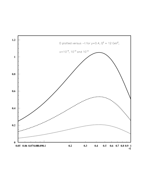
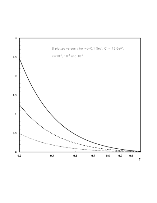
Figure 5.4: a) $D$ is plotted versus $-t$ for $x=10^{-4},10^{-3},10^{-2}$, $Q^{2}=12~{}\mbox{GeV}^{2}$, $B=5~{}\mbox{GeV}^{-2}$ and $y=0.4$. The solid curve is for $x=10^{-4}$, the dotted one for $x=10^{-2}$ and the dashed one for $x=10^{-3}$. b) $D$ is plotted versus $y$ for the same $x,Q^{2},B$ and $-t=0.1~{}\mbox{GeV}^{2}$

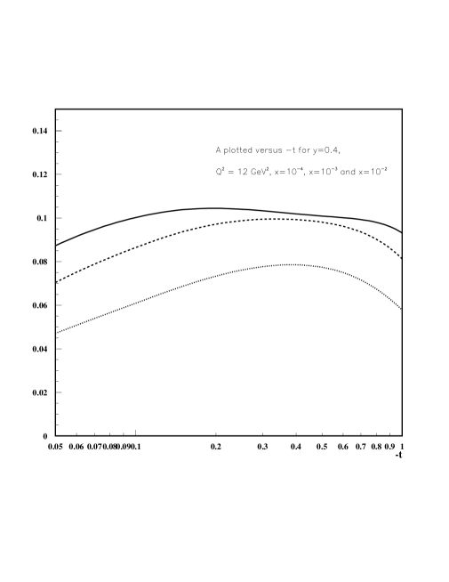
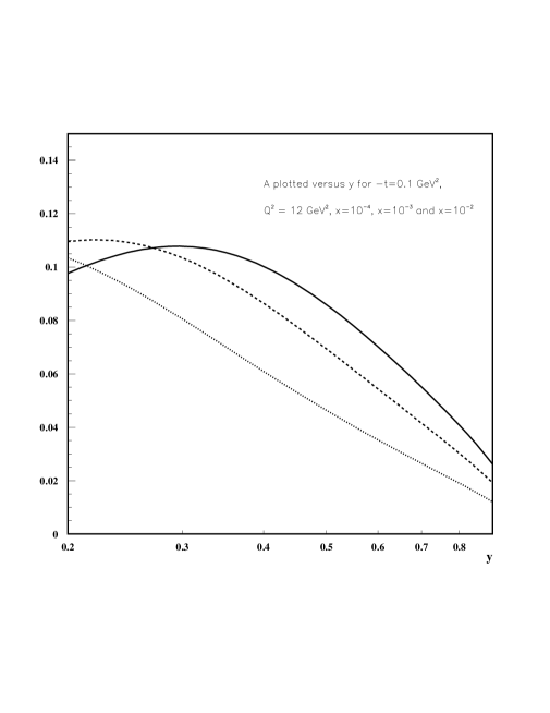
Figure 5.5: a) The asymmetry $A$ is plotted versus $-t$ for $x=10^{-4}$ (solid curve), $x=10^{-2}$ (dotted curve) and $x=10^{-3}$ (dashed curve) again for $Q^{2}=12~{}\mbox{GeV}^{2}$, $B=5~{}\mbox{GeV}^{-2}$ and $y=0.4$. b) $A$ is plotted versus $y$ for the same $x,Q^{2},B$ and $-t=0.1~{}\mbox{GeV}^{2}$.

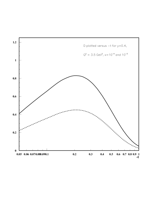
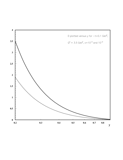
Figure 5.6: a) $D$ is plotted versus $-t$ for $x=10^{-4}$ and $10^{-3}$, $Q^{2}=3.5~{}\mbox{GeV}^{2}$, $B=8~{}\mbox{GeV}^{-2}$ and $y=0.4$. The solid curve is for $x=10^{-4}$, the dashed one for $x=10^{-3}$. b) $D$ is plotted versus $y$ for the same $x,Q^{2},B$ and $-t=0.1~{}\mbox{GeV}^{2}$

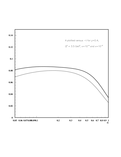
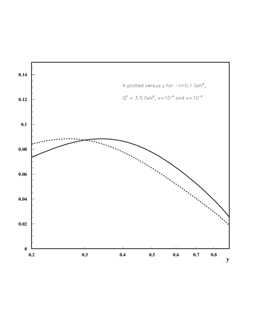
Figure 5.7: a) The asymmetry $A$ is plotted versus $-t$ for $x=10^{-4}$ (solid curve), $x=10^{-3}$ (dashed curve) again for $Q^{2}=3.5~{}\mbox{GeV}^{2}$, $B=8~{}\mbox{GeV}^{-2}$ and $y=0.4$. b) $A$ is plotted versus $y$ for the same $x,Q^{2},B$ and $-t=0.1~{}\mbox{GeV}^{2}$.

Chapter 6 DVCS in DIS at HERA - A Probe of Asymptotia

6.1 Introduction

In this chapter based on Ref. [82], we will attempt to answer one of the pressing questions of high-energy QCD: The energy dependence of the strong amplitude in the situation when one or both colliding systems have small size. It is generally agreed that the $x$-range currently available at HERA is not sufficient to test the current ideas about the onset of asymptotia via measurements of the parton densities.

At the same time, the experience in studies of soft processes tells us that the real part of the zero angle scattering amplitude, $\eta$, provides us, through the dispersion representation over the invariant energy of the collision, with information about the energy dependence of the cross section well beyond the energy where $\eta$ is measured. The reason for this is that $\eta$, the ratio of the real to imaginary part of the amplitude essentially measures the $\ln s$ derivative of the cross section [33]:

$$\eta=\frac{\pi}{2}\frac{d\ln(F_{2}(x,Q^{2}))}{d\ln(1/x)}.$$ (6.1)

One can also use derivative analyticity relations to derive a more accurate formula [33, 34], leading to

$$\eta=tan\left[{\pi\alpha\over 2}\right].$$ (6.2)

for $F_{2}(x,Q^{2})\propto x^{-\alpha}$.

In this chapter we propose a new methodology of investigating the energy dependence of high-energy processes through their real parts and also the shapes of nondiagonal parton distributions. We use DVCS as an example which offers us a direct way to study nondiagonal parton distributions, though their actual extraction from the data is not possible in DVCS due to the fact that the parton distributions depend on $y_{1}$ and $y_{2}=y_{1}-x$ which are dependent variables rather than independent as one would need and thus the inverse Mellin transform of the factorization formula cannot be found. The major new result of this chapter is that the current successful fits to the $F_{2N}(x,Q^{2})$ HERA data lead to qualitatively different predictions for the asymmetry, reflecting different underlying assumptions of the fits about the behavior of parton densities at $x$ below the HERA range.

A recent analysis in Ref.  [56] and the previous chapter have shown that DVCS studies at HERA are feasible and we made predictions for the expected DVCS counting rate compared to DIS as well as the asymmetry $A$ in the combined DVCS and Bethe-Heitler cross section for recent H1 data [76].

The chapter is structured as follows. In Sec. 6.2 we review the necessary formulas of Ref. [56] and the previous chapter for our analysis. In this context, the formula pertaining to the ratio of real to imaginary part of a scattering amplitude at small $x$ is of particular importance. We then present the different fits to $F_{2}(x,Q^{2})$ in Sec. 6.3 and present the different results for the asymmetry $A$ with respect to $t$ and $y$, at fixed $y$ and $t$ respectively. Sec. 6.5 contains our conclusions and outlook.

6.2 Relations between DVCS and DIS

In order to compute the asymmetry $A$, we need the ratio of the imaginary part of the DIS amplitude to the imaginary part of the DVCS amplitude and the relative DVCS counting rate $R_{\gamma}$, expected at HERA in the interesting kinematic regime of $10^{-4}<x<10^{-2}$ and moderate $Q^{2}$, i.e. , $3.5~{}\mbox{GeV}^{2}<Q^{2}<45~{}\mbox{GeV}^{2}$. The relative counting rate $R_{\gamma}$ is given by [56]

$$R_{\gamma}\simeq\frac{\pi\alpha}{4R^{2}Q^{2}B}F_{2}(x,Q^{2})(1+\eta^{2}).$$ (6.3)

where $R$ is the ratio of the imaginary parts of the DIS to DVCS amplitude as given in [56] , $B$ is the slope of the $t$ dependence (for more details see Ref. [56] and the previous chapter.) and $\eta$ is the ratio of real to imaginary part of the DIS amplitude, i.e. , $F_{2}(x,Q^{2})$, given by Eq. (6.1).

The asymmetry $A$ is given by [56]

$$A=\frac{\int_{-\pi/2}^{\pi/2}d\phi_{r}d\sigma_{DVCS+BH}-\int^{3\pi/2}_{\pi/2}d\phi_{r}d\sigma_{DVCS+BH}}{\int_{0}^{2\pi}d\phi_{r}d\sigma_{DVCS+BH}},$$ (6.4)

where $d\sigma_{DVCS+BH}$ is given by the sum of Eq. (5.36),(5.37),(5.40). As explained in [56] this azimuthal angle asymmetry is due to the sign change of the interference term in the combined DVCS and Bethe-Heitler cross section, when the angle $\phi_{r}$ is integrated over the upper hemisphere of the detector as compared to the integration over the lower hemisphere of the detector. Although the absolute value of the parton distributions cannot be extracted from DVCS, the shape of the distributions is nevertheless accessible since the real part of the DVCS amplitude is isolated through this asymmetry. Therefore, we investigate the influence of different $F_{2}$ fits on the asymmetry through the relative counting rate which is directly sensitive to the ratio of real to imaginary parts of $F_{2}$ as shown in Eq. (6.3).

6.3 The different fits to $F_{2}(x,Q^{2})$

In the calculation of the asymmetry $A$ we use the recent H1 data from Ref. [76] as previously used in Ref. [56], a logarithmic fit by Buchmüller et. al (BH) [78], the ALLM97 fit [79] and a leading order BFKL-fit [80] for illustrative purposes.

In the H1 data, $F_{2}$ behaves for small $x$ as $x^{-\lambda}$ and hence $\eta$ is just $\frac{\pi}{2}\lambda$ where $\eta^{2}=0.09-0.27$ in the $Q^{2}$ range given in the previous section. Note that $\eta$ has no $x$ dependence, for small enough $x$, and thus depends only on $Q^{2}$. This is not true for all of the other fits.

$F_{2}$ in the BH fit takes on the following form

$$F_{2}(x,Q^{2})=0.078+0.364\log(\frac{Q^{2}}{0.5~{}\mbox{GeV}^{2}})\log(\frac{0.074}{x}),$$ (6.5)

and hence we find for $\eta$

$$\eta=\frac{\pi}{2}0.364\log(\frac{Q^{2}}{0.5~{}\mbox{GeV}^{2}})/F_{2}(x,Q^{2}).$$ (6.6)

Note that this $\eta$ has not only the usual $Q^{2}$ dependence but depends rather strongly on $x$ also, which is not seen in the data for the slope of $F_{2}$.

In the ALLM97 fit $F_{2}$ at small $x$ takes on the following form

$$F_{2}(x,Q^{2})=\frac{Q^{2}}{Q^{2}+m_{0}^{2}}(F_{s}^{p}(x,Q^{2})+F_{2}^{R}(x,Q^{2})),$$ (6.7)

with

$$F_{2}^{P}(x,Q^{2}) = c_{P}(t)x_{P}^{a_{P}(t)}$$

$$F_{2}^{R}(x,Q^{2}) = c_{R}(t)x_{R}^{a_{R}(t)},$$ (6.8)

where

$$t=\ln\left(\frac{\ln\left(\frac{Q^{2}+Q_{0}^{2}}{\Lambda^{2}}\right)}{\ln\left(\frac{Q_{0}^{2}}{\Lambda^{2}}\right)}\right),$$ (6.9)

and

$$c_{R}(t) = 0.8017+0.97307t^{3.4942},$$

$$a_{R}(t) = 0.584+0.37888t^{2.6063},$$

$$c_{P}(t) = 0.28067+0.05776\left(\frac{1}{1+t^{2.1979}}-1\right),$$

$$a_{P}(t) = -0.0808+0.36732\left(\frac{1}{1+t^{1.1709}}-1\right).$$ (6.10)

$x_{P}$ and $x_{R}$ are given at small $x$ by

$$x_{P} = x(1+\frac{m_{P}^{2}}{Q^{2}}),$$

$$x_{R} = x.$$ (6.11)

$\Lambda^{2}=0.06527~{}\mbox{GeV}^{2}$, $m_{P}^{2}=49.457~{}\mbox{GeV}^{2}$, $Q_{0}^{2}=0.46017~{}\mbox{GeV}^{2}$ and $m_{0}^{2}=0.31985~{}\mbox{GeV}^{2}$. $\eta$ is then given by

$$\eta=-\frac{\pi}{2}\frac{a_{P}c_{P}x_{P}^{a_{P}}+a_{R}c_{R}x_{R}^{a_{R}}}{c_{P}x_{P}^{a_{P}}+c_{R}x_{R}^{a_{R}}}.$$ (6.12)

In the case of BFKL where $F_{2}\simeq x^{-\frac{4N_{c}\ln(2)\alpha_{s}}{\pi}}$ we find $\eta$ to be

$$\eta=\frac{\pi}{2}\frac{4N_{c}\ln(2)\alpha_{s}}{\pi}$$ (6.13)

with an $\alpha_{s}$ in leading order of

$$\alpha_{s}=\frac{4\pi}{3N_{c}\log\left(\frac{Q^{2}}{\Lambda^{2}}\right)}.$$ (6.14)

6.4 Results for the asymmetry $A$

In Fig. 6.1 - 6.3, we plot the asymmetry $A$ as a function of $t$ and $y$ for fixed $Q^{2}=12~{}\mbox{GeV}^{2}$, fixed $y=0.4$ and $-t=0.1~{}\mbox{GeV}^{2}$ and $x=10^{-4},~{}10^{-3},~{}10^{-2}$. The slope $B$ of the $t$-dependence for DVCS was taken to be $B=5~{}\mbox{GeV}^{-2}$ whereas for the Bethe-Heitler cross section we used the nucleon form factor as used in chapter 5. The counting rate $R_{\gamma}$ was appropriately adjusted for the different fits according to Eq. (6.3). The solid curves in Fig. 6.1 - 6.3 are our benchmarks.

Comparing the BH fit (dotted curves), against our benchmarks we find a strong $x$ dependence of the asymmetry in the BH fit as well as different shapes and absolute values. The strong $x$ dependence of the BH fit in the ratio of the real to imaginary part of $F_{2}$ will make it easy to distinguish this logarithmic fit from a power law fit which yields an $x$ independent $\eta$.

As far as the ALLM97 fit is concerned (short-dash curves), there is hardly a difference, as compared to the H1 fit in the asymmetry as a function of $t$ and $y$ in absolute value, shape and $x$ dependence, except for $x=10^{-2}$ but this is due to the approximations we made for $x_{P}$ and $x_{R}$ which are not that good anymore at $x=10^{-2}$.

If one compares the BFKL fit (dash-dot curves) to the H1 fit one sees immediately that the BFKL fit is totally off in almost all aspects and was only included here as an illustrative example, not as a serious fit.

6.5 Conclusions

In the above we have shown the sensitivity of the exclusive DVCS asymmetry $A$ to different $F_{2}$ fits and made comments on the viability of each fit. Note that even a fit which reproduces $F_{2}$ data, as well as its slope, in a satisfactory manner can be shown to lead to differences in the asymmetry shape. The sensitivity of the asymmetry to $y$ and $t$ will allow us, once experimentally determined, to make a shape fit and hence make a shape fit to nondiagonal parton distributions for the first time.

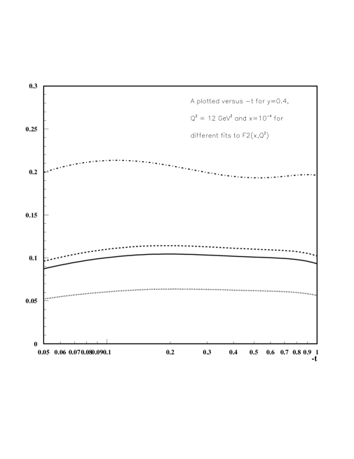
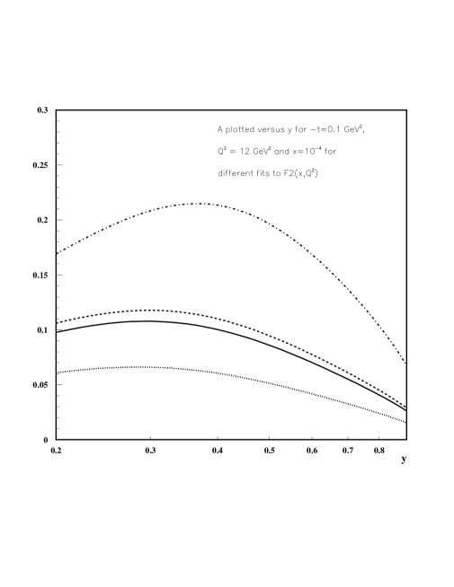
Figure 6.1: H1 fit (solid curve), the BH fit (dotted curve), ALLM97 fit (short-dash curve) and BFKL fit (dash-dot curve) for $x=10^{-4}$. a) Asymmetry $A$ versus $t$ for fixed $y=0.4$. b) Asymmetry $A$ versus $y$ for fixed $-t=0.1~{}\mbox{GeV}^{2}$.

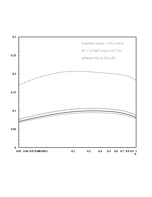
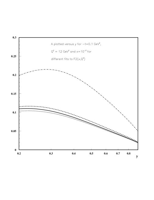
Figure 6.2: H1 fit (solid curve), the BH fit (dotted curve), ALLM97 fit (short-dash curve) and BFKL fit (dash-dot curve) for $x=10^{-3}$. a) Asymmetry $A$ versus $t$ for fixed $y=0.4$. b) Asymmetry $A$ versus $y$ for fixed $-t=0.1~{}\mbox{GeV}^{2}$

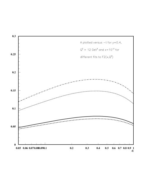
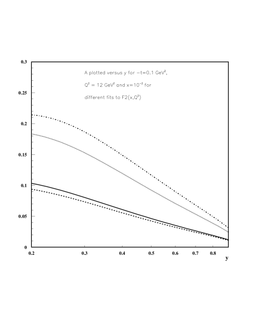
Figure 6.3: H1 fit (solid curve), the BH fit (dotted), ALLM97 fit (short-dash curve) and BFKL fit (dash-dot curve) for $x=10^{-2}$. a) Asymmetry $A$ versus $t$ for fixed $y=0.4$. b) Asymmetry $A$ versus $y$ for fixed $-t=0.1~{}\mbox{GeV}^{2}$

Appendix A Direct Estimation of Sizes of Higher-Order Graphs

A.1 Introduction

In this appendix, based on Ref. [83], we want to give concrete examples of distributional methods which were employed in an abstract way in chapter 4. The starting point for this appendix is formed by the following observations:

• The only (known) systematic method for calculating scattering in QCD is perturbation theory. (Lattice Monte-Carlo methods work in Euclidean space-time, and are excellent for calculating static quantities such as masses from first principles. But they are essentially useless when a calculation in real Minkowski space-time is needed.)

• In field theory, calculations beyond low orders of perturbation theory are computationally complex, both because the calculations of individual graphs are hard and because there are many different graphs.

• Hence it is important to make the most efficient use of low-order calculations.

Since the coupling in practical calculations is not very weak, the accuracy of predictions can be ruined by uncalculated higher-order terms. It follows that there is a need to estimate the sizes of the errors. For this one wants quick estimates of terms in perturbation theory. The computational complexity of the estimates should increase as little as possible with the size of the graphs. Indeed, our aim is that one only calculates integrals of the form

$$\int_{l}^{u}dx\,x^{n}\,\ln^{p}x.$$ (A.1)

With suitable methods:

• One can determine good values for renormalization and factorization scales, by asking how to minimize the error estimates.

• When the estimates get substantially larger than some appropriate “natural” size, one would get a diagnosis of a need for resummation of classes of higher-order corrections. The diagnosis would include an explanation of the large terms and thus indicate the physics associated with the resummation.

In this appendix, we explain how to start such a program. It builds on work first reported in Ref. [81]. Our methods treat properties of the integrands of Feynman graphs, and are therefore directly sensitive to the physics of the process being discussed. Some other treatments of these issues discuss the problems in terms of the mathematics of series expansions in general, without asking what is causing the graphs to be the sizes they are. A particular exception is the work of Brodsky, Lepage, and Mackenzie [84]. They use heavy quark loops to probe the actual momentum scales that dominate in a particular calculation; this is then used to provide a suitable value for the renormalization/factorization scale. But we believe that our methods provide a more direct route to answering the question of why the scales are what they are and why a calculation gives a particular order of magnitude. The issues addressed by methods involving the Borel transform and Padé summation address complementary issues [87].

Now, most cross sections in QCD cannot be directly computed by perturbation theory; this can only be used to compute the short-distance coefficients that appear in the factorization theorem. So we will also treat the specific problems that arise in estimating the sizes of the coefficient functions. These functions have the form of a sum over Feynman graphs (typically massless), with subtractions to cancel some infra-red (IR) divergences. Remaining IR divergences are cancelled between different graphs or between different final-state cuts. Two characteristic features appear. First, we can obtain estimates for sums of particular sets of graphs, but not for the individual graphs, which are divergent. Secondly, the coefficient functions are not in fact genuine functions. They are normally singular generalized functions (or distributions) and an estimate can only be made for the integral of a coefficient function with a smooth test function.

We show how to estimate the sizes of graphs by a direct examination of the integrands. An important part of our technique is an implementation of subtractions directly in the integrands, both for the subtractions that implement counterterms for ultra-violet (UV) renormalization and for the IR subtractions that are used in short-distance coefficient functions. In order to explain our ideas, we will examine two examples: (1) the one-loop self-energy graph in $(\phi^{3})_{4}$ theory, and (2) a particular set of graphs for the Wilson coefficient for deep-inelastic scattering. Our estimates are in the form of approximations to ordinary integrals that are absolutely convergent. This is in contrast to the original integrals, which are typically divergent in the absence of a regulator. Thus a by-product of our work will be algorithms for computing graphs numerically in Minkowski space-time, which may have relevance to work such as Ref. [88]. As an illustration of how estimations can be carried out, even analytically, for a measurable quantity, we will estimate the size of the Wilson coefficient for the structure functions $F_{T}$ and $F_{L}$ in the last section.

A.2 Euclidean self-energy in $\phi^{3}$ theory

In this section, we give a representation of the one-loop self-energy graph of Fig. A.1 in $\phi^{3}$ theory in four dimensions. A particular renormalization scheme is used, which we relate to ordinary $\overline{{\rm MS}}$ renormalization. Then we show how to estimate the size of the graph from elementary integrals and hence how to choose the renormalization scale suitably.

Figure A.1: One-loop self-energy graph.

A.2.1 Renormalization

The only complication in computing the graph of Fig. A.1 is its UV divergence, given that we choose to work in Euclidean space. We give a representation of the graph that is an absolutely convergent integral over the loop momentum itself in four dimensions and in which the renormalization is explicitly “minimal”. This last term means that the counterterm for the (logarithmic) divergence is independent of the mass and the external momentum. It is a very useful property when one wants to take zero-mass limits, etc. For a general divergence, the counterterm would be polynomial in masses and external momenta.

Our representation of the graph is:

$$I(p)=\frac{1}{2}\frac{g^{2}}{(2\pi)^{4}}\int d^{4}k\left\{\frac{1}{(k^{2}+m^{2})\,\left[(p-k)^{2}+m^{2}\right]}-\frac{\theta(k>\mu_{c})}{k^{4}}\right\}.$$ (A.2)

We recognize in the integrand a term that is given by the usual Feynman rules (in Euclidean space-time), and a subtraction term. The subtraction term is the negative of the asymptote of the first term as $k\to\infty$, so we term our procedure “renormalization by subtraction of the asymptote”. A cut-off is applied to prevent the subtraction term giving an IR divergence at $k=0$; the cut-off does not affect the $k\to\infty$ behavior and therefore does not affect the fact that the UV divergence is cancelled. To see that Eq. (A.2) is equivalent to standard renormalization, one simply applies a UV regulator, after which each term can be integrated separately. The first term is the unrenormalized graph and the second term is a $p$-independent counterterm.

Evidently, the integral is absolutely convergent, and can therefore be computed by any appropriate numerical method. (It can also be evaluated analytically. But this is not interesting to us, since we wish to obtain methods that work for integrals that are too complicated for purely analytic methods to be convenient or useful.)

The counterterm is in fact the most general one that is independent of $m$ and $p$, since any other renormalization counterterm can differ only by a finite term added to the integral that is independent of $m$ and $p$, and a change of the cut-off $\mu_{c}$ is equivalent to adding such a term. We can relate the counterterm to the commonly used $\overline{{\rm MS}}$ one simply by computing the counterterm alone, with dimensional regularization:

$$\mbox{standard prefactor}\times\int_{|k|>\mu_{c}}d^{n}k\,\frac{1}{k^{4}}.$$ (A.3)

The result is that setting $\mu_{c}$ equal to the scale $\mu$ of the $\overline{{\rm MS}}$ scheme gives exactly $\overline{{\rm MS}}$ renormalization. In general, we would find that $\mu_{c}$ would be a factor times $\mu$, or equivalently that we should set $\mu_{c}=\mu$ and then add a specific finite counterterm to the graph.

Notice that the integral to relate our renormalization scheme to the $\overline{{\rm MS}}$ scheme is algorithmically simpler to compute analytically than the original integral. There is always the possibility of adding finite counterterms. Moreover, the precise form of the cut-off is irrelevant to the general principles. One can, for example, change the sharp cut-off function $\theta(k>\mu_{c})$ to a smooth function $f(k/\mu_{c})$ that obeys $f(\infty)=1$ and $f(0)=0$. Such a function would probably be better in numerical integration.

Of course, our method as stated is specific to one-loop graphs. But it is an idea that has been generalized [89, 90] to higher orders.

A.2.2 Estimate

We now show how to estimate the size of the integral Eq. (A.2). To give ourselves a definite case, let us choose $p^{2}\leq m^{2}$. We obtain the estimate as the sum of contributions from $k<m$ and from $k>m$. Since the renormalization counterterm is designed to subtract the $k\to\infty$ behavior of the unrenormalized integrand, we regard it as a $\delta$-function at infinity and therefore to be associated completely with the $k>m$ term in our estimate.

In the region $k<m$, our estimate is obtained by replacing each propagator by $1/m^{2}$ so that

Contribution from $$k<m \simeq \frac{g^{2}}{32\pi^{4}}\int_{k<m}d^{4}k\frac{1}{m^{4}}$$ (A.4)

$$= \frac{g^{2}}{64\pi^{2}}.$$

This factor is the product of $g^{2}/32\pi^{4}$ for the prefactor and $\pi^{2}/2$ for the volume of a unit 4-sphere. As advertised, we have had to calculate no integral that is more complicated than a simple power of $k$. The approximation of replacing the propagators by $1/m^{2}$ leads us to an over-estimate of the integral, but not by a great factor, since we are in a region of small momentum.

The estimate for $k>m$ is obtained by replacing the propagators by their large $k$ asymptote:

Contribution from $$k>m \simeq \frac{g^{2}}{32\pi^{4}}\int_{k>m}d^{4}k\left[\frac{1}{k^{4}}-\frac{\theta(k>\mu_{c})}{k^{4}}\right]$$ (A.5)

$$= \frac{g^{2}}{32\pi^{4}}2\pi^{2}\left[\int_{m}^{\infty}\frac{dk}{k}-\int_{\mu}^{\infty}\frac{dk}{k}\right].$$

Since we are taking the difference of two terms, we must be careful about the errors, which are of order

$$\int_{k>m}d^{4}k\frac{m^{2}}{k^{6}}=\frac{g^{2}}{32\pi^{2}}.$$ (A.6)

To understand the structure of the result, let us examine how the original integral (A.2) appears after integrating over the angle of $k$:

$$\frac{g^{2}}{16\pi^{2}}\int_{0}^{\infty}\frac{dk}{k}\left[A(k,p,m)-\theta(k>\mu_{c})\right].$$ (A.7)

The function $A$ is the angular average of $k^{4}$ times the two propagators. It approaches 0 as $k\to 0$, so that the integral is convergent there, and it approaches unity as $k\to\infty$, which would give a UV divergence were it not for the subtraction.

Figure A.2: (a) Scaled integrand for unrenormalized self-energy graph. (b) Subtraction term. (c) Total if $\mu\sim m$. (d) Total if $\mu\gg m$.

We can represent this situation by the graphs of Fig. A.2. The transition region for the unsubtracted integrand, where it changes from being 0 to 1, is around $k=m$, to within a factor of 2 or so; this is evident by examining the denominators. By setting $\mu_{c}$ to be $m$ to within a factor of 2, we achieve the following:

• The integrand is less than unity everywhere.

• It is concentrated in a shell of thickness of order $m$ around $k=m$.

Thus we can say that the natural size of the graph is the product of

• The prefactor $g^{2}/32\pi^{4}$.

• The surface area of a unit 4-sphere: $2\pi^{2}$.

• The width of the important region, about unity, in units of $m$.

• A factor of $m$ to the dimension of the integral, i.e., 1.

• A factor less than unity, say $1/2$, to allow for the fact that, after subtraction, the integrand in Eq. (A.7) is smaller than unity and that there is a cancelation between negative and positive pieces.

That is, the natural size is $g^{2}/32\pi^{2}$, if $\mu$ is reasonably close to $m$.

If $\mu$ is not close to $m$, then we get a long plateau in the integrand—see Fig. A.2. The height of the plateau is unity, and its length is $\ln(\mu/m)$ to about $\pm 1$ in units of $\ln k$. This clearly gives a larger-than-necessary size, and an optimal choice of the $\overline{{\rm MS}}$ scale is around $m$.

One should not expect to get an exact value for the scale $\mu$. A physical quantity in the exact theory is independent of $\mu$, and any finite-order calculation differs from the correct value by an amount whose precise value is necessarily unknown until one has done a more accurate calculation. If one is able to estimate the size of the error, as we are proposing, then an appropriate value of $\mu$ is one that minimizes the error. Given the intrinsic imprecision of an error estimate, there is a corresponding imprecision in the determination of $\mu$. One can expect to identify, without much work, an appropriate scale $\mu$ to within a factor 2, and, with a bit more work, to within perhaps $50\%$. These estimates just come from asking where the transition region in the integrand is, and by then obtaining an answer by simple examination of the integrand. But one cannot enter into a religious argument of the wrong kind as to whether the correct scale is $1.23m$ as opposed to $1.24m$, for example. By definition an error estimate is approximate.

Since we have not yet investigated how to estimate even higher-order graphs, we are making the reasonable conjecture that the properties of graphs do not change rapidly with order. Then our estimate that $\mu$ should be close to $m$ will ensure that higher-order graphs are of the order of their natural size.

A.2.3 Implication for QCD

The same arguments applied to similar graphs in QCD show that the natural expansion parameter in QCD is

$$\frac{\alpha_{s}}{4\pi}\times(\mbox{group theory})\times(\mbox{factor for multiplicity of graphs}).$$ (A.8)

These arguments rely on being able to show that in the dominant part of the range of integration all lines have approximately a particular virtuality and that the relevant range of integration is a corresponding volume of momentum space.

In the general case we cannot expect to get a much smaller result, but we can expect that in some situations the properties of the dominant integration region(s) will not be so good. So what we need to do next is to analyze more interesting graphs in QCD. This we will do in the next section.

In general, when we get corrections in QCD that are substantially larger than the natural size given above, it must be either because the integrand is excessively large, or because there is no single natural scale, or because we have not chosen a good scale. If the integrand is especially large relative to the natural unit, or if there is no single natural scale, then we should investigate in more detail the reasons, and derive something like a resummation of higher-order corrections [91]. In precisely such situations, one does indeed have to compute high-order graphs. At the same time, there is no need to compute the complete graphs in all their gory detail, but only their simple parts.

A.3 Wilson coefficient for deep-inelastic scattering

The factorization formula for the leading-twist part of a deep-inelastic structure function $F(x)$ is

$$F(x)=\int\frac{d\xi}{\xi}f(\xi)\hat{F}(x/\xi).$$ (A.9)

Here, $f(\xi)$ is a parton density, and $\hat{F}$ is the short-distance coefficient (“Wilson coefficient”). We have suppressed the indices for the different structure functions ($F_{1}$, $F_{2}$, etc.) and for the parton flavor. The coefficient function $\hat{F}(x/\xi)$ is obtained from Feynman graphs for scattering on a parton target with momentum $\xi p$, where $p$ is the momentum of the hadron target. Subtractions for initial-state collinear singularities are applied to the Wilson coefficient and the massless limit is taken.

Figure A.3: The cuts of a one-loop graph for the Wilson coefficient for deep-inelastic scattering.

As an example, we will examine the contribution to the Wilson coefficient from the diagrams in Fig. A.3. These diagrams are the two possible cuts of a particular uncut one-loop graph, and since we will need to use a cancelation of final-state interactions, we must consider the sum of the two cut graphs as a single unit. Note:

• We will apply a subtraction to cancel the effect of initial-state collinear interactions where the incoming quark splits into a quark–gluon pair which are moving almost parallel to the incoming particle.

• There will be soft-gluon interactions and collinear final-state interactions. These will cancel after the sum over cuts. (In a more general situation, a sum over a gauge-invariant set of graphs is necessary to get rid of all soft-gluon interactions.)

• The Wilson coefficient is a distribution (or generalized function) rather than an ordinary function of $x/\xi$. Thus it is useful to discuss only the size of the coefficient after it is integrated with a test function, but not the size of the unintegrated coefficient function. The parton density $f(\xi)$ provides a ready-made test function that has a physical interpretation.

• The first graph of Fig. A.3, which has a virtual gluon, has a 4-dimensional integral, but the second graph, with a real gluon, has only a 3-dimensional integral. Thus the cancelations associated with the sum over cuts can only be seen after doing at least a 1-dimensional integral.

Figure A.4: Space-time structure of deep-inelastic scattering, in the center-of-mass frame of the virtual photon and the struck quark. The solid line is the almost (light-like) world line of the incoming quark. The dashed line is the world line of the single struck quark in the lowest-order (Born) graph for the hard scattering.

It is useful to visualize the process in space-time, Fig. A.4, and to use light-front coordinates $(+,-,T)$ (defined by $V^{\pm}=(V^{0}\pm V^{3})/\sqrt{2}$). Our axes are such that the incoming momenta for the hard scattering are:

$$\xi p^{\mu}=(\xi p^{+},0,{\bf 0}_{T}),~{}~{}~{}~{}q^{\mu}=\left(-xp^{+},\frac{Q^{2}}{2xp^{+}},{\bf 0}_{T}\right).$$ (A.10)

Also, we find it convenient to parameterize the gluon momentum in Fig. A.3 in terms of two longitudinal momentum fractions, $u$ and $z$, and a transverse momentum ${\bf k}_{T}$, as follows:

$$k^{\mu}=(u\xi(1-z)p^{+},\,zq^{-},\,{\bf k}_{T}).$$ (A.11)

Thus $z$ is exactly the fraction of the total incoming minus component of momentum that is carried off by the gluon, while $u$ is a scaled fraction of the plus component. The scaling is somewhat unobvious, but it has the effect that positive energy constraints on the final state restrict each of $u$ and $z$ to range from 0 to 1.

Now we summarize how the calculation of the real and virtual graphs and of the subtraction graphs [92], contributing to the Wilson coefficients, is to be carried out:

• Using the Feynman rules for cut diagrams, we write down the momentum integral with the appropriate $\delta$-functions. Then we contract the trace over Dirac matrices with the appropriate transverse, longitudinal or asymmetric tensor on the photon indices to obtain the structure function $F_{1}$, $F_{2}$, etc. For the sake of a definite simple example we choose to contract with $-g_{\mu\nu}$, which in fact gives the combination $3F_{1}-F_{2}/2x$.

• We express the results of the calculations in terms of the light-cone components of $k$ (the internal gluon momentum), of $p$ (the incoming quark momentum), and of $q$ (the incoming photon momentum).

• In the graphs with real gluon emission, we use the two $\delta$-functions to perform the integrals over ${\bf k}_{T}$ and over the fractional momentum $\xi$ entering from the parton density. This leaves a 2-dimensional integral.

• In the virtual graphs, we use the one $\delta$-function to perform the integral over the fractional momentum $\xi$ entering from the parton density. We then perform the ${\bf k}_{T}$ integral analytically. Again we have a 2-dimensional integral.

• We change the integration variables to the scaled dimensionless variables $u$ and $z$ defined in Eq. (A.11). This gives us an overall factor, just like the $g^{2}/16\pi^{2}$ in the self energy, times an integral over roughly the unit square in $u$ and $z$.

Figure A.5: Integration region and position of singularities for Fig. A.3(a).

A.3.1 Real gluon

For the real gluon graph Fig. A.3(a) it is well known that the integrand has the following singularities in the massless limit:

• Initial-state collinear singularity on $z=0$.

• Final-state collinear singularity on $u=0$.

• Soft singularity $k=0$ at the intersection of the previous two singularities, i.e., at $u=z=0$.

(See Fig. A.5.) In accordance with the standard recipe for constructing the Wilson coefficient, we subtract the initial-state collinear singularity. The subtraction term itself has a UV divergence, which we choose to cancel by using the same method as we used for the UV divergence of the self-energy graph. This gives

$$\frac{g^{2}}{8\pi^{2}}C_{F}\int_{0}^{1}dz\int_{0}^{1-x}du\,f\left(\frac{x}{1-u}\right)\;\left[\frac{1-z}{zu}-\frac{\theta(z<z_{\rm cut})}{zu}\right].$$ (A.12)

The cut-off $z_{\rm cut}$ on the subtraction term is analogous to the cut-off $\mu_{c}$ we used for the UV counterterm for the self-energy graph. The value of $z_{\rm cut}$ needed to reproduce the $\overline{{\rm MS}}$ prescription can be found by a simple calculation from the Feynman rules for parton densities. But we will not use this result here. Rather, we will aim at calculating an appropriate value for $z_{\rm cut}$ to keep the one-loop correction down to a “normal size” (and, most importantly, whether it is possible to find such an appropriate value at all). This effectively amounts to a choice of factorization scheme. Once a suitable value for $z_{\rm cut}$ has been obtained, it is a mechanical matter to translate it to a value for $\mu_{\overline{{\rm MS}}}$ (or to a value of the scale $\mu$ in any other chosen scheme). The calculation may also result in a need for an extra finite counterterm.

The subtraction in Eq. (A.12) has evidently accomplished its purpose of cancelling the initial-state singularity. But we are still left with the singularity on the line $u=0$. This singularity will cancel against a singularity in the virtual graph, as we will now see.

A.3.2 Sum of virtual and real graphs

Next we compute the virtual graph of Fig. A.3(b), following the same line as in the previous subsection. We will construct an integral in the same variables as the real graph. The reason why we do this is that the cancelation of the divergence at $u=0$ will be point-by-point in the integrand. This can be seen from the proof by Libby and Sterman [60]. They treat a general case of final-state interactions, of which our example is a particular case. They first treat one integration analytically, with the aid of the mass-shell conditions for the final state, in such a way that the integrations for graphs related by different positions of the final-state cut then have the same dimensions. After that, the cancelation between the different graphs is point-by-point in the integrand.

This implies that we need to perform the $\xi$ and ${\bf k}_{T}$ integrals. We do the convolution with $\xi$ by the mass-shell $\delta$-function, which now gives $\xi=x$. Then we do the ${\bf k}_{T}$-integral analytically. (This is not the most trivial integral, but it works conveniently with our choice of variables.) An example of the type of integral encountered is:

$$\int_{0}^{\infty}\frac{dk_{T}^{2}}{[Q^{2}(z-1)u-k_{T}^{2}+i\epsilon]\,[Q^{2}(u-1)z-k_{T}^{2}+i\epsilon]\,[Q^{2}uz-k_{T}^{2}+i\epsilon]}.$$

In the virtual case, no longer does a positive energy condition restrict the range of $u$ and $z$. Nevertheless, it is convenient to split up the result into a piece inside the square $0\leq u,z\leq 1$ and a piece from outside the square. It is sufficient to examine the contribution within the square. After subtracting the collinear singularity and adding the result from the real graph we get

$$\frac{g^{2}}{8\pi^{2}}C_{F}\int_{0}^{1}\int_{0}^{1}du\,dz\;\left[f\left(\frac{x}{1-u}\right)-(1-u)f(x)\right]\;\left[\frac{1-z}{zu}-\frac{\theta(z<z_{\rm cut})}{zu}\right]$$

$$+\ \mbox{contribution from {\em outside} $0\leq u,z\leq 1$}.$$ (A.13)

The UV divergence ($k\to\infty$) is from outside the square and is cancelled by subtractions just as for the self-energy graph.

We see that the singularity at $u=0$ for fixed $z$ has cancelled, even at the intersection of the two singular lines. However, how good the cancelation is depends on the test function. If $f(x)$ is slowly varying, the cancelation is good over a wide range of $u$. But if $f(x)$ is steeply falling as $x$ increases, the cancelation is good only over a narrow range of $u$, and we are left with an integrand that behaves like $1/u$ for larger $u$. For fixed $z$ we then have an integrand like that in Fig. A.6.

Figure A.6: The integrand of Eq. (A.13) as a function of $u$ at fixed $z$ when $f(x)$ is a steeply falling function of $x$.

This kind of behavior is quite typical when singularities are cancelled between different graphs with different final states. The integrand is a non-trivial distribution, and how good the cancelation of the singularity is depends on properties of the test function. The cancelation only occurs after integration over a range of final states. This is in distinct contrast with the case of the initial-state singularity for which we have constructed an explicit subtraction. The cancelation of the $z\to 0$ singularity occurs before the integration with the test function.

Immediately we also get complications in computing the typical size of the graph. In particular, when $f(x)$ is steeply falling, we should therefore expect a size for the integral that is much larger than the natural size we defined earlier.

A.3.3 Estimate of size

First, as a benchmark case, let us assume that $f(x/(1-u))$ is slowly and smoothly varying when $u$ increases from 0 to $1/2$, and that $z_{\rm cut}$ is around $1/2$. Then the size of (A.13) can be estimated as

$$\frac{g^{2}}{8\pi^{2}}\times\left(\mbox{group theory}\right)\times\left(\mbox{area of unit square in $(u,z)$}\right)\times f(x)\simeq\frac{g^{2}}{6\pi^{2}}f(x).$$ (A.14)

A way of obtaining this result with the same method as we used for the self-energy is to write

$$\frac{g^{2}}{(2\pi)^{4}}C_{F}\times\Bigg{(}\mbox{range of $k$, i.e., $2\pi^{2}Q^{4}$}\Bigg{)}\times\Bigg{(}\mbox{size of integrand, $\displaystyle\frac{f(x)}{Q^{4}}$}\Bigg{)}.$$ (A.15)

Given that the lowest-order graph is $f(x)$, and that the integrand varies in sign, all this implies that the contribution of this graph (with all the cuts and subtractions) is probably somewhat smaller than $g^{2}/6\pi^{2}$ times the lowest-order graph. In other words, the simplest estimate for the graphs, Eq. (A.8), is a valid estimate in this situation.

There are a modest number of graphs, so this result would have very nice implications for the good behavior of perturbation theory: the real expansion parameter of QCD would be $\alpha_{s}/\pi$, which is a few per cent in many practical situations.

Unfortunately, the conclusion is vitiated when $f(x)$ is steep, as is often the case. Consider the parton density factor times the $1/u$ factor, relative to the lowest-order factor $f(x)$. In the limit $u\to 0$, this is

$$\frac{f\left(\frac{x}{1-u}\right)-f(x)}{uf(x)}\sim\frac{xf^{\prime}(x)}{f(x)}.$$ (A.16)

This factor should be of order unity, if the previous estimate of the size, Eq. (A.14), is to be valid.

But if the logarithmic derivative $xf^{\prime}(x)/f(x)$ is much bigger than 1, then we have to change our estimates. Consider a typical ansatz for a parton density:

$$f(x)\propto(1-x)^{6},$$ (A.17)

for which

$$\left|\frac{xf^{\prime}}{f}\right|=\frac{6x}{1-x}.$$ (A.18)

This is 6 when $x=1/2$, and goes to infinity as $x\to 1$. Clearly our estimate in Eq. (A.14) is bad. Moreover the $u\to 0$ estimate, Eq. (A.16), is only approximately valid when $f(x)$ does not change by more than a factor 2 (roughly). Once $u$ gets larger than the inverse of the logarithmic derivative, the $f(x/(1-u))$ term in Eq. (A.13) is no longer important, and we get the result pictured in Fig. A.6: we have basically a $1/u$ form with a cut-off at small $u$. This is a recipe for a large logarithm, with the argument of the logarithm being the large logarithmic derivative.

To make the estimate, it is convenient to define

$$\delta u=-\frac{f(x)}{2f^{\prime}(x)x}.$$ (A.19)

From Eq. (A.16), we see that $\delta u$ is approximately the change in $u$ to make $f(x/(1-u))$ fall by a factor of 2. We interpret $\delta u$ as the value of $u$ at which the final-state cancelations become “bad”.

Next we note that for normal parton densities $f(x)$ is a decreasing function of $x$. So a simple useful estimate can be made by making the following approximation:

$$f\left(\frac{x}{1-u}\right)\simeq\left\{\begin{array}[]{l l}\displaystyle f(x)\left[1-\frac{u}{2\delta u}\right]&{\rm if~{}}u<2\delta u,\\ 0&{\rm if~{}}u>2\delta u\end{array}\right..$$ (A.20)

Therefore, in Eq. (A.13), we can replace $\int_{0}^{1}\frac{du}{u}f(x/(1-u))$ by $\int_{0}^{2\delta u}\frac{du}{u}f(x)$.

Our estimate for Eq. (A.13) is the sum of contributions from the following regions:

• $0<u<2\delta u$: The value of the integrand is about $-f(x)/2\delta u$ times a function of $z$. For good choices of $z_{\rm cut}$, the function of $z$ is less than about unity, but with an indefinite sign. Thus we obtain a contribution of about $f(x)$ in size.

• $2\delta u<u<1$: The integrand is now approximately $-f(x)/u$, again times a mild function of $z$. We therefore obtain a contribution of about $f(x)\ln(1/2\delta u)$.

• Exterior of unit square: Here, the only contribution is from the virtual graph, and we have no final-state singularity. Hence the naive estimate of unity is valid. (The precise value, when $\mu=Q$, is in fact somewhat larger.)

All of these are to be multiplied by the prefactor $g^{2}C_{F}/8\pi^{2}$. So we obtain a total contribution of

$$\frac{g^{2}}{8\pi^{2}}C_{F}f(x)\left[\pm 2\pm\ln\left(\frac{1}{2\delta u}\right)\right],$$ (A.21)

where each term represents an estimate, valid up to a factor of 2 or so. The contributions from within the unit square may have either sign, depending on the cut in the collinear subtraction, while the contributions from outside the unit square, from virtual graphs only, have a negative sign. As an explicit indication that our estimates are valid for the sizes but not the signs of the graphs, we have inserted a $\pm$ sign in front of each term. This estimate assumes that renormalization of the UV divergence of the virtual graph is done at the natural scale $\mu\simeq Q$, and that renormalization of the parton densities is done so that it corresponds to $z_{\rm cut}$ of about 1/2. It also assumes that $f(x)$ falls steeply enough for $\delta u$ to be less than about 1, as is typically true.

A.3.4 Interpretation

It is obvious that there is a logarithmic enhancement in Eq. (A.21) whenever $\delta u$ is small. Our calculation is, of course, no more than a rederivation of the standard observation that there are large logarithms in the $x\to 1$ region. What our derivation adds is to show that it is not so much the limit $x\to 1$ that is causing the problem as the steepness of the parton densities. Moreover we have given a numerical criterion for when the correction begins to be larger than what we called the natural size for higher-order corrections. In other words we have shown how to estimate the constant term that accompanies the logarithm. Moreover this is all presented in the context of a general method for obtaining estimates of the sizes of graphs.

It is perhaps clear that, with sufficient foresight, one could have predicted the large corrections merely from the observation that the derivation of the factorization theorem requires the cancelation of final-state divergences between different final states.

There is in fact another source of large corrections that will make its effect felt in even higher order. This is a mismatch in the scales needed for renormalizing the parton densities. We have renormalized these by using a value of $z_{\rm cut}$ that must be about 1/2 to avoid making the contribution of the graph unnecessarily large. In the case of the real graph, we can translate this to a scale of transverse momentum by using the mass-shell condition for the gluon:

$$k_{T}^{2}=Q^{2}uz(1-z)\frac{\xi}{x}=Q^{2}\frac{uz(1-z)}{1-u}.$$ (A.22)

Evidently, whenever small values of $u$ are important, small values of $k_{T}$ (relative to $Q$) will be important. This does not affect our one-loop calculation. But in higher-order correction, the virtuality of some internal lines will be controlled by the value of $k_{T}$, and hence there will be mismatches between the scales needed at different steps in the calculation.

Once one has diagnosed the problem, we see that a proper solution lies in more accurately calculating the form of the Wilson coefficient near its singularity. This subject goes under the heading of resummation of large corrections [91].

A.4 More detailed estimation of $F_{T,L}$ to one-loop order

In the following we will estimate the sizes of the one-loop corrections to the structure functions $F_{T}$ and $F_{L}$ without doing actual calculations of Feynman diagrams by giving a recipe of how to construct the estimates from general principles and kinematic considerations. However, we will present the recipe in the context of an actual set of Feynman graphs. By using the calculations of the graphs in Sec. A.5, we will verify that these “simple-minded” estimates are actually valid.

One obtains $F_{T,L}$ from the well-known hadronic tensor $W^{\mu\nu}$ by projecting out the “transverse” and “longitudinal” pieces via:

$$F_{T}=-g_{\mu\nu}W^{\mu\nu} = 3F_{1}-\frac{F_{2}}{2x}$$

$$F_{L}=\frac{Q^{2}p_{\mu}p_{\nu}}{p\cdot q^{2}}W^{\mu\nu} = -F_{1}+\frac{F_{2}}{2x},$$ (A.23)

which give, for example,

$$F_{1}=\frac{1}{2}\left[-g_{\mu\nu}-\frac{Q^{2}p_{\mu}p_{\nu}}{p\cdot q^{2}}\right]W^{\mu\nu}.$$ (A.24)

A.4.1 Estimation of $F_{L}$

The recipe for estimating $F_{L}$ is the following:

• The singularities we encounter (UV, collinear and soft) are all in the form of a factor times the Born graph, and the Born graph has no longitudinal part. Therefore the one-loop graphs for $F_{L}$ have no UV, soft or collinear singularities.

• Since the parton densities are falling with increasing $x$, the size of a graph is:

  $$\frac{g^{2}}{8\pi^{2}}\times C_{F}\times f(x)\times\mbox{{\rm range of $u$}}\times\mbox{{\rm range of $z$}}.$$ (A.25)

• The range of $z$ is 1.

• The range of $u$ is $\delta u$.

It is elementary to show that the self-energy and vertex graphs (whether real or virtual) give a zero contribution to $F_{L}$. Therefore, our result for $F_{L}$ is:

$$F_{L}=\frac{g^{2}}{6\pi^{2}}f(x)\delta u.$$ (A.26)

Let us now check whether our intuition has guided us in the right way. We use Eq. (A.36) for the contribution to the coefficient function for $F_{L}$. We approximate the $u$ integral by

$$\int duf\left(\frac{x}{1-u}\right)\simeq\delta uf(x),$$ (A.27)

which is appropriate for a typical parton density, which falls with increasing $x$. The $z$ integral gives a factor $1/2$, and we recover Eq. (A.26), which we obtained by more general arguments.

Notice that $F_{L}$ is generally rather smaller than what we have termed the natural size, because of the $\delta u$ factor: i.e., because of the restricted phase space available. There are no enhancements due to final-state singularities.

Our estimation methods can be applied in two ways. One is to estimate the graphs without having explicit expressions for the graphs; one just searches for the possible singularities that would prevent the natural size of a graph from being its actual size. The second way of using the methods is to examine the expressions for graphs with the knowledge of the singularity and subtraction structure and to perform a more direct estimate of the sizes. This is useful since the integrals must often be performed numerically, e.g., whenever one convolutes with parton densities that are only known numerically. Additional information that is now obtained concerns the typical virtualities, etc., of the internal lines of the graphs (compare Neubert’s work [86]). This enables a diagnosis to be made of the extent to which a problem is a multi-scale problem and therefore in need of resummation.

A point that we have not addressed is the estimation of the size of the trace of a string of gamma matrices, for example. In the standard formula for such a trace involves a large number of terms. Nevertheless, it is evident from the above calculations that there are cancelations. The final result is that we obtain, relative to corresponding numbers for a scalar field theory, a small factor (1 to 4) times a standard Lorentz-invariant quantity for the process.

Evidently, more work on this subject is needed. But the issue of the size of the numerator factors from traces, etc., affects completely finite quantities, such as the one-loop coefficient function for $F_{L}$, just as much as quantities with divergences that are cancelled. However, it is the latter quantities that have the potential for especially large corrections. Numerator factors result in magnitudes common to all graphs.

A.4.2 Estimation of $F_{T}$

We have already calculated one graph, Fig. A.3, for $F_{T}$, so we only need to summarize the method and apply it to the remaining graphs. The general procedure is:

• Since we have singularities in our graphs, they have to be cancelled. In Wilson coefficients such as we are calculating, there are explicit subtractions for the collinear initial-state singularities. Then there are explicit subtractions for UV divergences (both those associated with the interactions and those needed to define the parton densities and that therefore enter into the initial-state subtractions). Finally there are final-state singularities that cancel between real and virtual graphs.

• We consider separately the integrations inside and outside the square $0<u,z<1$.

• A term of the order of the natural size arises from outside the square $0<u,z<1$. This comes from purely virtual graphs, with their collinear subtraction.

• Inside the square, a real graph without a final-state singularity contributes an amount of the order of the natural size times $\delta u$. This reflects the restriction on the range of integration imposed by the parton density.

• Similarly a virtual graph without a final-state singularity contributes a term of the natural size.

• Finally, the sum of real and virtual graphs with a final-state singularity contributes a term of the order of the natural size enhanced by a factor $2+\ln(1/2\delta u)$, just as in our estimate of Fig. A.3.

We have the graphs of Fig. A.3, their Hermitian conjugates, the cut and uncut self-energy graph of Fig. A.7, below, and the ladder graph, Fig. A.8. Since $\delta u\leq 1$ typically, the ladder graph gives a small contribution, and it is sufficient to multiply the estimate of the Fig. A.3 by 3:

$$F_{T}=\frac{g^{2}}{2\pi^{2}}f(x)\left[2+\ln\left(\frac{1}{2\delta u}\right)\right].$$ (A.28)

To see how this compares with the results from the actual graphs, we use those in Sec. A.5.

The cut and uncut self-energy graphs, Fig. A.7 below, have final-state singularities, as can be seen in Eq. (A.34). We found it convenient to use $z$ and $k_{T}$ as integration variables. There is a singularity at $k_{T}=0$ in each individual graph. In analogy to the definition of $\delta u$, Eq. (A.19), we define

$$\delta k_{T}^{2}=\frac{-Q^{2}f(x)}{2f^{\prime}(x)},$$ (A.29)

and by following the same steps as we applied to the ladder graph, we find the following estimate for the contribution of Fig. A.7:

$$-\frac{g^{2}}{16\pi^{2}}C_{F}f(x)\left[1+\ln\left(\frac{\mu^{2}}{2\delta k_{T}^{2}}\right)\right].$$ (A.30)

We have inserted a $-$ sign in this estimate; it is fairly easy to see that the coefficient of the logarithm is negative.

For the ladder graph, whose contribution to $F_{T}$ is in Eq. (A.35), there is only an initial-state singularity and that is cancelled by an explicit subtraction. If $z_{\rm cut}$ is around $1/2$, then we can apply the same reasoning as for the longitudinal part of the ladder graph, and we find an estimate

$$\pm\frac{g^{2}}{6\pi^{2}}f(x)\delta u,$$ (A.31)

where, as in Eq. (A.21), we use the $\pm$ to indicate that our estimates do not determine the sign of the contribution.

We have already examined the cut and uncut vertex graphs, in Eq. (A.21). When we multiply this by 2 (to allow for the Hermitian conjugate graphs) and add the self-energy and ladder contributions, Eqs. (A.30) and (A.31), we get somewhat less than our original estimate, Eq. (A.28), provided the renormalization mass $\mu$ is in a reasonable range. This lower value is because the self-energy graph is simpler than the vertex graph.

A.5 The remaining longitudinal and transverse contributions to the Wilson coefficient

A.5.1 Transverse part of the self-energy

Figure A.7: (a) Real self-energy graph, (b) virtual self-energy graph. There is a second virtual graph that is the conjugate of graph (b).

The real part of the self-energy is computed along the same lines as mentioned in the main body of the text, except that we chose to integrate over $u$ instead of $k_{T}$ as a matter of convenience. The graph and its possible cuts are shown in Fig. A.7. As far as the virtual part is concerned, one notes first that the general structure of the quark self-energy for zero mass is [93]:

$$\Sigma(\hat{p})=B(0)\hat{p},$$ (A.32)

where $B(0)$ is computed via:

$$B(0)=\frac{1}{4}\left.{\rm Tr}\left(\gamma^{+}\frac{\partial\Sigma(\hat{p})}{\partial p^{+}})\right)\right|_{\hat{p}=0}.$$ (A.33)

The result for the virtual graph is then given by simply multiplying the Born result by $B(0)$ and convoluting with the test function. The complete result according to our prescription is:

$$\frac{g^{2}}{8\pi^{2}}C_{F}\left[\int^{1}_{0}dz\int^{k^{2}_{T,max}}_{0}d{\bf k}_{T}^{2}\frac{z}{k_{T}^{2}}f\left(\frac{x}{y}\right)-\int^{1}_{0}dz\int^{\mu^{2}}_{0}d{\bf k}_{T}^{2}\frac{z}{k_{T}^{2}}f(x)\right],$$ (A.34)

where $\frac{1}{y}=1+\frac{k_{T}^{2}}{Q^{2}}$, after having made the change of variable $k_{T}^{2}\rightarrow k_{T}^{2}z(1-z)$, which also gives $k^{2}_{T,max}=\frac{Q^{2}(1-x)}{x}$. Renormalization by subtraction of the asymptote is used in our formula with a cut-off on the momentum integral for the virtual graph of $\mu^{2}$. As one can see there are no initial-state singularities simply because propagator corrections do not induce initial-state singularities as vertex corrections do. The final-state singularities are still there; thus one needs to look at both the real and the virtual graphs together.

A.5.2 The transverse part of the ladder diagram

Figure A.8: The ladder graph for the Wilson coefficient.

The calculation of the ladder graph has been carried out as outlined in the main text, yielding:

$$\frac{g^{2}}{8\pi^{2}}C_{F}\int^{1-x}_{0}du\int^{1}_{0}dz\frac{u}{z(1-u)}f\left(\frac{x}{1-u}\right)\left[1-\theta(z-z_{\rm cut})\right].$$ (A.35)

The second term, with its $\theta$-function, is the collinear subtraction, whose UV divergence is cancelled by subtraction of the asymptote. The above formula assumes that $z_{\rm cut}<1$. If $z_{\rm cut}>1$, then we must extend the $z$ integration in the second term beyond the limit $z=1$, of course.

A.5.3 Longitudinal part of the vertex correction, self-energy and ladder diagram

The calculation has been carried out as outlined in the main text and yields the following for the ladder graph:

$$\frac{g^{2}}{4\pi^{2}}C_{F}\int^{1-x}_{0}du\int^{1}_{0}dz(1-z)f\left(\frac{x}{1-u}\right).$$ (A.36)

The real and virtual graphs give $0$ for both the self-energy and the vertex correction. There is no virtual graph for the ladder diagram.

A.6 Conclusions

• We have a systematic method for estimating the sizes of higher-order graphs.

• The natural expansion parameter in QCD is of the order of

  $$\frac{g^{2}}{8\pi^{2}}\times\mbox{group theory}\times\mbox{number of graphs}.$$ (A.37)

  In answer to a question asked when this work was presented at a conference, let us observe: The above number may not be the actual expansion parameter, but we argue that this natural size sets a measure of whether actual higher-order corrections are of a normal size or are especially large.

• The method allows an identification of appropriate sizes for renormalization and factorization scales.

• By an examination of the kinematics of graphs, we can identify contributions that are large compared with the estimates based merely on the size of the natural expansion parameter.

• Our method should give a systematic technique of diagnosing the reasons for the large corrections, and hence of indicating where one should work out resummation methods.

• The method gives an algorithm for the numerical integration of graphs, both real and virtual.

Of course, there is also a lot of overlap with work such as that of Catani and Seymour [88], of Brodsky and Lu [85], and of Neubert [86].

Bibliography

- [1]
- [2] Douglas Adams, “The Hitchhikers Guide to the Galaxy”, Bantam Books, 1978.
- [3] Review of particle Physics, Phys. Rev. D 54, 192 (1996).
- [4] CDF Collaboration, F. Abe et al. , Phys. Rev. D 50, 5550 (1994).
- [5] J. R. Cudell, K. Kang and S. K. Kim, hep-ph/9601336 in Phys. Lett. B395 (1997) 311.
- [6] A. Donnachie and P. V. Landshoff, Nucl. Phys. B 244, 322 (1984).
- [7] see e.g. P. D. Collins in “An Introduction to Regge Theory and High Energy Physics”, ed. Cambridge Univeristy Press, Cambridge 1977.
- [8] K. Goulianos, Phys. Rep. 101, 169 (1983).
- [9] G. Ingelman and P. Schlein, Phys. Let. B 152, 256 (1985).
- [10] A. Hebecker, hep-ph/9710475, A. Hebecker, hep-ph/9706458
- [11] A. Mueller, in “Proceedings of the Conference on Hard Diffractive Scattering” (Eilat, 1996).
- [12] V. Gribov, Sov. Phys. JETP 8, 40 (1961) and Sov. Phys. JETP 14, 478 (1962).
- [13] A. Mueller, Nucl. Phys. ( Proc. Suppl. ) B 18 C, 125 (1991).
- [14] B. Blättel et al. , Phys. Rev. Lett. 70, 896 (1993).
- [15] L. Frankfurt, G. Miller and M. Strikman, Phys. Lett. B 304, 1 (1993).
- [16] L. Frankfurt and V. Khoze, in “Proceedings of the Leningrad School on Particle Physics”, (1975).
- [17] V. Gribov, Yad. Fiz. 5, 399 (1967).
- [18] D. Zeppenfeld, MADPH-95-933 (1995).
- [19] J. C. Collins, L. Frankfurt, and M. Strikman, Phys. Lett. B 56 (1993) 161.
- [20] J. Bartels and M. Wüsthoff, J. Phys. G 22, 929 (1996).
- [21] L. Frankfurt and M. Strikman, Phys. Rev. Lett. 64, 1914 (1989).
- [22] S.J. Brodsky, L.L. Frankfurt, J.F. Gunion, A.H. Mueller, and M. Strikman, Phys. Rev. D50 (1994) 3134; ibid. Erratum in print
- [23] L.L. Frankfurt, W. Koepf, and M. Strikman, Phys. Rev. D54 (1996) 3194.
- [24] A.Radyushkin Phys. Letters B385 (1996) 333.
- [25] J.C. Collins, L. Frankfurt, and M. Strikman, Phys. Rev. D56 (1997) 2982.
- [26] X.-D. Ji, Phys. Rev. D55 (1997) 7114.
- [27] H. Abramowicz, L.L. Frankfurt and M. Strikman, DESY-95-047, SLAC Summer Inst. 1994:539-574.
- [28] J. Bartels and M.Loewe, Z.Phys. C12, 263 (1982).
- [29] Yu.L. Dokshitzer, D.I. Dyakonov and S.I. Troyan, Phys. Rep. Volume 58:270 (1980).
- [30] I.I Balitsky and V.M. Braun, Nucl. Phys. B311, 541 (1989).
- [31] L.V. Gribov, E.M. Levin and M.G. Ryskin, Phys. Rep., Vol. 100, (1983)
- [32] V.N. Gribov and L.N. Lipatov, Sov. J. Nucl. Phys., 15, 438 and 675 (1972).
- [33] V.N.Gribov and A.A.Migdal, Yad.Fiz. 8 (1968) 1002 Sov.J.Nucl.Phys. 8 (1969) 583.
- [34] J.B.Bronzan, Argonne symposium on the Pomeron, ANL/HEP-7327 (1973) p.33; J.B.Bronzan, G.L.Kane, and U.P.Sukhatme, Phys.Lett. B 49, 272 (1974).
- [35] J.C. Collins, D.E. Soper and G. Sterman, Factorization of Hard Processes in QCD, in “Perturabtive QCD” (A.H. Mueller, ed.) (World Scientific, Singapore, 1989).
- [36] J.C. Collins and G. Sterman, Nucl. Phys. B185, 172 (1981).
- [37] J.C. Collins, D.E. Soper and G. Sterman, Nucl. Phys. B261, 104 (1985) and B308, 833 (1988).
- [38] Yu.L. Dokshitzer, V.V. Khoze, A.H. Mueller and S.I. Troyan, “Basics of Perturbative QCD”, (Editions/Frontiers, 1991), pp.1-91.
- [39] A. Radyushkin, privat communications.
- [40] H.L. Lai et al. Phys. Rev. D55 (1997) 1280.
- [41] A. Freund, V. Guzey, hep-ph/9801388.
- [42] L.L. Frankfurt, A. Freund, V. Guzey and M. Strikman, Phys. Lett. B 418, 345 (1998).
- [43] A. Radyushkin Phys.Lett B380 (1996) 417, Phys. Rev. D56, 5524 (1997).
- [44] J. Bluemlein, B. Geyer and D. Robaschik,Phys. Lett. B406, 161, (1997).
- [45] A.Martin and M.Ryskin, Phys. Rev. D57, 6692 (1998)..
- [46] L. Mankiewicz, G. Piller and T. Weigel, hep-ph/9711227.
- [47] J.C. Collins and A. Freund, hep-ph/9801262 (in print for Phys. Rev. D).
- [48] X.-D. Ji and J. Osborne, hep-ph/9801260.
- [49] The CTEQ-Meta page at http://www.phys.psu.edu/~cteq/ and the documentation in the different parts of the package.
-
[50]
A.V. Radyushkin, Phys. Lett. B380, 417 (1996),
hep-ph/9604317.
A.V. Radyushkin, Phys. Rev. D56, 5524 (1997), hep-ph/9704207. - [51] D. Müller, “Restricted conformal invariance in QCD and its predictive power for virtual photon processes”, hep-ph/9704406.
- [52] X. Ji and J. Osborne, “One-loop QCD Corrections to Deeply Virtual Compton Scattering: The Parton Helicity-Independent Case”, hep-ph/9707254.
- [53] A.V. Belitsky and D. Müller, “Predictions from Conformal Algebra for the Deeply-Virtual Compton Scattering”, hep-ph/9709379.
- [54] M. Diehl, T. Gousset, B. Pire, and J.P. Ralston, Phys. Lett. B411, 193 (1997), hep-ph/9706344.
- [55] Z. Chen, “Non-Forward and Unequal Mass Virtual Compton Scattering”, hep-ph/9705279.
- [56] L. Frankfurt, A. Freund and M. Strikman, “Diffractive Exclusive Photon Production in DIS at HERA”, hep-ph/9710356 in Phys. Rev. D58 (1998) 114001. Earratum to appear in Phys. Rev. D
- [57] L. Mankiewicz, G. Piller, E. Stein, M. Vättinen and T. Weigl, “NLO Corrections to Deeply-Virtual Compton Scattering”, hep-ph/9712251.
-
[58]
J. Bartels and M. Loewe: Z. Phys. C12, 263 (1982);
B. Geyer et al., Z. Phys. C 26, 591 (1985);
T. Braunschweig et al., Z. Phys. C 33, 275 (1986);
T. Braunschweig, B. Geyer, and D. Robaschik, Annalen Phys. (Leipzig) 44, 403 (1987);
F.-M. Dittes et al., Phys. Lett. B 209, 325 (1988);
P. Jain and J.P. Ralston, in: Future Directions in Particle and Nuclear Physics at Multi-GeV Hadron Beam Facilities, BNL, March 1993;
I.I. Balitsky and V.M. Braun, Nucl. Phys. B311 (1989) 541;
I.I. Balitsky and A.V. Radyushkin Phys. Lett. B413, 114 (1997), hep-ph/9706410.
J. Blümlein, B. Geyer, and D. Robaschik, Phys. Lett. B406, 161 (1997), - [59] M.G. Ryskin, Z. Phys. C 57, 89 (1993).
- [60] S. Libby and G. Sterman, Phys. Rev. D 18, 3252 (1978); 18, 4737 (1978).
- [61] S. Coleman and R. Norton, Nuovo Cim. 28, 438 (1965).
- [62] G. Sterman, Phys. Rev. D 17, 2773 (1978); 17, 2789 (1978).
- [63] J.M.F. Labastida and G. Sterman, Nucl. Phys. B254, 425 (1985).
- [64] Ya. I. Azimov, Phys. Lett. 3, 195 (1963).
- [65] F. V. Tkachov, Int. J. Mod. Phys. A8, 2047 (1993).
- [66] J.C. Collins, “Proof of Factorization for Diffractive Hard Scattering”, hep-ph/9709499, Phys. Rev. D to be published
- [67] J.C. Collins, “Ward identities for partially one-particle irreducible Green functions”, preprint in preparation.
- [68] J. D. Bjorken in Proceedings of the International Symposium on Electron and Photon Interactions at High Energies,p. 281–297, Cornell (1971); J. D. Bjorken and J. B. Kogut, Phys. Rev. D8 (1973) 1341.
- [69] L. L. Frankfurt and M. Strikman, Phys. Rep. 160 (1988) 235; Nucl.Phys. B316(1989) 340.
- [70] V. N. Gribov, Sov. Phys. JETP 30 (1969) 709.
- [71] L. Frankfurt, A. V. Radyushkin, M. Strikman, Phys. Rev. D55 (1997) 98.
- [72] L.Frankfurt, V.Guzey, M.Strikman, Phys. Rev. bf D58 (1998) 094039.
- [73] M.A. Shifman,A.L. Vainshtein and V.I. Zakharov Nucl.Phys.B136,157 (1978), M. Glueck, E. Reya, Phys.Lett. B83, 98 (1979).
- [74] A.M.Breakstone et al., Phys.Rev.Lett. 47 (1981) 1778;47 (1981) 1782.
- [75] H1-Collaboration (S.Aid et al.), Phys.Lett. B358 (1995) 412.
- [76] H1-Collaboration (S.Aid et al.), hep-ex/9603004.
- [77] H1-Collaboration (C. Adloff et al.), hep-ex/9705014.
- [78] W. Buchmüller and D. Haidt, hep-ph/9605428.
- [79] H. Abramowicz and A. Levy, hep-ph/9712415.
- [80] E.A. Kuraev, L.N. Lipatov, V.S. Fadin, Sov. Phys. JETP 45, 199 (1977), Ya.Ya. Balitskii and L.N. Lipatov, Sov. J. Nucl. Phys. 28, 822 (1978).
- [81] J.C. Collins, ‘Choosing the renormalization/factorization scale’, in Proceedings of the Jet Studies Workshop, Durham, U.K., December 9–15, 1990, J. Phys. G 17, 1549 (1991).
- [82] L. Frankfurt, A. Freund and M. Strikman, hep-ph/9806535.
- [83] J.C. Collins and A. Freund, Nucl. Phys. B 540, 461 (1997).
- [84] S.J. Brodsky, G.P. Lepage, and P.B. Mackenzie, Phys. Rev. D28, 228 (1983).
- [85] S.J. Brodsky and H.J. Lu, Phys. Rev. D51, 3652 (1995).
- [86] M. Neubert, Phys. Rev. D52, 5924 (1995).
- [87] See for example, J. Ellis, E. Gardi, M. Karliner, and M.A. Samuel, Phys. Lett. B366, 268 (1996), and references therein.
- [88] S. Catani and M.H. Seymour, ‘A general algorithm for calculating jet cross-sections in NLO QCD’, preprint CERN-TH/96-029, e-Print Archive: hep-ph/9605323.
-
[89]
V.A. Ilyin, M.S. Imashev and D.A. Slavnov, Teor. Mat. Fiz. 52, 177 (1982);
D.A. Slavnov, Teor. Mat. Fiz. 62, 335 (1985). - [90] A.N. Kuznetsov and F.V. Tkachov, ‘Multiloop Feynman Diagrams and distribution theory, (III) UV renormalization in momentum space’, preprint NIKHEF-H/90-17.
-
[91]
G. Sterman, Nucl. Phys. B281, 310 (1987);
S. Catani and L. Trentadue, Nucl. Phys. B327, 323 (1989)
and B353, 183 (1991).
For a review of recent progress, see S. Catani, ‘Higher Order QCD Corrections in Hadron Collisions: Soft Gluon Resummation and Exponentiation’, to be published in the Proceedings of High-energy Physics International Euroconference on Quantum Chromodynamics (QCD 96), Montpellier, France, 4–12 July 1996, e-Print Archive: hep-ph/9610413 - [92] J.C. Collins and D.E. Soper, Nucl. Phys. B194, 445 (1982)
- [93] S. Pokorski, ‘Gauge Field Theories’ (Cambridge University Press, 1987).