AEI-2001-049

24 May 2001

Abstract

Fruitful ideas on how to quantize gravity are few and far between. In this paper, we give a complete description of a recently introduced non-perturbative gravitational path integral whose continuum limit has already been investigated extensively in $d<4$, with promising results. It is based on a simplicial regularization of Lorentzian space-times and, most importantly, possesses a well-defined, non-perturbative Wick rotation. We present a detailed analysis of the geometric and mathematical properties of the discretized model in $d=3,4$. This includes a derivation of Lorentzian simplicial manifold constraints, the gravitational actions and their Wick rotation. We define a transfer matrix for the system and show that it leads to a well-defined self-adjoint Hamiltonian. In view of numerical simulations, we also suggest sets of Lorentzian Monte Carlo moves. We demonstrate that certain pathological phases found previously in Euclidean models of dynamical triangulations cannot be realized in the Lorentzian case.

1 Introduction

Despite an ever-increasing arsenal of sophisticated mathematical machinery, the non-perturbative quantization of gravity remains an elusive goal to theorists. Although seemingly negligible in most physical situations, quantum-gravitational phenomena may well provide a key to a more profound understanding of nature. Unfortunately, the entanglement of technical problems with more fundamental issues concerning the structure of a theory of quantum gravity often makes it difficult to pinpoint why any particular quantization program has not been successful.

The failure of perturbative methods to define a fundamental theory that includes gravity has led to alternative, non-perturbative approaches which seek to describe the quantum dynamics of gravity on the mother of all spaces, the “space of geometries”. By a “geometry” we mean a space-time with Lorentzian metric properties. Classically, such space-times usually come as smooth manifolds $M$ equipped with a metric tensor field $g_{\mu\nu}(x)$. Since any two such metrics are physically equivalent if they can be mapped onto each other by a diffeomorphism of $M$, the physical degrees of freedom are precisely the “geometries”, namely, the equivalence classes of metrics with respect to the action of Diff($M$).

In what follows, we will describe a path-integral approach to quantum gravity that works much more directly with the “geometries” themselves, without using coordinates. It is related in spirit to other constructions based on simplicial “Regge” geometries [3], in particular, the method of dynamical triangulations [4, 5] (see [6] for a comparison and critical appraisal of various discrete approaches to 4d quantum gravity). Its main aim is to construct an interacting quantum theory of gravity in four dimensions as the continuum limit of a well-defined statistical mechanics model of regularized gravitational field configurations. The formal continuum path integral for gravity is represented by a discrete sum over inequivalent triangulations $T$,

$$Z=\int_{\frac{\rm Metrics}{\rm Diff}}{\cal D}g\ {\rm e}^{iS[g]}\;\hookrightarrow\;Z=\sum_{T}m(T)\ {\rm e}^{iS(T)},$$ (1)

where $m(T)$ is a measure on the space of discrete geometries. Unlike previous approaches, we use a space of piecewise linear Lorentzian space-times as our starting point. That this procedure is in general inequivalent to path integrals over bona fide Euclidean geometries has already been demonstrated in two dimensions [7, 8].

The reason why previous discrete path-integral approaches have been formulated for Euclidean gravity is often a technical one, rather than the conviction that Euclidean space-times are more fundamental physical quantities than Lorentzian ones (after all, a phenomenon like black holes is intimately related to the causal, Lorentzian structure). The corresponding real weight factors e${}^{-S^{\rm eucl}}$ are then used in Monte Carlo simulations, and also usually necessary (though not sufficient) for a convergence of the non-perturbative state sums.

The problem with nonperturbative Euclidean quantum gravity is two-fold. First, to our knowledge and aside from our own proposal, no Wick rotation on the space of all geometries has ever been constructed in a path-integral context, leaving unclear its relation with the physical theory of Lorentzian gravity. Although it is logically possible that a natural Wick rotation may suggest itself once the Euclidean quantum theory has been solved, there is so far no convincing evidence (in dimension four) that a non-trivial continuum theory exists. This is the second problem of Euclidean quantum gravity. These conclusions seem to hold for a wide variety of approaches, including those based on gauge-theoretic instead of geometric variables [6].

Our alternative proposal consists in taking the Lorentzian structure seriously from the outset, using a well-defined Wick rotation on the full, regularized path integral (1), performing all calculations, simulations and continuum limits in the “Euclidean sector”, and finally rotating back the results. As mentioned above, this program has been carried out successfully and completely explicitly in $d\!=\!2$ [7]. Another lesson from two-dimensional quantum gravity is that the Lorentzian and Euclidean theories will in general be inequivalent, even if one can Wick-rotate the final propagator of the Euclidean theory, in this case, of the Euclidean Liouville theory (see [9] for an overview of 2d Lorentzian results). Although we do not wish to exclude the possibility that interesting theories of Euclidean quantum gravity in higher dimensions exist, there seems to be a shortage of ideas of how to modify current models to lead to an interesting continuum behaviour [10].

The apparent inequivalence of our Lorentzian proposal makes it a promising and genuinely new candidate for a theory of quantum gravity. More concretely, the geometric constraints which are a natural consequence of the causal structure act as a “regulator” for the path integral, suppressing the types of highly degenerate geometries that seem to be related to the failure to date of the Euclidean approaches, be they gauge-theoretic [11], of Regge type [12], or dynamically triangulated [13], to produce any convincing evidence of interesting continuum physics. This issue is discussed further in Sec. 8 below.

In our construction, we mostly use conventional tools from quantum field theory and the theory of critical phenomena applied to a diffeomorphism-invariant theory. However, it does not take much to realize that general coordinate invariance cannot be accomodated by merely making minor changes in the standard QFT formalism. Almost all methods of regularizing and renormalizing make use of a fixed metric background structure (usually that of flat Minkowski space), albeit often in an implicit way. By contrast, in a non-perturbative formulation of quantum gravity the metric degrees of freedom are dynamical and initially all on the same footing. A “ground state of geometry” should only emerge as a solution to the quantum equations of motion, much in the same way as a classical physical space-time is the result of solving the classical Einstein equations.

As indicated in (1), our path integral will be given as a sum over discretized Lorentzian geometries (for given boundary data), each weighed with e^iS, where $S$ is the Regge version of the classical Lorentzian gravitational action in $d$ space-time dimensions ($d=3,4$),

$$S[g_{\mu\nu}]=\frac{k}{2}\int_{M}d^{d}x\;\sqrt{-\det g}\,(R-2\Lambda)+k\int_{\partial M}d^{d-1}x\;\sqrt{\det h}\,K,$$ (2)

with $k^{-1}=8\pi G_{\rm Newton}$ and the cosmological constant $\Lambda$. We have included a standard boundary term depending on the induced metric $h_{ij}$ on the boundary and its extrinsic curvature $K_{ij}$. In order to make the state sum well-defined, we use a non-perturbative Wick rotation on the discretized geometries to convert the oscillating amplitudes into real Boltzmann factors e${}^{-S^{\rm eucl}}$. It can then be shown that the entire non-perturbative state sum converges for suitable choices of the bare coupling constants, even in the infinite-volume limit.

It should be emphasized that our construction is intrinsically quantum. The formalism of dynamical triangulations is not well suited for approximating smooth classical space-times, because it lacks the notion of an infinitesimal smooth variation of its field variables. This would be required if we wanted to evolve the classical Einstein equations numerically, say. It by no means disqualifies the method from use in the quantum theory. There, one is faced with the problem of having to approximate “ergodically” the space of all geometries, whereas in classical applications one is usually interested in approximating individual, smooth geometries (often solutions to the equations of motion). One can compare this situation to the Feynman path integral for a non-relativistic particle, which can be obtained as the continuum limit of a sum over piecewise linear trajectories. Although the final state sum is dominated by nowhere differentiable (and therefore highly non-classical) paths, this is no obstacle to retrieving (semi-)classical information about the system from the expectation values of suitable observables.

Most of the results presented below were already announced in [15], where also some of the 3d formulas were given explicitly. Our account here is comprehensive in that we give all relevant calculations in both three and four dimensions.

We start by a brief description of how to obtain Lorentzian space-times by gluing together flat simplicial Minkowskian building blocks. We compute their volumes and dihedral angles as functions of $\alpha$, where $-\alpha$ denotes the squared (geodesic) length of one-dimensional time-like edges, and the space-like edge lengths are fixed to 1. In the next section, we derive some topological identities among the bulk numbers $N_{i}$, $i=1,\ldots,d$ of simplices of dimension $i$. These generalize the Euler and Dehn-Sommerville identities to the Lorentzian situation where we distinguish between the space- and time-like character of the building blocks. These identities are used in the next section, where the gravitational actions are computed as functions of $\alpha$, and where we demonstrate how the corresponding Euclidean actions are obtained by a suitable analytic continuation of $\alpha$ to negative real values.

With these ingredients in hand, we define the transfer matrix of the regularized model in Sec. 5, together with the Hilbert space it acts on. Some important properties of the transfer matrix are proved in Sec. 6, which ensure the existence of a well-defined Hamiltonian. Paving the way for numerical simulations of the model, we discuss possible sets of geometric Monte Carlo moves in Sec. 7. Using these moves, one can understand certain “extreme” regions of the kinematical phase space. We show in Sec. 8 that the regions of highly degenerate geometries of Euclidean quantum gravity cannot be reached by Lorentzian dynamical triangulations. We end with a summary of current achievements and an outlook on the potential applications of discrete Lorentzian gravity. The two appendices contain a brief reminder of some properties of Lorentzian angles and a proof of link-reflection positivity of 2d Lorentzian gravity.

2 Discrete Lorentzian space-times

Our first task will be to define which discrete Lorentzian geometries $T$ contribute to the sum in the path integral (1). They are a straightforward generalization of the space-time histories used in two dimensions, and have already been described [15] and used [16] in three dimensions.

Briefly, they can be characterized as “globally hyperbolic” $d$-dimensional simplicial manifolds with a sliced structure, where $(d\!-\!1)$-dimensional “spatial hypersurfaces” (i.e. Euclidean $(d\!-\!1)$-dimensional equilaterally triangulated manifolds) of fixed topology are connected by suitable sets of $d$-dimensional simplices. As a concession to causality, we do not allow the spatial slices to change topology. There is a preferred notion of a discrete “time”, namely, the parameter labelling successive spatial slices. Note that this has nothing to do with a gauge choice, since we were not using coordinates in the first place. This “proper time” is simply part of the invariant geometric data common to each of the Lorentzian geometries.

We choose particular sets of simplicial building blocks in three and four dimensions. Unlike in the Euclidean case, we cannot make the simplest possible choice of making all $d$-simplices equilateral. Instead, we fix all spatial (squared) link lengths to 1, $l_{\rm space}^{2}\!=\!1$, and all time-like links to have a squared length $l_{\rm time}^{2}\!=\!-\alpha$, $\alpha>0$. Keeping $\alpha$ variable allows for a relative scaling of space- and time-like lengths and is convenient when discussing the Wick rotation later. As usual, the simplices are taken to be pieces of flat Minkowski space, and a simplicial manifold acquires non-trivial curvature through the way the individual building blocks are glued together. For simplicity, we have set the “lattice spacing” $a$, which defines a diffeomorphism-invariant cutoff for our model, equal to 1. (In general, we should have written $l_{\rm space}^{2}\!=\!a^{2}$ and $l_{\rm time}^{2}\!=\!-\alpha a^{2}$. The correct dependence on $a$ in the formulae below can be inferred from dimensional considerations.)

As usual in the study of critical phenomena, we expect the final continuum theory (if it exists) to be largely independent of the details of the chosen discretization. Our choice of building blocks is simple and allows for a straightforward Wick rotation. However, other types of fundamental building blocks may sometimes be more convenient. For example, a combination of pyramids and tetrahedra is used in [19] in a three-dimensional context. In general, one should be careful not to restrict the local curvature degrees of freedom too much. With our choice of building blocks, the (discretized) local curvatures around given bones (simplices of dimension $d\!-\!2$) can always take both positive and negative values.

We will now go on to compute the volumes and dihedral angles of the $d$-dimensional Minkowskian simplices, because they are needed in the gravitational Regge action in dimension $d$. All (Lorentzian) volumes in any dimension we will be using are by definition real and positive. Formulas for Euclidean volumes and dihedral angles can be derived from elementary geometric arguments and may be found in many places in the literature [20]. They may be continued to Lorentzian geometries by taking suitable care of factors of $i$ and $-1$. We will follow Sorkin’s treatment and conventions for the Lorentzian case [21]. (Some basic facts about Lorentzian angles are summarized in Appendix 1). The dihedral angles $\Theta$ are chosen such that $0\leq{\rm Re}\Theta\leq\pi$, so giving $\sin\Theta$ and $\cos\Theta$ fixes them uniquely. The angles are in general complex, but everything can be arranged so that the action comes out real in the end, as we shall see.

A further ingredient needed in the calculations are the volumes of lower-dimensional simplices. By convention, we have Vol(point)$=1$. For the one-dimensional links,

Vol(space-like link)$$\ =1 \ =\sqrt{\alpha}$$      and      Vol(time-like link). (3)

Also for the triangles, we must distinguish between space- and time-like. The former lie entirely in planes $t\!=\!const$ whereas the latter extrapolate between two such slices. Their respective volumes are

Vol(space-like triangle)$$\ =\frac{\sqrt{3}}{4} \ =\frac{1}{4}\sqrt{4\alpha+1}$$      and      Vol(time-like triangle). (4)

2.1 Geometry of three-simplices

The simplices of top-dimension are tetrahedra, of which (up to reflection symmetry) there are two types, (3,1) and (2,2). Starting with the former (Fig. 1a), one computes

$${\rm Vol}(3,1)=\frac{1}{12}\sqrt{3\alpha+1}.$$ (5)

Figure 1: A (3,1)- and a (2,2)-tetrahedron in three dimensions.

The dihedral angle around any of the space-like bones is given by

$$\cos\Theta_{(3,1)}=-\frac{i}{\sqrt{3}\sqrt{4\alpha+1}},\hskip 28.45274pt\sin\Theta_{(3,1)}=\frac{2\sqrt{3\alpha+1}}{\sqrt{3}\sqrt{4\alpha+1}},$$ (6)

and around a time-like bone by

$$\cos\Theta_{(3,1)}=\frac{2\alpha+1}{4\alpha+1},\hskip 28.45274pt\sin\Theta_{(3,1)}=\frac{2\sqrt{\alpha}\sqrt{3\alpha+1}}{4\alpha+1}.$$ (7)

For the (2,2)-tetrahedra (Fig. 1b) one finds

$${\rm Vol}(2,2)=\frac{1}{6\sqrt{2}}\sqrt{2\alpha+1}.$$ (8)

The dihedral angle around a space-like bone is fixed by

$$\cos\Theta_{(2,2)}=\frac{4\alpha+3}{4\alpha+1},\hskip 28.45274pt\sin\Theta_{(2,2)}=-i\ \frac{2\sqrt{2}\sqrt{2\alpha+1}}{4\alpha+1},$$ (9)

and that around a time-like bone by

$$\cos\Theta_{(2,2)}=-\frac{1}{4\alpha+1},\hskip 28.45274pt\sin\Theta_{(2,2)}=\frac{2\sqrt{2\alpha}\sqrt{2\alpha+1}}{4\alpha+1}.$$ (10)

2.2 Geometry of four-simplices

In $d\!=\!4$ there are up to reflection symmetry two types of four-simplices, (4,1) and (3,2). In addition to the volumes computed above, we now also need the volumes of equilateral tetrahedra that lie entirely in slices $t\!=\!const$, given by Vol(space-like tetrahedron)$=\frac{1}{6\sqrt{2}}$. For the volume of the simplices of type (4,1), Fig. 2a, one computes

$${\rm Vol}(4,1)=\frac{1}{96}\sqrt{8\alpha+3}.$$ (11)

Figure 2: A (4,1)- and a (3,2)-tetrahedron in four dimensions.

A (4,1)-simplex contributes to the curvature with two types of dihedral angles (of which there are a total of 10 per simplex), depending on whether the parallel transport is taken around a space- or a time-like triangle. There are six of the former, each contributing a dihedral angle determined by

$$\cos\Theta_{(4,1)}=-\frac{i}{2\sqrt{2}\sqrt{3\alpha+1}},\hskip 28.45274pt\sin\Theta_{(4,1)}=\sqrt{\frac{3(8\alpha+3)}{8(3\alpha+1)}},$$ (12)

and similarly for the angle around time-like triangles,

$$\cos\Theta_{(4,1)}=\frac{2\alpha+1}{2(3\alpha+1)},\hskip 28.45274pt\sin\Theta_{(4,1)}=\frac{\sqrt{4\alpha+1}\sqrt{8\alpha+3}}{2(3\alpha+1)}.$$ (13)

As in the three-dimensional case (6) above, the trigonometric functions (12) are complex, with a constant real part equal to $\pi/2$, whereas (13) for the Euclidean angles are real.

The other type of four-simplex is the (3,2)-simplex, see Fig. 2b. Its volume is given by

$${\rm Vol}(3,2)=\frac{1}{96}\sqrt{12\alpha+7}.$$ (14)

As for the dihedral angles, the situation is slightly more involved. Of the ten angles contributing per four-simplex there is exactly one around a space-like triangle, with

$$\cos\Theta_{(3,2)}=\frac{6\alpha+5}{2(3\alpha+1)},\hskip 28.45274pt\sin\Theta_{(3,2)}=-i\ \frac{\sqrt{3}\sqrt{12\alpha+7}}{2(3\alpha+1)},$$ (15)

which are purely imaginary. There are two varieties of angles around time-like triangles. If the angle $\Theta$ is formed by two three-dimensional “faces” that are both tetrahedra of type (2,2), one has

$$\cos\Theta_{(3,2)}=\frac{4\alpha+3}{4(2\alpha+1)},\hskip 28.45274pt\sin\Theta_{(3,2)}=\frac{\sqrt{(4\alpha+1)(12\alpha+7)}}{4(2\alpha+1)}.$$ (16)

By contrast, if the two tetrahedra involved are a pair of a (3,1) and a (2,2), the angle between them is defined by

$$\cos\Theta_{(3,2)}=\frac{-1}{2\sqrt{2}\sqrt{2\alpha+1}\sqrt{3\alpha+1}},\hskip 28.45274pt\sin\Theta_{(3,2)}=\frac{\sqrt{(4\alpha+1)(12\alpha+7)}}{2\sqrt{2}\sqrt{2\alpha+1}\sqrt{3\alpha+1}}.$$ (17)

3 Topological identities for Lorentzian triangulations

In this section we derive some important linear relations among the “bulk” variables $N_{i}$, $i=0,\ldots,d$ which count the numbers of $i$-dimensional simplices in a given $d$-dimensional Lorentzian triangulation. Such identities are familiar from Euclidean dynamically triangulated manifolds (see, for example, [22, 23]). The best-known of them is the Euler identity

$$\chi=N_{0}-N_{1}+N_{2}-N_{3}+\ldots,$$ (18)

for the Euler characteristic $\chi$ of a simplicial manifold with or without boundary. For our purposes, we will need refined versions where the simplices are distinguished by their Lorentzian properties. The origin of these relations lies in the simplicial manifold structure. They can be derived in a systematic way by establishing relations among simplicial building blocks in local neighbourhoods and by summing them over the entire triangulation. Our notation for the numbers $N_{i}$ is

$$N_{0}=\mbox{ number of vertices}$$

$$N_{1}^{\rm TL}=\mbox{ number of time-like links}$$

$$N_{1}^{\rm SL}=\mbox{ number of space-like links}$$

$$N_{2}^{\rm TL}=\mbox{ number of time-like triangles}$$

$$N_{2}^{\rm SL}=\mbox{ number of space-like triangles}$$

$$N_{3}^{\rm TL_{1}}\equiv N_{3}^{(3,1)}=\mbox{ number of time-like (3,1)- and (1,3)-tetrahedra}$$

$$N_{3}^{\rm TL_{2}}\equiv N_{3}^{(2,2)}=\mbox{ number of time-like (2,2)-tetrahedra}$$

$$N_{3}^{\rm SL}=\mbox{ number of space-like tetrahedra}$$

$$N_{4}^{\rm TL_{1}}\equiv N_{4}^{(4,1)}=\mbox{ number of time-like (4,1)- and (1,4)-simplices}$$

$$N_{4}^{\rm TL_{2}}\equiv N_{4}^{(3,2)}=\mbox{ number of time-like (3,2)- and (2,3)-simplices}.$$ (19)

3.1 Identities in 2+1 dimensions

We will be considering compact spatial slices ${}^{(2)}\Sigma$, and either open or periodic boundary conditions in time-direction. The relevant space-time topologies are therefore $I\times{}^{(2)}\Sigma$ (with an initial and a final spatial surface) and $S^{1}\times{}^{(2)}\Sigma$. Since the latter results in a closed three-manifold, its Euler characteristic vanishes. From this we derive immediately that

$$\chi(I\times{}^{(2)}\Sigma)=\chi({}^{(2)}\Sigma).$$ (20)

(Recall also that for closed two-manifolds with $g$ handles, we have $\chi=2-2g$, for example, $\chi(S^{2})=2$ for the two-sphere.)

Let us for simplicity consider the case of periodic boundary conditions. A three-dimensional closed triangulation is characterized by the seven numbers $N_{0}$, $N_{1}^{\rm SL}$, $N_{1}^{\rm TL}$, $N_{2}^{\rm SL}$, $N_{2}^{\rm TL}$, $N_{3}^{(3,1)}$ and $N_{3}^{(2,2)}$. Two relations among them are directly inherited from the Euclidean case, namely,

$$N_{0}-N_{1}^{\rm SL}-N_{1}^{\rm TL}+N_{2}^{\rm SL}+N_{2}^{\rm TL}-N_{3}^{(3,1)}-N_{3}^{(2,2)}=0,$$ (21)

$$N_{2}^{\rm SL}+N_{2}^{\rm TL}=2(N_{3}^{(3,1)}+N_{3}^{(2,2)}).$$ (22)

Next, since each space-like triangle is shared by two (3,1)-tetrahedra, we have

$$N_{3}^{(3,1)}=\frac{4}{3}N_{1}^{\rm SL}.$$ (23)

Lastly, from identities satisfied by the two-dimensional spatial slices, one derives

$$N_{1}^{\rm SL}=\frac{3}{2}N_{2}^{\rm SL},$$ (24)

$$N_{0}=\chi({}^{(2)}\Sigma)t+\frac{1}{2}N_{2}^{\rm SL},$$ (25)

where we have introduced the notation $t$ for the number of time-slices in the triangulation.

We therefore have five linearly independent conditions on the seven variables $N_{i}$, leaving us with two “bulk” degrees of freedom, a situation identical to the case of Euclidean dynamical triangulations. (The variable $t$ does not have the same status as the $N_{i}$, since it scales (canonically) only like a length, and not like a volume.)

3.2 Identities in 3+1 dimensions

Here we are interested in four-manifolds which are of the form of a product of a compact three-manifold ${}^{(3)}\Sigma$ with either an open interval or a circle, that is $I\times{}^{(3)}\Sigma$ or $S^{1}\times{}^{(3)}\Sigma$. (Note that because of $\chi({}^{(3)}\Sigma)=0$, we have $\chi(I\times{}^{(3)}\Sigma)=\chi(S^{1}\times{}^{(3)}\Sigma)$. An example is $\chi(S^{1}\times T^{3})\equiv\chi(T^{4})=0$.) In four dimensions, we need the entire set (19) of ten bulk variables $N_{i}$. Let us again discuss the linear constraints among them for the case of periodic boundary conditions in time.

There are three constraints which are inherited from the Dehn-Sommerville conditions for general four-dimensional triangulations [22, 23],

$$N_{0}-N_{1}^{\rm SL}-N_{1}^{\rm TL}+N_{2}^{\rm SL}+N_{2}^{\rm TL}-N_{3}^{\rm SL}-N_{3}^{\rm TL_{1}}-N_{3}^{\rm TL_{2}}+N_{4}^{\rm TL_{1}}+N_{4}^{\rm TL_{2}}=\chi,$$

$$2(N_{1}^{\rm SL}\!+\!N_{1}^{\rm TL})-3(N_{2}^{\rm SL}\!+\!N_{2}^{\rm TL})+4(N_{3}^{\rm SL}\!+\!N_{3}^{\rm TL_{1}}\!+\!N_{3}^{\rm TL_{2}})-5(N_{4}^{\rm TL_{1}}\!+\!N_{4}^{\rm TL_{2}})=0,$$

$$5(N_{4}^{\rm TL_{1}}+N_{4}^{\rm TL_{2}})=2(N_{3}^{\rm SL}+N_{3}^{\rm TL_{1}}+N_{3}^{\rm TL_{2}}).$$ (26)

The remaining constraints are special to the sliced, Lorentzian space-times we are using. There are two which arise from conditions on the space-like geometries alone (cf. (21), (22)),

$$N_{0}-N_{1}^{\rm SL}+N_{2}^{\rm SL}-N_{3}^{\rm SL}=0,$$

$$N_{2}^{\rm SL}=2N_{3}^{\rm SL}.$$ (27)

Furthermore, since each space-like tetrahedron is shared by a pair of a (4,1)- and a (1,4)-simplex,

$$2N_{3}^{\rm SL}=N_{4}^{(4,1)},$$ (28)

and since each time-like tetrahedron of type (2,2) is shared by a pair of (3,2)-simplices, we have

$$2N_{3}^{\rm TL_{2}}=3N_{4}^{(3,2)}.$$ (29)

In total, these are seven constraints for ten variables. This is to be contrasted with the case of Euclidean triangulations, where there are only two bulk variables. With the help of the results of Sec. 8 below, one can convince oneself that there are no further linear constraints in the Lorentzian case. Taking $N_{2}^{\rm TL}$, $N_{4}^{(4,1)}$ and $N_{4}^{(3,2)}$ as the three remaining variables, it is straightforward to verify that a relation of the form

$$\alpha N_{2}^{\rm TL}+\beta N_{4}^{(4,1)}+\gamma N_{4}^{(3,2)}+\delta=0$$ (30)

is not compatible with the Monte Carlo moves, (82)-(85), unless $\alpha\!=\!\beta\!=\!\gamma\!=\!\delta\!=\!0$.

4 Actions and the Wick rotation

We are now ready to construct the gravitational actions of Lorentzian dynamical triangulations explicitly. We will investigate their behaviour in the complex $\alpha$-plane and show that – subject to a dimension-dependent lower bound on $\alpha$ – the map

$$\alpha\mapsto-\alpha,\;\;\;\;\;\;\;\;\;\;\;\alpha>\frac{1}{2}\;\;(d=3),\;\;\;\;\alpha>\frac{7}{12}\;\;(d=4),$$ (31)

where $\alpha$ is continued through the lower half of the complex plane, defines a non-perturbative Wick rotation from Lorentzian to Euclidean discrete geometries. Under this map, the weights in the partition function transform according to

$${\rm e}^{iS}\mapsto{\rm e}^{-S^{\rm eucl}}.$$ (32)

For the special case $\alpha=-1$, the usual expressions for the actions used in equilateral Euclidean dynamical triangulations are reproduced.

4.1 Gravitational action in three dimensions

The Regge analogue of the continuum action (2) in $d\!=\!3$ is given by (c.f. [21])

$$S^{(3)} = k\sum_{\stackrel{{\scriptstyle\rm space-like}}{{l}}}{\rm Vol}(l)\ \frac{1}{i}(2\pi-\sum_{\stackrel{{\scriptstyle\rm tetrahedra}}{{{\rm at}\ l}}}\Theta)+k\sum_{\stackrel{{\scriptstyle\rm time-like}}{{l}}}{\rm Vol}(l)\ (2\pi-\sum_{\stackrel{{\scriptstyle\rm tetrahedra}}{{{\rm at}\ l}}}\Theta)$$ (33)

$$-\lambda\sum_{\stackrel{{\scriptstyle\rm(3,1)\&(1,3)-}}{{\rm tetrahedra}}}{\rm Vol}(3,1)-\lambda\sum_{\stackrel{{\scriptstyle\rm(2,2)-}}{{\rm tetrahedra}}}{\rm Vol}(2,2),$$

where we have now set $\lambda=k\Lambda$. Performing the sums, and taking into account how many tetrahedra meet at the individual links, one can re-express the action as a function of the bulk variables $N_{1}$ and $N_{3}$, namely,

$$S^{(3)}\!\! = \!\!k\left(\frac{2\pi}{i}N_{1}^{\rm SL}-\frac{2}{i}N_{3}^{(2,2)}\arcsin\frac{-i\ 2\sqrt{2}\sqrt{2\alpha+1}}{4\alpha+1}-\frac{3}{i}N_{3}^{(3,1)}\arccos\frac{-i}{\sqrt{3}\sqrt{4\alpha+1}}\right)$$ (34)

$$+k\sqrt{\alpha}\left(2\pi N_{1}^{\rm TL}-4N_{3}^{(2,2)}\arccos\frac{-1}{4\alpha+1}-3N_{3}^{(3,1)}\arccos\frac{2\alpha+1}{4\alpha+1}\right)$$

$$-\lambda\left(N_{3}^{(2,2)}\ \frac{1}{12}\sqrt{4\alpha+2}+N_{3}^{(3,1)}\ \frac{1}{12}\sqrt{3\alpha+1}\right).$$

Our choice for the inverse trigonometric functions with imaginary argument from (6), (9), avoids branch-cut ambiguities for real, positive $\alpha$. Despite its appearance, the action (34) is real in the relevant range $\alpha>0$, as can be seen by applying elementary trigonometric identities and the relation (23). The final result for the Lorentzian action can be written as a function of three bulk variables (c.f. Sec. 3), for example, $N_{1}^{\rm TL}$, $N_{3}^{(3,1)}$ and $N_{3}^{(2,2)}$, as

$$S^{(3)} = 2\pi k\sqrt{\alpha}N_{1}^{\rm TL}$$

$$+ N_{3}^{(3,1)}\Bigl{(}-3k\ {\rm arcsinh}\ \frac{1}{\sqrt{3}\sqrt{4\alpha+1}}-3k\sqrt{\alpha}\arccos\frac{2\alpha+1}{4\alpha+1}-\frac{\lambda}{12}\sqrt{3\alpha+1}\Bigr{)}$$

$$+ N_{3}^{(2,2)}\Bigl{(}2k\ {\rm arcsinh}\ \frac{2\sqrt{2}\sqrt{2\alpha+1}}{4\alpha+1}-4k\sqrt{\alpha}\arccos\frac{-1}{4\alpha+1}-\frac{\lambda}{12}\sqrt{4\alpha+2}\Bigr{)}.$$

(35)

Since we are interested in continuing this action to the Euclidean sector where $\alpha$ is real and negative, we need to understand the properties of (35) in the complex $\alpha$-plane. For general $\alpha$ (and assuming $k$ and $\lambda$ real and arbitrary), $S^{(3)}(\alpha)$ takes complex values. There are two special cases: (i) for $\alpha\in{\rm I\!R}$, $\alpha\geq 0$, the entire action is real – this is simply the Lorentzian case considered above; (ii) for $\alpha\in{\rm I\!R}$, $\alpha\leq-\frac{1}{2}$, the expression (35) is purely imaginary and we will see that it coincides with $iS^{\rm eucl}$. The reason for the non-trivial upper bound of $-\frac{1}{2}$ are the triangle inequalities for Euclidean signature. It is easy to verify that as the positive Euclidean squared length $-\alpha$ becomes shorter, the (2,2)-tetrahedral building blocks degenerate first, at $-\alpha=\frac{1}{2}$, followed by the (3,1)-tetrahedra at $-\alpha=\frac{1}{3}$. Therefore, if for fixed $\alpha$ we adopt $\alpha\mapsto-\alpha$ as prescription for a Wick rotation, we should confine ourselves to values $|\alpha|>\frac{1}{2}$.

Because of the appearance of square roots in the action (35), there is a two-fold ambiguity in what we mean by $S^{(3)}(-\alpha)$. It turns out that the correct Euclidean expression is obtained by continuing $\alpha$ through the lower-half complex plane such that the branch cuts along the negative real axis are approached from below. In other words, if the argument of an expression of the form $\sqrt{\alpha+c}$ becomes negative as a result of the Wick rotation, we interpret it as $-i\sqrt{-(\alpha+c)}$.

Let us now consider the special case $\alpha=1$, together with its Wick rotation. The Lorentzian action becomes

$$S^{(3)}(\alpha=1) = 2\pi kN_{1}^{\rm TL}+N_{3}^{(3,1)}(-3.548k-0.167\lambda)+N_{3}^{(2,2)}(-5.355k-0.204\lambda)$$

$$= 2\pi k\chi T+N_{3}^{(3,1)}(-0.407k-0.167\lambda)+N_{3}^{(2,2)}(0.929k-0.204\lambda),$$

where in the last step we have used the Lorentzian manifold identities derived in Sec. 3. Its Wick-rotated Euclidean counterpart is given by

$$S^{(3)}(\alpha=\!-\!1)\!\! = \!\!-2\pi ikN_{1}^{\rm TL}+N_{3}^{(3,1)}(2.673ik+0.118i\lambda)+N_{3}^{(2,2)}(7.386ik+0.118i\lambda)$$ (37)

$$= \!\!-2\pi ik(N_{1}^{\rm TL}+N_{1}^{\rm SL})+(N_{3}^{(3,1)}+N_{3}^{(2,2)})(7.386ik+0.118i\lambda)$$

$$\equiv \!\!-2\pi ikN_{1}+N_{3}(6ik\arccos\frac{1}{3}+\frac{i}{6\sqrt{2}}\lambda)\equiv iS_{\rm EDT}^{(3)},$$

where in the last step we have identified the well-known expression for the action of Euclidean dynamically triangulated gravity in three dimensions.

4.2 Gravitational action in four dimensions

The form of the discrete action in four dimensions is completely analogous to (33), that is,

$$S^{(4)} = k\sum_{\stackrel{{\scriptstyle\rm space-like}}{{\triangle}}}{\rm Vol}(\triangle)\ \frac{1}{i}(2\pi-\sum_{\stackrel{{\scriptstyle\rm 4-simplices}}{{{\rm at}\ \triangle}}}\Theta)+k\sum_{\stackrel{{\scriptstyle\rm time-like}}{{\triangle}}}{\rm Vol}(\triangle)\ (2\pi-\sum_{\stackrel{{\scriptstyle\rm 4-simplices}}{{{\rm at}\ \triangle}}}\Theta)$$ (38)

$$-\lambda\sum_{\stackrel{{\scriptstyle\rm(4,1)\&(1,4)-}}{{\rm tetrahedra}}}{\rm Vol}(4,1)-\lambda\sum_{\stackrel{{\scriptstyle\rm(3,2)\&(2,3)-}}{{\rm tetrahedra}}}{\rm Vol}(3,2).$$

Expressed in terms of the bulk variables $N_{2}$ and $N_{4}$, the action reads

$$S^{(4)}=k\biggl{(}\frac{2\pi}{i}\frac{\sqrt{3}}{4}N_{2}^{\rm SL}-\frac{\sqrt{3}}{4i}N_{4}^{(3,2)}\arcsin\frac{-i\ \sqrt{3}\sqrt{12\alpha+7}}{2(3\alpha+1)}$$

$$-\frac{\sqrt{3}}{i}N_{4}^{(4,1)}\arccos\frac{-i}{2\sqrt{2}\sqrt{3\alpha+1}}\biggr{)}+\frac{k}{4}\sqrt{4\alpha+1}\ \Biggl{(}2\pi N_{2}^{\rm TL}-$$

$$-N_{4}^{(3,2)}\Bigl{(}6\arccos\frac{-1}{2\sqrt{2}\sqrt{2\alpha+1}\sqrt{3\alpha+1}}+3\arccos\frac{4\alpha+3}{4(2\alpha+1)}\Bigr{)}$$

$$-6N_{4}^{(4,1)}\arccos\frac{2\alpha+1}{2(3\alpha+1)}\Biggr{)}-\lambda\Bigl{(}N_{4}^{(4,1)}\ \frac{\sqrt{8\alpha+3}}{96}+N_{4}^{(3,2)}\ \frac{\sqrt{12\alpha+7}}{96}\Bigr{)}.$$ (39)

We have again taken care in choosing the inverse functions of the Lorentzian angles in (12) and (15) that make the expression (39) unambiguous. Using the manifold identities for four-dimensional simplicial Lorentzian triangulations derived in Sec. 3, the action can be rewritten as a function of the three bulk variables $N_{2}^{\rm TL}$, $N_{4}^{(3,2)}$ and $N_{4}^{(4,1)}$, in a way that makes its real nature explicit,

$$S^{(4)}\!\! = \!\!\frac{k\pi}{2}\sqrt{4\alpha+1}\ N_{2}^{\rm TL}+N_{4}^{(4,1)}\cdot$$ (40)

$$\!\!\Biggl{(}-\sqrt{3}k\ {\rm arcsinh}\frac{1}{2\sqrt{2}\sqrt{3\alpha+1}}-\frac{3k}{2}\sqrt{4\alpha+1}\arccos\frac{2\alpha+1}{2(3\alpha+1)}-\lambda\frac{\sqrt{8\alpha+3}}{96}\Biggr{)}$$

$$+ \!\!N_{4}^{(3,2)}\Biggl{(}\frac{\sqrt{3}k}{4}\ {\rm arcsinh}\frac{\sqrt{3}\sqrt{12\alpha+7}}{2(3\alpha+1)}-\frac{3k}{4}\sqrt{4\alpha+1}$$

$$\!\!\biggl{(}2\arccos\frac{-1}{2\sqrt{2}\sqrt{2\alpha+1}\sqrt{3\alpha+1}}+\arccos\frac{4\alpha+3}{4(2\alpha+1)}\biggr{)}-\lambda\frac{\sqrt{12\alpha+7}}{96}\Biggr{)}.$$

It is straightforward to verify that this action is real for real $\alpha\geq-\frac{1}{4}$, and purely imaginary for $\alpha\in{\rm I\!R}$, $\alpha\leq-\frac{7}{12}$. Note that this implies that we could in the Lorentzian case choose to work with building blocks possessing light-like (null) edges ($\alpha=0$) instead of time-like edges, or even work entirely with building blocks whose edges are all space-like. However, if we want to stick to our simple prescription (31) for the Wick rotation, we should choose only values $|\alpha|>\frac{7}{12}$. Only in this case will we avoid degeneracies in the Euclidean regime in the form of violations of triangle inequalities. (Coming from large positive length-squared $-\alpha$, it is the (3,2)-simplices that degenerate first, at $-\alpha=\frac{7}{12}$, followed by the (4,1)-simplices at $-\alpha=\frac{3}{8}$.)

As in three dimensions, in order to obtain the Euclidean version of the action, we continue the square roots in (40) in the lower half of the complex $\alpha$-plane. Let us again consider the two special cases $\alpha=\pm 1$. Evaluating (40) numerically for the Lorentzian case, we obtain

$$S^{(4)}(\alpha\!=\!1) \!\!=\!\! 3.512kN_{2}^{\rm TL}+N_{4}^{(4,1)}(-4.284k-0.035\lambda)+N_{4}^{(3,2)}(-6.837k-0.045\lambda)$$

$$\equiv 7.025kN_{0}+N_{4}^{(4,1)}(-0.772k-0.035\lambda)+N_{4}^{(3,2)}(0.188k-0.045\lambda),$$

where we have used some topological identities from Sec. 3. Its Wick-rotated version is given by

$$S^{(4)}(\alpha\!=\!-1) \!=\! -2.721ikN_{2}^{\rm TL}+N_{4}^{(4,1)}(2.987ik+0.023i\lambda)+$$ (42)

$$\hskip 14.22636ptN_{4}^{(3,2)}(5.708ik+0.023i\lambda)$$

$$= -2.721ik(N_{2}^{\rm TL}+N_{2}^{\rm SL})+(N_{4}^{(4,1)}+N_{4}^{(3,2)})(5.708ik+0.023i\lambda)$$

$$\equiv -\frac{\sqrt{3}}{2}\pi ikN_{2}+N_{4}(\frac{5\sqrt{3}}{2}ik\arccos\frac{1}{4}+\frac{i\sqrt{5}}{96}\lambda)\equiv iS_{\rm EDT}^{(4)},$$

where the expression in the last line is recognized as the standard form of the action for Euclidean dynamical triangulations in four dimensions.

5 The transfer matrix

We have now all the necessary prerequisites to study the full partition function or amplitude for pure gravity in the dynamically triangulated model,

$$Z=\sum_{\mbox{triangulations T}}\frac{1}{C(T)}\ {\rm e}^{iS(T)},$$ (43)

where the sum is taken over inequivalent Lorentzian triangulations, corresponding to inequivalent discretized space-time geometries. We have chosen the measure factor to have the standard form in dynamical triangulations, $m(T)=1/C(T)$. The combinatorial weight of each geometry is therefore not 1, but the inverse of the order $C(T)$ of the symmetry (or automorphism) group of the triangulation $T$. One may think of this factor as the remnant of the division by the volume of the diffeomorphism group Diff($M$) that would occur in a formal gauge-fixed continuum expression for $Z$. Its effect is to suppress geometries possessing special symmetries. This is analogous to what happens in the continuum where the diffeomorphism orbits through metrics with special isometries are smaller than the “typical” orbits, and are therefore of measure zero in the quotient space Metrics/Diff$(M)$.

Again, we expect the final result to be independent of the details of the dynamical and combinatorial weights in (43). The sparseness of critical points and universality usually ensure that the same continuum limit (if existent) is obtained for a wide variety of initial regularized models.

The most natural boundary conditions for $Z$ in our discretized Lorentzian model are given by specifying spatial discretized geometries $g$ at given initial and finite proper times $t$. The slices at constant $t$ are by construction space-like and of fixed topology, and are given by (unlabelled) Euclidean triangulations in terms of $(d-1)$-dimensional building blocks (equilateral Euclidean triangles in $d=3$ and equilateral Euclidean tetrahedra in $d=4$).

Given an initial and a final geometry $g_{1}$ and $g_{2}$, we may think of the corresponding amplitude $Z$ as the matrix element of the quantum propagator of the system, evaluated between two states $|g_{1}\rangle$ and $|g_{2}\rangle$. Since we regard distinct spatial triangulations $g_{i}$ as physically inequivalent, a natural scalar product is given by

$$\langle g_{1}|g_{2}\rangle=\frac{1}{C(g_{1})}\delta_{g_{1},g_{2}},~{}~{}~{}~{}\sum_{g}C(g)\;|g\rangle\langle g|=\hat{1}.$$ (44)

In line with our previous reasoning, we have included a symmetry factor $C(g)$ for the spatial triangulations.

In the regularized context, it is natural to have a cutoff on the allowed size of the spatial slices so that their volume is $\leq N$. The spatial discrete volume Vol($g$) is simply the number of $(d-1)$-simplices in a slice of constant integer $t$. We define the finite-dimensional Hilbert space $H^{(N)}$ as the space spanned by the vectors $\{|g\rangle,\ N_{\rm min}\leq{\rm Vol}(g)\leq N\}$, endowed with the scalar product (44). The lower bound $N_{\rm min}$ is the minimal size of a spatial triangulation of the given topology satisfying the simplicial manifold conditions. It is well-known that the number of states in $H^{(N)}$ is exponentially bounded as a function of $N$ [24].

For given volume-cutoff $N$, we can now associate with each time-step $\Delta t\!=\!1$ a transfer matrix ${\hat{T}}_{N}$ describing the evolution of the system from $t$ to $t\!+\!1$, with matrix elements

$$\langle g_{2}|\hat{T}_{N}(\alpha)|g_{1}\rangle\equiv G_{\alpha}(g_{1},g_{2};1)=\sum_{T:\ g_{1}\rightarrow g_{2}}\frac{1}{C(T)}\ \mbox{e}^{i\Delta S_{\alpha}(T)}.$$ (45)

The sum is taken over all distinct interpolating $d$-dimensional triangulations $g_{1}\rightarrow g_{2}$ of the “sandwich” with boundary geometries $g_{1}$ and $g_{2}$, contributing $\Delta S$ to the action, according to (35), (40). The propagator $G_{N}(g_{1},g_{2};t)$ for arbitrary time intervals $t$ is obtained by iterating the transfer matrix $t$ times,

$$G_{N}(g_{1},g_{2};t)=\langle g_{2}|\hat{T}_{N}^{t}|g_{1}\rangle,$$ (46)

and satisfies the semigroup property

$$G_{N}(g_{1},g_{2};t_{1}+t_{2})=\sum_{g}C(g)\ G_{N}(g_{1},g;t_{1})\ G_{N}(g,g_{2};t_{2}),$$ (47)

where the sum is over all spatial geometries (of bounded volume) at some intermediate time. Because of the appearance of different symmetry factors in (45) and (47) it is at first not obvious why the composition property (47) should hold. In order to understand that it does, one has to realize that by continuity and by virtue of the manifold property there are no non-trivial automorphisms of a sandwich $T=g_{1}\rightarrow g_{2}$ that leave its boundary invariant. It immediately follows that the (finite) automorphism group of $T$ must be a subgroup of the automorphism groups of both of the boundaries, and that therefore $C(T)$ must be a divisor of both $C(g_{1})$ and $C(g_{2})$. It is then straightforward to verify that the factor $C(g)$ appearing in the composition law (47) ensures that the resulting geometries appear exactly with the symmetry factor they should have according to (45).

Our construction of the propagator obeying (47) parallels the two-dimensional treatment of [7]. Also in higher dimensions one may use the trick of introducing “markings” on the boundary geometries to absorb some of the symmetry factors $C$. However, note that unlike in $d=2$ the number of possible locations for the marking does not in general coincide with the order $C(g)$ of the boundary’s symmetry group.

6 Properties of the transfer matrix

In this section we will establish some desirable properties of the transfer matrix $\hat{T}_{N}(\alpha)$, defined in (45), which will enable us to define a self-adjoint Hamiltonian operator. Since the name “transfer matrix” in statistical mechanical models is usually reserved for the Euclidean expression $\hat{T}={\rm e}^{-a\hat{h}}$, where $a$ denotes the lattice spacing in time-direction, we will from now on work with the Wick-rotated matrix $\hat{T}_{N}(-1)$. A set of sufficient conditions on $\hat{T}_{N}$ guaranteeing the existence of a well-defined quantum Hamiltonian $\hat{h}$ are that the transfer matrix should satisfy

• symmetry, that is, $\hat{T}_{N}^{\dagger}=\hat{T}_{N}$. This is the same as self-adjointness since the Hilbert space $H^{(N)}$ which $\hat{T}_{N}$ acts on is finite-dimensional. It is necessary if the Hamiltonian is to have real eigenvalues.

• Strict positivity is required in addition to (a), that is, all eigenvalues must be greater than zero; otherwise, $\hat{h}_{N}=-a^{-1}\log\hat{T}_{N}$ does not exist.

• Boundedness, that is, in addition to (a) and (b), $\hat{T}_{N}$ should be bounded above to ensure that the eigenvalues of the Hamiltonian are bounded below, thus defining a stable physical system.

Establishing (a)-(c) suffices to show that our discretized systems are well-defined as regularized statistical models. This of course does not imply that they will possess interesting continuum limits and that these properties will necessarily persist in the limit (as would be desirable). On the other hand, it is difficult to imagine how the continuum limit could have such properties unless also the limiting sequence of regularized models did.

All of the above properties are indeed satisfied for the Lorentzian model in $d\!=\!2$ [7], where moreover the quantum Hamiltonian and its complete spectrum in the continuum limit are known explicitly [25, 18]. Note that self-adjointness of the continuum Hamiltonian $\hat{H}$ implies a unitary time evolution operator ${\rm e}^{-i\hat{H}T}$ if the continuum proper time $T$ is analytically continued. In $d>2$ we are able to prove a slightly weaker statement than the above, namely, we can verify (a)-(c) for the two-step transfer matrix $\hat{T}_{N}^{2}$. This is still sufficient to guarantee the existence of a well-defined Hamiltonian.

One verifies the symmetry of the transfer matrix by inspection of the explicit form of the matrix elements (45). The “sandwich actions” $\Delta S_{\alpha}$ as functions of the boundary geometries $g_{1}$, $g_{2}$ in three and four dimensions can be read off from (35) and (40). To make the symmetry explicit, one may simply rewrite these actions as separate functions of the simplicial building blocks and their mirror images under time-reflection (in case they are different). Likewise, the symmetry factor $C(T)$ and the counting of interpolating geometries in the sum over $T$ are invariant under exchange of the in- and out-states, $|g_{1}\rangle$ and $|g_{2}\rangle$.

Next, we will discuss the reflection (or Osterwalder-Schrader) positivity [26, 27] of our model, with respect to reflection at planes of constant integer and half-integer time (see also [28] and references therein). These notions can be defined in a straightforward way in the Lorentzian model because it possesses a distinguished notion of (discrete proper) time. Reflection positivity implies the positivity of the transfer matrix, $\hat{T}_{N}\geq 0$.

“Site reflection” denotes the reflection $\theta_{s}$ with respect to a spatial hypersurface of constant integer-$t$ (containing “sites”, i.e. vertices), for example, $t\!=\!0$, where it takes the form

$$\theta_{s}:\ t\rightarrow-t.$$ (48)

Let us accordingly split any triangulation $T$ along this hypersurface, so that $T^{-}$ is the triangulation with $t\leq 0$ and $T^{+}$ the one with $t\geq 0$, and $T^{-}\cap T^{+}=g(t\!=\!0)\equiv g_{0}$, where $g_{0}$ denotes a spatial triangulation at $t\!=\!0$. Consider now functions $F$ that depend only on $T^{+}$ (that is, on all the connectivity data specifying $T^{+}$ uniquely, in some parametrization of our choice). Site-reflection positivity means the positivity of the Euclidean expectation value

$$\langle(\theta_{s}F)F\rangle\geq 0,$$ (49)

for all such functions $F$. The action of $\theta_{s}$ on a function $F(T^{+})$ is defined by anti-linearity, $(\theta_{s}F)(T^{-}):=\bar{F}(\theta_{s}(T^{-}))$. By virtue of the composition property (47), we can write

$$\langle(\theta_{s}F)F\rangle = Z^{-1}\sum_{T}\frac{1}{C(T)}(\theta_{s}F)F\ {\rm e}^{-S(T)}$$ (50)

$$= Z^{-1}\sum_{g_{0}}C(g_{0})\sum_{{T^{-}\atop T^{-}(t=0)=g_{0}}}\frac{(\theta_{s}F)(T^{-})}{C(T^{-})}\ {\rm e}^{-S(T^{-})}\sum_{{T^{+}\atop T^{+}(t=0)=g_{0}}}\frac{F(T^{+})}{C(T^{+})}\ {\rm e}^{-S(T^{+})}$$

$$= Z^{-1}\sum_{g_{0}}C(g_{0})\bar{\cal F}(g_{0}){\cal F}(g_{0})\geq 0.$$

The equality in going to the last line holds because both the action and the symmetry factor $C$ depend on “outgoing” and “incoming” data in the same way (for example, on (m,n)-simplices in the same way as on (n,m)-simplices). Note that the standard procedure of extracting a scalar product and a Hilbert space from (50) is consistent with our earlier definition (44). One associates (in a many-to-one fashion) functions $F(T^{+})$ with elements $\Psi_{F}$ of a Hilbert space at fixed time $t$ with scalar product $\langle\cdot,\cdot\rangle$, where $\langle\Psi_{F},\Psi_{G}\rangle=\langle(\theta_{s}F)G\rangle$ [26]. A set of representative functions which reproduces the states and orthogonality relations (44) is given by

$$F_{g}(T^{+})=\left\{{1/\sqrt{C(g)},\;\;\;T^{+}(t=0)=g\atop 0\;\;\;\;\;\;\;\;\;\;\;{\rm otherwise,}}\right.$$ (51)

as can be verified by explicitly computing the expectation values $\langle(\theta_{s}F_{g^{\prime}})F_{g^{\prime\prime}}\rangle$.

We have therefore proved site-reflection positivity of our model. This is already enough to construct a Hamiltonian from the square of the transfer matrix $\hat{T}_{N}$ (see eq. (55) below), since it implies the positivity of $\hat{T}_{N}^{2}$ [28].

Proving in addition link-reflection positivity (which would imply positivity of the “elementary” transfer matrix, and not only of $\hat{T}_{N}^{2}$) turns out to be more involved. A “link reflection” is the reflection $\theta_{l}$ at a hypersurface of constant half-integer-$t$, for example, $t\!=\!1/2$,

$$\theta_{l}:\ t\rightarrow 1-t.$$ (52)

To show link-reflection positivity in our model we would need to demonstrate that

$$\langle(\theta_{l}F)F\rangle\geq 0,$$ (53)

where $F$ is now any function that depends only on the part $T^{+}$ of the triangulation $T$ at times later or equal to 1. We can again write down the expectation value,

$$\langle(\theta_{l}F)F\rangle = Z^{-1}\sum_{g_{0}}\sum_{g_{1}}C(g_{0})C(g_{1})G_{N}(g_{0},g_{1};1)\times$$ (54)

$$\hskip 8.5359pt\sum_{{T^{-}\atop T^{-}(t=0)=g_{0}}}\frac{(\theta_{s}F)(T^{-})}{C(T^{-})}\ {\rm e}^{-S(T^{-})}\sum_{{T^{+}\atop T^{+}(t=1)=g_{1}}}\frac{F(T^{+})}{C(T^{+})}\ {\rm e}^{-S(T^{+})}.$$

In order to show that this is positive, one should try to rewrite the right-hand side as a sum of positive terms. The proof of this is straightforward in $d=2$ (see App. 2 for details), but it is considerably more difficult to understand what happens in higher dimensions. The reason for this is the non-trivial way in which the various types of simplicial building blocks fit together in between slices of constant integer-$t$. In a way, this is a desirable situation since it means that there is a more complicated “interaction” among the simplices. It is perfectly possible that $\hat{T}_{N}$ itself is not positive for $d=3,4$. This may depend both on the values of the bare couplings and on the detailed choices we have made as part of our discretization. (By contrast, it is clear from our proof of site-reflection positivity that this property is largely independent of the choice of building blocks.)

Nevertheless, as already mentioned above, site-reflection positivity is perfectly sufficient for the construction of a well-defined Hamiltonian. So far, we have only shown that the eigenvalues of the squared transfer matrix are positive. In order for the Hamiltonian

$$\hat{h}^{\prime}_{N}:=-\frac{1}{2a}\log\hat{T}_{N}^{2}$$ (55)

to exist, we must achieve strict positivity. We do not expect that the Hilbert space $H^{(N)}$ contains any zero-eigenvectors of $\hat{T}_{N}$ since this would entail a “hidden” symmetry of the discretized theory. It is straightforward to see that none of the basis vectors $|g\rangle$ can be zero-eigenvectors. However, we cannot in principle exclude “accidental” zero-eigenvectors of the form of linear combinations $\sum_{i}\alpha_{i}|g_{i}\rangle$. In case such vectors exist, we will simply adopt the standard procedure of defining our physical Hilbert space as the quotient space $H^{(N)}_{ph}=H^{(N)}/{\cal N}^{(N)}$, where ${\cal N}^{(N)}$ denotes the span of all zero-eigenvectors.

Lastly, the boundedness of the transfer matrix (and therefore also of $\hat{T}_{N}^{2}$) for finite spatial volumes $N$ follows from the fact that (i) there is only a finite number of eigenvalues since the Hilbert space $H^{(N)}$ is finite-dimensional, and (ii) each matrix element $\langle g_{2}|\hat{T}_{N}|g_{1}\rangle$ has a finite value, because it has the form of a finite sum of terms ${\rm e}^{-S}/C(T)$. (Note that this need not be true in general if we abandoned the simplicial manifold restrictions, because then the number of interpolating geometries for given, fixed boundary geometries would not necessarily be finite.)

7 Monte Carlo moves

In numerical simulations of the discrete Lorentzian model, as well as for some theoretical considerations, one needs so-called “moves”, that is, a set of basic (and usually local) manipulations of a triangulation, resulting in a different triangulation within the class under consideration. The relevant class of geometries for our purposes is that of Lorentzian (three- or four-dimensional) triangulations with a fixed number $t$ of time-slices, with finite space-time volume, and obeying simplicial manifold constraints. The set of basic moves should be ergodic, that is, one should be able to get from any triangulation to any other by a repeated application of moves from the set.

The Monte Carlo moves used in Euclidean dynamical triangulations [29, 5] are not directly applicable since in general they do not respect the sliced structure of the Lorentzian discrete geometries. Our strategy for constructing suitable sets of moves is to first select moves that are ergodic within the spatial slices $t=const$ (this is clearly a necessary condition for ergodicity in the full triangulations), and then supplement them by moves that act within the sandwiches $\Delta t\!=\!1$. In $d\!=\!3$, this results in a set of five basic moves which has already been used in numerical simulations [16, 30], and which we believe is ergodic. For completeness, we will describe them again below. We will also propose an analogous set of moves in four dimensions, which are somewhat more difficult to visualize. In manipulating triangulations, especially in four dimensions, a useful mental aid are the numbers of simplicial building blocks of type A contained in a given building block of type B of equal or larger dimension (Table 1).

As usual, if the moves are used as part of a Monte Carlo updating algorithm, they will be rejected in instances when the resulting triangulation would violate the simplicial manifold constraints. The latter are restrictions on the possible gluings (the pair-wise identifications of sub-simplices of dimension $d-1$) to make sure that the boundary of the neighbourhood of each vertex has the topology of a $S^{d-1}$-sphere [23]. In dimension three, “forbidden” configurations are conveniently characterized in terms of the intersection pattern of the triangulation at half-integer times (see [16], Appendix 2). This is given by a two-dimensional tesselation in terms of squares and triangles or, alternatively, its dual graph with three- and four-valent crossings. Also in four dimensions, one may characterize sandwich geometries by the three-dimensional geometry obtained when cutting them at height $1/2$. It is formed by two types of three-dimensional building blocks, a tetrahedron and a “thickened” triangle.

contains	$N_{0}$	$N_{1}^{\rm TL}$	$N_{1}^{\rm SL}$	$N_{2}^{\rm TL}$	$N_{2}^{\rm SL}$	$N_{3}^{(3,1)}$	$N_{3}^{(2,2)}$	$N_{3}^{\rm SL}$	$N_{4}^{(4,1)}$	$N_{4}^{(3,2)}$
$N_{0}$	1	2	2	3	3	4	4	4	5	5
$N_{1}^{\rm TL}$		1	0	2	0	3	4	0	4	6
$N_{1}^{\rm SL}$			1	1	3	3	2	6	6	4
$N_{2}^{\rm TL}$				1	0	3	4	0	6	9
$N_{2}^{\rm SL}$					1	1	0	4	4	1
$N_{3}^{(3,1)}$						1	0	0	4	2
$N_{3}^{(2,2)}$							1	0	0	3
$N_{3}^{\rm SL}$								1	1	0
$N_{4}^{(4,1)}$									1	0
$N_{4}^{(3,2)}$										1

Table 1: Numbers of simplicial building blocks contained in simplices of equal or higher dimension.

7.1 Moves in three dimensions

As already described in [16], there are five basic moves (counting inverse moves as separate). They map one 3d Lorentzian triangulation into another, while preserving the constant-time slice structure, as well as the total proper time $t$. We label the moves by how they affect the number of simplices of top-dimension, i.e. $d\!=\!3$. A $(m,n)$-move is one that operates on a local sub-complex of $m$ tetrahedra and replaces it by a different one with $n$ tetrahedra. The tetrahedra themselves are characterized by 4-tuples of vertex labels. Throughout, we will not distinguish moves that are mirror images of each other under time reflection. In detail, the moves are

• this move operates on a pair of a (1,3)- and a (3,1)-tetrahedron (with vertex labels 1345 and 2345) sharing a spatial triangle (with vertex labels 345). A vertex (with label 6) is then inserted at the centre of the triangle and connected by new edges to the vertices 1, 2, 3, 4 and 5. The final configuration consists of six tetrahedra, three below and three above the spatial slice containing the triangles (Fig. 3). This operation may be encoded by writing

  $$1\underline{345}+2\underline{345}\rightarrow 1\underline{346}+2\underline{346}+1\underline{356}+2\underline{356}+1\underline{456}+2\underline{456},$$ (56)

  where the underlines indicate simplices shared by several tetrahedra (not necessarily all, in order not to clutter the notation). The inverse move (6,2) corresponds to a reversal of the arrow in (56). Obviously, it can only be performed if the triangulation contains a suitable sub-complex of six tetrahedra.

  

  
  

  Figure 3: The (2,6)-move in three dimensions.

• This move can be performed on a sub-complex of two (1,3)- and two (3,1)-tetrahedra forming a “diamond” (see Fig. 4), with one neighbouring pair each above and below a spatial slice. The move is then

  $$1\underline{235}+\underline{235}6+1\underline{345}+\underline{345}6\rightarrow 1\underline{234}+\underline{234}6+1\underline{245}+\underline{245}6.$$ (57)

  From the point of view of the spatial “square” (double triangle) 2345, the move (57) corresponds to a flip of its diagonal. It is accompanied by a corresponding reassignment of the tetrahedra constituting the diamond.

  

  
  

  Figure 4: The (4,4)-move in three dimensions.

  The (2,6)- and (6,2)-moves, together with the (4,4)-move (which is its own inverse) induce moves within the spatial slices that are known to be ergodic for two-dimensional triangulations.

• The last move, together with its inverse, affects the sandwich geometry without changing the spatial slices at integer-$t$. It is performed on a pair of a (3,1)- and a (2,2)-tetrahedron which share a triangle 345 in common (see Fig. 5), and consists in substituting this triangle by the one-dimensional edge 12 dual to it,

  $$1\underline{345}+2\underline{345}\rightarrow\underline{12}34+\underline{12}35+\underline{12}45.$$ (58)

  The resulting configuration consists of one (3,1)- and two (2,2)-tetrahedra, sharing the link 12. Again, there is an obvious inverse.

  

  
  

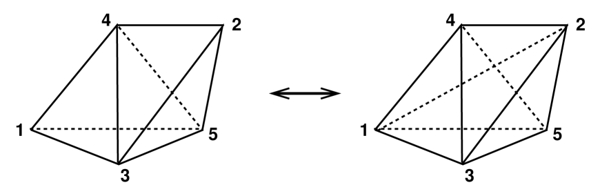
  Figure 5: The (2,3)-move in three dimensions.

7.2 Moves in four dimensions

If we distinguish between the space- and time-like character of all of the four-dimensional moves, there is a total of ten moves (including inverses). We will again characterize simplices in terms of their vertex labels. The first two types of moves, (2,8) and (4,6), reproduce a set of ergodic moves in three dimensions when restricted to spatial slices. We will describe each of the moves in turn.

• The initial configuration for this move is a pair of a (1,4)- and a (4,1)-simplex, sharing a purely space-like tetrahedron 3456 (Fig. 6).

  

  
  

  Figure 6: The (2,8)-move in four dimensions.

  The move consists in inserting an additional vertex 7 at the centre of this tetrahedron and subdiving the entire sub-complex so as to obtain eight four-simplices,

  $$1\underline{3456}+2\underline{3456}\rightarrow 1\underline{3457}+2\underline{3457}+1\underline{3467}+2\underline{3467}+1\underline{3567}+2\underline{3567}+1\underline{4567}+2\underline{4567},$$ (59)

  with an obvious inverse.

• In this configuration, we start from a pair (2345,3456) of spatial tetrahedra sharing a common triangle 345, which are connected to a vertex 1 at time $t\!-\!1$ and another vertex 7 at time $t\!+\!1$, forming together a sub-complex of size six (Fig. 7). The move consists in swapping the triangle 345 with its (spatially) dual edge 26, during which the two spatial tetrahedra are substituted by three, and the geometry above and below the spatial slice at time $t$ changed accordingly. In our by now familiar notation, this amounts to

  $$1\underline{2345}+\underline{2345}7+1\underline{3456}+\underline{3456}7\rightarrow 1\underline{2346}+\underline{2346}7+1\underline{2356}+\underline{2356}7+1\underline{2456}+\underline{2456}7,$$ (60)

  with the arrow reversed for the corresponding inverse move.

  

  
  

  Figure 7: The (4,6)-move in four dimensions.

• This type of move comes in two varieties. Its general structure is as follows: the initial configuration is a pair of 4-simplices with a common tetrahedron. During the move, this tetrahedron is “deleted” and substituted by its (in a four-dimensional sense) dual edge. The end result is a sub-complex consisting of four 4-simplices. From a Lorentzian point of view, there are two situations where the application of this move does not interfere with the slice-structure or the manifold constraints. In the first one, a (4,1)- and a (3,2)-tetrahedron from the same sandwich share a (3,1)-tetrahedron 3456 (Fig. 8). The dual edge 12 is time-like and shared in the final configuration by one (4,1)- and three (3,2)-simplices. The second possibility is that of two (3,2)-simplices sharing a (2,2)-tetrahedron. One of the (3,2)-simplices is “upside-down”, such that the entire sub-complex has spatial triangles in both the slices at $t$ and at $t\!+\!1$ (134 and 256, see Fig. 9). After the move, the total number of (3,2)-simplices has again increased by two. (Note that the changes of the bulk variables are encoded in the $f$-vectors of Sec. 8.) Both types of moves are described by the relation

  $$1\underline{3456}+2\underline{3456}\rightarrow\underline{12}345+\underline{12}346+\underline{12}456+\underline{12}356,$$ (61)

  and their inverses by the converse relation.

  

  
  

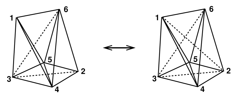
  Figure 8: The (2,4)-move in four dimensions, first version.

  

  
  

  Figure 9: The (2,4)-move in four dimensions, second version.

• The initial sub-complex in this type of move is made up of three 4-simplices which share a triangle in common. In the course of the move, this triangle is “deleted” and substituted by its dual (in a four-dimensional sense), which is again a triangle. It is straightforward to verify that this move can only occur in Lorentzian gravity if both of the triangles involved are time-like. Again, there are two allowed variations of the move. In the first one, both the initial and final sub-complex consist of one (4,1)- and two (3,2)-simplices, and the space-like edge of each of the triangles 123 and 456 lies in the same slice $t\!=\!const$ (Fig. 10). The 4-simplices are rearranged according to

  $$12\underline{456}+13\underline{456}+23\underline{456}\rightarrow\underline{123}45+\underline{123}46+\underline{123}56.$$ (62)

  

  
  

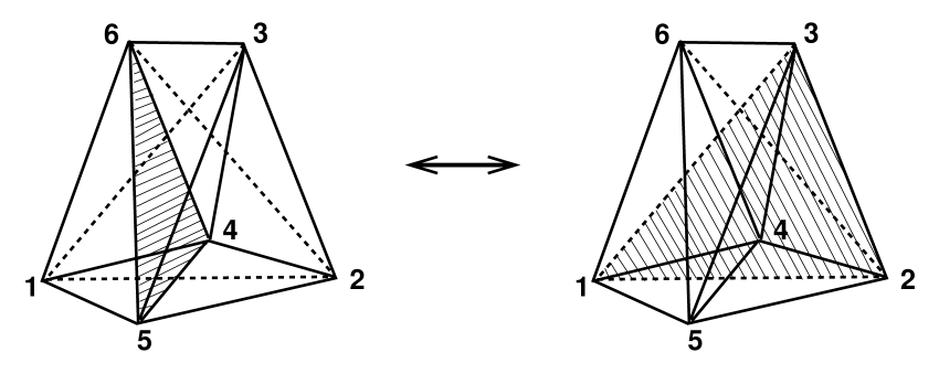
  Figure 10: The (3,3)-move in four dimensions, first version.

  

  
  

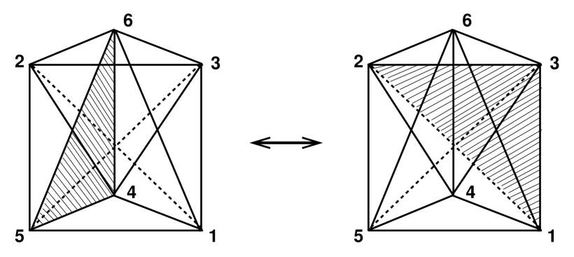
  Figure 11: The (3,3)-move in four dimensions, second version.

  The other initial configuration for which (62) can be performed involves only (3,2)-simplices of both orientations, as illustrated in Fig. 11. The “swapped” triangle 123 now has its space-like edge in the opposite spatial slice from that of the original triangle 456. As in the (4,4)-move in three dimensions, this type of move is its own inverse.

8 Kinematic bounds

Without solving the combinatorics of the Lorentzian gravity models explicitly, some qualitative insights can be gained by studying the behaviour of their partition functions for either very small or very large values of the inverse Newton’s constant $k$. By comparing our results with those of Euclidean dynamical triangulations in 3 and 4d [31, 32], we will see that significant differences arise already at this kinematic level. Since the partition function for Lorentzian gravity is evaluated after Wick-rotating, we will in the following set $\alpha\!=\!-1$, and work in the Euclidean sector of our models. We will perform the analysis for $d=3$ and $d=4$ in turn.

8.1 Analysis in three dimensions

For ease of comparison with the Euclidean results, we write the Regge action in standard form (c.f. (37)), namely, as

$$S_{\rm EDT}^{(3)}=k_{3}N_{3}-k_{1}N_{1},$$ (63)

with the couplings

$$k_{1}=2\pi k,\qquad k_{3}=6\ k\arccos\frac{1}{3}+\lambda\frac{1}{6\sqrt{2}}.$$ (64)

Lorentzian triangulations $T$ are conveniently characterized by their $f$-vectors $f(T)$, which keep track of the numbers (19) of simplicial building blocks. In three dimensions, we have

$$f^{(3)}=(N_{0},N_{1}^{\rm SL},N_{1}^{\rm TL},N_{2}^{\rm SL},N_{2}^{\rm TL},N_{3}^{(3,1)},N_{3}^{(2,2)}).$$ (65)

Rewriting the action as

$$S_{\rm EDT}^{(3)}=N_{3}(k_{3}-k_{1}\frac{N_{1}}{N_{3}})=:N_{3}(k_{3}-k_{1}\xi),$$ (66)

we see that for large coupling $k_{1}$ and at fixed space-time volume, configurations with a large value of $\xi$ will be energetically preferred. In the Euclidean case, it can be shown that in the thermodynamic limit $N_{3}\rightarrow\infty$, the ratio $\xi$ obeys the kinematic bounds

$$1\leq\xi\leq\frac{4}{3},\;\;\;\;\;\mbox{Euclidean 3d triangulations}.$$ (67)

The upper bound is saturated for so-called branched-polymer (or “stacked-sphere”) configurations. Geometrically degenerate configurations of this type dominate the partition function in the continuum limit and seem to be responsible for the failure of the Euclidean model to lead to an interesting continuum theory, both in three and four dimensions.

Obviously, the geometries of the Lorentzian model must satisfy (67), which is valid for all 3d simplicial manifolds. However, it turns out that the Lorentzian dynamical triangulations satisfy a more stringent upper bound. Using identities from Sec. 3, we can write

$$N_{3}=N_{3}^{(2,2)}+N_{3}^{(3,1)}=N_{3}^{(2,2)}+4N_{0}-4\chi t\geq N_{3,{\rm min}}^{(2,2)}+4N_{0}-4\chi t.$$ (68)

The minimal $N_{3}^{(2,2)}$ is given by $N_{3,{\rm min}}^{(2,2)}=c_{\rm min}t$, where $c_{\rm min}>0$ is an integer counting the minimal possible number of (2,2)-tetrahedra per time-step $\Delta t\!=\!1$. Using further identities, (68) therefore becomes

$$4N_{1}\leq 5N_{3}-(c_{\rm min}-4\chi)t.$$ (69)

From this we deduce that in the large-volume limit (where $t/N_{3}\rightarrow 0$) the upper bound for $\xi$ is lowered to $5/4$, so that the Euclidean relation (67) is substituted by

$$1\leq\xi\leq\frac{5}{4},\;\;\;\;\;\mbox{Lorentzian 3d triangulations}.$$ (70)

We conclude that the branched-polymer regime of Euclidean gravity cannot be realized in the Lorentzian case. The upper bound in (70) is saturated when the number of (2,2)-simplices is minimal.

There is an alternative way of deriving (70), which also sheds some light on the nature of the lower bound. Here, one asks whether the bounds on $\xi$ can be approached by a successive application of the Monte Carlo moves described in Sec. 7. In three dimensions, the effect of the Monte Carlo moves on the $f$-vector is

$$\Delta_{(2,6)}f^{(3)}=(1,3,2,2,6,4,0),$$ (71)

$$\Delta_{(4,4)}f^{(3)}=(0,0,0,0,0,0,0),$$ (72)

$$\Delta_{(2,3)}f^{(3)}=(0,0,1,0,2,0,1),$$ (73)

with obvious expressions for the inverse moves. Let us now choose some initial configuration $f_{0}^{(3)}$, for example, a $t$-translation-invariant geometry of minimal volume of the form $f_{0}^{(3)}=\vec{c}\ t$, where $\vec{c}$ is a constant seven-vector characterizing a sandwich geometry. Any triangulation that is reached from the initial one by a sequence of allowed Monte Carlo moves has an $f$-vector

$$f^{(3)}=(c_{1}t+x,c_{2}t+3x,c_{3}t+2x+y,c_{4}t+2x,c_{5}t+6x+2y,c_{6}t+4x,c_{7}t+y).$$ (74)

The integers $x=n_{(2,6)}-n_{(6,2)}$ and $y=n_{(2,3)}-n_{(3,2)}$ count the “excess” of applications of a move over its inverse. From (74) we can read off the value of $\xi$ as

$$\xi=\frac{N_{1}}{N_{3}}=\frac{(c_{2}+c_{3})t+5x+y}{(c_{6}+c_{7})t+4x+y}.$$ (75)

It is obvious that for large triangulations this ratio is maximized by applying only (2,6)-moves. This is always possible, since this Monte Carlo move is a subdivision move that can always be performed. In the infinite-volume limit (this also implies $x\gg t$), $\xi$ approaches $5/4$, in accordance with our earlier result. Alternatively, a triangulation can be enlarged by applying (2,3)-moves, which according to (73) increase the number of (2,2)-tetrahedra. It is not immediately clear that we can saturate the lower bound in (70) by taking $y\rightarrow\infty$ since $y$ is not entirely independent of $x$ (the applicability of the (2,3)-move is related to the availability of (3,1)-tetrahedra, which in turn is governed by $x$). Nevertheless, in the large-volume limit such configurations do actually exist, as we will demonstrate below.

Another type of degenerate geometry that was observed to dominate the state sums of Euclidean dynamical triangulations at small $k$ [33, 34] is characterized by an inequality which is non-linear in the bulk variables, namely,

$$N_{1}\leq\frac{1}{2}N_{0}(N_{0}-1).$$ (76)

A triangulation saturating (76) is called “2-neighbourly” [32] since any of its vertices is connected by an edge to any other vertex. The resulting space is of maximal Hausdorff dimension, because “one can get anywhere in a single step”. Such singular structures have indeed been observed in the so-called crumpled phase of Euclidean quantum gravity in three and four dimensions.

Again, it is impossible to come anywhere near this phase in the continuum limit of the Lorentzian model. This has to do with the fact that by construction of the Lorentzian geometries, two vertices can only be connected by a link if they lie in the same or in successive spatial slices. Instead of (76), we therefore have separate relations for the numbers $N_{1}^{{\rm SL}}$ and $N_{1}^{{\rm TL}}$ of space- and time-like edges,

$$N_{1}^{\rm SL}=\sum_{\tau=0}^{t-1}(3N_{0}(\tau)-6)=3N_{0}-6t,\qquad N_{1}^{\rm TL}\leq\sum_{\tau=0}^{t-1}N_{0}(\tau)N_{0}(\tau+1).$$ (77)

Assuming canonical scaling, the right-hand side of the inequality (76) behaves like (length)⁶, whereas the second relation in (77) scales only like (length)⁵, proving our earlier statement.

Figure 12: One of a sequence of toroidal sandwich configurations at $\tau+1/2$ which saturate the inequality in (77) in the large-volume limit (opposite sides to be identified). Light links correspond to triangle edges at time $\tau$, dark links to triangle edges at time $\tau+1$.

The inequality in (77) can indeed be saturated by certain regular Lorentzian geometries in the large-volume limit, as one can show by explicit construction. For ease of visualization, let us assume that the two-dimensional slices have the topology of two-tori $T^{2}$. Consider a sandwich where the initial two-geometry at time $\tau$ is a “strip” of discrete length $l_{1}$ and width $c_{1}=2$, consisting of $2l_{1}+4$ triangles, with opposite sides identified to give a torus. Similarly, at time $\tau+1$, take a strip of length $l_{2}$ and width $c_{2}=2$ with $2l_{2}+4$ triangles. Choose the interpolating geometry between the two tori such that the (2,2)-tetrahedra when viewed at time $\tau+1/2$ form two rectangular blocks, of size $l_{1}l_{2}$ and of size $c_{1}c_{2}$ (Fig. 12). Consider now a sequence of such configurations where both of the $l_{i}$ become large, but the integers $c_{i}$ remain unchanged. Because of $N_{0}(\tau)=N_{1}^{\rm SL}(\tau)/3=l_{1}+2$ and $N_{0}(\tau+1)=N_{1}^{\rm SL}(\tau+1)/3=l_{2}+2$, we find that in the large-volume limit the bulk variables associated with the sandwich are given by $N_{1}\approx N_{1}^{\rm TL}\approx l_{1}l_{2}$, and by $N_{3}=N_{2}^{\rm SL}(\tau)+N_{2}^{\rm SL}(\tau+1)+N_{3}^{(2,2)}\approx l_{1}l_{2}$. For the vertex numbers, we have $N_{0}(\tau)N_{0}(\tau+1)\approx l_{1}l_{2}$. This verifies our earlier claims that both the inequality (77) and the lower bound in (70) are saturated by this class of configurations. Of course, we achieved this by a “fine-tuning” of geometry, and the configurations thus obtained are highly non-generic.

The above considerations show that the phase structure of three-dimensional Lorentzian gravity must be quite different from that of the Euclidean theory since already at a kinematic level, the extreme branched-polymer and crumpled configurations cannot be realized. Obviously it does not exclude the possibility that milder pathologies prevail in the continuum limit, but it is clearly a step in the right direction. Hopes that the Lorentzian model is therefore better-behaved than its Euclidean counterpart have been boosted by recent numerical investigations in three dimensions [16, 30]. There it was found that for a large range of the gravitational coupling constant $k_{1}$, the partition function is dominated by a phase of extended geometry (and the parameter $\xi$ stays well away from its extremal bounds (70)), whose global scaling properties are those of a three-dimensional object. Compared with the Euclidean case, this is a completely new and very promising phenomenon. It reiterates the finding in $d=2$ [7] that the causal structure of the Lorentzian space-times acts effectively as a regulator for the quantum geometry.

8.2 Analysis in four dimensions

The analysis of the kinematic bounds in four dimensions is completely analogous to that of the previous subsection, and we will refrain from spelling out all the details. We start from the action in the form (c.f. (42))

$$S_{\rm EDT}^{(4)}=k_{4}N_{4}-k_{2}N_{2}=N_{4}(k_{4}-k_{2}\frac{N_{2}}{N_{4}})=:N_{4}(k_{4}-k_{2}\xi^{\prime}),$$ (78)

with the coupling constants

$$k_{2}=\frac{\sqrt{3}}{2}\pi k,\qquad k_{4}=\frac{5\sqrt{3}}{2}k\arccos\frac{1}{4}+\lambda\frac{\sqrt{5}}{96}.$$ (79)

In (78) we have already anticipated that a convenient order parameter in four dimensions is the quotient $\xi^{\prime}=N_{2}/N_{4}$. The $f$-vector has now length 10, and is given by

$$f^{(4)}=(N_{0},N_{1}^{\rm SL},N_{1}^{\rm TL},N_{2}^{\rm SL},N_{2}^{\rm TL},N_{3}^{\rm SL},N_{3}^{(3,1)},N_{3}^{(2,2)},N_{4}^{(4,1)},N_{4}^{(3,2)}).$$ (80)

The discussion parallels closely the three-dimensional case, with the relevant Euclidean inequalities [31, 32]

$$2\leq\xi^{\prime}\leq\frac{5}{2},\;\;\;\;\;\mbox{Euclidean 4d triangulations}.$$ (81)

Let us derive their Lorentzian analogues by analyzing the effect of the Monte Carlo moves of Sec. 7 on the $f$-vector (80), which is

$$\Delta_{(2,8)}f^{(4)}=(1,4,2,6,8,3,12,0,6,0),$$ (82)

$$\Delta_{(4,6)}f^{(4)}=(0,1,0,2,2,1,4,0,2,0),$$ (83)

$$\Delta_{(2,4)}f^{(4)}=(0,0,1,0,4,0,2,3,0,2),$$ (84)

$$\Delta_{(3,3)}f^{(4)}=(0,0,0,0,0,0,0,0,0,0).$$ (85)

Starting from a minimal initial configuration $f_{0}^{(4)}$, and defining $x=n_{(2,8)}-n_{(8,2)}$, $y=n_{(4,6)}-n_{(6,4)}$ and $z=n_{(2,4)}-n_{(4,2)}$, and dropping terms proportional to $t$ in the large-volume limit, one obtains

$$\xi^{\prime}=\frac{N_{2}}{N_{4}}\longrightarrow\frac{7x+2(y+z)}{3x+y+z}.$$ (86)

Again, $\xi^{\prime}$ is maximized by applying the subdivision move (2,8) only. Note also that – like in three dimensions – this corresponds to creating stacked-sphere configurations within the spatial slices of constant integer-$t$. (We are using the expression “stacked spheres” in a loose sense, and only require that the triangulations look like stacked spheres almost everywhere.) For the purposes of relation (86), the moves (4,6) and (2,4) play an equivalent role, although they generate different types of four-simplices. It is clear that a lower bound for the ratio is given by 2, although again it is not immediately clear that this value can actually be attained by any triangulation in the thermodynamic limit. Like in 3d, we can conclude that the range for the parameter $\xi^{\prime}$ in Lorentzian gravity is reduced, such that

$$2\leq\xi^{\prime}\leq\frac{7}{3},\;\;\;\;\;\mbox{Lorentzian 4d triangulations}.$$ (87)

We leave it as an exercise to the reader to prove this relation directly from (67) and the identities in Sec. 3, as well as to construct explicit triangulations that saturate the lower bound. Again, our analysis implies the absence of the polymeric geometries found in the Euclidean theory. (Note that a polymeric behaviour is in principle allowed both in three- and four-dimensional Lorentzian triangulations, as long as it takes place in the spatial directions only. In fact, this corresponds precisely to the limit $x\rightarrow\infty$ in both (75) and (86).) Likewise, there is no crumpled phase. The argument of $d=3$ carries over to four dimensions, with the only difference that the right-hand side of (76) scales like (length)⁸, whereas the corresponding relation in (77) scales like (length)⁷.

9 Summary and outlook

In this paper, we have presented a comprehensive analysis of a regularized path integral for gravity in terms of Lorentzian dynamical triangulations. We have shown that for a finite space-time volume $N$ the model is well-defined as a statistical system of geometry, with a finite state sum.

Having established these properties, our main interest is the behaviour of the system in a suitable continuum limit. For this, we must take the lattice volume $N\rightarrow\infty$ and the invariant lattice spacing $a\rightarrow 0$, and allow for a renormalization of both the bare coupling constants and the propagator itself. Although the discretized set-up of our model looks rather similar in different dimensions, we expect the details of the renormalization and the resulting physics to depend strongly on $d$.

The continuum theory in $d=2$ is already explicitly known, since the Lorentzian model has been solved exactly [7, 8]. It is obtained by simply taking $N\rightarrow\infty$ or, equivalently, tuning the bare cosmological constant $\lambda$ to its critical value. The theory describes a one-dimensional spatial “quantum universe” whose volume fluctuates in time. Obviously the physical significance of this model is somewhat obscure, since there is no classical theory of 2d Einstein gravity, and therefore no well-defined classical limit. Nevertheless, it provides a beautiful example of the inequivalence of path integrals of Euclidean and Lorentzian geometries. What is more, we understand in a very explicit manner [7, 35] that the origin of the difference lies in the presence and absence of “baby universes” branching off in the time-direction (which in the Lorentzian case are incompatible with the “micro-causality” of the path-integral histories).

“Solving the path integral” in our formulation amounts to solving the combinatorics of the Lorentzian triangulations in a given dimension and for given boundary data, at least asymptotically. Although this counting problem is mathematically well-defined, it is not simple when $d\geq 3$. In three space-time dimensions, where the problem is presently under investigation, an interesting relation with an already known matrix model with ABAB-interaction has been uncovered [19].

A potentially powerful feature of our models is the fact that they can also be studied numerically. Using Monte Carlo methods, it was shown that 2d Lorentzian gravity coupled to matter has no barrier at $c=1$ [36], and that pure 3d Lorentzian gravity possesses a ground state of extended geometry, with the global scaling properties of a three-dimensional space-time universe [16, 30]. Both of these findings are highly significant, because they show that these models lie in different universality classes from their Euclidean counterparts.

Let us recapitulate how this difference with the purely Euclidean formulation came about. Our physical premise was to take the space of Lorentzian space-times as our starting point. This enabled us to impose certain causality constraints on the individual histories contributing to the path integral. As a consequence, like in classical relativity, “time”- and “space”-directions are not interchangeable, a feature that persists in the continuum quantum theory. In order for this philosophy to lead anywhere (i.e. to yield convergent mathematical expressions) we crucially needed a Wick rotation on the space of Lorentzian geometries. The fact that such a map exists in our formulation is by no means trivial. For example, if a similar construction were attempted in Regge calculus, one would immediately run into trouble with triangular inequalities.

Being familiar with the pitfalls of Euclidean gravitational path integrals, one may now wonder whether our path integrals after the Wick rotation to Euclidean signature do not also suffer from pathologies, in the limit as $N\rightarrow\infty$. In particular, one may worry about the presence of a conformal divergence in $d\geq 3$ associated with the unboundedness of the gravitational action. Remarkably, although such a divergence is potentially present in our formulation, since configurations with large negative action exist, these are entropically suppressed in the continuum limit, at least in $d=3$ [16]. It has been demonstrated in [37] how this phenomenon can be understood from the point of view of the continuum gravitational path integral: a careful analysis of various Faddeev-Popov determinants reveals how the resulting path-integral measure can lead to a non-perturbative cancellation of the conformal divergence.

To summarize, we have constructed a new and powerful calculational tool for quantum gravity that in the best of all worlds will lead to a non-perturbative definition of an interacting quantum theory of gravity in four dimensions. An inclusion of other matter degrees of freedom is in principle straightforward. At the discretized level, our models are as well-defined as one could hope for. An investigation in dimension 3, both analytically and numerically, is well under way. It remains a major challenge to set up sufficiently large numerical simulations in four dimensions. Clearly, because of the anisotropy between time and spatial directions, larger lattice sizes than in the Euclidean dynamically triangulated models will be needed. On the analytic front, tackling the full combinatorics in four dimensions will be difficult, as one would expect from any fully-fledged formulation of quantum gravity. In order to approach the problem, we are currently studying both the three-dimensional theory and its relation to other formulations of 3d quantum gravity, as well as gravitational models with extra symmetries.

Acknowledgements

All authors acknowledge support by the EU network on “Discrete Random Geometry”, grant HPRN-CT-1999-00161, and by ESF network no.82 on “Geometry and Disorder”. In addition, J.A. and J.J. were supported by “MaPhySto”, the Center of Mathematical Physics and Stochastics, financed by the National Danish Research Foundation, and J.J. by KBN grants 2P03B 019 17 and 998 14.

Appendix 1: Lorentzian angles

For the sake of completeness, we will describe some properties of Lorentzian angles (or “boosts”) which appear in the Regge scalar curvature as rotations about space-like bones (that is, space-like links in 3d and space-like triangles in 4d). This summarizes the treatment and conventions of [21]. The familiar form of a contribution of a single bone $b$ to the total curvature and therefore the action is

$$\Delta_{b}S={\rm volume}(b)\delta_{b},\;\;\;\;\delta_{b}=2\pi-\sum_{i}\Theta_{bi},$$ (88)

where the volume of the bone is by definition real and positive and $\delta_{b}$ is the deficit angle around $b$. For the case of Euclidean angles this is conveniently illustrated by a two-dimensional example, where the bone is simply a point with volume 1. A positive deficit angle $\delta$ (Fig. 13a) implies a positive Gaussian curvature and therefore a positive contribution to the action, whereas an “excess” angle $\delta$ contributes negatively (Fig. 13b).

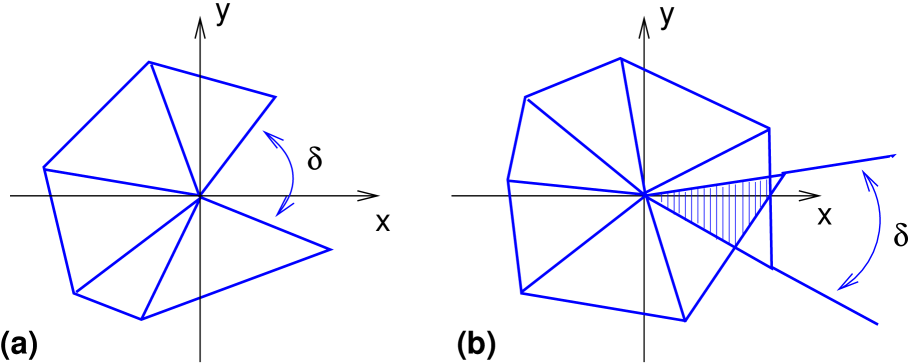
Figure 13: Positive (a) and negative (b) Euclidean deficit angles $\delta$.

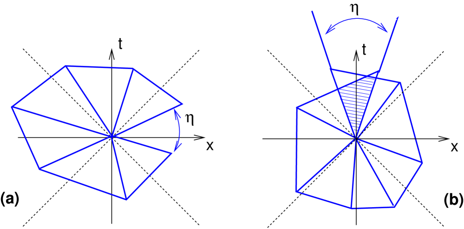
Figure 14: Positive space-like (a) and time-like (b) Lorentzian deficit angles $\eta$.

Lorentzian angles are also defined to be additive, in such a way that a complete rotation around a space-like bone gives $2\pi$ in the flat case. However, note that the angles are in general complex, and can become arbitrarily large in the vicinity of the light cone. In their contribution to the action, we have to distinguish between two cases. If the Lorentzian deficit angle $\delta\equiv\eta$ is space-like (Fig. 14a), it contributes as $\Delta_{b}S={\rm volume}(b)\eta_{b}$, just like in the Euclidean case. By contrast, if it is time-like (Fig. 14b), the deficit angle contributes with the opposite sign, that is, as $\Delta_{b}S=-{\rm volume}(b)\eta_{b}$. Therefore, both a space-like defect and a time-like excess increase the action, where as a time-like defect or a space-like excess decrease it.

The deficit angles in Sections 2.1 and 2.2 were calculated using

$$\cos\Theta=\frac{\langle\vec{v}_{1},\vec{v}_{2}\rangle}{\langle\vec{v}_{1},\vec{v}_{1}\rangle^{\frac{1}{2}}\langle\vec{v}_{2},\vec{v}_{2}\rangle^{\frac{1}{2}}},\;\;\;\;\sin\Theta=\frac{\sqrt{\langle\vec{v}_{1},\vec{v}_{1}\rangle\langle\vec{v}_{2},\vec{v}_{2}\rangle-\langle\vec{v}_{1},\vec{v}_{2}\rangle^{2}}}{\langle\vec{v}_{1},\vec{v}_{1}\rangle^{\frac{1}{2}}\langle\vec{v}_{2},\vec{v}_{2}\rangle^{\frac{1}{2}}},$$ (89)

for pairs of vectors $\vec{v}_{1},\vec{v}_{2}$, and the flat Minkowskian scalar product $\langle\cdot,\cdot\rangle$. By definition, the square roots are positive imaginary for negative arguments.

Appendix 2: Link-reflection positivity in 2d

In this appendix we will demonstrate the link-reflection positivity of the discrete model of two-dimensional Lorentzian quantum gravity introduced in [7]. Recall that link reflection is the reflection at a plane of half-integer $t$. We choose it to lie at $t=1/2$ and fix the boundary spatial lengths at the initial time $t=-T+1$ and the final time $t=T$ to $l_{-T+1}=l_{T}=l$. In order to describe a two-dimensional Lorentzian universe with these boundary conditions, we must not only specify the geometry of the spatial sections (simply given by $l_{t}$, $-T+1\leq t\leq T$), but the connectivity of the entire 2d triangulation.

A convenient way of parametrizing the connectivity that is symmetric with respect to incoming and outgoing triangles at any given slice of constant $t$ is as follows. For any spatial slice at some integer time $t$, each of the $l_{t}$ spatial edges forms the base of one incoming and one outgoing triangle. The geometry of the adjoining sandwiches is determined by how these triangles are glued together pairwise along their time-like edges. These gluing patterns correspond to distinct ordered partitions of the $l_{t}$ triangles (either above or below $t$) into $k$ groups, $1\leq k\leq l_{t}$. We denote the partitions collectively by $m(t)=\{m_{r}(t),\ r=1,\ldots,k\}$ for the incoming triangles and by $n(t)=\{n_{r}(t),\ r=1,\ldots,k^{\prime}\}$ for the outgoing triangles. The constraints on these variables are obviously $\sum_{r=1}^{k}m_{r}(t)=\sum_{r=1}^{k^{\prime}}n_{r}(t)=l_{t}$ and a matching condition for adjacent slices, namely, $k^{\prime}(t)=k(t+1)$. In terms of these variables, the (unmarked) one-step propagator is given by

$$G_{g}(l_{1},l_{2})=g^{l_{1}+l_{2}}\sum_{k\geq 1}\;\frac{1}{k}\ \sum_{{n_{r},m_{r}\geq 1,\ r=1,\ldots,k\atop\sum_{q=1}^{k}n_{q}=l_{1},\ \sum_{p=1}^{k}m_{p}=l_{2}}}1\;=g^{l_{1}+l_{2}}\sum_{k\geq 1}\;\frac{1}{k}\ {l_{1}-1\choose l_{1}-k}{l_{2}-1\choose l_{2}-k},$$ (90)

where $g={\rm e}^{-\lambda}$ depends on the two-dimensional cosmological constant $\lambda$. It is obvious from (90) that the propagator depends symmetrically on the local variables $m$ and $n$. The partition function for the entire system is

$$Z_{2d}(g)=G_{g}(l_{-T+1},l_{-T+2})\prod_{t=-T+2}^{T-1}\,\sum_{l_{t}\geq 1}l_{t}\ G_{g}(l_{t},l_{t+1}),$$ (91)

in accordance with (47).

Following the discussion of link reflection in Sec. 6, we consider now functions $F(\{m,n\})$ that depend only on the geometry above the reflecting plane at $t=1/2$, i.e. on $m(t)$, $n(t)$, $t\geq 1$. The reflection (52) acts on the partition data according to $\theta_{l}(m(t))=n(-t+1)$ and $\theta_{l}(n(t))=m(-t+1)$. Without loss of generality, we can assume that $F$ depends symmetrically on $m(t)$ and $n(t)$, $\forall t$. Computing the expectation value (54), we obtain

$$\langle(\theta_{l}F)F\rangle$$

$$\hskip 8.5359pt=Z_{2d}^{-1}\sum_{l_{0},l_{1}\geq 1}l_{0}l_{1}G_{g}(l_{0},l_{1})\Bigl{(}G_{g}(l_{-T+1},l_{-T+2})\prod_{t=-T+2}^{-1}\sum_{l_{t}\geq 1}l_{t}G_{g}(l_{t},l_{t+1})(\theta_{l}F)\Bigr{)}\times$$

$$\hskip 39.83368pt\Bigl{(}\prod_{t=1}^{T-2}\sum_{l_{t+1}\geq 1}G_{g}(l_{t},l_{t+1})l_{t+1}G_{g}(l_{T-1},l_{T})F\Bigr{)}$$

$$\hskip 8.5359pt=Z_{2d}^{-1}\sum_{l_{0},l_{1}\geq 1}l_{0}l_{1}\sum_{k\geq 1}\ \frac{1}{k}\ g^{l_{0}+l_{1}}{l_{0}-1\choose l_{0}-k}{l_{1}-1\choose l_{1}-k}\ \overline{{\bf F}(l_{0})}{\bf F}(l_{1})$$

$$\hskip 8.5359pt=Z_{2d}^{-1}\sum_{k\geq 1}\ \frac{1}{k}\ \overline{{\cal F}(k)}{\cal F}(k).$$ (92)

Since the last expression is a sum of positive terms, we have hereby shown that 2d Lorentzian gravity is link-reflection positive.

References

- [1] P. Ginsparg and G. Moore: Lectures on 2D gravity and 2D string theory, in: Recent directions in particle theory: from superstrings and black holes to the standard model (TASI-92), eds. J. Harvey and J. Polchinski (World Scientific, Singapore, 1993) 277-470 [hep-th/9304011].
- [2] F. David: Simplicial quantum gravity and random lattices, in: Gravitation and quantizations (Les Houches Summer School, Session LVII, 1992), eds. J. Zinn-Justin and B. Julia (Elsevier, Amsterdam, 1995) 679-750 [hep-th/9303127].
- [3] R.M. Williams: Recent progress in Regge calculus, Nucl. Phys. B (Proc. Suppl.) 57 (1997) 73-81 [gr-qc/9702006].
- [4] J. Ambjørn: Quantum gravity represented as dynamical triangulations, Class. Quant. Grav. 12 (1995) 2079-2134.
- [5] J. Ambjørn, J. Jurkiewicz and R. Loll: Lorentzian and Euclidean quantum gravity – analytical and numerical results, in: M-Theory and Quantum Geometry, eds. L. Thorlacius and T. Jonsson, NATO Science Series (Kluwer Academic Publishers, 2000) 382-449 [hep-th/0001124].
- [6] R. Loll: Discrete approaches to quantum gravity in four dimensions, Living Reviews in Relativity 13 (1998), http://www.livingreviews.org [gr-qc/9805049].
- [7] J. Ambjørn and R. Loll: Non-perturbative Lorentzian quantum gravity, causality and topology change, Nucl. Phys. B 536 (1998) 407-434 [hep-th/9805108].
- [8] J. Ambjørn, R. Loll, J.L. Nielsen and J. Rolf: Euclidean and Lorentzian quantum gravity – lessons from two dimensions, J. Chaos Solitons Fractals 10 (1999) 177-195 [hep-th/9806241].
- [9] R. Loll: Discrete Lorentzian quantum gravity, Nucl. Phys. B (Proc. Suppl.) 94 (2001) 96-107 [hep-th/0011194].
- [10] A. Krzywicki: Random manifolds and quantum gravity, Nucl. Phys. B (Proc. Suppl.) 83 (2000) 126-130 [hep-lat/9907012]; G. Thorleifsson: Lattice gravity and random surfaces, Nucl. Phys. B (Proc. Suppl.) 73 (1999) 133-145 [hep-lat/9809131]; M. Bowick: Random surfaces and lattice gravity, Nucl. Phys. B (Proc. Suppl.) 63 (1998) 77-88 [hep-lat/9710005]; D.A. Johnston: Gravity and random surfaces on the lattice: a review, Nucl. Phys. B (Proc. Suppl.) 53 (1997) 43-55 [hep-lat/9607021].
- [11] S. Caracciolo and A. Pelissetto: Phases and topological structures of de Sitter lattice gravity, Nucl. Phys. B 299 (1988) 693-718.
- [12] W. Beirl, E. Gerstenmayer, H. Markum and J. Riedler: The well defined phase of simplicial quantum gravity in four-dimensions, Phys. Rev. D 49 (1994) 5231-5239 [hep-lat/9402002]; W. Beirl, A. Hauke, P. Homolka, H. Markum and J. Riedler: Correlation functions in lattice formulation of quantum gravity, Nucl. Phys. B (Proc. Suppl.) 53 (1997) 735-738 [hep-lat/9608055].
- [13] P. Bialas, Z. Burda, A. Krzywicki and B. Petersson: Focusing on the fixed point of 4-d simplicial gravity, Nucl. Phys. B 472 (1996) 293-308 [hep-lat/9601024]; B.V. de Bakker: Further evidence that the transition of 4-d dynamical triangulation is first order, Phys. Lett. B 389 (1996) 238-242 [hep-lat/9603024].
- [14] H.W. Hamber: On the gravitational scaling dimensions, Phys. Rev. D 61 (2000) 124008 [hep-th/9912246].
- [15] J. Ambjørn, J. Jurkiewicz and R. Loll: Nonperturbative Lorentzian path integral for gravity, Phys. Rev. Lett. 85 (2000) 924-927 [hep-th/0002050].
- [16] J. Ambjørn, J. Jurkiewicz and R. Loll: Non-perturbative 3d Lorentzian quantum gravity, Phys. Rev. D, to appear [hep-th/0011276].
- [17] J. Ambjørn, J. Jurkiewicz and Y.M. Makeenko: Multiloop correlators for two-dimensional quantum gravity, Phys. Lett. B 251 (1990) 517-524.
- [18] P. Di Francesco, E. Guitter and C. Kristjansen: Integrable 2d Lorentzian gravity and random walks, Nucl. Phys. B 567 (2000) 515-553 [hep-th/9907084].
- [19] J. Ambjørn, J. Jurkiewicz, R. Loll and G. Vernizzi: Lorentzian 3d gravity with wormholes via matrix models, preprint AEI-Golm, to appear.
- [20] J.A. Wheeler: Geometrodynamics and the issue of the final state, in Relativity, groups and topology, eds. B. DeWitt and C. DeWitt (Gordon and Breach, New York, 1964); J.B. Hartle: Simplicial minisuperspace I. General discussion, J. Math. Phys. 26 (1985) 804-814.
- [21] R. Sorkin: Time-evolution in Regge calculus, Phys. Rev. D 12 (1975) 385-396; Err. ibid. 23 (1981) 565.
- [22] J. Ambjørn and J. Jurkiewicz: Four-dimensional simplicial quantum gravity, Phys. Lett. B 278 (1992) 42-50.
- [23] J. Ambjørn, M. Carfora and A. Marzuoli: The geometry of dynamical triangulations, Lecture Notes in Physics, New Series, m50 (Springer, Berlin, 1997) [hep-th/9612069].
- [24] J. Ambjørn and S. Varsted: Three-dimensional simplicial quantum gravity, Nucl. Phys. B 373 (1992) 557-580.
- [25] R. Nakayama: 2-d quantum gravity in the proper time gauge, Phys. Lett. B 325 (1994) 347-353 [hep-th/9312158].
- [26] K. Osterwalder and R. Schrader: Axioms for Euclidean Green’s functions I& II, Commun. Math. Phys. 31 (1973) 83-112, 42 (1975) 281-305; E. Seiler: Gauge theories as a problem of constructive quantum field theory and statistical mechanics, Lecture Notes in Physics 159 (Springer, Berlin, 1982).
- [27] J. Glimm and A. Jaffe: Quantum physics, Second edition (Springer, New York, 1987).
- [28] I. Montvay and G. Münster: Quantum fields on a lattice (Cambridge University Press, Cambridge, UK, 1994).
- [29] M. Gross and S. Varsted: Elementary moves and ergodicity in d-dimensional simplicial quantum gravity, Nucl. Phys. B 378 (1992) 367-380.
- [30] J. Ambjørn, J. Jurkiewicz and R. Loll: Computer simulations of 3d Lorentzian quantum gravity, Nuclear Physics B (Proc. Suppl.) 94 (2001) 689-692 [hep-lat/ 0011055].
- [31] D. Gabrielli: Polymeric phase of simplicial quantum gravity, Phys. Lett. B 421 (1998) 79-85 [hep-lat/9710055].
- [32] J. Ambjørn, M. Carfora, D. Gabrielli and A. Marzuoli: Crumpled triangulations and critical points in 4D simplicial quantum gravity, Nucl. Phys. B 542 (1999) 349-394 [hep-lat/9806035].
- [33] T. Hotta, T. Izubuchi and J. Nishimura: Singular vertices in the strong coupling phase of four-dimensional simplicial gravity, Prog. Theor. Phys. 94 (1995) 263-270 [hep-lat/9709073]; Nucl. Phys. B (Proc. Suppl.) 47 (1996) 609-612 [hep-lat/9511023].
- [34] S. Catterall, G. Thorleifsson, J. Kogut and R. Renken: Singular vertices and the triangulation space of the d sphere, Nucl. Phys. B 468 (1996) 263-276 [hep-lat/9512012]; S. Catterall, J. Kogut and R. Renken: Singular structure in 4-d simplicial gravity, Phys. Lett. B 416 (1998) 274-280 [hep-lat/9709007].
- [35] J. Ambjørn, J. Correia, C. Kristjansen and R. Loll: The relation between Euclidean and Lorentzian 2D quantum gravity, Phys. Lett. B 475 (2000) 24-32 [hep-th/9912267].
- [36] J. Ambjørn, K.N. Anagnostopoulos and R. Loll: A new perspective on matter coupling in 2d quantum gravity, Phys. Rev. D 60 (1999) 104035 [hep-th/9904012]; Crossing the c1 barrier in 2d Lorentzian quantum gravity, Phys. Rev. D 61 (2000) 044010 [hep-lat/9909129].
- [37] A. Dasgupta and R. Loll: A proper-time cure for the conformal sickness in quantum gravity, Nucl. Phys. B, to appear [hep-th/0103186].