DAMTP-2001-108

hep-th/0112077

Intersoliton forces in the Wess-Zumino model
 Ruben Portugues and  Paul K. Townsend

DAMTP, University of Cambridge,
Centre for Mathematical Sciences, Wilberforce Road,
Cambridge CB3 0WA, UK

ABSTRACT

The spectrum of supersymmetric domain wall solitons of the Wess-Zumino model is known to be discontinuous across a curve (of marginal stability) in the moduli space of quartic superpotentials. Here we show how this phenomenon can be understood from the behaviour of the long-range inter-soliton force, which we compute by a method due to Manton.

1 Introduction

It is often stated that solitons of supersymmetric field theories that preserve the same fraction of supersymmetry will exert no force on each other. When true, this implies the existence of static supersymmetric multi-soliton solutions that can be interpreted as individual solitons in static marginal equilibrium due to a cancellation of attractive and repulsive forces. However, static supersymmetric multi-soliton solutions may not exist. This is typically the case for domain walls; i.e. solitons of (1+1)-dimensional field theories. Although it is possible to find (1+1)-dimensional models that admit multi-soliton solutions of the type described above [1], these seem to be the exception rather than the rule. In general, multi-soliton solutions of (1+1)-dimensional field theories are time-dependent, and this implies the existence of a force between the constituent solitons.

Consider the case of a field theory for a real scalar field $\phi$ with a potential having three isolated degenerate minima, at $\phi_{a}<\phi_{b}<\phi_{c}$. There exist static soliton solutions interpolating between the adjacent minima, and these are supersymmetric solutions of the supersymmetric version of this model, but there is no supersymmetric soliton interpolating between the non-adjacent minima. This is because all supersymmetric solutions correspond to flows of a first-order equation and there is no flow connecting $\phi_{a}$ with $\phi_{c}$. There must be some solutions that interpolate between the non-adjacent minima, but they are necessarily time-dependent. These solutions represent an $ab$-soliton followed by a $bc$-soliton moving under the influence of the force between them, at least for large separation. The leading-order term in an asymptotic expansion of the long-range force must be repulsive because an attractive force would imply the existence of a bound state of an $ab$-soliton with a $bc$-soliton and hence the existence of an $ac$-soliton but, as we have just explained, there is no such soliton. We shall confirm the repulsive nature of the long-range force, as a special case of a more general result, by adapting a method introduced by Manton [2] to compute the long-range attractive force between a soliton and its anti-soliton.

The situation for multi-component scalar field theories is much more complicated. Here we concentrate on domain walls of the bosonic sector of the Wess-Zumino model for a single complex scalar superfield. On reduction to (1+1) dimensions this becomes a model for a single complex scalar field $z(t,s)$ with Lagrangian density

$${\cal L}={1\over 2}\left[|\dot{z}|^{2}-|z^{\prime}|^{2}-|\partial W(z)|^{2}\right]\,,$$ (1)

where the ‘superpotential’ $W(z)$ is a holomorphic function, and

$$\dot{z}\equiv{\partial z\over\partial t}\,,\qquad z^{\prime}\equiv{\partial z\over\partial s}\,,\qquad\partial W={\partial W\over\partial z}\,.$$ (2)

Critical points of $W$ are degenerate global minima of the potential and solitons are minimal energy configurations that interpolate between them. In the supersymmetric context, the critical points of $W$ are supersymmetric vacua and the solitons interpolating between them preserve 1/2 of the supersymmetry [3, 4, 5].

Polynomials provide a simple class of superpotentials. A polynomial superpotential of order $n$ has $n-1$ critical points, and hence $n-1$ vacua, so in order for such a model to admit multi-soliton configurations we need $n\geq 4$. Here we shall concentrate on the simplest case of a quartic superpotential, which may (without loss of generality) be put in the form

$$W(z)=z^{4}-\frac{4}{3}\mu z^{3}-2z^{2}+4\mu z\,,$$ (3)

where $\mu$ is a complex constant that parametrizes the space of physically-distinct quartic superpotentials [4]. Provided that $\mu\neq\pm 1$, there are then three (degenerate) supersymmetric vacua, at

$$(1):\ z=-1,\qquad(2):\ z=1,\qquad(3):\ z=\mu\ ,$$ (4)

and hence, potentially, three soliton solutions interpolating between them. However, whether all three types of soliton actually exist depends on the value of $\mu$. For example, if $\mu=0$ then soliton solutions $z(s)$ are real (because all three vacua lie on the real axis in the $z$-plane) and can connect only adjacent vacua; there are therefore only two types of soliton. On the other hand, the choice

$$\mu=i\sqrt{3}$$ (5)

yields a $Z_{3}$-symmetric model for which the existence of all three solitons is guaranteed by symmetry given any one of them.

The $\mu$-dependence of the soliton spectrum of the WZ model with superpotential (3) was analysed in [4], where it was shown that the ‘2-soliton’ to ‘3-soliton’ frontiers in the $\mu$-plane are the two branches of a curve $\Delta(\mu_{1},\mu_{2})=0$, where we have set $\mu=\mu_{1}+i\mu_{2}$ and

$$\Delta\equiv 3-6\mu_{1}^{2}-6\mu_{2}^{2}-\mu_{2}^{4}+2\mu_{1}^{2}\mu_{2}^{2}+3\mu_{1}^{4}\,.$$ (6)

This curve is shown in Fig. 1; when it is crossed from inside a ‘3-soliton’ region, one of the three solitons disappears from the spectrum.

Figure 1: The curve of marginal stability separating the ‘2-soliton’ and ‘3-soliton’ regions in the $\mu$-plane, where $\mu=\mu_{1}+i\mu_{2}$.

The curve $\Delta=0$ is therefore a simple (and, apparently, the earliest) example of what is now called a curve of marginal stability. The reason for the discontinuity in the soliton spectrum across this curve was explained in [4]: consider what happens as we start from the $\hbox{\mybb Z}_{3}$-symmetric case (5) and proceed down the imaginary $\mu$ axis to the origin. As $\mu_{2}$ decreases, the soliton trajectory in the $z$-plane that starts at vacuum 1 ($z=-1$) and ends at vacuum 2 ($z=1$) passes increasingly close to vacuum 3 ($z=\mu$). In other words, the 12-soliton (connecting vacua 1 and 2) looks increasingly like a loose bound state of the 13-soliton and 32-soliton. This suggests the following picture: near the curve of marginal stability, one of the three solitons can be viewed as a bound state of the other two in which the constituents are held at a distance that goes to infinity on the curve of marginal stability, thus causing the bound state soliton to disappear from the spectrum.

The main aim of this paper is to confirm this picture for the WZ model described above by a determination of the asymptotic intersoliton force using Manton’s method [2]. For real $\mu$ all solitons are real and hence solutions of a truncated theory involving only a single real scalar field. As explained above, the two solitons of this theory must repel each other, at least asymptotically. As we move the $z=\mu$ vacuum away from the real axis towards the curve of marginal stability we find that this repulsive asymptotic force goes to zero, changing sign as we cross the curve. So the leading-order force is attractive on the ‘3-soliton’ side of the curve, as we might expect. We shall argue, albeit less directly, that the next-to-leading order force is always repulsive. This implies the existence of a bound state near the curve of marginal stability (on the ‘3-soliton’ side) with a separation of the constituent solitons that diverges on the curve. This bound state therefore disappears from the spectrum as the curve is crossed, in agreement with the results of [4].

A similar result was obtained recently, by different methods, for a different scalar field theory [7]. We should also note that similar results have been obtained, again by different methods, for monopoles and dyons of (3+1)-dimensional supersymmetric gauge theories [7, 8, 9, 10].

We shall begin with a brief review of the solitons of the WZ model with quartic superpotential. Although they are not known explicitly we will show that the soliton trajectories in field space can be found exactly; this allows some qualitative results of [4] to be made quantitative. Next, we show how Manton’s computation can be generalized to yield the asymptotic long-range force between solitons of multi-component scalar field theories. We then apply this result to the solitons of the WZ model with quartic superpotential. In particular, we show that the leading-order force vanishes on the curve of marginal stability. We conclude with a discussion of the next-to-leading order and the implications for soliton bound states.

2 WZ solitons for quartic superpotential

Let $z_{i}$ $(i=1,2,3)$ be the three critical points of the quartic superpotential (3). Given the existence of a soliton connecting vacua $i$ and $j$, its topological charge is

$$T_{ij}=2\left[W(z_{j})-W(z_{i})\right]\,.$$ (7)

These three charges form the three sides of a triangle in the complex $W$-plane. The triangle inequalty

$$|T_{ij}|+|T_{jk}|\geq|T_{ik}|$$ (8)

ensures that any soliton in the spectrum of supersymmetric states must remain in it as $\mu$ is varied, unless the triangle degenerates. If this happens, the inequality is saturated and the minimum energy configuration with charge $T_{ik}$ need not be a one-soliton configuration. In fact, since solitons correspond to straight lines in the $W$-plane only two of the three possible solitons can exist whenever the three points $W(z_{i})$ in the $W$-plane are colinear; this occurs when $\mu$ is real and when $\mu$ lies on the curve $\Delta=0$, with $\Delta$ given by (6). When $\mu$ is real, the long-range intersoliton force is repulsive (for reasons explained above) and, by continuity, it remains repulsive for $\mu$ in some neighbourhood of the real axis. Thus, in this region of moduli space only two of the three possible soliton states exist and there is therefore no discontinuity in the soliton spectrum across the real $\mu$ axis. This agrees with the analysis of [4] but it was also shown there, by a study of the qualitative behaviour of soliton trajectories in the $z$-plane, that there is a discontinuity across the curve $\Delta=0$. We shall now confirm this by finding the exact soliton trajectories.

Supersymmetric solitons solve the first order ‘BPS’ equation

$$\bar{z}^{\prime}=e^{-i\alpha}\partial W(z)\,,$$ (9)

where $\alpha=\arg(T)$. Writing $z(x)=u(x)+iv(x)$, this yields the pair of coupled differential equations

$$u^{\prime}=f(u,v)\,,\qquad v^{\prime}=g(u,v)$$ (10)

where, for the quartic superpotential (3),

$$f(u,v) = 4\cos\alpha\left[u^{3}-3uv^{2}-u-\mu_{1}(u^{2}-v^{2}-1)+2uv\mu_{2}\right]$$

$$-\ 4\sin\alpha\left[v^{3}-3u^{2}v+v+2uv\mu_{1}+(u^{2}-v^{2}-1)\mu_{2}\right]$$

$$g(u,v) = 4\cos\alpha\left[v^{3}-3u^{2}v+v+2uv\mu_{1}+(u^{2}-v^{2}-1)\mu_{2}\right]$$ (11)

$$+\ 4\sin\alpha\left[u^{3}-3uv^{2}-u-(v^{2}-u^{2}-1)\mu_{1}+2uv\mu_{2}\right]\,.$$

These equations determine $u(x)$ and $v(x)$. When $\mu$ is not real we cannot find explicit solutions, but we can find the soliton trajectories in the $z$-plane. To this end, we observe that (10) implies that $fdv-gdu=0$. However,

$$fdv-gdu=dh$$ (12)

where

$$h(u,v) = 4\cos\alpha\left[\left(u^{3}-uv^{2}-u\right)v-\mu_{1}v\left(u^{2}-{1\over 3}v^{2}-1\right)+\mu_{2}u\left(v^{2}-{1\over 3}u^{2}+1\right)\right]$$ (13)

$$-\ \sin\alpha\bigg{[}2v^{2}-2u^{2}+v^{4}+u^{4}-6u^{2}v^{2}+4\mu_{1}u\left(v^{2}-{1\over 3}u^{2}+1\right)$$

$$\qquad\qquad+\ 4\mu_{2}v\left(u^{2}-{1\over 3}v^{2}-1\right)\bigg{]}\,.$$

Soliton trajectories are therefore curves of constant $h$ in the $z$-plane that pass through two of the critical points. All other curves of constant $h$ are ‘BPS-flows’ in that they solve the first-order equations (10), but not with the boundary conditions needed for finite energy.

Consider the 12-soliton interpolating between the vacua at $z=-1$ and $z=1$. The curve of constant $h$ that passes through these points has

$$h_{12}={\mu_{2}\over|\mu|}\,,\qquad\tan\alpha_{12}={\mu_{2}\over\mu_{1}}\,,$$ (14)

The latter relation implies that $\arg T={\rm actan}\,(\mu_{2}/\mu_{1})$, which is consistent with the fact that $T\propto\mu$ for the 12-soliton. The 12-soliton trajectory is therefore

$$0 = \mu_{2}\left[\left(1-u^{2}\right)^{2}+v^{2}\left(2+v^{2}-6u^{2}\right)\right]-4\mu_{1}uv\left(u^{2}-v^{2}-1\right)$$ (15)

$$+\ 4|\mu|^{2}v\left(u^{2}-{1\over 3}v^{2}-1\right)\,.$$

In the limit as $\mu\rightarrow\infty$ this trajectory coincides with the real axis, but for finite $\mu$ it is energetically favourable for the 12-soliton to partially roll down the potential towards this third vacuum. A 12-soliton trajectory that passes very close to $z=\mu$ can be viewed as a bound state of the 13 and 32 solitons. In the limiting case in which the trajectory passes through $z=\mu$ it must either end or begin there, so we then have an infinitely separated 13 and 32 soliton but no 12 soliton. Demanding that (15) pass through $z=\mu$ yields precisely the same condition as found in [4] by requiring colinear topological charges; that is, either $\mu$ is real or it lies on the curve $\Delta=0$.

\begin{picture}(0.0,0.0)(0.0,0.0)\end{picture}

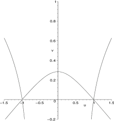
Figure 2: Plot showing the soliton $S_{12}$ disappearing from the spectrum as the $z=\mu$ vacuum crosses the curve of marginal stability in the $z$-plane. All plots have $\mu_{1}=0$ and $\mu_{2}$ is respectively $1$, $0.7$ and $0.65$. The critical value for which $\Delta=0$ if $\mu_{1}=0$ is $\mu_{2}=\pm\sqrt{2\sqrt{3}-3}\approx\pm 0.681$.

The other two soliton trajectories can be found similarly. In each case the soliton trajectory coincides with the union of the other two when $\mu_{2}\Delta=0$, although it disappears from the spectrum only on crossing the curve $\Delta=0$. It should be noted that the relevant segments of the curve $\Delta=0$ differ in all three cases. The above case, in which the 12-soliton is the one that disappears from the spectrum as we go from a ‘3-soliton’ to a ‘2-soliton’ region, corresponds to the segments with $\mu_{1}^{2}<1$, whereas the other two cases correspond to segments with $\mu_{1}^{2}>1$. We skip the details but note for future use that

$$\tan\alpha_{13}={\mu_{2}\over\mu_{1}+\Delta_{+}}\,,\qquad\tan\alpha_{23}={\mu_{2}\over\mu_{1}+\Delta_{-}}\,,$$ (16)

where

$$\Delta_{\pm}=\pm{\Delta\over 4\left[3\mu_{1}+\mu_{1}\mu_{2}^{2}-\mu_{1}^{3}\pm 2\right]}\,.$$ (17)

It follows that $\alpha_{13}=\alpha_{32}$ when $\Delta=0$, as expected.

3 The leading-order long-range force

We now plan to obtain a formula for the asymptotic force between two solitons of a (1+1)-dimensional field theory for a multi-component real scalar field $\phi(t,s)$ with Lagrangian density

$${\cal L}={1\over 2}|\dot{\phi}|^{2}-{1\over 2}|\phi^{\prime}|^{2}-V\,.$$ (18)

This of course includes (1) as a special case of a two-component real scalar field Lagrangian density. We assume that $V$ has multiple degenerate vacua at $\phi=\phi_{i}$ $(i=1,2,\dots)$, and that some vacua are connected by static soliton solutions. Let $\phi_{ij}(s)$ be a soliton connecting the $i$th vacuum to the $j$th vacuum. Near the $i$th vacuum we have

$$V\approx{1\over 2}m_{i}^{2}|\phi-\phi_{i}|^{2}\,.$$ (19)

The asymptotic form of the $ij$-soliton solution near the $j$th vacuum (as $s\rightarrow\infty$) is therefore

$$z_{ij}(s)-z_{j}\sim-m_{j}^{-1}t_{ij}e^{-m_{j}s}\,,$$ (20)

where $t_{ij}$ is tangent to the $ij$-soliton trajectory in field space as it approaches the $j$th vacuum. Similarly, the asymptotic form of the $ij$-soliton near the $i$th vacuum (as $s\rightarrow-\infty$) is

$$z_{ij}(s)-z_{i}\sim m_{i}^{-1}t_{ji}e^{m_{i}s}\,.$$ (21)

Now consider a static configuration of an $ik$-soliton at the origin, $s=0$, separated by a distance $L$ from a $kj$-soliton at $s=L$. A configuration that fits this description is

$$\phi(s)=\phi_{ik}(s)+\phi_{kj}(s-L)-\phi_{k}\,.$$ (22)

We should not expect this to be an exact solution of the field equations but it will be an approximate solution for large $L$ provided that there is a $b$ in the range $0\ll b\ll L$ such that both individual static soliton solutions $\phi_{ik}(s)$ and $\phi_{kj}(s)$ are nearly equal to their common vacuum value $\phi_{k}$ near $s=b$. We shall write (22) as

$$\phi(s)=\phi_{ik}(s)+\varphi(s)$$ (23)

where

$$\varphi(s)=\phi_{kj}(s-L)-\phi_{k}$$ (24)

and assume that $\varphi(s)$ is a small perturbation to the static solution $\phi_{ik}(s)$ in the region $s\leq b$. Since, for $s\approx b$,

$$\phi_{ik}(s)-\phi_{k}\sim-m_{k}^{-1}t_{ik}e^{-m_{k}s}\,,\qquad\varphi(s)\sim m_{k}^{-1}t_{jk}e^{m_{k}(s-L)}\,,$$ (25)

this means that we must have $2b\ll L$, so we are now assuming that

$$0\ll 2b\ll L\,.$$ (26)

The force exerted on the ik-soliton by the kj-soliton can now be found as follows [2]: the momentum of the ik-soliton is approximately given by

$$P=-\int_{-\infty}^{b}\dot{\phi}\cdot\phi^{\prime}\,ds\,.$$ (27)

The force on it is therefore

$$F\equiv\dot{P}=\left[-{1\over 2}|\dot{\phi}|^{2}-{1\over 2}|\phi^{\prime}|^{2}+V\right]_{-\infty}^{b}\,,$$ (28)

which follows on use of the field equation

$$\ddot{\phi}=\phi^{\prime\prime}-{\partial V\over\partial\phi}\,.$$ (29)

Using the ansatz (23) and properties of $\phi_{ik}$, notably

$$|\phi_{ik}^{\prime}|^{2}=2V(\phi_{ik})\,,$$ (30)

we find that

$$F=-\left[\phi_{ik}^{\prime}\cdot\varphi^{\prime}-\phi_{ik}^{\prime\prime}\cdot\varphi\,\right]_{-\infty}^{b}+{\cal O}(\varphi^{2})\,.$$ (31)

This may be evaluated using the asymptotic forms (25) of $\phi_{ik}$ and $\varphi$. The result is

$$F=-2t_{ik}\cdot t_{jk}\,e^{-m_{k}L}\,.$$ (32)

This generalizes the result of Manton to multi-component scalar field theories. For a single-component theory the tangent vectors are necessarily either parallel or antiparallel, so the force is either attractive or repulsive, never zero. For example, for a soliton-antisoliton pair we have $i=j$ and hence the attractive force [2].

$$F=-2t_{ik}^{2}e^{-m_{k}L}\,.$$ (33)

4 Application to the WZ model

The above results are applicable to the WZ model because this has degenerate vacua at critical points $z=z_{i}$ of the superpotential $W$, with

$$m_{i}^{2}=|W^{\prime}(z_{i})|^{2}\,.$$ (34)

We shall consider again the case of a quartic superpotential with critical points at $z=-1,1,\mu$ (with $\mu=\mu_{1}+i\mu_{2}$), and choose

$$\mu_{1}^{2}<1\,,$$ (35)

so that the 12-soliton is the one expected to appear as a bound state (of a 13-soliton and 32-soliton) near the curve of marginal stability. Consider a field configuration in which a 13-soliton is at $s=0$ and a 32-soliton at $s=L$, for large $L$. In the region between these solitons, and far from both, we may linearize the first-order equations (10) about the $z=\mu$ vacuum to get

$$\pmatrix{u^{\prime}\cr v^{\prime}}=\hbox{\mybb M}\pmatrix{u-\mu_{1}\cr v-\mu_{2}}$$ (36)

where the matrix 𝕄 is

$$\hbox{\mybb M}=4\pmatrix{\mu_{1}^{2}-\mu_{2}^{2}-1&2\mu_{1}\mu_{2}\cr 2\mu_{1}\mu_{2}&\mu_{1}^{2}-\mu_{2}^{2}-1}\pmatrix{\cos\alpha&\sin\alpha\cr-\sin\alpha&\cos\alpha}\,.$$ (37)

This matrix has eigenvalues $\pm m_{3}$, where

$$m_{3}=4\sqrt{1+|\mu|^{4}}\,.$$ (38)

The corresponding eigenvectors are

$$e_{\pm}(\alpha)={1\over\sqrt{2}\left[1\mp\cos(\theta+\alpha)\right]^{1\over 2}}\left(\sin(\alpha+\theta),-\cos(\alpha+\theta)\pm 1\right)$$ (39)

where

$$\tan\theta={2\mu_{1}\mu_{2}\over 1+\mu_{2}^{2}-\mu_{1}^{2}}\,.$$ (40)

These eigenvectors are tangents to the separatrix flows at $z=\mu$. Note that they are orthogonal.

The generic solution of (36) has both $e^{-m_{3}s}$ and $e^{m_{3}s}$ terms, but the asymptotic 13-soliton solution $z_{13}$ has only the $e^{-m_{3}s}$ exponential term. Thus, we should take

$$t_{13}\propto e_{-}(\alpha_{13})\,.$$ (41)

Similarly, the asymptotic 32-soliton solution, near the 3-vacuum, has only the $e^{m_{3}s}$ factor, so we should take

$$t_{23}\propto e_{+}(\alpha_{32})\,.$$ (42)

The sign of the constant of proportionality should be the same in both cases, so this yields the force

$$F\propto-\sin\left[{1\over 2}(\alpha_{13}-\alpha_{32})\right]\sin\left[{1\over 2}(\alpha_{13}+\alpha_{32})+\theta\right]+\sin^{2}\left[{1\over 2}(\alpha_{13}-\alpha_{32})\right]\,$$ (43)

for some positive constant of proportionality.

Consider first the case for which $\mu_{2}=0$, so that both soliton solutions correspond to BPS-flows along the real axis in the $z$-plane from $z=-1$ to $z=1$ (since $\mu_{1}^{2}<1$ by hypothesis). From (16) we then see that

$$\alpha_{13}=0,\pi\,.$$ (44)

Similarly for $\alpha_{32}$ but $\alpha_{32}=\alpha_{13}+\pi$. To see why, note that a BPS flow just above the real axis will approach the vacuum at $z=\mu$ anti-parallel to the real axis ($e_{-}$) and then leave it parallel to the imaginary axis ($-e_{+}$). To arrange for this flow to reach $z=1$ (or close to it) we must rotate $-e_{+}$ back to $e_{-}$. This is achieved by a shift of the angle by $\pi$ since

$$e_{\mp}(\alpha+\pi)=-e_{\pm}(\alpha)\,.$$ (45)

Thus, in this case,

$$\alpha_{32}=\alpha_{13}+\pi\,,$$ (46)

and this leads to $F\propto(1-\sin\theta)$. Since $\sin\theta=0$ for real $\mu$ we thus deduce that $F\propto 1$ with positive constant of proportionality; that is, $F>0$, so the force is repulsive, as expected.

We now turn to those cases for which $\mu$ is near the curve of marginal stability. In this case we see from (16) that

$$\left(\alpha_{13}-\alpha_{23}\right)={-\mu_{2}\Delta\over 4\mu_{1}^{2}(1-\mu_{1}^{2})^{3}}+{\cal O}\left(\Delta^{2}\right)\,.$$ (47)

It follows, after some calculation, that

$$F\propto{\mu_{2}^{2}\left(1+|\mu|^{2}\right)\left(1+\mu_{2}^{2}-\mu_{1}^{2}\right)\Delta\over(1-\mu_{1}^{2})^{3}\sqrt{\mu_{1}^{2}(1-|\mu|^{2})^{2}+\mu_{2}^{2}(1+|\mu|^{2})^{2}\left(1+\mu_{2}^{2}-\mu_{1}^{2}\right)^{2}}}+{\cal O}\left(\Delta^{2}\right)\,.$$ (48)

Since $\mu_{1}^{2}<1$, all factors other than $\Delta$ are positive. We thus have

$$F(L)\sim c^{2}\left[\Delta+{\cal O}\left(\Delta^{2}\right)\right]e^{-m_{3}L}\,,$$ (49)

for some non-zero constant $c$. The leading-order asymptotic force is therefore repulsive when $\Delta>0$, which corresponds to a point inside the ‘2-soliton’ region. It is attractive when $\Delta<0$, which corresponds to a point inside a ‘3-soliton’ region. On the curve of marginal stability the leading-order asymptotic force is zero.

5 Soliton bound states

So far, we have analysed the behaviour of solitons in the WZ model with quartic superpotential near the curve of marginal stability in the moduli space of such superpotentials. On one side of this curve there are only two types of soliton and the long-range asymptotic force between these two solitons is repulsive. We have shown, however, that this repulsive asymptotic force vanishes on the curve of marginal stability, and becomes attractive after it is crossed.

An interesting question that this result raises is whether the long-range intersoliton force vanishes on the curve of marginal stability only to leading order in an asymptotic expansion (in powers of $e^{-m_{3}L}$) or to all orders (assuming the existence of this expansion). If the force were to vanish exactly on the curve of marginal stability then we would expect to be able to find a one-parameter family of 12-soliton solutions corresponding to a 13 and 32 soliton at arbitrary separations. However, there are no such solutions because the 12-soliton trajectory necessarily coincides, on (the appropriate segment of) the curve of marginal stability, with the union of the 13 and 32-soliton trajectories. This fact suggests that it is only the leading-order asymptotic force that vanishes on the curve of marginal stability, and that the next-to-leading order term is non-zero. Given that it is non-zero it must be repulsive because an attractive force would imply a bound state ‘third soliton’ on the ‘2-soliton’ side of the curve of marginal stability. Near $\Delta=0$ we thus expect an asymptotic expansion for the intersoliton force of the form

$$F(L)\sim c^{2}\Delta e^{-m_{3}L}+\gamma^{2}e^{-2m_{3}L}+\dots$$ (50)

for some non-zero constant $\gamma$. When $\Delta<0$ this force vanishes for

$$e^{-m_{3}L}\approx\left(c^{2}/\gamma^{2}\right)|\Delta|\,.$$ (51)

Since $\Delta$ is small the neglect of the higher-order terms in (50) is justified, and there is thus a minimum of the inter-soliton potential at $L\sim(1/m_{3})\log(1/|\Delta|)$. This diverges on the curve of marginal stability, as we know must happen from the analysis of the soliton trajectories, and this explains the discontinuity of the spectrum on crossing this curve. As mentioned earlier, this result agrees qualitatively with a similar result obtained for a different scalar field model by different methods [7], as well as with results for other types of supersymmetric soliton.

Acknowledgements: We thank Jerome Gauntlett and Nick Manton for very helpful discussions. R.P. thanks Trinity College Cambridge for financial support.

References

- [1] J.P. Gauntlett, D. Tong and P.K. Townsend, Multi-domain walls in massive supersymmetric sigma models, Phys. Rev. D64 (2001) 025010.
- [2] N.S. Manton, An effective Lagrangian for solitons, Nucl. Phys. B150 (1979) 397.
- [3] P. Fendley, S.D. Mathus, C. Vafa and N.P. Warner, Integrable deformations and scattering matrices for the N=2 supersymmetric discrete series, Phys. Lett. B243 (1990) 257.
- [4] E.R.C. Abraham and P.K. Townsend, Intersecting extended objects in supersymmetric field theories, Nucl. Phys. B351 (1991) 313.
- [5] M. Cvetic, F. Quevedo and S-J. Rey, Stringy domain walls and target space modular invariance, Phys. Rev. Lett. 67. (1991) 1836.
- [6] S. Cecotti and C. Vafa, On classification of N=2 supersymmetric theories, Commun. Math. Phys. 158 (1993) 569.
- [7] A. Ritz, M. Shifman, A. Vainshtein and M. Voloshin, Marginal Stability and the metamorphosis of BPS states, Phys. Rev. D (2001) 065018.
- [8] P.C. Argyres and K. Narayan, String webs from field theory, JHEP 0103 (2001) 047.
- [9] F. Denef, B. Greene and M. Raugas, Split attractor flows and the spectrum of BPS D-branes on the quintic, JHEP 0105 (2001) 012.
- [10] A. Ritz and A. Vainshtein, Long range forces and supersymmetric bound states, Nucl. Phys. B617 (2001) 43.
- [11] N. Motoyui, S. Tominaga and M. Yamada, Hamilton-Jacobi Solution to Soliton Paths and Triangular Mass Relation in Two-dimensional Extended Supersymmetric Theory, Mod. Phys. Lett. A16 (2001) 1559.