The Principle of the
Fermionic Projector
Appendices

Preface to the Second Online Edition

In the almost twelve years since this book was completed, the fermionic projector approach evolved to what is known today as the theory of causal fermion systems. There has been progress in several directions: the mathematical setting was generalized, the mathematical methods were improved and enriched, and the physical applications have been concretized and worked out in more detail. The current status of the theory is presented in a coherent way in the recent monograph [5]. An untechnical physical introduction is given in [9].

Due to these developments, parts of the present book are superseded by the more recent research papers or the monograph [5]. However, other parts of this book have not been developed further and are still up to date. For some aspects not covered in [5], the present book is still the best reference. Furthermore, the present book is still of interest as being the first publication in which the causal action principle was presented. Indeed, comparing the presentation in the present book to the later developments should give the reader a deeper understanding of why certain constructions were modified and how they were improved. In order to facilitate such a study, we now outline the developments which led from the present book to the monograph [5]. In order not to change the original bibliography, a list of references to more recent research papers is given at the end of this preface, where numbers are used (whereas the original bibliography using letters is still at the end of the book). Similar as in the first online edition, I took the opportunity to correct a few typos. Also, I added a few footnotes beginning with “Online version:”. Apart from these changes, the online version coincides precisely with the printed book in the AMS/IP series. In particular, all equation numbers are the same.

Maybe the most important change in the mathematical setup was the move from indefinite inner product spaces to Hilbert spaces, as we now explain in detail. Clearly, the starting point of all my considerations was Dirac theory. On Dirac wave functions in Minkowski space, one can introduce the two inner products

$$(\Psi|\Phi) =\int_{\mbox{\rm\scriptsize I R}^{3}}(\overline{\Psi}\gamma^{0}\Phi)(t,\vec{x})\>d^{3}x$$ (1)

$$\mbox{$<\!\!$ \nolinebreak}\Psi|\Phi\mbox{\nolinebreak$>$} =\int_{\mbox{\rm\scriptsize I R}^{4}}\overline{\Psi(x)}\Phi(x)\>d^{4}x\>.$$ (2)

The first inner product (1) is positive definite and thus defines a scalar product. For solutions of the Dirac equation, it is time independent due to current conservation, making the solution space of the Dirac equation to a Hilbert space (more generally, the scalar product can be computed by integrating the normal component of the Dirac current over any Cauchy surface). The inner product (2), on the other hand, is indefinite. It is well-defined and covariant even on wave functions which do not satisfy the Dirac equation, giving rise to an indefinite inner product space (which can be given a Krein space structure). It should be pointed out that the time integral in (2) in general diverges for solutions of the Dirac equation, a problem which I always considered to be more of technical than of fundamental nature (this technical problem can be resolved for example by working as in (LABEL:56)–(LABEL:58) with a $\delta$-normalization in the mass parameter or by making use of the mass oscillation property as introduced in [12]).

The fermionic projector approach is based on the belief that on a microscopic scale (like the Planck scale), space-time should not be modeled by Minkowski space but should have a different, possibly discrete structure. Consequently, the Dirac equation in Minkowski space should not be considered as being fundamental, but it should be replaced by equations of different type. For such a more fundamental description, the scalar product (1) is problematic, because it is not clear how the analog of an integral over a hypersurface should be defined, and why this integral should be independent of the choice of the hypersurface. The indefinite inner product (2), however, can easily be generalized to for example a discrete space-time if one simply replaces the integral in (2) by a sum over all space-time points. Such considerations led me to regard the indefinite inner product (2) as being more fundamental than (1). This is the reason why throughout this book, we work preferably with indefinite inner product spaces. In particular, the structure of “discrete space-time” is introduced on an underlying indefinite inner product space (see §LABEL:psec13).

My views changed gradually over the past few years. The first input which triggered this process was obtained when developing the existence theory for the causal action principle. While working on this problem in the simplest setting of a finite number of space-time points [1], it became clear that in order to ensure the existence of minimizers, one needs to assume that the image of the fermionic projector $P$ is a negative definite subspace of the indefinite inner product space $(H,\mbox{$<\!\!$ \nolinebreak}.|.\mbox{\nolinebreak$>$})$. The fact that $P$ has a definite image makes it possible to introduce a Hilbert space $(\mathscr{H},\langle.|.\rangle_{\mathscr{H}})$ by setting $\langle.|.\rangle_{\mathscr{H}}=-\mbox{$<\!\!$ \nolinebreak}.|P\,.\mbox{\nolinebreak$>$}$ and dividing out the null space. This construction, which was first given in [7, Section 1.2.2], gave an underlying Hilbert space structure. However, at this time, the connection of the corresponding scalar product to integrals over hypersurfaces as in (1) remained obscure.

From the mathematical point of view, having an underlying Hilbert space structure has the major benefit that functional analytic methods in Hilbert spaces become applicable. When thinking about how to apply these methods, it became clear that also measure-theoretic methods are useful. This led me to generalize the mathematical setting such as to allow for the description of not only discrete, but also continuous space-times. This setting was first introduced in [3] when working out the existence theory. This analysis also clarified which constraints one must impose in order to obtain a mathematically well-posed variational problem.

The constructions in [3] also inspired the notion of the universal measure, as we now outline. When working out the existence theory, it became clear that instead of using the kernel of the fermionic projector, the causal action principle can be formulated equivalently in terms of the local correlation operators $F(x)$ which relate the Hilbert space scalar product to the spin scalar product by

$$\langle\psi|F(x)\phi\rangle_{\mathscr{H}}=-\mbox{$\prec\!\!$ \nolinebreak}\psi(x)|\phi(x)\mbox{\nolinebreak$\succ$}_{x}\>.$$

In this formulation, the only a-priori structure of space-time is that of being a measure space $(M,\mu)$. The local correlation operators give rise to a mapping

$$F\>:\>M\rightarrow{\mathscr{F}}\>,\quad x\mapsto F(x)\>,$$

where ${\mathscr{F}}$ is the subset of finite rank operators on $\mathscr{H}$ which are symmetric and (counting multiplicities) have at most $2N$ positive and at most $2N$ negative eigenvalues (where $N$ denotes the number of sectors). Then, instead of working with the measure $\mu$, the causal action can be expressed in terms of the push-forward measure $\rho=F_{*}\mu$, being a measure on ${\mathscr{F}}$ (defined by $\rho(\Omega)=\mu(F^{-1}(\Omega))$). As a consequence, it seems natural to leave out the measure space $(M,\mu)$ and to work instead directly with the measure $\rho$ on ${\mathscr{F}}$, referred to as the universal measure. We remark that working with $(M,\mu)$ has the potential benefit that it is possible to prescribe properties of the measure $\rho$. In particular, if $\mu$ is a discrete measure, then so is $\rho$ (for details see [3, Section 1.2]). However, the analysis of the causal action principle in [13] suggests that minimizing measures are always discrete, even if one varies over all regular Borel measures (which may have discrete and continuous components). With this in mind, it seems unnecessary to arrange the discreteness of the measure $\rho$ by starting with a discrete measure space $(M,\mu)$. Then the measure space $(M,\mu)$ becomes obsolete. These considerations led me to the conviction that one should work with the universal measure $\rho$, which should be varied within the class of all regular Borel measures. Working with general regular Borel measures also has the advantage that it becomes possible to take convex combinations of universal measures, which seems essential for getting the connection to second-quantized bosonic fields (see the notions of decoherent replicas of space-time and of microscopic mixing of wave functions in [4] and [15]).

Combining all the above results led to the framework of causal fermion systems, where a physical system is described by a Hilbert space $(\mathscr{H},\langle.|.\rangle_{\mathscr{H}})$ and the universal measure $\rho$ on ${\mathscr{F}}$. This framework was first introduced in [7]. Subsequently, the analytic, geometric and topological structures encoded in a causal fermion system were worked out systematically; for an overview see [5, Chapter 1].

From the conceptual point of view, the setting of causal fermion systems and the notion of the universal measure considerably changed both the role of the causal action principle and the concept of what space-time is. Namely, in the causal action principle in this book, one varies the fermionic projector $P$ in a given discrete space-time. In the setting of causal fermion systems, however, one varies instead the universal measure $\rho$, being a measure on linear operators on an abstract Hilbert space. In the latter formulation, there is no space-time to begin with. On the contrary, space-time is introduced later as the support of the universal measure. In this way, the causal action principle evolved from a variational principle for wave functions in space-time to a variational principle for space-time itself as well as for all structures therein.

In order to complete the summary of the conceptual modifications, we remark that the connection between the scalar product $\langle.|.\rangle_{\mathscr{H}}$ and surface integrals as in (1), which had been obscure for quite a while, was finally clarified when working out Noether-like theorems for causal variational principles [10]. Namely, surface integrals now have a proper generalization to causal fermion systems in terms of so-called surface layer integrals. It was shown that the symmetry of the causal action under unitary transformations acting on $\mathscr{F}$ gives rise to conserved charges which can be expressed by surface layer integrals. For Dirac sea configurations, these conserved charges coincide with the surface integrals (1).

Another major development concerns the description of neutrinos. In order to explain how these developments came about, we first note that in this book, neutrinos are modelled as left-handed massless Dirac particles (see §LABEL:esec1). This has the benefit that the neutrinos drop out of the closed chain due to chiral cancellations (see §LABEL:esec21 and §LABEL:esec22). When writing this book, I liked chiral cancellations, and I even regarded them as a possible explanation for the fact that neutrinos appear only with one chirality. As a side remark, I would like to mention that I was never concerned about experimental observations which indicate that neutrinos do have a rest mass, because I felt that these experiments are too indirect for making a clear case. Namely, measurements only tell us that there are fewer neutrinos on earth than expected from the number of neutrinos generated in fusion processes in the sun. The conventional explanation for this seeming disappearance of solar neutrinos is via neutrino oscillations, making it necessary to consider massive neutrinos. However, it always seemed to me that there could be other explanations for the lack of neutrinos on earth (for example, a modification of the weak interaction or other, yet unknown fundamental forces), in which case the neutrinos could well be massless.

My motivation for departing from massless neutrinos was not related to experimental evidence, but had to do with problems of mathematical consistency. Namely, I noticed that left-handed neutrinos do not give rise to stable minimizers of the causal action (see [5, Section 4.2]). This general result led me to incorporate right-handed neutrino components, and to explain the fact that only the left-handed component is observed by the postulate that the regularization breaks the chiral symmetry. This procedure cured the mathematical consistency problems and had the desired side effect that neutrinos could have a rest mass, in agreement with neutrino oscillations.

We now comment on other developments which are of more technical nature. These developments were mainly triggered by minor errors or shortcomings in the present book. First, Andreas Grotz noticed when working on his master thesis in 2007 that the normalization conditions for the fermionic projector as given in (LABEL:eq:2a1) and (LABEL:eq:2a2) are in general violated to higher order in perturbation theory. This error was corrected in [6] by a rescaling procedure. This construction showed that there are two different perturbation expansions: with and without rescaling. The deeper meaning of these two expansions became clearer later when working out different normalizations of the fermionic projector. This study was initiated by the quest for a non-perturbative construction of the fermionic projector, as was carried out in globally hyperbolic space-times in [11, 12]. It turned out that in space-times of finite lifetime, one cannot work with the $\delta$-normalization in the mass parameter as used in (LABEL:56)–(LABEL:58) (the “mass normalization”). Instead, a proper normalization is obtained by using a scalar product $(.|.)$ which is represented similar to (1) by an integral over a spacelike hypersurface (the “spatial normalization”). As worked out in detail in [14] with a convenient contour integral method, the causal perturbation expansion without rescaling realizes the spatial normalization condition, whereas the rescaling procedure in [6] gives rise to the mass normalization. The constructions in curved space-time in [11, 12] as well as the general connection between the scalar product $(.|.)$ and the surface layer integrals in [10] showed that the physically correct and mathematically consistent normalization condition is the spatial normalization condition. With this in mind, the combinatorics of the causal perturbation expansion in this book is indeed correct, but the resulting fermionic projector does not satisfy the mass but the spatial normalization condition.

Clearly, the analysis of the continuum limit in Chapters LABEL:esec3–LABEL:esec5 is superseded by the much more detailed analysis in [5, Chapters 3-5]. A major change concerns the treatment of the logarithmic singularities on the light cone, as we now point out. In the present book, some of the contributions involving logarithms are arranged to vanish by imposing that the regularization should satisfy the relation (LABEL:e:3C). I tried for quite a while to construct an example of a regularization which realizes this relation, until I finally realized that there is no such regularization, for the following reason:

Lemma I. There is no regularization which satisfies the condition (LABEL:e:3C).

Proof. The linear combination of monomials $M$ in (LABEL:e:3B) involves a factor $T^{(1)}_{[2]}$, which has a logarithmic pole on the light cone (see (LABEL:Tldef), (LABEL:Tadef) and (LABEL:l:3.1)). Restricting attention to the corresponding contribution $\sim\log|\vec{\xi}|$, we have

$$M\asymp-\frac{1}{16\pi^{3}}\>T^{(-1)}_{[0]}\>\overline{T^{(-1)}_{[0]}\>T^{(0)}_{[0]}}\>\log|\vec{\xi}|\>.$$

As a consequence,

$$(M -\overline{M})\>\overline{T^{(0)}_{[0]}}^{-1}=-\frac{\log|\vec{\xi}|}{16\pi^{3}}\>\frac{\big{|}T^{(-1)}_{[0]}\big{|}^{2}}{\overline{T^{(0)}_{[0]}}}\big{(}\overline{T^{(0)}_{[0]}}-T^{(0)}_{[0]}\big{)}$$

$$=-\frac{\log|\vec{\xi}|}{16\pi^{3}}\>\bigg{|}\frac{T^{(-1)}_{[0]}}{T^{(0)}_{[0]}}\bigg{|}^{2}\Big{(}\big{|}T^{(0)}_{[0]}\big{|}^{2}-\big{(}T^{(0)}_{[0]}\big{)}^{2}\Big{)}=-\frac{\log|\vec{\xi}|}{8\pi^{3}}\>\bigg{|}\frac{T^{(-1)}_{[0]}}{T^{(0)}_{[0]}}\bigg{|}^{2}\,\Big{(}\text{Im}\,T^{(0)}_{[0]}\Big{)}^{2}\leq 0\>.$$

Since this expression has a fixed sign, it vanishes in a weak evaluation on the light cone only if it vanishes identically to the required degree. According to (LABEL:l:3.1), the function $\text{Im}\,T^{(0)}_{[0]}$ is a regularization of the distribution $-i\pi\delta(\xi^{2})\>\varepsilon(\xi^{0})/(8\pi^{3})$ on the scale $\varepsilon$. Hence on the light cone it is of the order $\varepsilon^{-1}$. This gives the claim.    
This no-go result led me to reconsider the whole procedure of the continuum limit. At the same time, I tried to avoid imposing relations between the regularization parameters, which I never felt comfortable with because I wanted the continuum limit to work for at least a generic class of regularizations. Resolving this important issue took me a lot of time and effort. My considerations eventually led to the method of compensating the logarithmic poles by a microlocal chiral transformation. These construction as well as many preliminary considerations are given in [5, Section 3.7].

Finally, I would like to make a few comments on each chapter of the book. Chapters LABEL:secintro–LABEL:secpfp are still up to date, except for the generalizations and modifications mentioned above. Compared to the presentation in [5], I see the benefit that these chapters might be easier to read and might convey a more intuitive picture of the underlying physical ideas. Chapter LABEL:psec2 is still the best reference for the general derivation of the formalism of the continuum limit. In [5, Chapter 2] I merely explained the regularization effects in examples and gave an overview of the methods and results in Chapter LABEL:psec2, but without repeating the detailed constructions. Chapter LABEL:esec2 is still the only reference where the form of the causal action is motivated and derived step by step. Also, the notion of state stability is introduced in detail, thus providing the basis for the later analysis in [2, 8]. As already mentioned above, the analysis in Chapters LABEL:esec3–LABEL:secegg is outdated. I recommend the reader to study instead [5, Chapters 3–5]. The Appendices are still valuable. I added a few footnotes which point to later improvements and further developments.
          Felix Finster, Regensburg, August 2016

References

Appendix A Connection to the Fock Space Formalism

In this appendix it is shown that for an observer who is making measurements only in a subsystem of the whole physical system, the description of a many-fermion system with the fermionic projector is equivalent to the fermionic Fock space formalism, provided that the number of fermions of the whole system (including the particles of the sea) is infinite. The following consideration applies in the same way to either a space-time continuum or to discrete space-time. Before beginning we point out that the action principle, from which the fundamental physical equations can be deduced, involves the fermions only via the Dirac action $\mbox{$<\!\!$ \nolinebreak}\Psi,(i\mbox{$\partial$ $/$}+{\mathcal{B}}-m)\Psi\mbox{\nolinebreak$>$}$. For the formulation of the Dirac action one only needs on the fermionic Fock space the time/position operators and the operator $\partial$ $/$, which are all one-particle operators. Therefore, we can say that many-particle operators (like for example in the four-fermion coupling of the Fermi model) are not essential for the formulation of the quantum field theory of the standard model. Having this in mind, we may here restrict attention to one-particle operators.

Let $P$ be a fermionic projector acting on the vector space $H$. The one-particle observables correspond to operators ${\mathcal{O}}$ on $H$. Our subsystem is described by a non-degenerate subspace $K\subset H$; we decompose $H$ as a direct sum $H=K\oplus L$ with $L=K^{\perp}$. We assume that the observables are localized in $N$; i.e. they are trivial on $L$,

$${\mathcal{O}}_{|L}\;=\;0_{|L}\>.$$ (A.1)

We choose a (properly normalized) basis $\Psi_{1},\ldots,\Psi_{n}$ of the subspace $P(H)\subset H$, and decompose the states $\Psi_{j}$ in the form

$$\Psi_{j}\;=\;\Psi_{j}^{K}+\Psi_{j}^{L}\;\;\;\;\;\;\;\;\;\;{\mbox{with $\Psi_{j}^{K}\in K,\Psi_{j}^{L}\in L$}}.$$

Substituting into (LABEL:p:1_16), we obtain for the many-particle wave function the expression

$$\Psi\;=\;\sum_{\pi\in{\mathcal{P}}(n)}(-1)^{|\pi|}\left(\bigwedge_{j\in\pi}\Psi_{j}^{K}\right)\land\left(\bigwedge_{j\not\in\pi}\Psi_{j}^{L}\right),$$ (A.2)

where ${\mathcal{P}}(n)$ denotes the set of all subsets of $\{1,\ldots,n\}$. For measurements in our subsystem, we must calculate the expectation value $\mbox{$<\!\!$ \nolinebreak}\Psi|{\mathcal{O}}|\Psi\mbox{\nolinebreak$>$}_{F}$, where the operators ${\mathcal{O}}$ act on the Fock space according to

$${\mathcal{O}}(\Psi_{1}\land\cdots\land\Psi_{n})\;=\;({\mathcal{O}}\Psi_{1})\land\cdots\land\Psi_{n}\>+\>\Psi_{1}\land({\mathcal{O}}\Psi_{2})\cdots\land\Psi_{n}\>+\cdots+\>\Psi_{1}\land\cdots\land({\mathcal{O}}\Psi_{n})\>,$$

and where $\mbox{$<\!\!$ \nolinebreak}.|.\mbox{\nolinebreak$>$}_{F}$ is the scalar product on the Fock space, induced by the scalar product $\mbox{$<\!\!$ \nolinebreak}.|.\mbox{\nolinebreak$>$}$ on $H$. It is useful to rewrite the expectation value with the statistical operator $S$, i.e.

$$\mbox{$<\!\!$ \nolinebreak}\Psi|{\mathcal{O}}|\Psi\mbox{\nolinebreak$>$}_{F}\;=\;\mbox{tr\/}_{F}(S\>{\mathcal{O}})\quad{\mbox{with}}\quad S\;=\;|\Psi\mbox{\nolinebreak$>$}\mbox{$<\!\!$ \nolinebreak}\Psi|_{F}\>,$$

where $\mbox{tr\/}_{F}$ denotes the trace in the Fock space. Using (A.1), we can take the partial trace over $L$ and obtain, applying (A.2),

$$\mbox{$<\!\!$ \nolinebreak}\Psi|{\mathcal{O}}|\Psi\mbox{\nolinebreak$>$}_{F} = \mbox{tr\/}_{F_{K}}(S^{K}\>{\mathcal{O}})\;\;\;\;\;\;\;\;\;\;{\mbox{with}}$$ (A.3)

$$S^{K} = \sum_{k=0}^{n}\sum_{\scriptsize\begin{array}[]{cc}\scriptsize\pi,\pi^{\prime}\in{\mathcal{P}}(n),\\ \#\pi=\#\pi^{\prime}=k\end{array}}c_{\pi,\pi^{\prime}}\;|\land_{i\in\pi}\Psi_{i}^{K}\mbox{\nolinebreak$>$}\mbox{$<\!\!$ \nolinebreak}\land_{j\in\pi^{\prime}}\Psi_{j}^{K}|_{F_{K}}$$ (A.6)

$$c_{\pi,\pi^{\prime}} = (-1)^{|\pi|+|\pi^{\prime}|}\;\mbox{$<\!\!$ \nolinebreak}\land_{i\not\in\pi}\Psi_{i}^{L}|\land_{j\not\in\pi^{\prime}}\Psi_{j}^{L}\mbox{\nolinebreak$>$}_{F}\>,$$

where $\mbox{tr\/}_{F_{K}}$ is the trace in the Fock space $F_{K}=\oplus_{k=0}^{\infty}\land^{k}K$ generated by $K$. Thus our subsystem is described by a statistical operator $S^{K}$ on $F_{K}$, which is composed of mixed states consisting of different numbers of particles. Since the constants $c_{\pi,\pi^{\prime}}$ depend on the wave functions $\Psi^{L}$ outside our subsystem, we can consider them as arbitrary numbers.

In the limit when the number $n$ of particles of the whole system tends to infinity, (A.6) goes over to a statistical operator of the form

$$S^{K}\;=\;\sum_{k=0}^{\infty}\;\sum_{\alpha,\beta=0}^{\infty}c^{(k)}_{\alpha\beta}\;|\Psi^{(k)}_{\alpha}\mbox{\nolinebreak$>$}\mbox{$<\!\!$ \nolinebreak}\Psi^{(k)}_{\beta}|_{F_{K}}$$ (A.7)

with arbitrary complex coefficients $c^{(k)}_{\alpha\beta}$ and $k$-particle states $\Psi^{(k)}_{\alpha}\in F^{k}_{K}$. This statistical operator differs from a general statistical operator $S^{K}_{\mbox{\scriptsize{gen}}}$ in that it is diagonal on the $k$-particle subspaces (i.e. that the wave functions in the “bra” and in the “ket” of (A.7) are both $k$-particle states); more precisely, $S^{K}_{\mbox{\scriptsize{gen}}}$ has, compared to (A.7), the more general form

$$S^{K}_{\mbox{\scriptsize{gen}}}\;=\;\sum_{k,l=0}^{\infty}\;\sum_{\alpha,\beta=0}^{\infty}c^{(k,l)}_{\alpha\beta}\;|\Psi^{(k)}_{\alpha}\mbox{\nolinebreak$>$}\mbox{$<\!\!$ \nolinebreak}\Psi^{(l)}_{\beta}|_{F_{K}}\>.$$ (A.8)

We remark for clarity that a pure state of the Fock space $\Psi\in F_{K}$ has a decomposition $\Psi=\sum_{k=0}^{\infty}\lambda_{k}\Psi^{(k)}$, and thus the corresponding statistical operator is

$$S\;=\;|\Psi\mbox{\nolinebreak$>$}\mbox{$<\!\!$ \nolinebreak}\Psi|_{F_{K}}\;=\;\sum_{k,l=0}^{\infty}\lambda_{k}\>\overline{\lambda_{l}}\;|\Psi^{(k)}\mbox{\nolinebreak$>$}\mbox{$<\!\!$ \nolinebreak}\Psi^{(l)}|_{F_{K}}\>.$$

This statistical operator is a special case of (A.8), but it is not of the form (A.7).

The difference between (A.7) and (A.8) becomes irrelevant if we keep in mind that all physically relevant observables commute with the particle number operator. Namely in this case, every expectation value reduces to the sum of the expectation values in the $k$-particle Fock spaces,

$$\mbox{tr\/}_{F_{K}}(S^{K}_{\mbox{\scriptsize{gen}}}\>{\mathcal{O}}) = \sum_{k,l=0}^{\infty}\;\sum_{\alpha,\beta=0}^{\infty}c^{(k,l)}_{\alpha\beta}\;\mbox{$<\!\!$ \nolinebreak}\Psi^{(l)}_{\beta}\>|\>{\mathcal{O}}\>|\>\Psi^{(k)}_{\alpha}\mbox{\nolinebreak$>$}_{F_{K}}$$

$$= \sum_{k=0}^{\infty}\;\sum_{\alpha,\beta=0}^{\infty}c^{(k,k)}_{\alpha\beta}\;\mbox{$<\!\!$ \nolinebreak}\Psi^{(k)}_{\beta}\>|\>{\mathcal{O}}\>|\>\Psi^{(k)}_{\alpha}\mbox{\nolinebreak$>$}_{F_{K}}\>.$$

If we choose the coefficients $c^{(k)}_{\alpha\beta}$ in (A.7) to be $c^{(k)}_{\alpha\beta}=c^{(k,k)}_{\alpha\beta}$, these expectation values are also obtained from the statistical operator $S^{K}$,

$$\mbox{tr\/}_{F_{K}}(S^{K}_{\mbox{\scriptsize{gen}}}\>{\mathcal{O}})\;=\;\mbox{tr\/}_{F_{K}}(S^{K}\>{\mathcal{O}})\>.$$

We conclude that it is no loss of generality to describe the subsystem by the statistical operator $S^{K}$.

Appendix B Some Formulas of the Light-Cone Expansion

This appendix is a compilation of some formulas of the light-cone expansion. More precisely, we list the phase-free contribution to the light-cone expansion of the Green’s functions (cf. Def. LABEL:l:def_pf). According to Def. LABEL:l:def_pf and Theorem LABEL:l:thm3, the light-cone expansion of the Green’s functions is immediately obtained by inserting ordered exponentials into the line integrals. Furthermore, as explained after (LABEL:fprep), the formulas can be applied directly to the fermionic projector; they then describe the singularities of $\tilde{P}(x,y)$ on the light cone. Without loss of generality, we restrict attention to the left handed component of the Green’s functions. We compute precisely those contributions which will be of relevance in Appendix G and in Chapters LABEL:esec3–LABEL:esec5. The following formulas were all generated by a computer program, see [F6] for details.

We begin with the perturbation by a chiral perturbation to first order. The phase-free contribution (denoted by a corresponding superscript on the equal sign) is

$$\chi_{L}\>(-s\>(\chi_{L}\mbox{ $\!\!A$ $/$}_{R}+\chi_{R}\mbox{ $\!\!A$ $/$}_{L})\>s)(x,y)\;\stackrel{{\scriptstyle\mbox{\footnotesize{phase-free}}}}{{=}}\;\xi\mbox{ $/$}\>{\mathcal{O}}((y-x)^{0})+{\mathcal{O}}((y-x)^{2})$$ (B.9)

$$+\chi_{L}\>S^{(0)}(x,y)\>\xi^{i}\int_{x}^{y}dz\>[0,1\>|\>0]\>(\mbox{$\partial$ $/$}A_{Li})$$

$$-\chi_{L}\>S^{(0)}(x,y)\>\int_{x}^{y}dz\>[0,0\>|\>0]\>\mbox{ $\!\!A$ $/$}_{L}$$

$$+\chi_{L}\>S^{(0)}(x,y)\>\mbox{ $\!\!A$ $/$}_{L}(x)$$

$$+\frac{1}{2}\>\chi_{L}\>S^{(0)}(x,y)\>\xi\mbox{ $/$}\int_{x}^{y}dz\>[0,0\>|\>0]\>(\mbox{$\partial$ $/$}\mbox{ $\!\!A$ $/$}_{L})$$

$$-\chi_{L}\>S^{(0)}(x,y)\>\xi\mbox{ $/$}\>\int_{x}^{y}dz\>[1,0\>|\>0]\>(\partial^{i}A_{Li})$$

$$+\frac{1}{2}\chi_{L}\>S^{(0)}(x,y)\>\xi\mbox{ $/$}\>\xi^{i}\>\int_{x}^{y}dz\>[0,0\>|\>1]\>(\raisebox{2.58334pt}{\framebox{}}\,A_{Li})$$

$$+\chi_{L}\>S^{(1)}(x,y)\>\xi^{i}\>\int_{x}^{y}dz\>[0,1\>|\>1]\>(\mbox{$\partial$ $/$}\raisebox{2.58334pt}{\framebox{}}\,A_{Li})$$

$$+\chi_{L}\>S^{(1)}(x,y)\>\int_{x}^{y}dz\>[0,2\>|\>0]\>(\raisebox{2.58334pt}{\framebox{}}\,\mbox{ $\!\!A$ $/$}_{L})$$

$$-2\chi_{L}\>S^{(1)}(x,y)\>\int_{x}^{y}dz\>[0,0\>|\>1]\>(\mbox{$\partial$ $/$}\partial^{i}A_{Li})\>,\;\;\;\;\;\;\;\;\;\;\;\;\;\;\;\;\;\;\;\;\;\;\;\;\;\;\;\;\;\;\quad$$

where again $\xi\equiv(y-x)$. The notation $\xi\mbox{ $/$}\>{\mathcal{O}}((y-x)^{2})$ means that we leave out all contributions which are of the order ${\mathcal{O}}((y-x)^{0})$ and have a leading factor $\xi\mbox{ $/$}$. This formula has the disadvantage that it contains partial derivatives of the chiral potential; it would be better for physical applications to work instead with the Yang-Mills field tensor and the Yang-Mills current. Therefore, we introduce left and right handed gauge-covariant derivatives $D^{L\!/\!R}$,

$$D^{L}_{j}\;=\;\frac{\partial}{\partial x^{j}}\>-\>iA_{Lj}\>,\;\;\;\;\;\;\;\;\;\;D^{R}_{j}\;=\;\frac{\partial}{\partial x^{j}}\>-\>iA_{Rj}\>,$$

and define the corresponding field tensor and current as usual by the commutators

$$F^{c}_{jk}\;=\;i\left[D^{c}_{j},\>D^{c}_{k}\right]\>,\;\;\;\;\;\;\;\;\;\;j^{c}_{l}\;=\;\left[D^{c\>k},\>F^{c}_{lk}\right]\;\;\;\;\;\;\;\;\;\;{\mbox{($c=L$ or $R$)}}.$$ (B.10)

In the case of an Abelian gauge field, this formula reduces to the familiar formulas for the electromagnetic field tensor and current,

$$F^{c}_{jk}\;=\;\partial_{j}A_{c\>k}-\partial_{k}A_{c\>j}\>,\;\;\;\;\;\;\;\;\;\;j^{c}_{l}\;=\;\partial_{lk}A^{k}_{c}-\raisebox{2.58334pt}{\framebox{}}\,A_{c\>l}\>.$$

Notice, however, that in the general case of a system of Dirac seas, (B.10) involves quadratic and cubic terms in the potential.

By substituting (B.10) into (B.9–B.9) and manipulating the line integrals with integrations by parts, one can rewrite the phase-free contribution in a way where the linear terms in the potential are gauge invariant. For example, we can combine (B.9–B.9) by transforming the line integrals as

$$\xi^{k}\int_{x}^{y}dz\>[0,1\>|\>0]\>(\mbox{$\partial$ $/$}A_{Lk})\;=\;\xi^{k}\int_{x}^{y}dz\>[0,1\>|\>0]\>(\gamma^{j}F^{L}_{jk}\>+\>\partial_{k}\mbox{ $\!\!A$ $/$}_{L})\>+\>{\mathcal{O}}(A_{L}^{2})$$ (B.11)

$$= \xi^{k}\int_{x}^{y}dz\>[0,1\>|\>0]\>\gamma^{j}F^{L}_{jk}\>-\>\mbox{ $\!\!A$ $/$}_{L}(x)\>+\>\int_{x}^{y}dz\>[0,0\>|\>0]\>\mbox{ $\!\!A$ $/$}_{L}\>+\>{\mathcal{O}}(A_{L}^{2})\>.\;\;\;\;\;\;\;\;\;\;$$

This procedure yields (in the non-Abelian case) quadratic and cubic terms in the potential which are not gauge invariant. Fortunately, these gauge-dependent terms are all compensated by corresponding contributions to the higher order Feynman diagrams. We thus obtain

$$\chi_{L}\sum_{k=0}^{\infty}((-s\>(\chi_{L}\mbox{ $\!\!A$ $/$}_{R}+\chi_{R}\mbox{ $\!\!A$ $/$}_{L}))^{k}\>s)(x,y)\;\stackrel{{\scriptstyle\mbox{\footnotesize{phase-free}}}}{{=}}\;\xi\mbox{ $/$}\>{\mathcal{O}}((y-x)^{0})+{\mathcal{O}}((y-x)^{2})$$

$$+\chi_{L}\>S^{(0)}(x,y)\>\xi^{i}\int_{x}^{y}dz\>[0,1\>|\>0]\>\gamma^{l}F^{L}_{li}$$

$$+\frac{1}{4}\>\chi_{L}\>S^{(0)}(x,y)\>\xi\mbox{ $/$}\>\int_{x}^{y}dz\>[0,0\>|\>0]\>\gamma^{j}\gamma^{k}\>F^{L}_{jk}$$

$$-\frac{1}{2}\>\chi_{L}\>S^{(0)}(x,y)\>\xi\mbox{ $/$}\>\xi^{i}\int_{x}^{y}dz\>[0,0\>|\>1]\>j^{L}_{i}$$

$$-i\chi_{L}\>S^{(0)}(x,y)\>\xi\mbox{ $/$}\>\xi_{i}\xi^{j}\int_{x}^{y}dz_{1}\>[0,1\>|\>1]\>F^{L}_{kj}\int_{z_{1}}^{y}dz_{2}\>[0,1\>|\>0]\>F_{L}^{ki}$$

$$+\chi_{L}\>S^{(1)}(x,y)\>\xi^{i}\int_{x}^{y}dz\>[0,1\>|\>1]\>(\mbox{$\partial$ $/$}j^{L}_{i})$$

$$+\chi_{L}\>S^{(1)}(x,y)\>\int_{x}^{y}dz\>[0,2\>|\>0]\>j^{L}_{k}\>\gamma^{k}$$

$$-i\chi_{L}\>S^{(0)}(x,y)\>\xi\mbox{ $/$}\>\xi_{i}\xi^{j}\int_{x}^{y}dz_{1}\>[0,1\>|\>1]\>F^{L}_{kj}\int_{z_{1}}^{y}dz_{2}\>[0,1\>|\>0]\>F_{L}^{ki}$$

$$+i\chi_{L}\>S^{(1)}(x,y)\>\xi^{i}\xi^{j}\int_{x}^{y}dz_{1}\>[0,3\>|\>0]\>\gamma^{k}\>F^{L}_{kj}\int_{z_{1}}^{y}dz_{2}\>[0,0\>|\>1]\>j^{L}_{i}$$

$$+i\chi_{L}\>S^{(1)}(x,y)\>\xi^{i}\xi^{j}\int_{x}^{y}dz_{1}\>[0,2\>|\>1]\>j^{L}_{j}\int_{z_{1}}^{y}dz_{2}\>[0,1\>|\>0]\>\gamma^{l}\>F^{L}_{li}$$

$$-2i\chi_{L}\>S^{(1)}(x,y)\>\xi_{i}\xi^{j}\int_{x}^{y}dz_{1}\>[0,2\>|\>1]\>F^{L}_{mj}\int_{z_{1}}^{y}dz_{2}\>[0,2\>|\>0]\>(\mbox{$\partial$ $/$}F_{L}^{mi})$$

$$-2i\chi_{L}\>S^{(1)}(x,y)\>\xi_{i}\xi^{j}\int_{x}^{y}dz_{1}\>[0,2\>|\>1]\>(\mbox{$\partial$ $/$}F^{L}_{kj})\int_{z_{1}}^{y}dz_{2}\>[0,1\>|\>0]\>F_{L}^{ki}$$

$$+i\chi_{L}\>S^{(1)}(x,y)\>\xi^{i}\xi^{j}\int_{x}^{y}dz_{1}\>[0,2\>|\>1]\>\gamma^{k}F^{L}_{kj}\int_{z_{1}}^{y}dz_{2}\>[0,2\>|\>0]\>j^{L}_{i}$$

$$-\frac{i}{2}\>\chi_{L}\>S^{(1)}(x,y)\>\xi^{i}\int_{x}^{y}dz_{1}\>[0,2\>|\>0]\>\gamma^{j}F^{L}_{ji}\int_{z_{1}}^{y}dz_{2}\>[0,0\>|\>0]\>\gamma^{k}\gamma^{l}F^{L}_{kl}$$

$$-\frac{i}{2}\>\chi_{L}\>S^{(1)}(x,y)\>\xi^{i}\int_{x}^{y}dz_{1}\>[0,2\>|\>0]\>\gamma^{j}\gamma^{k}F^{L}_{jk}\int_{z_{1}}^{y}dz_{2}\>[0,1\>|\>0]\>\gamma^{l}F^{L}_{li}$$

$$+2i\chi_{L}\>S^{(1)}(x,y)\>\xi_{i}\int_{x}^{y}dz_{1}\>[0,3\>|\>0]\>\gamma^{j}F^{L}_{jk}\int_{z_{1}}^{y}dz_{2}\>[0,1\>|\>0]\>F_{L}^{ki}$$

$$-2i\chi_{L}\>S^{(1)}(x,y)\>\xi^{j}\int_{x}^{y}dz_{1}\>[0,1\>|\>1]\>F^{L}_{ij}\int_{z_{1}}^{y}dz_{2}\>[0,1\>|\>0]\>\gamma_{k}F_{L}^{ki}$$

$$-2\chi_{L}\>S^{(1)}(x,y)\>\xi_{i}\xi^{j}\xi^{k}$$

$$\quad\times\int_{x}^{y}dz_{1}\>[0,4\>|\>0]\>\gamma^{l}F^{L}_{lk}\int_{z_{1}}^{y}dz_{2}\>[0,1\>|\>1]\>F^{L}_{mj}\int_{z_{2}}^{y}dz_{3}\>[0,1\>|\>0]\>F_{L}^{mi}$$

$$-2\chi_{L}\>S^{(1)}(x,y)\>\xi_{i}\xi^{j}\xi^{k}$$

$$\quad\times\int_{x}^{y}dz_{1}\>[0,3\>|\>1]\>\gamma^{l}F^{L}_{lk}\int_{z_{1}}^{y}dz_{2}\>[0,3\>|\>0]\>F^{L}_{mj}\int_{z_{2}}^{y}dz_{3}\>[0,1\>|\>0]\>F_{L}^{mi}$$

$$-2\chi_{L}\>S^{(1)}(x,y)\>\xi_{i}\xi^{j}\xi^{k}$$

$$\quad\times\int_{x}^{y}dz_{1}\>[0,3\>|\>1]\>F^{L}_{mk}\int_{z_{1}}^{y}dz_{2}\>[0,3\>|\>0]\>\gamma^{l}F^{L}_{lj}\int_{z_{2}}^{y}dz_{3}\>[0,1\>|\>0]\>F_{L}^{mi}$$

$$-2\chi_{L}\>S^{(1)}(x,y)\>\xi^{i}\xi_{j}\xi^{k}$$

$$\quad\times\int_{x}^{y}dz_{1}\>[0,3\>|\>1]\>F^{L}_{mk}\int_{z_{1}}^{y}dz_{2}\>[0,3\>|\>0]\>F_{L}^{mj}\int_{z_{2}}^{y}dz_{3}\>[0,1\>|\>0]\>\gamma^{l}F^{L}_{li}\>.\;\;\;\;\;\;\;\;\;\;$$

We call this formulation of the phase-free contributions purely in terms of the Yang-Mills field tensor and the Yang-Mills current the gauge invariant form of the light-cone expansion.

It remains to consider the scalar/pseudoscalar perturbation; i.e. we must study how the dynamic mass matrices $Y_{L\!/\!R}(x)$ show up in the light-cone expansion. We begin with the case of a single mass matrix. To first order in the external potential, the corresponding Feynman diagram has the light-cone expansion

$$\chi_{L}\>m\>(-s\>(-\chi_{L}Y_{R}-\chi_{R}Y_{L})\>s)(x,y)$$ (B.12)

$$\stackrel{{\scriptstyle\mbox{\footnotesize{phase-free}}}}{{=}} \frac{1}{2}\>\chi_{L}\>m\>S^{(0)}(x,y)\>\xi\mbox{ $/$}\>\int_{x}^{y}dz\>[0,0\>|\>0]\>(\mbox{$\partial$ $/$}Y_{L})$$

$$+\chi_{L}\>m\>S^{(0)}(x,y)\>Y_{L}(x)\>+\>{\mathcal{O}}((y-x)^{0})\>.$$

The higher orders in the chiral potentials yield no phase-free contributions. The next orders in the mass parameter are treated similarly. The contributions quadratic in $m$ are

$$\chi_{L}\>m^{2}\>\sum_{n_{1},n_{2},n_{3}=0}^{\infty}((-s\>\mbox{ $\!\!A$ $/$}_{L})^{n_{1}}\>s\>Y_{L}\>s\>(-\mbox{ $\!\!A$ $/$}_{R}\>s)^{n_{2}}\>Y_{R}\>s\>(-\mbox{ $\!\!A$ $/$}_{R}\>s)^{n_{3}})(x,y)$$

$$\!\!\!\!\!\!\!\!\!\!\!\!\;\stackrel{{\scriptstyle\mbox{\footnotesize{phase-free}}}}{{=}}\;\frac{i}{2}\>\chi_{L}\>m^{2}\>S^{(0)}(x,y)\>\xi\mbox{ $/$}\>\int_{x}^{y}dz\>[0,0\>|\>0]\>Y_{L}\>Y_{R}$$

$$+i\chi_{L}\>m^{2}\>S^{(1)}(x,y)\>\int_{x}^{y}dz\>[0,1\>|\>0]\>Y_{L}\>\gamma^{j}(D_{j}Y_{R})$$

$$+i\chi_{L}\>m^{2}\>S^{(1)}(x,y)\>\int_{x}^{y}dz\>[0,1\>|\>0]\>\gamma^{j}(D_{j}Y_{L})\>Y_{R}$$

$$-i\chi_{L}\>m^{2}\>S^{(1)}(x,y)\>Y_{L}\int_{x}^{y}dz\>[0,0\>|\>0]\>\gamma^{j}(D_{j}Y_{R})$$

$$+\chi_{L}\>m^{2}\>S^{(1)}(x,y)\>\xi^{i}\int_{x}^{y}dz_{1}\>[0,2\>|\>0]\>\gamma^{j}F^{L}_{ji}\int_{z_{1}}^{y}dz_{2}\>[0,0\>|\>0]\>Y_{L}\>Y_{R}$$

$$+\chi_{L}\>m^{2}\>S^{(1)}(x,y)\>\xi^{i}\int_{x}^{y}dz_{1}\>[0,2\>|\>0]\>Y_{L}\>Y_{R}\int_{z_{1}}^{y}dz_{2}\>[0,1\>|\>0]\>\gamma^{j}F^{L}_{ji}$$

$$+\xi\mbox{ $/$}\>{\mathcal{O}}((y-x)^{0})+{\mathcal{O}}((y-x)^{2})\>,$$

whereas there is only one terms cubic in $m$,

$$\chi_{L}\>m^{3}\!\!\!\!\!\!\!\sum_{n_{1},n_{2},n_{3},n_{4}=0}^{\infty}\!\!\!\!\!((-s\>\mbox{ $\!\!A$ $/$}_{L})^{n_{1}}\>s\>Y_{L}\>s\>(-\mbox{ $\!\!A$ $/$}_{R}\>s)^{n_{2}}\>Y_{R}\>s\>(-\mbox{ $\!\!A$ $/$}_{L}\>s)^{n_{3}}\>Y_{L}\>s\>(-\mbox{ $\!\!A$ $/$}_{R}\>s)^{n_{4}})(x,y)$$

$$\stackrel{{\scriptstyle\mbox{\footnotesize{phase-free}}}}{{=}} \chi_{L}\>m^{3}\>S^{(1)}(x,y)\>Y_{L}\int_{x}^{y}dz\>[0,0\>|\>0]\>Y_{R}\>Y_{L}\;\;\;\;\;\;\;\;\;\;\;\;\;\;\;\;\;\;\;\;\;\;\;\;\;\;\;\;\;\;\;\;\;\;\;\;\;\;\;\;$$

$$\;+\;\xi\mbox{ $/$}\>{\mathcal{O}}((y-x)^{0})+{\mathcal{O}}((y-x)^{2})\>.$$

To the order $\sim m^{4}$ and higher all contributions are on the light cone of the order $\xi\mbox{ $/$}{\mathcal{O}}((y-x)^{0})+{\mathcal{O}}((y-x)^{2})$.

The above Feynman diagrams completely characterize the Green’s functions to the order ${\mathcal{O}}((y-x)^{0})$ on the light cone. Notice that in agreement with Theorem LABEL:l:thm3 we get only a finite number of phase-free contributions.

Appendix C Normalization of Chiral Fermions

In this appendix we describe a method for normalizing chiral fermions. The main difficulty is that for a proper normalization one needs to give the chiral fermions a small rest mass; this will be discussed in Section C.1 for a single Dirac sea in Minkowski space. In Section C.2 we develop a method for analyzing the normalization of chiral fermions with a small generalized “mass,” whereas Section C.3 gives the general construction including the infrared regularization and the interaction.

C.1. Massive Chiral Fermions – Preparatory Discussion

Before introducing the infrared regularization, we need to understand how a chiral Dirac sea can be normalized in infinite volume using some kind of “$\delta$-normalization.” To this end we consider a non-interacting left-handed fermionic projector in Minkowski space,

$$P(x,y)\;=\;\chi_{L}\left.t_{m}(x,y)\right|_{m=0}\>,$$ (C.1.1)

where we set

$$t_{m}\;=\;\frac{1}{2}\left(p_{m}-k_{m}\right)$$

with $p_{m}$ and $k_{m}$ according to (LABEL:x20, LABEL:x21). Naively, products of this fermionic projector vanish due to chiral cancellations,

$$P^{2}(x,y) = \int d^{4}z\>P(x,z)\>P(z,y)\;=\;\int d^{4}z\>\chi_{L}\>t_{0}(x,z)\;\chi_{L}\>t_{0}(z,y)$$ (C.1.2)

$$= \int d^{4}z\>\chi_{L}\>\chi_{R}\;t_{0}(x,z)\>t_{0}(z,y)\;\stackrel{{\scriptstyle\mbox{\scriptsize{formally}}}}{{=}}\;0\>.$$

However, this formal calculation has no meaning in the formalism of causal perturbation theory §LABEL:jsec2 because in this formalism we are not allowed to multiply Dirac seas of the same fixed mass. Instead, we must treat the masses as variable parameters. Thus before we can give a mathematical meaning to products of chiral Dirac seas, we must extend the definition of a chiral Dirac sea to non-zero rest mass.

Giving chiral Dirac particles a mass is a delicate issue which often leads to confusion and misunderstandings. Therefore, we discuss the situation in the example (C.1.1) in detail. In momentum space, the distribution $t_{m}$, $m\geq 0$, takes the form

$$t_{m}(k)\;=\;(k\mbox{ $/$}+m)\>\delta(k^{2}-m^{2})\>\Theta(-k^{0})\>.$$

On the mass shell, the range of the $(4\times 4)$-matrix $k\mbox{ $/$}+m$ is two-dimensional; this corresponds to a twofold degeneracy of the eigenspaces of the Dirac operator $(k\mbox{ $/$}-m)$ for any fixed $k$. If $m=0$, the Dirac equation splits into two separate equations for the left- and right-handed component of the spinor, and this makes it possible to project out half of the eigenvectors simply by multiplying by $\chi_{L}$,

$$P(k)\;=\;\chi_{L}\>k\mbox{ $/$}\>\delta(k^{2})\>\Theta(-k^{0})\>.$$ (C.1.3)

If $m>0$, this method cannot be applied because the left- and right-handed subspaces are no longer invariant. In particular, the product $\chi_{L}t_{m}$ for $m>0$ is not Hermitian and is not a solution of the Dirac equation. Nevertheless, we can project out one of the degenerate eigenvectors as follows. For given $k$ on the lower mass shell we choose a vector $q$ with

$$kq\;=\;0\;\;\;\;\;\;\;\;\;\;{\mbox{and}}\;\;\;\;\;\;\;\;\;\;q^{2}\;=\;-1\>.$$ (C.1.4)

A short calculation shows that

$$[t_{m}(k),\>\rho q\mbox{ $/$}]\;=\;0\;\;\;\;\;\;\;\;\;\;{\mbox{and}}\;\;\;\;\;\;\;\;\;\;(\rho q\mbox{ $/$})^{2}\;=\;\mbox{\rm 1 1}$$

(where $\rho$ is again the pseudoscalar matrix (LABEL:rhodef)). This means that the matrix $\rho q\mbox{ $/$}$ has eigenvalues $\pm 1$, and that the Dirac equation is invariant on the corresponding eigenspaces. Projecting for example onto the eigenspace corresponding to the eigenvalue $-1$ gives

$$P_{m}(k)\;:=\;\frac{1}{2}\>(\mbox{\rm 1 1}-\rho q\mbox{ $/$})\>(k\mbox{ $/$}+m)\>\delta(k^{2}-m^{2})\>\Theta(-k^{0})\>.$$ (C.1.5)

Thus, similar to the procedure in the massless case (C.1.3), $P_{m}$ is obtained from $t_{m}$ by projecting out half of the Dirac eigenstates on the lower mass shell. But in contrast to (C.1.3), the construction of $P_{m}$ depends on the vector field $q$, which apart from the conditions (C.1.4) can be chosen arbitrarily. A short calculation shows that $P_{m}$ is idempotent in the sense that

$$P_{m}\>P_{m^{\prime}}\;=\;\delta(m-m^{\prime})\>P_{m}\>.$$ (C.1.6)

The distribution (C.1.5) can be regarded as a generalization of the chiral Dirac sea (C.1.3) to the massive case. In order to make this connection clearer, we now show that (C.1.5) reduces to (C.1.3) in the limit $m\searrow 0$. Thus, for fixed $\vec{k}\neq 0$ and variable $m>0$, we let $k$ be on the lower mass shell, $k(m)=(-\sqrt{|\vec{k}|^{2}+m^{2}},\vec{k})$, and choose $q(m)$ such that (C.1.4) is satisfied. A simple example for $q$ is

$$q(m)\;=\;\frac{1}{m}\left(-|\vec{k}|,\>\sqrt{|\vec{k}|^{2}+m^{2}}\>\frac{\vec{k}}{|\vec{k}|}\right).$$ (C.1.7)

In this example, $k$ and $mq$ coincide as $m\searrow 0$; more precisely,

$$k-mq={\mathcal{O}}(m^{2})\>.$$

This relation holds for a large class of functions $q(m)$. Therefore, it seems general enough to concentrate on the situation where

$$k-mq\;=\;m^{2}\>v\qquad{\mbox{with~{}$v(m)={\mathcal{O}}(m^{0})$}}\>.$$ (C.1.8)

Solving this relation for $q$ and substituting into (C.1.5) gives

$$P_{m}(k)\;=\;\frac{1}{2}\left(\mbox{\rm 1 1}-\rho\>\frac{k\mbox{ $/$}}{m}+m\rho v\mbox{ $/$}\right)(k\mbox{ $/$}+m)\>\delta(k^{2}-m^{2})\>\Theta(-k^{0})\>.$$ (C.1.9)

Using that on the mass shell $k\mbox{ $/$}(k\mbox{ $/$}+m)=m(k\mbox{ $/$}+m)$, we get

$$P_{m}(k)\;=\;\frac{1}{2}\left(\mbox{\rm 1 1}-\rho+m\rho v\mbox{ $/$}\right)(k\mbox{ $/$}+m)\>\delta(k^{2}-m^{2})\>\Theta(-k^{0})\>.$$ (C.1.10)

If now we take the limit $m\searrow 0$, we obtain precisely (C.1.3), i.e.

$$\lim_{m\searrow 0}P_{m}\;=\;P$$ (C.1.11)

with convergence in the sense of distributions. This calculation shows that (C.1.5) indeed includes (C.1.3) as a limiting case and that the dependence on $q$ drops out as $m\searrow 0$.

The distribution (C.1.5) gives a possible definition of a massive chiral Dirac sea. However, it would be too restrictive to use only (C.1.5) as the basis of our construction, because there are other common ways to give chiral Dirac particles a rest mass. These alternatives are more general than (C.1.5) in that the wave functions are no longer solutions of the Dirac equation. To give a simple example, one could describe a massive left-handed Dirac sea for $m>0$ by

$$P_{m}(k)\;=\;\left(\chi_{L}\>k\mbox{ $/$}+\frac{m}{4}\right)\>\delta\!\left(k^{2}-\frac{m^{2}}{4}\right)\>\Theta(-k^{0})\>.$$ (C.1.12)

This distribution has the advantage over (C.1.5) that it is Lorentz invariant, but it is clearly not a solution of the Dirac equation. As $m\searrow 0$, we again recover the massless chiral Dirac sea (C.1.1). We compute the operator product $P_{m}P_{m^{\prime}}$ in momentum space,

$$(P_{m}\>P_{m^{\prime}})(k) = \left(\chi_{L}\>k\mbox{ $/$}+\frac{m}{4}\right)\left(\chi_{L}\>k\mbox{ $/$}+\frac{m^{\prime}}{4}\right)\delta\!\left(k^{2}-\frac{m^{2}}{4}\right)\delta\!\left(k^{2}-\frac{m^{\prime 2}}{4}\right)\Theta(-k^{0})$$

$$= \delta\!\left(\frac{m^{2}}{4}-\frac{m^{\prime 2}}{4}\right)\left(\frac{m+m^{\prime}}{4}\>\chi_{L}\>k\mbox{ $/$}+\frac{mm^{\prime}}{16}\right)\>\delta\!\left(k^{2}-\frac{m^{2}}{4}\right)\Theta(-k^{0})$$

$$= \delta(m-m^{\prime})\left(\chi_{L}\>k\mbox{ $/$}+\frac{m}{8}\right)\>\delta\!\left(k^{2}-\frac{m^{2}}{4}\right)\Theta(-k^{0})\>,$$

where in the last step we used that $m,m^{\prime}>0$. Note that in the last line the summand $m/8$ appears (instead of the summand $m/4$ in (C.1.12)), and therefore $P_{m}$ is not idempotent in the sense (C.1.6). On the other hand, one can argue that (C.1.6) is a too strong normalization condition, because we are interested in the situation when the masses of the chiral particles are arbitrarily small, and thus it seems sufficient that (C.1.6) should hold in the limit $m,m^{\prime}\searrow 0$. In this limit, the problematic summands $m/4$ and $m/8$ both drop out, and thus we can state the idempotence of $P_{m}$ as follows,

$$\lim_{m,m^{\prime}\searrow 0}\left(P_{m}\>P_{m^{\prime}}-\delta(m-m^{\prime})\>P_{m}\right)\;=\;0\>.$$ (C.1.13)

The above example shows that, in order to have more flexibility to give the chiral Dirac particles a mass, it is preferable to work with the weaker normalization condition (C.1.13) instead of (C.1.6). Comparing with the naive calculation (C.1.2), one sees that introducing the mass changes the behavior of the operator products completely, even if the masses are arbitrarily small. Therefore, we refer to the limit $m,m^{\prime}\searrow 0$ in (C.1.13) as the singular mass limit.

For the correct understanding of the singular mass limit, it is important to observe that, in contrast to operator products as considered in (C.1.13), the formalism of the continuum limit is well-behaved as $m\searrow 0$. Namely, in the continuum limit we consider an expansion in powers of $m$. The different orders in $m$ have a different singular behavior on the light cone. In particular, to every order on the light cone only a finite number of orders in $m$ contribute. Thus to every order on the light cone, the $m$-dependence is polynomial and therefore smooth. Expressed in terms of the kernel, the limit $m\searrow 0$ is singular when we form the product $P(x,z)\>P(z,y)$ and integrate over $z$ (as in (C.1.2)). But if we take the closed chain $P(x,y)\>P(y,x)$ and consider the singularities on the light cone, the limit $m\searrow 0$ is regular and well-behaved. This justifies why in Chapters LABEL:esec3–LABEL:secegg it was unnecessary to give the neutrinos a mass and take the limit $m\searrow 0$ afterwards. We could treat the neutrino sector simply as being composed of massless chiral particles. In particular, the chiral cancellations in the formalism of the continuum limit are consistent with the singular mass limit.

Our next goal is to develop the mathematical framework for analyzing the singular mass limit for a fermionic projector with interaction. Clearly, this framework should be general enough to include the examples (C.1.5) and (C.1.12). Thus we first return to (C.1.5). After writing $P_{m}$ in the form (C.1.10), it seems natural to interpret the leading factor as a generalization of the chiral asymmetry matrix $X$. This is indeed convenient in the vacuum, because introducing the operator $X_{m}$ by

$$X_{m}(k)\;=\;\frac{1}{2}\left(\mbox{\rm 1 1}-\rho-m\rho v\mbox{ $/$}(k)\right),$$ (C.1.14)

we obtain in analogy to the corresponding formulas for massless chiral particles that

$$P_{m}\;=\;X_{m}\>t_{m}\;=\;t_{m}\>X_{m}^{*}\>.$$

Unfortunately, the operator $X_{m}$ does not seem to be useful in the case with interaction. The reason is that $X_{m}$ depends on the momentum $k$, and this leads to the following serious difficulties. First, the $k$-dependence of $X_{m}$ makes it very difficult to satisfy the analogue of the causality compatibility condition

$$X_{m}^{*}\>(i\mbox{$\partial$ $/$}+{\mathcal{B}}-m)\;=\;(i\mbox{$\partial$ $/$}+{\mathcal{B}}-m)\>X_{m}\>.$$

As a consequence, it is in general not possible to commute the chiral asymmetry matrix through the operator products of the causal perturbation expansion; in particular $X_{m}\>\tilde{t}_{m}$ and $\tilde{t}_{m}\>X_{m}$ do in general not coincide (where $\tilde{t}_{m}$ is the interacting Dirac sea as defined via the causal perturbation expansion). Even if we assume that there is a canonical definition of the fermionic projector $P_{m}$ obtained by suitably inserting factors of $X_{m}$ and $X_{m}^{*}$ into the operator product expansion for $\tilde{t}_{m}$, we cannot expect that the correspondence to the massless Dirac sea is respected; i.e. in the case with interaction,(C.1.11) will in general be violated. In order to explain how this comes about, we point out that our argument leading to (C.1.8) was based on the assumption that $k$ converges to the mass cone as $m\searrow 0$. More precisely, if $\lim_{m\searrow 0}k(m)$ is not on the mass cone, the function $v$ will diverge like $v(m)\sim m^{-2}$, and so $X_{m}(k)$ will not converge to $X$ as $m\searrow 0$. Thus $\lim_{m\searrow 0}X_{m}=X$ only if in this limit all the momenta are on the mass cone. But in the causal perturbation expansion off-shell momenta also appear (note that the Green’s functions are non-zero away from the mass cone). This means that in the limit $m\searrow 0$, the momenta are in general not on the lower mass cone, and so $X_{m}$ will not converge to $X$. Because of these problems, we conclude that it is not admissible to first perform the perturbation expansion for $t_{m}$ and to multiply by $X_{m}$ afterwards. Instead, the $k$-dependence of $X_{m}$ must be taken into account in the perturbation expansion.

At this point it is very helpful that we stated the normalization condition for a chiral Dirac sea in the form (C.1.13). The key observation is that if we substitute (C.1.10) into (C.1.13), compute the operator product and take the limits $m,m^{\prime}\searrow 0$, all contributions to (C.1.10) which are at least quadratic in $m$ drop out. More precisely, if we expand $P_{m}$ in the form

$$P_{m}\;=\;\left(\chi_{L}\>k\mbox{ $/$}\>+\>\frac{m}{2}\>(\mbox{\rm 1 1}-\rho)\>+\>\frac{m}{2}\>\rho v\mbox{ $/$}k\mbox{ $/$}+{\mathcal{O}}(m^{2})\right)\>\delta(k^{2}-m^{2})\>\Theta(-k^{0})\>,$$ (C.1.15)

the error term is of no relevance for the normalization condition (C.1.13). Taking the inner product of (C.1.8) with $k$ and using the first part of (C.1.4) together with the relation $k^{2}=m^{2}$, one sees that $vk=1$. We use this identity in (C.1.15) to obtain

$$P_{m}\;=\;\left(\chi_{L}\>k\mbox{ $/$}\>+\>\frac{m}{2}\>+\>\frac{m}{4}\>\rho\>[v\mbox{ $/$},k\mbox{ $/$}]\right)\>\delta(k^{2}-m^{2})\>\Theta(-k^{0})\>.$$ (C.1.16)

Writing $P_{m}$ in this form has the advantage that we can pull out the chiral projectors by setting

$$P_{m}\;=\;\frac{1}{2}\>(X\>\tilde{t}_{m}+\tilde{t}_{m}\>X^{*})$$ (C.1.17)

with $X=\chi_{L}$ and

$$\tilde{t}_{m}\;=\;\;\left(k\mbox{ $/$}+m+\frac{m}{2}\>\rho\>[v\mbox{ $/$},k\mbox{ $/$}]\right)\>\delta(k^{2}-m^{2})\>\Theta(-k^{0})\>.$$

Again neglecting terms quadratic in $m$, $\tilde{t}_{m}$ is a solution of the Dirac equation,

$$(i\mbox{$\partial$ $/$}+{\mathcal{B}}_{0}-m)\>\tilde{t}_{m}\;=\;0\>,$$ (C.1.18)

where

$${\mathcal{B}}_{0}(k)\;=\;-\frac{m}{2}\>\rho\>[v\mbox{ $/$},k\mbox{ $/$}]\>.$$ (C.1.19)

The formulation of the vacuum (C.1.17) and (C.1.18, C.1.19) has the advantage that the interaction can easily be introduced. Namely, in order to describe the interaction we simply insert the external potentials into the Dirac equation (C.1.18). In this way, the problems mentioned after (C.1.14) get resolved. Instead of working with a $k$-dependent chiral asymmetry matrix $X_{m}$, the $k$-dependent vector field $v$ in (C.1.10) is now taken into account by a perturbation ${\mathcal{B}}_{0}$ of the Dirac equation, making it possible to apply perturbative methods in the spirit of §LABEL:jsec2.

An obvious technical problem in this approach is that the perturbation operator ${\mathcal{B}}_{0}$, (C.1.19), is not of a form previously considered in that it is nonlocal, is not causality compatible and does not decay at infinity. This problem will be analyzed in detail in Section C.2. What makes the problem tractible is that ${\mathcal{B}}_{0}$ tends to zero as $m\searrow 0$ and is homogeneous, meaning that its kernel ${\mathcal{B}}_{0}(x,y)$ depends only on the difference $x-y$.

Let us verify in which generality the above method (C.1.17, C.1.18) applies. In the example (C.1.12), we can write the chiral Dirac sea in the form (C.1.17) with

$$\tilde{t}_{m}\;=\;\left(k\mbox{ $/$}+\frac{m}{2}\right)\>\delta\!\left(k^{2}-\frac{m^{2}}{4}\right)\>\Theta(-k^{0})\>,$$ (C.1.20)

and $\tilde{t}_{m}$ is a solution of the Dirac equation (C.1.18) with ${\mathcal{B}}_{0}=m/2$. Thus in this case, ${\mathcal{B}}_{0}$ is a homogeneous local operator. More generally, the method of pulling out the chiral asymmetry (C.1.17) applies to any distribution $P_{m}$ of the form

$$P_{m}(k)\;=\;\left(\chi_{L}\>{\mbox{(odd)}}+{\mbox{(even)}}+{\mathcal{O}}(m^{2})\right)\>\delta(k^{2}-c\>m^{2})\>\Theta(-k^{0})\>,$$

where “(odd)” and “(even)” refer to a product of an odd and even number of Dirac matrices, respectively (and $c$ is a constant). Namely, the corresponding $\tilde{t}_{m}$ is

$$\tilde{t}_{m}(k)\;=\;\left({\mbox{(odd)}}+2\>{\mbox{(even)}}+{\mathcal{O}}(m^{2})\right)\>\delta(k^{2}-c\>m^{2})\>\Theta(-k^{0})\>.$$

Hence the only restriction of the method (C.1.17, C.1.18) is that the right-handed odd contribution to $P_{m}$ should be of the order ${\mathcal{O}}(m^{2})$. For example, our method does not apply to

$$P_{m}(k)\;=\;\left(\chi_{L}\>k\mbox{ $/$}+m\>\chi_{R}\>f\>k\mbox{ $/$}+m+{\mathcal{O}}(m^{2})\right)\>\delta(k^{2}-m^{2})\>\Theta(-k^{0})$$

with a scalar function $f(k)$, although in this case the normalization condition (C.1.13) is satisfied. Dropping this restriction would make it necessary to give up (C.1.17) and thus to treat the trace compatibility on a level which goes far beyond what we can accomplish here. It is our view that assuming that the right-handed odd contribution to $P_{m}$ is of the order ${\mathcal{O}}(m^{2})$ is a reasonable technical simplification.

We close our discussion with a comment on the example (C.1.12). We saw above that $P_{m}$ can be written in the form (C.1.17) with $\tilde{t}_{m}$ according to (C.1.20), and that $\tilde{t}_{m}$ is a solution of the Dirac equation (C.1.18) with the perturbation ${\mathcal{B}}_{0}=m/2$. An alternative point of view is that $\tilde{t}_{m}$ is a solution of the free Dirac equation of half the mass,

$$(i\mbox{$\partial$ $/$}-M)\>\tilde{t}_{m}\;=\;0\;\;\;\;\;\;\;\;\;\;{\mbox{with}}\;\;\;\;\;\;\;\;\;\;M=\frac{m}{2}\>.$$ (C.1.21)

We refer to the method of considering a Dirac equation in which the mass parameter is multiplied by a constant as the modified mass scaling. The modified mass scaling has the advantage that one can satisfy the normalization conditions for chiral Dirac seas (C.1.13) with $P_{m}$ according to (C.1.17) and $\tilde{t}_{m}$ a solution of the free Dirac equation.

C.2. The Homogeneous Perturbation Expansion

In the above examples we saw that there are different methods for giving a chiral Dirac sea a rest mass, which all correspond to inserting a suitable homogeneous operator ${\mathcal{B}}_{0}$ into the Dirac equation. Furthermore, we found that the terms quadratic in the mass were irrelevant for the normalization of the Dirac sea, and this suggests that it should be possible to treat ${\mathcal{B}}_{0}$ perturbatively. This is indeed possible, as we shall now show for a general class of operators ${\mathcal{B}}_{0}$.

For simplicity, we again consider a single Dirac sea. We let ${\mathcal{B}}_{0}$ be a homogeneous operator, whose further properties will be specified below. In order to keep track of the different orders in perturbation theory, we multiply ${\mathcal{B}}_{0}$ by a small parameter $\varepsilon>0$. Exactly as in (LABEL:eq:dir1), we insert a parameter $\mu$ into the Dirac equation, which then reads

$$(i\mbox{$\partial$ $/$}+\varepsilon\>{\mathcal{B}}_{0}-\mu\>\mbox{\rm 1 1})\>\Psi\;=\;0\>.$$

Here the Dirac operator is homogeneous and is therefore diagonal in momentum space. Thus for given momentum $k$, the Dirac equation reduces to the $4\times 4$ matrix equation

$$(k\mbox{ $/$}+\varepsilon\>{\mathcal{B}}_{0}(k)-\mu)\>\Psi(k)\;=\;0\>.$$ (C.2.1)

Our aim is to introduce and analyze the spectral projectors and Green’s functions of the Dirac operator $i\mbox{$\partial$ $/$}+\varepsilon{\mathcal{B}}_{0}$, where we regard $\mu$ as the eigenvalue. In preparation, we shall now analyze the matrix equation (C.2.1) for fixed $k$ in a perturbation expansion to first order in $\varepsilon$. If $k^{2}\neq 0$, the matrix $k\mbox{ $/$}$ is diagonalizable with eigenvalues and spectral projectors

$$\mu_{\pm}\;=\;\pm\mu_{k}\>,\;\;\;\;\;\;\;\;\;\;E_{\pm}\;=\;\frac{1}{2}\left(\mbox{\rm 1 1}\pm\frac{k\mbox{ $/$}}{\mu_{k}}\right),$$ (C.2.2)

where we set $\mu_{k}=\sqrt{k^{2}}$ (if $k^{2}<0$, our sign convention is such that $\mu_{k}$ lies in the upper complex half plane). The eigenspaces ${\mbox{Im}}\>E_{\pm}$ are two-dimensional. The spectral projectors $E_{\pm}$ become singular as $k^{2}\to 0$. The reason is that on the mass cone ${\mathcal{C}}:=\{k\>|\>k^{2}=0\}$, the matrix $k\mbox{ $/$}$ is not diagonalizable. We will address this problem later and for the moment simply assume that $k^{2}\neq 0$. We next consider the Dirac operator $k\mbox{ $/$}+\varepsilon{\mathcal{B}}_{0}$ for small $\varepsilon$. Perturbing the eigenspaces ${\mbox{Im}}\>E_{\pm}$ gives rise to two-dimensional invariant subspaces, and a standard calculation shows that the projectors $E^{\varepsilon}_{\pm}$ onto these subspaces are given by

$$E^{\varepsilon}_{s}\;=\;E_{s}\>+\>s\>\frac{\varepsilon}{2\mu_{k}}\left(E_{s}\>{\mathcal{B}}_{0}\>E_{\bar{s}}+E_{\bar{s}}\>{\mathcal{B}}_{0}\>E_{s}\right)\>+\>{\mathcal{O}}(\varepsilon^{2})$$ (C.2.3)

with $s=\pm$ and $\bar{s}=-s=\mp$. It remains to diagonalize the operator $k\mbox{ $/$}+\varepsilon{\mathcal{B}}_{0}$ on the invariant subspaces ${\mbox{Im}}\>E^{\varepsilon}_{s}$. This is carried out in the next lemma. We choose three (possibly complex) Lorentz vectors $(q_{i})_{i=1,2,3}$ such that

$$\langle q_{i},k\rangle=0\;\;\;\;\;\;\;\;\;\;{\mbox{and}}\;\;\;\;\;\;\;\;\;\;\langle q_{i},q_{j}\rangle=-\delta_{ij}\>.$$ (C.2.4)

More precisely, if $k$ is time-like, we choose the $(q_{i})$ as a real orthonormal basis of the space-like hypersurface $\mbox{$<\!\!$ \nolinebreak}k\mbox{\nolinebreak$>$}^{\perp}$. If on the other hand $q$ is space-like, we choose $q_{1}$ and $q_{2}$ real and space-like, whereas $q_{3}$ is time-like and imaginary. We use the vector notation $\vec{q}=(q_{1},q_{2},q_{3})$ and introduce the matrices $\Sigma_{1,2,3}$ by

$$\vec{\Sigma}\;=\;\rho\>\vec{q}\mbox{ $/$}\>.$$ (C.2.5)

Lemma C.2.1.

Suppose that $k^{2}\neq 0$ and that for small $\varepsilon$, the matrix $k\mbox{ $/$}+\varepsilon{\mathcal{B}}_{0}$ is diagonalizable. Then its eigenvalues $(\mu^{a}_{s})_{s=\pm,a=1\!/\!2}$ are given by

$$\mu^{1\!/\!2}_{+} = \mu_{k}\>+\>\varepsilon\>(\nu_{+}\pm\tau_{+})\>+\>{\mathcal{O}}(\varepsilon^{2})$$ (C.2.6)

$$\mu^{1\!/\!2}_{-} = -\mu_{k}\>+\>\varepsilon\>(\nu_{-}\mp\tau_{-})\>+\>{\mathcal{O}}(\varepsilon^{2})\>,$$ (C.2.7)

where

$$\nu_{s} = \frac{1}{2}\>\mbox{\rm{Tr}\/}\left(E_{s}\>{\mathcal{B}}_{0}\right)$$ (C.2.8)

$$\vec{\tau}_{s} = \frac{1}{2}\>\mbox{\rm{Tr}\/}(\vec{\Sigma}\>E_{s}\>{\mathcal{B}}_{0})$$ (C.2.9)

$$\tau_{s} = \sqrt{(\tau^{1}_{s})^{2}+(\tau^{2}_{s})^{2}+(\tau^{3}_{s})^{2}}\>.$$ (C.2.10)

The corresponding spectral projectors can be written as

$$E^{a}_{s}\;=\;\Pi^{a}\>E_{s}\>+\>s\>\frac{\varepsilon}{2\mu_{k}}\left(\Pi^{a}\>E_{s}\>{\mathcal{B}}_{0}\>E_{\bar{s}}+E_{\bar{s}}\>{\mathcal{B}}_{0}\>\Pi^{a}\>E_{s}\right)\>+\>{\mathcal{O}}(\varepsilon^{2})$$ (C.2.11)

with

$$\Pi^{1\!/\!2}\;=\;\frac{1}{2}\left(\mbox{\rm 1 1}\pm\frac{1}{\tau_{s}}\>\vec{\tau}_{s}\vec{\Sigma}\right).$$ (C.2.12)

If $\vec{\tau}_{s}=0$, the invariant subspace ${\mbox{Im}}\>E^{\varepsilon}_{s}$ is an eigenspace to first order in $\varepsilon$; i.e.

$$\left.(k\mbox{ $/$}+\varepsilon{\mathcal{B}}_{0})\right|_{\mbox{\scriptsize{Im}}\>E^{\varepsilon}_{s}}\;=\;(s\>\mu_{k}+\varepsilon\>\nu_{s})\left.\mbox{\rm 1 1}\right|_{\mbox{\scriptsize{Im}}\>E^{\varepsilon}_{s}}\>+\>{\mathcal{O}}(\varepsilon^{2})\>.$$

Proof. We restrict attention to the invariant subspace ${\mbox{Im}}\>E^{\varepsilon}_{+}$; for $E^{\varepsilon}_{-}$ the proof is similar. A short calculation using (C.2.5) and (C.2.2, C.2.4) shows that

$$[\Sigma_{i},\>E_{+}]\;=\;0\>,\;\;\;\;\;\;\;\;\;\;\Sigma_{i}^{2}\;=\;\mbox{\rm 1 1}\>,\;\;\;\;\;\;\;\;\;\;\mbox{\rm{Tr}\/}(\Sigma_{i}\>\Sigma_{j}\>E_{+})\;=\;2\>\delta_{ij}\>.$$

This means that the matrices $\Sigma_{i}$ are invariant on ${\mbox{Im}}\>E_{+}$, have the eigenvalues $\pm 1$ on this subspace and are orthogonal. Thus by choosing a suitable basis (and possibly after changing the orientation of $\vec{\Sigma}$ by exchanging $\Sigma_{1}$ with $\Sigma_{2}$), we can arrange that the matrices $\vec{\Sigma}|_{\mbox{\scriptsize{Im}}\>E_{+}}$ coincide with the Pauli matrices $\vec{\sigma}$. To first order in $\varepsilon$, the eigenvalues are obtained by diagonalizing ${\mathcal{B}}_{0}$ on the unperturbed invariant subspace ${\mbox{Im}}\>E_{+}$. A short calculation shows that the $2\times 2$ matrix $\nu\mbox{\rm 1 1}+\vec{\tau}\vec{\sigma}$ has the eigenvalues $\nu\pm\tau$ and corresponding spectral projectors $\Pi_{1\!/\!2}=\frac{1}{2}(\mbox{\rm 1 1}+\frac{1}{\tau}\>\vec{\tau}\vec{\sigma})$ with $\tau=\sqrt{(\tau_{1})^{2}+(\tau_{2})^{2}+(\tau_{3})^{2}}$. This gives (C.2.6, C.2.7). Finally, (C.2.11) follows from standard perturbation theory without degeneracies.    

To avoid confusion, we point out that in general $\tau_{s}\neq|\vec{\tau}_{s}|$ because (C.2.10) involves ordinary squares instead of absolute squares. In particular, it is possible that $\tau_{s}=0$ although $\vec{\tau}_{s}\neq 0$. However, in this case the $2\times 2$ matrix $\varepsilon{\mathcal{B}}_{0}|_{\mbox{\scriptsize{Im}}\>E_{s}}$ is not diagonalizable, and thus the above lemma does not apply.

Remark C.2.2.

In the proof of the previous lemma we used that the three matrices $\Sigma_{i}|_{\mbox{\scriptsize{Im}}\>E_{+}}$ can be represented as the Pauli matrices $\sigma_{i}$. It is instructive to verify explicitly that these matrices satisfy the correct commutation relations, for example

$$\frac{i}{2}\>[\Sigma_{1},\>\Sigma_{2}]|_{\mbox{\scriptsize{Im}}\>E_{+}}\;=\;\Sigma_{3}|_{\mbox{\scriptsize{Im}}\>E_{+}}\>.$$

We now give this calculation in detail. By a choice of coordinates, we can arrange that $k=(\omega,\vec{p})$ and $q_{1\!/\!2}=(0,\vec{q}_{1\!/\!2})$. The standard identity between the Dirac matrices $i\sigma_{jk}=\frac{\rho}{2}\>\epsilon_{jklm}\>\sigma^{lm}$ yields that (possibly after changing the orientation of $\vec{\Sigma}$),

$$iq_{1}\!\!\!\mbox{ $/$}\;\>q_{2}\!\!\!\mbox{ $/$}\;\;=\;\frac{\rho}{2|\vec{p}|}\>[k\mbox{ $/$},\gamma^{0}]\>.$$ (C.2.13)

From the definition of $\vec{\Sigma}$, (C.2.5), one sees that $[\Sigma_{1},\Sigma_{2}]=-2q_{1}\!\!\!\mbox{ $/$}\;\>q_{2}\!\!\!\mbox{ $/$}\;$, and using (C.2.13) as well as the identity $[\mu_{k},\gamma^{0}]=0$, we conclude that

$$\frac{i}{2}\>[\Sigma_{1},\>\Sigma_{2}]\;=\;-\frac{\rho}{2|\vec{p}|}\>[k\mbox{ $/$}-\mu_{k},\>\gamma^{0}]\>.$$ (C.2.14)

In order to simplify the rhs of (C.2.14) on ${\mbox{Im}}\>E_{+}$, we use that $E_{+}$ satisfies the Dirac equation

$$(k\mbox{ $/$}-\mu_{k})\>E_{+}\;=\;0\>.$$ (C.2.15)

This identity allows us to replace the commutator with $k\mbox{ $/$}-\mu_{k}$ by an anti-commutator,

$$[k\mbox{ $/$}-\mu_{k},\>\gamma^{0}]\>E_{+}\;=\;\{k\mbox{ $/$}-\mu_{k},\>\gamma^{0}\}\>E_{+}\;=\;(2\omega-2\mu_{k}\gamma^{0})\>E_{+}\>.$$ (C.2.16)

Multiplying (C.2.15) by $2\omega/\mu_{k}$ and adding (C.2.16) gives

$$[k\mbox{ $/$}-\mu_{k},\>\gamma^{0}]\>E_{+}\;=\;\frac{2\omega}{\mu_{k}}\left(k\mbox{ $/$}-\frac{\mu^{2}}{\omega}\>\gamma^{0}\right)E_{+}\>.$$

Using this identity in (C.2.14) gives

$$\frac{i}{2}\>[\Sigma_{1},\>\Sigma_{2}]|_{\mbox{\scriptsize{Im}}\>E_{+}}\;=\;\rho\>q_{3}\!\!\!\mbox{ $/$}\;|_{\mbox{\scriptsize{Im}}\>E_{+}}$$

with

$$q_{3}\;=\;-\frac{\omega}{\mu_{k}\>|\vec{p}|}\left(k\mbox{ $/$}-\frac{\mu_{k}^{2}}{\omega}\>\gamma^{0}\right),$$

and a short calculation shows that this vector $q_{3}$ has indeed all the properties listed after (C.2.4).

We shall now define the spectral projectors and Green’s functions corresponding to the Dirac operator $i\mbox{$\partial$ $/$}+\varepsilon{\mathcal{B}}_{0}$. We denote the spectrum of the matrix in (C.2.1) by $\sigma^{\varepsilon}(k)$,

$$\sigma^{\varepsilon}(k)\;=\;\sigma(k\mbox{ $/$}+\varepsilon{\mathcal{B}}_{0}(k))\>.$$

It is natural to define the spectrum $\sigma^{\varepsilon}$ of the Dirac operator $i\mbox{$\partial$ $/$}+\varepsilon{\mathcal{B}}_{0}$ as the union of the $\sigma^{\varepsilon}(k)$s,

$$\sigma^{\varepsilon}\;=\;\bigcup_{k\in\mbox{\rm\scriptsize I R}^{4}}\sigma^{\varepsilon}(k)\>.$$

As we saw above, the matrix $k\mbox{ $/$}+\varepsilon{\mathcal{B}}_{0}(k)$ in general is not diagonalizable, and thus we cannot introduce the spectral projectors for all $k$ pointwise. But since the diagonalizable matrices are dense in ${\mbox{Gl}}({\mbox{\Bb C}}^{4})$, it is reasonable to assume that the matrix $k\mbox{ $/$}+\varepsilon{\mathcal{B}}_{0}(k)$ is diagonalizable for almost all (a.a.) $k$. Our formalism will involve momentum integrals where sets of measure zero are irrelevant. Therefore, we may in what follows restrict attention to those $k$ for which the matrix $k\mbox{ $/$}+\varepsilon{\mathcal{B}}_{0}(k)$ is diagonalizable. Moreover, we shall assume that ${\mathcal{B}}_{0}$ is smooth and bounded. According to (C.2.2), the spectrum of the unperturbed Dirac operator is $\sigma^{\varepsilon=0}={\mbox{\Bb R}}\cup i{\mbox{\Bb R}}$. The next lemma shows that the real part of the spectrum is stable under perturbations.

Lemma C.2.3.

Suppose that $k^{2}>0$. Then for $\varepsilon$ sufficiently small, $\sigma^{\varepsilon}(k)\subset{\mbox{\Bb R}}$.

Proof. Choosing coordinates such that $k=(\omega,\vec{0})$, it is obvious that the eigenspaces of $k\mbox{ $/$}$ are definite, i.e.

$$\mbox{$\prec\!\!$ \nolinebreak}\Psi\>|\>\Psi\mbox{\nolinebreak$\succ$}\neq 0\;\;\;\;\;\;\;\;\;\;{\mbox{for all eigenvectors $\Psi$}}.$$

By continuity, the eigenspaces of $k\mbox{ $/$}+\varepsilon{\mathcal{B}}_{0}(k)$ will also be definite for sufficiently small $\varepsilon$. As a consequence, the corresponding eigenvalues are real, because

$$\lambda\>\mbox{$\prec\!\!$ \nolinebreak}\Psi\>|\>\Psi\mbox{\nolinebreak$\succ$}\;=\;\mbox{$\prec\!\!$ \nolinebreak}\Psi\>|\>(k\mbox{ $/$}+\varepsilon{\mathcal{B}}_{0})\>\Psi\mbox{\nolinebreak$\succ$}\;=\;\mbox{$\prec\!\!$ \nolinebreak}(k\mbox{ $/$}+\varepsilon{\mathcal{B}}_{0})\>\Psi\>|\>\Psi\mbox{\nolinebreak$\succ$}\;=\;\overline{\lambda}\>\mbox{$\prec\!\!$ \nolinebreak}\Psi\>|\>\Psi\mbox{\nolinebreak$\succ$}\>.$$

 

Unfortunately, we have a-priori no control of how the imaginary part of the spectrum changes with $\varepsilon$. For this reason, it is most convenient to introduce the spectral projectors for all $\mu\in{\mbox{\Bb C}}$, such that they vanish identically for $\mu\not\in\sigma^{\varepsilon}$. For the normalization, we work with $\delta$-distributions supported at one point in the complex plane. More precisely, we set

$$\delta^{2}(z) = \delta({\mbox{Re}}\>z)\>\delta({\mbox{Im}}\>z)$$

$$\int_{\mbox{\bf{\scriptsize{C}}}}d^{2}z\>\cdots = \int_{\mbox{\rm\scriptsize I R}^{2}}d({\mbox{Re}}\>z)\>d({\mbox{Im}}\>z)\>\cdots\>.$$

Def. C.2.4.

For $\mu\in{\mbox{\Bb C}}$ and $k\in{\mbox{\Bb R}}^{4}$ we set

$$p^{\varepsilon}_{\mu}(k) = \sum_{s=\pm,\>a=1\!/\!2}E^{a}_{s}(k)\>\delta^{2}(\mu-\mu^{a}_{s}(k))$$ (C.2.17)

$$k^{\varepsilon}_{\mu}(k) = \epsilon(k^{0})\>p^{\varepsilon}_{\mu}(k)$$ (C.2.18)

$$s^{\varepsilon}_{\mu}(k) = \int_{\mbox{\bf{\scriptsize{C}}}}d^{2}\nu\;\frac{\mbox{PP}}{\mu-\nu}\>p^{\varepsilon}_{\nu}(k)\>.$$ (C.2.19)

We also consider $p^{\varepsilon}_{\mu}$, $k^{\varepsilon}_{\mu}$, and $s^{\varepsilon}_{\mu}$ as multiplication operators in momentum space.

In formal calculations, the operators $p^{\varepsilon}_{\mu}$ and $k^{\varepsilon}_{\mu}$ are solutions of the Dirac equation,

$$(i\mbox{$\partial$ $/$}+\varepsilon{\mathcal{B}}_{0}-\mu)\>p^{\varepsilon}_{\mu}\;=\;0\;=\;(i\mbox{$\partial$ $/$}+\varepsilon{\mathcal{B}}_{0}-\mu)\>k^{\varepsilon}_{\mu}\>,$$

and satisfy in analogy to (LABEL:56–LABEL:58) the multiplication rules

$$p^{\varepsilon}_{\mu}\>p^{\varepsilon}_{\mu^{\prime}} = k^{\varepsilon}_{\mu}\>k^{\varepsilon}_{\mu^{\prime}}\;=\;\delta^{2}(\mu-\mu^{\prime})\>p^{\varepsilon}_{\mu}$$ (C.2.20)

$$p^{\varepsilon}_{\mu}\>k^{\varepsilon}_{\mu^{\prime}} = k^{\varepsilon}_{\mu}\>p^{\varepsilon}_{\mu^{\prime}}\;=\;\delta^{2}(\mu-\mu^{\prime})\>k^{\varepsilon}_{\mu}$$ (C.2.21)

as well as the “completeness relation”

$$\int_{\mbox{\bf{\scriptsize{C}}}}p^{\varepsilon}_{\mu}\>d^{2}\mu\;=\;\mbox{\rm 1 1}\>.$$

Using these identities in (C.2.19) yields that

$$(i\mbox{$\partial$ $/$}+\varepsilon{\mathcal{B}}_{0}-\mu)\>s^{\varepsilon}_{\mu}\;=\;\mbox{\rm 1 1}\>.$$

Thus on a formal level, the operators $p_{\mu}^{\varepsilon}$, $k^{\varepsilon}_{\mu}$ and $s^{\varepsilon}_{\mu}$ are the spectral projectors and Green’s functions of the Dirac operator, respectively. In order to give these operators a mathematical meaning, we can proceed as follows. Let $k$ be such that the matrix $k\mbox{ $/$}+\varepsilon{\mathcal{B}}_{0}(k)$ can be diagonalized. Then the functional calculus for finite matrices (as defined e.g. via the approximation by polynomials) allows us to introduce for $f\in C^{1}({\mbox{\Bb C}})$ the matrix $f(k\mbox{ $/$}+\varepsilon{\mathcal{B}}_{0}(k))$. Formally, we can write the functional calculus with the spectral projectors,

$$\int_{\mbox{\bf{\scriptsize{C}}}}f(\mu)\>p^{\varepsilon}_{\mu}(k)\>d^{2}\mu\;=\;f(k\mbox{ $/$}+\varepsilon{\mathcal{B}}_{0}(k))\>.$$ (C.2.22)

We can use this relation to give the integral in (C.2.22) a rigorous sense for a.a. $k$. The same argument applies to $k^{\varepsilon}_{\mu}$. For $s^{\varepsilon}_{\mu}$, we can similarly use the formal identity

$$\int_{\mbox{\bf{\scriptsize{C}}}}f(\mu)\>s^{\varepsilon}_{\mu}(k)\>d^{2}\mu\;\stackrel{{\scriptstyle(\ref{2k})}}{{=}}\;\int_{\mbox{\bf{\scriptsize{C}}}}g(\mu)\>p^{\varepsilon}_{\nu}(k)\>d^{2}\mu$$ (C.2.23)

with

$$g(\nu)\;=\;\int_{\mbox{\bf{\scriptsize{C}}}}\frac{\mbox{PP}}{\mu-\nu}\>f(\mu)\>d^{2}\mu\>.$$

In this way, one sees that the operators $p^{\varepsilon}_{\mu}$, $k^{\varepsilon}_{\mu}$ and $s^{\varepsilon}_{\mu}$ are well-defined when evaluated weakly in $\mu$ and $k$.

Under additional assumptions, we can make sense of the operators in Def. C.2.4 even for fixed real $\mu$. We first justify the $\delta$-distribution and the principal part.

Lemma C.2.5.

Suppose that for a given interval $I\subset{\mbox{\Bb R}}$, the spectral projectors $E^{a}_{s}$ in (C.2.17) are bounded uniformly in $\mu\in I$ and $k\in{\mbox{\Bb R}}^{4}$. Then for a.a. $\mu\in I$, the operators $p^{\varepsilon}_{\mu}$, $k^{\varepsilon}_{\mu}$, and $s^{\varepsilon}_{\mu}$ are well-defined distributions in momentum space.

Proof. We write the Dirac equation $(k\mbox{ $/$}+\varepsilon{\mathcal{B}}_{0}(k))\Psi=0$ in the Hamiltonian form

$$\omega\>\Psi\;=\;H(\omega,\mu)\>\Psi\;\;\;\;\;\;\;\;\;\;{\mbox{with}}\;\;\;\;\;\;\;\;\;\;H(\omega,\mu)\;=\;-\gamma^{0}\>(\vec{k}\mbox{ $/$}+\varepsilon{\mathcal{B}}_{0}(\omega,\vec{k})-\mu\mbox{\rm 1 1})$$

and $k=(\omega,\vec{k})$. In what follows we keep $\vec{k}$ fixed and consider this equation for variable parameters $\omega,\mu\in{\mbox{\Bb R}}$. The matrix $H(\omega,\mu)$ is Hermitian with respect to the positive scalar product $(.|.)=\mbox{$\prec\!\!$ \nolinebreak}.|\gamma^{0}|.\mbox{\nolinebreak$\succ$}$. Thus it can be diagonalized; we denote its eigenvalues (counting multiplicities) by $\Omega_{1}\leq\cdots\leq\Omega_{4}$. The min-max principle (see [RS]) allows us to write $\Omega_{n}$ as

$$\Omega_{n}\;=\;\min_{U,\;\dim U=n}\;\;\max_{u\in U,\;\|u\|=1}\|Hu\|\>,$$

where $\|.\|$ is the norm induced by $(.|.)$ and $U$ denotes a subspace of ${\mbox{\Bb C}}^{4}$. It follows from this representation that the $\Omega_{n}$ depend Lipschitz-continuously on $\omega$ and $\mu$. Namely,

$$\Omega_{n}(\omega) = \min_{U,\;\dim U=n}\;\;\max_{u\in U,\;\|u\|=1}\|H(\omega)\>u\|$$

$$= \min_{U,\;\dim U=n}\;\;\max_{u\in U,\;\|u\|=1}\|H(\omega^{\prime})\>u+(H(\omega)-H(\omega^{\prime}))\>u\|$$

$$\leq \min_{U,\;\dim U=n}\;\;\max_{u\in U,\;\|u\|=1}\left(\|H(\omega^{\prime})\>u\|+\|H(\omega)-H(\omega^{\prime})\|\>\|u\|\right)$$

$$= \Omega_{n}(\omega^{\prime})+\|H(\omega)-H(\omega^{\prime})\|\>.$$

Using that ${\mathcal{B}}_{0}(k)$ is $C^{1}$ with bounded derivatives, we obtain the estimate

$$\|H(\omega)-H(\omega^{\prime})\|\;\leq\;\|\varepsilon\gamma^{0}\>({\mathcal{B}}_{0}(\omega)-{\mathcal{B}}_{0}(\omega^{\prime}))\|\;\leq\;\varepsilon c\>|\omega-\omega^{\prime}|$$

and thus $\Omega_{n}(\omega)-\Omega_{n}(\omega^{\prime})\leq\varepsilon c|\omega-\omega^{\prime}|$. Exchanging the roles of $\omega$ and $\omega^{\prime}$ gives the bound

$$|\Omega_{n}(\omega)-\Omega_{n}(\omega^{\prime})|\;\leq\;\varepsilon c\>|\omega-\omega^{\prime}|\>.$$ (C.2.24)

A similar calculation shows that

$$|\Omega_{n}(\mu)-\Omega_{n}(\mu^{\prime})|\;\leq\;|\mu-\mu^{\prime}|\>.$$ (C.2.25)

We next consider for given $n$ the equation

$$\omega\;=\;\Omega_{n}(\omega,\mu)\>.$$ (C.2.26)

The following argument shows that for sufficiently small $\varepsilon$, this equation has a unique solution $\omega_{n}$, which depends Lipschitz-continuously on $\mu$. Let $\phi$ (for fixed $\mu$ and $n$) be the mapping

$$\phi\>:\>{\mbox{\Bb R}}\to{\mbox{\Bb R}}\;:\>\omega\mapsto\Omega_{n}(\omega,\mu)\>.$$

According to (C.2.24),

$$|\phi(\omega)-\phi(\omega^{\prime})|\;=\;|\Omega_{n}(\omega)-\Omega_{n}(\omega^{\prime})|\;\leq\;\varepsilon c\>|\omega-\omega^{\prime}|\>.$$

Thus if we choose $\varepsilon$ small enough, $\phi$ is a contraction. The Banach fixed point theorem yields a unique fixed point $\omega_{n}$. The dependence on the parameter $\mu$ is controlled by (C.2.24) and (C.2.25). Namely,

$$|\omega_{n}(\mu)-\omega_{n}(\mu^{\prime})| = |\Omega_{n}(\omega_{n}(\mu),\mu)-\Omega_{n}(\omega_{n}(\mu^{\prime}),\mu^{\prime})|$$

$$\leq \varepsilon c\>|\omega_{n}(\mu)-\omega_{n}(\mu^{\prime})|\>+\>|\mu-\mu^{\prime}|$$

and thus

$$|\omega_{n}(\mu)-\omega_{n}(\mu^{\prime})|\;\leq\;(1-\varepsilon c)^{-1}\>|\mu-\mu^{\prime}|\>.$$ (C.2.27)

If we regard the spectral projector (C.2.17) as a distribution in $\omega$, it is supported at those $\omega$ for which the Dirac equation $(k\mbox{ $/$}+\varepsilon{\mathcal{B}}_{0}-\mu)\Psi=0$ has a non-trivial solution. These are precisely the solutions $\omega_{n}$ of the equation (C.2.26). Thus we can write $p^{\varepsilon}_{\mu}$ as

$$p^{\varepsilon}_{\mu}\;=\;\sum_{n=1}^{4}E^{a}_{s}(\omega_{n})\;\delta(\omega-\omega_{n})\>\delta({\mbox{Im}}\>\mu)\left|\frac{\partial\omega(\mu)}{\partial\mu}\right|\>,$$ (C.2.28)

where the parameters $a=a(n)$ and $s=s(n)$ must be chosen such that $\mu^{a}_{s}(\omega_{n})=\mu$. Since $\omega_{n}(\mu)$ is Lipschitz (C.2.27), the factor $|\partial_{\mu}\omega_{n}(\mu)|$ in (C.2.28) is well-defined for a.a. $\mu$ and is uniformly bounded. Thus $p^{\varepsilon}_{\mu}(\omega)$ is a well-defined distribution for a.a. $\mu$. The same argument applies to $k^{\varepsilon}_{\mu}$.

It remains to justify the Green’s function $s^{\varepsilon}_{\mu}$. We can write it in the Hamiltonian framework as

$$s^{\varepsilon}_{\mu}\;=\;\frac{\mbox{PP}}{k\mbox{ $/$}+\varepsilon{\mathcal{B}}_{0}-\mu\>\mbox{\rm 1 1}}\;=\;\frac{\mbox{PP}}{\omega-H(\omega,\mu)}\>\gamma^{0}\>.$$

Thus denoting the spectral projectors of $H$ by $(F_{n})_{n=1,\ldots,4}$, we have

$$s^{\varepsilon}_{\mu}(\omega)\;=\;\sum_{n=1}^{4}\frac{\mbox{PP}}{\omega-\Omega_{n}(\omega,\mu)}\>F_{n}(\omega,\mu)\>\gamma^{0}\>.$$ (C.2.29)

According to (C.2.24), $\Omega_{n}(\omega)$ is Lipschitz and thus differentiable almost everywhere with $|\partial_{\omega}\Omega_{n}|\leq\varepsilon c$. The spectral projectors $F_{n}(\omega)$ can also be chosen to be Lipschitz. As a consequence, the principal part in (C.2.29) is well-defined for a.a. $\mu$.    
This lemma involves the strong assumption that the spectral projectors $E^{a}_{s}$ must be uniformly bounded. We shall now analyze this assumption in detail. As one sees from (C.2.2) in the limit $\mu\to 0$, the spectral projectors can have poles and thus in general are not uniformly bounded. Thus we need to impose an extra condition, which we will formulate using the following notion.

Def. C.2.6.

Let $A$ be a $4\times 4$ matrix, which is Hermitian (with respect to $\mbox{$\prec\!\!$ \nolinebreak}.|.\mbox{\nolinebreak$\succ$}$). A point $\mu\in\sigma(A)$ is called $\varepsilon$-definite if there is a subset $\sigma_{+}\subset\sigma(A)$ such that

1. The invariant subspace $I_{+}$ corresponding to $\sigma_{+}$ is definite.

2. ${\mbox{dist}}(\sigma_{+},\>\sigma(A)\setminus\sigma_{+})>\varepsilon$.

Lemma C.2.7.

If $\mu\in\sigma(A)$ is $\varepsilon$-definite, the matrix $A$ is diagonalizable on $I_{+}$, and its spectral projectors $E_{a}$ are bounded by

$$\|E_{a}\|\;\leq\;c\left(\frac{\|A\|}{\varepsilon}\right)^{3},$$ (C.2.30)

where $\|.\|$ is a matrix norm and $c$ is a constant which depends only on the choice of the norm $\|.\|$.

Proof. It clearly suffices to consider a particular matrix norm. We introduce the positive scalar product $(.|.)=\mbox{$\prec\!\!$ \nolinebreak}.|\gamma^{0}|.\mbox{\nolinebreak$\succ$}$, let $\|.\|=(.|.)^{\frac{1}{2}}$ be the corresponding norm, and set

$$\|A\|\;=\;\sup_{\Psi{\mbox{\scriptsize{ with }}}\|\Psi\|=1}\|A\Psi\|\>.$$

We denote the projector onto $I_{+}$ by $E$. $E$ can be constructed with a functional calculus. Namely, let ${\mathcal{P}}(z)$ be a complex polynomial satisfying the conditions

$${\mathcal{P}}|_{\sigma_{+}}\;=\;1\;\;\;\;\;\;\;\;\;\;{\mbox{and}}\;\;\;\;\;\;\;\;\;\;{\mathcal{P}}|_{\sigma_{-}}\;=\;0\>.$$

Since these are at most four conditions, ${\mathcal{P}}$ can be chosen to be of degree three,

$${\mathcal{P}}(z)\;=\;\sum_{n=0}^{3}c_{n}\>z^{n}\>.$$

Furthermore, the fact that $A$ is $\varepsilon$-definite can be used to bound the coefficients $c_{n}$ by

$$|c_{n}|\;\leq\;\frac{C}{\varepsilon^{n}}$$ (C.2.31)

with a suitable constant $C$ (this is easily seen from a scaling argument). The projector $E$ is given by $E={\mathcal{P}}(A)$, and (C.2.31) gives the estimate

$$\|E\|\;\leq\;\sum_{n=0}^{3}\frac{C}{\varepsilon^{n}}\>\|A\|^{n}\;\leq\;C\left(\frac{\|A\|}{\varepsilon}\right)^{3},$$ (C.2.32)

where we used $\varepsilon<\|A\|$ in the last step.

By definition, ${\mbox{Im}}\>E=I_{+}$ is a definite subspace. We can assume without loss of generality that it is positive, i.e.

$$\mbox{$\prec\!\!$ \nolinebreak}\Psi\>|\>E\>\Psi\mbox{\nolinebreak$\succ$}\;\geq\;0\;\;\;\;\;\;\;\;\;\;{\mbox{for all $\Psi$}}.$$

The matrix $A|_{I_{+}}$ is Hermitian with respect to the positive scalar product $\mbox{$\prec\!\!$ \nolinebreak}.|.\mbox{\nolinebreak$\succ$}|_{I_{+}}$. Thus it has a spectral decomposition with eigenvalues $\mu_{a}$ and corresponding spectral projectors $E_{a}$, $a=1,\ldots,N$,

$$A|_{I_{+}}\;=\;\sum_{a=1}^{n}\mu_{a}\>E_{a}|_{I_{+}}\>.$$

Extending the $E_{a}$ by zero to the invariant subspace corresponding to $\sigma(A)\setminus\sigma_{+}$, the spectral projectors satisfy the relations

$$E_{a}^{*}=E_{a}=E_{a}^{2}\>,\;\;\;\;\;\;\;\;\;\;\sum_{a=1}^{N}E_{a}=E\>,\;\;\;\;\;\;\;\;\;\;\mbox{$\prec\!\!$ \nolinebreak}\Psi\>|\>E_{a}\>\Psi\mbox{\nolinebreak$\succ$}\geq 0\;\;{\mbox{for all $\Psi$}},$$

where the star denotes the adjoint with respect to $\mbox{$\prec\!\!$ \nolinebreak}.|.\mbox{\nolinebreak$\succ$}$.

We introduce the operators $F$ and $F_{a}$ by

$$F\;=\;\gamma^{0}\>E\>,\;\;\;\;\;\;\;\;\;\;F_{a}\;=\;\gamma^{0}\>E_{a}\>.$$

It is straightforward to check that these operators have the following properties,

$$F_{a}^{+} = F_{a}\>,\;\;\;\;\;\;\;\;\;\;(\Psi\>|\>F_{a}\>\Psi)\;\geq\;0$$ (C.2.33)

$$\sum_{a}F_{a} = F\>,$$ (C.2.34)

where “⁺” denotes the adjoint with respect to $(.|.)$. The relations (C.2.33) mean that the $F_{a}$ are positive self-adjoint operators on a Hilbert space. This makes it possible to estimate the norm of the spectral projectors as follows,

$$\|E_{a}\|\;=\;\|\gamma^{0}\>F_{a}\|\;\leq\;\|\gamma^{0}\|\>\|F_{a}\|\;\leq\;\|F_{a}\|\;=\;\sup_{\Psi{\mbox{\scriptsize{ with }}}\|\Psi\|=1}(\Psi\>|\>F_{a}\>\Psi)$$

$$\leq \sup_{\Psi{\mbox{\scriptsize{ with }}}\|\Psi\|=1}\sum_{b=1}^{N}(\Psi\>|\>F_{b}\>\Psi)\;=\;\sup_{\Psi{\mbox{\scriptsize{ with }}}\|\Psi\|=1}(\Psi\>|\>F\>\Psi)\;\;\;\;\;\;\;\;\;\;$$

$$= \|F\|\;=\;\|\gamma^{0}\>E\|\>\;\leq\;\|E\|\>.$$

We now apply (C.2.32) to obtain (C.2.30).    

Def. C.2.8.

The Dirac operator $i\mbox{$\partial$ $/$}+\varepsilon{\mathcal{B}}_{0}$ has an $\varepsilon$-definite kernel if for all $\mu\in(-\varepsilon,\varepsilon)$ and all $k$ with $\mu\in\sigma^{\varepsilon}(k)$, $\mu$ is in the $\varepsilon$-definite spectrum of the matrix $k\mbox{ $/$}+\varepsilon{\mathcal{B}}_{0}(k)$.

Combining Lemma C.2.5 and Lemma C.2.7 gives the following result.

Theorem C.2.9.

If the Dirac operator $i\mbox{$\partial$ $/$}+\varepsilon{\mathcal{B}}_{0}$ has an $\varepsilon$-definite kernel, then its spectral projectors and Green’s functions (as given in Def. C.2.4) are well-defined distributions in momentum space for a.a. $\mu\in(-\varepsilon,\varepsilon)$ .

It remains to specify under which assumptions on ${\mathcal{B}}_{0}$ the Dirac operator has an $\varepsilon$-definite kernel. We decompose ${\mathcal{B}}_{0}$ as

$${\mathcal{B}}_{0}(k)\;=\;\alpha\>\mbox{\rm 1 1}+i\beta\>\rho+v\mbox{ $/$}+\rho\>a\mbox{ $/$}+\frac{i\rho}{2}\>w_{ij}\>\sigma^{ij}\>.$$ (C.2.35)

Here $\alpha$, $\beta$, $v$, $a$, and $w$ are real potentials (namely the scalar, pseudoscalar, vector, axial, and bilinear potentials, respectively; clearly we assume $w$ to be anti-symmetric). We introduce the function $\Delta(k)$ as the following combination of the axial and bilinear potentials,

$$\Delta^{2}\;=\;-k^{2}\>\langle a,a\rangle+\langle a,k\rangle^{2}-w_{ij}k^{j}\>w^{il}k_{l}\>.$$ (C.2.36)

The first two summands can also be written as

$$-k^{2}\>\langle a,a\rangle+\langle a,k\rangle^{2}\;=\;-k^{2}\left(a-\frac{1}{k^{2}}\>\langle a,k\rangle\>k\right)^{2}\>.$$ (C.2.37)

For timelike $k$, the vector inside the round brackets is spacelike, and thus $(\ref{2D2})\geq 0$. Similarly, the vector $w_{ij}k^{j}$ is spacelike for $k$ timelike. We conclude that

$$\Delta(k)\;\geq\;0\;\;\;\;\;\;\;\;\;\;{\mbox{if $k^{2}>0$.}}$$ (C.2.38)

Furthermore, $\Delta(q)$ vanishes on the mass cone ${\mathcal{C}}=\{q^{2}=0\}$ if and only if $q$ is collinear to the vector $a$ and is an eigenvector of $w$,

$$a\;=\;\nu q\;\;\;\;\;\;\;\;\;\;{\mbox{and}}\;\;\;\;\;\;\;\;\;\;w_{ij}q^{j}\;=\;\lambda\>q_{i}\;\;\;\;\;\;\;\;\;\;(\nu,\lambda\in{\mbox{\Bb R}},\>q\in{\mathcal{C}}).$$ (C.2.39)

Expanding (C.2.36), one sees that in this case, $\Delta$ is finite to the next order on the light cone, i.e.

$$\Delta(q)=0\;\;\;\Longrightarrow\;\;\;l\equiv\lim_{k\to q}\frac{1}{k^{2}}\>\Delta(k){\mbox{ exists}}.$$ (C.2.40)

Qualitatively speaking, the next theorem states that the Dirac operator has an $\varepsilon$-definite kernel if and only if the scalar potential is non-zero and dominates the axial and bilinear potentials.

Theorem C.2.10.

Suppose that for all $q\in{\mathcal{C}}$,

$$|\alpha(q)|\;>\;\frac{3}{2}+\left\{\begin{array}[]{ccl}\displaystyle\left|\frac{w_{ij}(q)a^{i}q^{j}}{\Delta(q)}\right|&&{\mbox{if $\Delta(q)\neq 0$}}\\[10.00002pt] \displaystyle\left(1+\Theta(1-2\sqrt{|l(q)|}\right)\>\sqrt{|l(q)|}&&{\mbox{if $\Delta(q)=0$}}.\end{array}\right.$$ (C.2.41)

Then for sufficiently small $\varepsilon$, the Dirac operator $i\mbox{$\partial$ $/$}+\varepsilon{\mathcal{B}}_{0}$ has an $\varepsilon$-definite kernel. If conversely there is $q\in{\mathcal{C}}$ for which the opposite inequality holds (i.e. (C.2.41) with “$>$” replaced by “$<$”), then the Dirac operator has no $\varepsilon$-definite kernel.

Proof. A short calculation using (C.2.8, C.2.2, C.2.35) gives

$$\nu_{\pm}\;=\;\alpha\pm\frac{1}{\mu_{k}}\>\langle v,k\rangle\>.$$ (C.2.42)

In the special case $k\mbox{ $/$}=\mu_{k}\>\gamma^{0}$ and $\vec{q}\mbox{ $/$}=\vec{\gamma}$, we obtain furthermore from (C.2.9) that

$$(\tau_{\pm})_{r}\;=\;a_{r}\pm w_{r0}\;\;\;\;\;\;\;\;\;\;(r=1,2,3).$$

Thus, according to (C.2.10),

$$(\tau_{\pm})^{2}\;=\;\sum_{r=1}^{3}(a_{r})^{2}\pm 2\>a_{r}\>w_{r0}+(w_{r0})^{2}\>,$$

and this can be written covariantly as

$$(\tau_{\pm})^{2}\;=\;-\langle a,a\rangle+\frac{1}{\mu_{k}^{2}}\>\langle a,k\rangle^{2}-\frac{1}{\mu_{k}^{2}}\>w_{ij}k^{i}\>w^{il}k_{l}\mp\frac{2}{\mu_{k}}\>w_{ij}a^{i}k^{j}\>.$$ (C.2.43)

This tensor equation is valid for any time-like $k$, and it is easy to check that it holds for spacelike $k$ as well.

Let $q\in{\mathcal{C}}$. We first consider the case $\Delta(q)\neq 0$. By continuity, $\Delta\neq 0$ in a neighborhood $U$ of $q$, and according to (C.2.38), $\Delta$ is positive in $U$. We substitute (C.2.42) and (C.2.43) into (C.2.6) and (C.2.7). In order to remove the singularities at $\mu_{k}=0$, we write the eigenvalues $\mu^{a}_{s}$ in the form

$$\left.\begin{array}[]{rcl}\displaystyle\mu^{1\!/\!2}_{+}&=&\displaystyle\sqrt{k^{2}+2\varepsilon\delta_{1\!/\!2}}+\varepsilon\>(\alpha\pm\kappa_{+})+{\mathcal{O}}(\varepsilon^{2})\\[5.0pt] \displaystyle\mu^{1\!/\!2}_{-}&=&-\sqrt{k^{2}+2\varepsilon\delta_{1\!/\!2}}+\varepsilon\>(\alpha\mp\kappa_{-})+{\mathcal{O}}(\varepsilon^{2})\end{array}\right\},$$ (C.2.44)

where we set

$$\delta_{1\!/\!2}\;=\;\langle v,k\rangle\pm\Delta\>,\;\;\;\;\;\;\;\;\;\;\kappa_{\pm}\;=\;\tau_{\pm}-\frac{1}{\mu_{k}}\>\Delta\>.$$

The functions $\kappa_{\pm}$ have the following expansion,

$$\kappa_{\pm}\;=\;\frac{1}{\mu_{k}}\left(\sqrt{\Delta^{2}\mp 2\mu_{k}\>w_{ij}a^{i}k^{j}}-\Delta\right)\;=\;\mp\frac{w_{ij}a^{i}k^{j}}{\Delta}\>+\>{\mathcal{O}}(\mu_{k})\>.$$ (C.2.45)

In particular, one sees that these functions are bounded locally uniformly in $\mu_{k}$. Let us verify under which conditions the Dirac operator restricted to $U$ has an $\varepsilon$-definite kernel. Suppose that $\mu^{1}_{+}\in(-\varepsilon,\varepsilon)$. Then, due to the square root in (C.2.44),

$$k^{2}+2\varepsilon\delta_{1}\;=\;{\mathcal{O}}(\varepsilon^{2})\>.$$

It follows from (C.2.44) that

$$\mu_{\pm}^{2} = \sqrt{k^{2}+2\varepsilon\delta_{2}}+{\mathcal{O}}(\varepsilon)\;=\;\sqrt{{\mathcal{O}}(\varepsilon^{2})+2\varepsilon(\delta_{2}-\delta_{1})}+{\mathcal{O}}(\varepsilon)$$

$$= \sqrt{-4\varepsilon\>\Delta}+{\mathcal{O}}(\varepsilon)\;\sim\;\sqrt{\varepsilon}$$

and therefore

$$|\mu^{1}_{+}-\mu^{2}_{+}|\;\sim\;\sqrt{\varepsilon}\;\gg\;\varepsilon\>.$$

Moreover, we obtain from (C.2.44) and (C.2.45) that

$$\mu^{1}_{+}-\mu^{1}_{-} = 2\mu^{1}_{+}+2\varepsilon\alpha-\varepsilon(\kappa_{+}-\kappa_{-})+{\mathcal{O}}(\varepsilon^{2})$$

$$= 2\mu^{1}_{+}+2\varepsilon\left(\alpha+\frac{w_{ij}\>a^{i}k^{j}}{\Delta}+{\mathcal{O}}(\mu_{k})\right)+{\mathcal{O}}(\varepsilon^{2})\>.$$

Thus the condition $|\mu^{1}_{+}-\mu^{1}_{-}|>\varepsilon$ is satisfied if

$$\left|\alpha+\frac{w_{ij}a^{i}k^{j}}{\Delta}\right|\;>\;\frac{3}{2}\>.$$

As is proved in Lemma C.2.11 below, the eigenspace corresponding to $\mu^{1}_{+}$ is definite. We conclude that $\mu^{1}_{+}$ is an $\varepsilon$-definite eigenvalue of $A$. Repeating the above argument in the three other cases $\mu^{2}_{-},\mu^{2}_{\pm}\in(-\varepsilon,\varepsilon)$, one obtains that for sufficiently small $\varepsilon$, the kernel of the Dirac operator is $\varepsilon$-definite in $U$. If conversely (C.2.41) holds with “$>$” replaced by “$<$”, it is straightforward to check that the Dirac operator for small $\varepsilon$ has no $\varepsilon$-definite kernel.

It remains to consider the case $\Delta(q)=0$. We write the eigenvalues $\mu^{a}_{s}$ as

$$\left.\begin{array}[]{lcr}\mu^{1\!/\!2}_{+}&=&\sqrt{k^{2}+2\varepsilon\>\langle v,k\rangle}+\varepsilon\>(\alpha\pm\tau_{+})\\[5.0pt] \mu^{1\!/\!2}_{-}&=&-\sqrt{k^{2}+2\varepsilon\>\langle v,k\rangle}+\varepsilon\>(\alpha\mp\tau_{-})\>.\end{array}\right\}$$ (C.2.46)

According to (C.2.40), the first three summands in (C.2.43) have a finite limit at $q$. Furthermore, (C.2.39) yields that

$$\frac{2}{\mu_{k}}\>w_{ij}a^{i}k^{j}\;=\;{\mathcal{O}}(\mu_{k})\>.$$

We conclude that the functions $\tau_{\pm}$ in a neighborhood of $q$ have the expansion

$$\tau_{\pm}\;=\;\sqrt{|l|}+{\mathcal{O}}(\sqrt{|\mu_{k}|})\>.$$ (C.2.47)

For small $\varepsilon$, $\mu_{k}\sim\sqrt{\varepsilon}$, and so the term ${\mathcal{O}}(\sqrt{\mu_{k}})$ is of higher order in $\varepsilon$ and can be omitted. Furthermore, the following continuity argument varying $l$ shows that the eigenvalues $\mu^{a}_{+}$ and $\mu^{a}_{-}$ correspond to positive and negative eigenvectors, respectively: If $l=0$, only the scalar and vector potentials enter the perturbation calculation to first order in $\varepsilon$ (see (C.2.46, C.2.47)). If only scalar and vector potentials are present, the spectral decomposition of the matrix $k\mbox{ $/$}+\varepsilon{\mathcal{B}}_{0}$ is easily obtained from the identity

$$\left[(k\mbox{ $/$}+\varepsilon v\mbox{ $/$}+\varepsilon\alpha)-\varepsilon\alpha\right]^{2}\;=\;(k+\varepsilon v)^{2}\>\mbox{\rm 1 1}\>.$$

One sees that the eigenvalues are twofold degenerate, $\sigma^{\varepsilon}(k)=\{\mu_{+},\mu_{-}\}$, and that if they are real, the corresponding eigenspaces are definite. The parameter $l$ removes the degeneracy of these eigenspaces, but the resulting invariant subspaces remain definite.

Suppose that $\mu^{1}_{+}\in(-\varepsilon,\varepsilon)$. We consider the two subcases $2\sqrt{|l|}>\varepsilon$ and $2\sqrt{|l|}<\varepsilon$ separately. In the first case, $|\mu^{1}_{s}-\mu^{2}_{s}|>\varepsilon$, and thus we must arrange that

$$|\mu^{1}_{+}-\mu^{2}_{\mp}|>\varepsilon\;\;\;\;\;\;\;\;\;\;(2\sqrt{l}>\varepsilon).$$ (C.2.48)

In the second case, $|\mu^{1}_{s}-\mu^{2}_{s}|<\varepsilon$. Thus we must combine the eigenvalues to pairs and consider the definite eigenspaces corresponding to the sets $\sigma_{s}=\{\mu^{1}_{s},\mu^{2}_{s}\}$, $s=\pm$, and must satisfy the condition

$${\mbox{dist}}\;(\sigma_{+},\sigma_{-})\;>\;\varepsilon\;\;\;\;\;\;\;\;\;\;(2\sqrt{l}<\varepsilon).$$ (C.2.49)

Evaluating (C.2.48) and (C.2.49) using (C.2.46, C.2.47) and analyzing similarly the three other cases $\mu^{1}_{-},\mu^{2}_{\pm}\in(-\varepsilon,\varepsilon)$ gives the condition (C.2.41).    

Lemma C.2.11.

Let $A$ be a Hermitian matrix (with respect to $\mbox{$\prec\!\!$ \nolinebreak}.|.\mbox{\nolinebreak$\succ$}$). If $\mu\in\sigma(A)$ is real and the corresponding invariant eigenspace $I$ is one-dimensional, then $I$ is a definite eigenspace.

Proof. Since each invariant subspace contains at least one eigenvector, $I$ is clearly an eigenspace. We must show that $I$ is definite. Assume to the contrary that $I=\mbox{$<\!\!$ \nolinebreak}\Psi\mbox{\nolinebreak$>$}$ is null, i.e.

$$A\Psi=\lambda\Psi\;\;\;\;\;\;\;\;\;\;{\mbox{with}}\;\;\;\;\;\;\;\;\;\;\lambda\in{\mbox{\Bb R}}{\mbox{ and }}\mbox{$\prec\!\!$ \nolinebreak}\Psi|\Psi\mbox{\nolinebreak$\succ$}=0.$$

We denote the invariant subspaces of $A$ by $(I_{\mu})_{\mu\in\sigma(A)}$. Since $I_{\lambda}=\mbox{$<\!\!$ \nolinebreak}\Psi\mbox{\nolinebreak$>$}$ is one-dimensional and null, there must be an invariant subspace $I_{\mu}$, $\mu\neq\lambda$, which is not orthogonal to $\Psi$,

$$I_{\mu}\cap\mbox{$<\!\!$ \nolinebreak}\Psi\mbox{\nolinebreak$>$}^{\perp}\;\neq\;\emptyset\>.$$

We choose on $I_{\mu}$ a basis $(e_{1},\ldots,e_{n})$ such that $A$ is in the Jordan form, i.e.

$$A|_{I_{\mu}}\;=\;\left(\begin{array}[]{cccc}\mu&1&\cdots&0\\ 0&\mu&\cdots&0\\ \vdots&\vdots&\ddots&1\\ 0&0&\cdots&\mu\end{array}\right)\>.$$

Let $k\in\{1,\ldots,n\}$ be the smallest index such that $\mbox{$\prec\!\!$ \nolinebreak}e_{k}|\Psi\mbox{\nolinebreak$\succ$}\neq 0$. Then

$$\lambda\>\mbox{$\prec\!\!$ \nolinebreak}e_{k}|\Psi\mbox{\nolinebreak$\succ$} = \mbox{$\prec\!\!$ \nolinebreak}e_{k}\>|\>A\Psi\mbox{\nolinebreak$\succ$}\;=\;\mbox{$\prec\!\!$ \nolinebreak}Ae_{k}\>|\>\Psi\mbox{\nolinebreak$\succ$}$$

$$= \mu\>\mbox{$\prec\!\!$ \nolinebreak}e_{k}\>|\>\Psi\mbox{\nolinebreak$\succ$}\>+\>\mbox{$\prec\!\!$ \nolinebreak}e_{k-1}\>|\>\Psi\mbox{\nolinebreak$\succ$}\;=\;\mu\>\mbox{$\prec\!\!$ \nolinebreak}e_{k}\>|\>\Psi\mbox{\nolinebreak$\succ$}\>.$$

This is a contradiction.    

Suppose that the homogeneous operator ${\mathcal{B}}_{0}$ satisfies the condition (C.2.41) in Theorem C.2.10. Then the Dirac operator has an $\varepsilon$-definite kernel. As a consequence, the distributions $t^{\varepsilon}_{\mu}=\frac{1}{2}(p^{\varepsilon}_{\mu}-k^{\varepsilon}_{\mu})$ are well-defined (see Def. C.2.4 and Theorem C.2.9). Following (C.1.17), we introduce the fermionic projector by

$$P^{\varepsilon}_{\mu}\;=\;\frac{1}{2}\left(X\>t^{\varepsilon}_{\mu}+t^{\varepsilon}_{\mu}\>X^{*}\right)$$ (C.2.50)

with $X=\chi_{L}$. In order to analyze the normalization of $P^{\varepsilon}_{\mu}$, we consider the product

$$P^{\varepsilon}_{\mu}\>P^{\varepsilon}_{\mu^{\prime}}\;=\;\frac{1}{4}\left(X\>t^{\varepsilon}_{\mu}\>t^{\varepsilon}_{\mu^{\prime}}\>X^{*}+X\>t^{\varepsilon}_{\mu}\>X\>t^{\varepsilon}_{\mu^{\prime}}+t^{\varepsilon}_{\mu}\>X^{*}\>t^{\varepsilon}_{\mu^{\prime}}\>X^{*}\right).$$ (C.2.51)

According to (C.2.20) and (C.2.21),

$$t^{\varepsilon}_{\mu}\>t^{\varepsilon}_{\mu^{\prime}}\;=\;\delta^{2}(\mu-\mu^{\prime})\>t^{\varepsilon}_{\mu}\>.$$ (C.2.52)

Thus the only problem is to compute the products $t^{\varepsilon}_{\mu}Xt^{\varepsilon}_{\mu^{\prime}}$ and $t^{\varepsilon}_{\mu}X^{*}t^{\varepsilon}_{\mu^{\prime}}$. Using the relations $\chi_{L\>/\>R}=\frac{1}{2}(\mbox{\rm 1 1}\mp\rho)$ together with (C.2.52), this problem reduces to making mathematical sense of the operator product

$$t^{\varepsilon}_{\mu}\>\rho\>t^{\varepsilon}_{\mu^{\prime}}\>.$$

It seems impossible to give this expression a meaning without making additional assumptions on ${\mathcal{B}}_{0}$. For simplicity, we shall impose a quite strong condition, which is motivated as follows. The spectral projectors $p_{\mu}$ corresponding to the unperturbed Dirac operator $i\mbox{$\partial$ $/$}-\mu$ satisfy the relations $\rho\>p_{\mu}\>\rho=p_{-\mu}$ and thus $p_{\mu}\>\rho\>p_{\mu}=0$ ($\mu>0$). It is natural to demand that the last identity should also hold in the presence of the homogeneous perturbation for small $\varepsilon$.

Def. C.2.12.

The kernel of the homogeneous Dirac operator $i\mbox{$\partial$ $/$}+{\mathcal{B}}(\varepsilon,k)$ is $\varepsilon$-orthogonal to $\rho$ if for all $\mu,\mu^{\prime}\in\sigma^{\varepsilon}(k)\cap(-\frac{\varepsilon}{2},\frac{\varepsilon}{2})$, the corresponding spectral projectors $E_{\mu}(k)$ and $E_{\mu^{\prime}}(k)$ satisfy the condition

$$E_{\mu}\>\rho\>E_{\mu^{\prime}}\;=\;0\>.$$ (C.2.53)

If the kernel of the Dirac operator is $\varepsilon$-definite and $\varepsilon$-orthogonal to $\rho$, it follows immediately that for all $\mu,\mu^{\prime}\in(-\frac{\varepsilon}{2},\frac{\varepsilon}{2})$,

$$t^{\varepsilon}_{\mu}\>\rho\>t^{\varepsilon}_{\mu^{\prime}}\;=\;0\>.$$ (C.2.54)

Using (C.2.52) and (C.2.54) in (C.2.51), we see that

$$P^{\varepsilon}_{\mu}\>P^{\varepsilon}_{\mu^{\prime}}\;=\;\delta^{2}(\mu-\mu^{\prime})\;\frac{1}{8}\left(X\>P^{\varepsilon}_{\mu}+P^{\varepsilon}_{\mu}\>X^{*}+2\>X\>P^{\varepsilon}_{\mu}\>X^{*}\right)\>.$$

Now we can take the limits $\varepsilon,\mu\searrow 0$ to obtain

$$\lim_{\varepsilon\searrow 0}\;\lim_{\mu,\mu^{\prime}\searrow 0}\left(P^{\varepsilon}_{\mu}\>P^{\varepsilon}_{\mu^{\prime}}-\frac{1}{2}\>\delta^{2}(\mu-\mu^{\prime})\>P^{\varepsilon}_{\mu}\right)\;=\;0\>.$$ (C.2.55)

In analogy to (C.1.13), this relation states that the fermionic projector is idempotent (apart from the factor $\frac{1}{2}$ which will be treated in Section C.3 using the modified mass scaling).

In the remainder of this section, we analyze under which assumptions on ${\mathcal{B}}_{0}$ the kernel of the Dirac operator is $\varepsilon$-orthogonal to $\rho$. We begin with a simple calculation in first order perturbation theory.

Lemma C.2.13.

Suppose that the Dirac operator $i\mbox{$\partial$ $/$}+\varepsilon{\mathcal{B}}_{0}$ has an $\varepsilon$-definite kernel and that the homogeneous potentials in (C.2.35) satisfy for all $k\in{\mbox{\Bb R}}^{4}$ the relations

$$\beta(k)\;=\;0\;\;\;\;\;\;\;\;\;\;{\mbox{and}}\;\;\;\;\;\;\;\;\;\;\epsilon_{ijlm}\>w^{ij}(k)\>k^{l}\;=\;0\>.$$ (C.2.56)

Then for all $k$ and $\mu,\mu^{\prime}\in\sigma^{\varepsilon}(k)\cap(-\frac{\varepsilon}{2},\frac{\varepsilon}{2})$,

$$E_{\mu}(k)\>\rho\>E_{\mu}(k)\;=\;{\mathcal{O}}(\varepsilon^{2})\>.$$ (C.2.57)

Proof. Choose $k$ and $\mu,\mu^{\prime}\in\sigma^{\varepsilon}(k)\cap(-\frac{\varepsilon}{2},\frac{\varepsilon}{2})$. Since the Dirac operator has an $\varepsilon$-definite kernel, the invariant subspace $I$ corresponding to the set $\{\mu,\mu^{\prime}\}\subset\sigma^{\varepsilon}(k)$ is definite (notice that $\mu\in(-\varepsilon,\varepsilon)$ and $|\mu-\mu^{\prime}|<\varepsilon$). We saw in the proof of Theorem C.2.10 that the invariant subspaces ${\mbox{Im}}\>E^{\varepsilon}_{+}$ and ${\mbox{Im}}\>E^{\varepsilon}_{+}$ (with $E^{\varepsilon}_{\pm}$ according to (C.2.3)) are definite. Thus $I\subset{\mbox{Im}}\>E^{\varepsilon}_{+}$ or $I\subset{\mbox{Im}}\>E^{\varepsilon}_{-}$. Therefore, it suffices to show that for all $s=\pm$,

$$E^{\varepsilon}_{s}\>\rho\>E^{\varepsilon}_{s}\;=\;{\mathcal{O}}(\varepsilon^{2})\>.$$ (C.2.58)

Substituting (C.2.3) and using the relations $\rho E_{\pm}\rho=E_{\mp}$, we obtain the equivalent condition

$$E_{s}\>\{{\mathcal{B}}_{0},\rho\}\>E_{s}\;=\;0\>.$$ (C.2.59)

This equation means that the matrix $\{{\mathcal{B}}_{0},\rho\}$ must vanish on the two-dimensional subspace ${\mbox{Im}}\>E_{s}$. Since on this subspace, the matrices $\vec{\Sigma}$, (C.2.5), have a representation as the Pauli matrices, we can restate (C.2.59) as the four conditions

$$\mbox{\rm{Tr}\/}\left(E_{s}\>\{{\mathcal{B}}_{0},\rho\}\right)\;=\;0\;=\;\mbox{\rm{Tr}\/}\left(\vec{\Sigma}\>E_{s}\>\{{\mathcal{B}}_{0},\rho\}\right)\>.$$

Evaluating these relations using (C.2.2, C.2.5, C.2.35) gives (C.2.56).    
This lemma is not satisfactory because it gives no information on how the error term in (C.2.57) depends on $k$. More specifically, the error term may have poles on the mass cone (and explicit calculations show that such poles $\sim k^{-2n}$ indeed occur for $n=1$ and $n=2$). Since in the limit $\varepsilon\searrow 0$ the kernel of the Dirac operator is the mass cone, it is far from obvious how to control the error term in this limit. In other words, (C.2.57) cannot be interpreted as “the kernel of the Dirac operator is $\varepsilon$-orthogonal to $\rho$ up to a small error term.”

In order to resolve this difficulty, we must proceed non-perturbatively. In generalization of our previous ansatz $i\mbox{$\partial$ $/$}+\varepsilon{\mathcal{B}}_{0}$, we shall consider the Dirac operator $i\mbox{$\partial$ $/$}+{\mathcal{B}}^{\varepsilon}$, where we assume that ${\mathcal{B}}^{\varepsilon}(k)$ is a homogeneous potential which is smooth in both arguments and has the power expansion

$${\mathcal{B}}^{\varepsilon}(k)\;=\;\varepsilon\>{\mathcal{B}}_{0}(k)+\varepsilon^{2}\>{\mathcal{B}}_{1}(k)+\varepsilon^{3}\>{\mathcal{B}}_{2}(k)+\cdots\>.$$ (C.2.60)

The higher order potentials ${\mathcal{B}}_{1},{\mathcal{B}}_{2},\ldots$ are irrelevant for Def. C.2.8 because they are negligible for small $\varepsilon$. In particular, the statement of Theorem C.2.10 remains valid without changes. Furthermore, the potentials ${\mathcal{B}}_{1},{\mathcal{B}}_{2},\ldots$ should be irrelevant for the statement of idempotence (C.2.55) because (C.2.55) involves a limit $\varepsilon\searrow 0$. Therefore, it seems unnecessary to enter a detailed study of these potentials. The only point of interest is under which assumptions on ${\mathcal{B}}_{0}$ there exist smooth potentials ${\mathcal{B}}_{1}$, ${\mathcal{B}}_{2}$,…such that the spectral projectors corresponding to the Dirac operator $i\mbox{$\partial$ $/$}+{\mathcal{B}}^{\varepsilon}$ satisfy the conditions (C.2.53) exactly.

Theorem C.2.14.

Suppose that the Dirac operator $i\mbox{$\partial$ $/$}+\varepsilon{\mathcal{B}}_{0}$ has an $\varepsilon$-definite kernel and that the homogeneous potentials in (C.2.35) satisfy for all $k$ the relations (C.2.56). Then there is an $\varepsilon>0$ and a smooth potential ${\mathcal{B}}^{\varepsilon}(k)$ having the expansion (C.2.60) such that the kernel of the Dirac operator $i\mbox{$\partial$ $/$}+{\mathcal{B}}^{\varepsilon}$ is $\varepsilon$-orthogonal to $\rho$.

Proof. Choose $k$ and $\mu,\mu^{\prime}\in\sigma^{\varepsilon}(k)\cap(-\frac{\varepsilon}{2},\frac{\varepsilon}{2})$. Similar to what was described before (C.2.58), we know from the proof of Theorem C.2.10 that the matrix $A\equiv k\mbox{ $/$}+{\mathcal{B}}^{\varepsilon}(k)$ has a positive and a negative definite invariant subspace, one of which contains ${\mbox{Im}}\>E_{\mu}\cup{\mbox{Im}}\>E_{\mu^{\prime}}$. Again denoting the projectors onto these subspaces by $E^{\varepsilon}_{+}$ and $E^{\varepsilon}_{-}$, respectively, it thus suffices to show that for $s=\pm$,

$$E^{\varepsilon}_{s}\>\rho\>E^{\varepsilon}_{s}\;=\;0\>.$$ (C.2.61)

We first evaluate these conditions in a special spinor basis. Namely, we let $e_{1}$ and $e_{2}$ be an orthonormal basis of ${\mbox{Im}}\>E^{\varepsilon}_{+}$ and set $e_{3}=\rho e_{1}$, $e_{4}=\rho e_{2}$. The conditions (C.2.61) imply that $e_{3}$ and $e_{4}$ span ${\mbox{Im}}\>E^{\varepsilon}_{-}$. Using the relation $\rho^{2}=\mbox{\rm 1 1}$ as well as that the subspaces $\mbox{$<\!\!$ \nolinebreak}\{e_{1},e_{2}\}\mbox{\nolinebreak$>$}$ and $\mbox{$<\!\!$ \nolinebreak}\{e_{3},e_{4}\}\mbox{\nolinebreak$>$}$ are invariant under $A$, we conclude that the matrices $\rho$ and $A$ are of the form

$$\rho\;=\;\left(\begin{array}[]{cc}0&\mbox{\rm 1 1}\\ \mbox{\rm 1 1}&0\end{array}\right)\>,\;\;\;\;\;\;\;\;\;\;A\;=\;\left(\begin{array}[]{cc}*&0\\ 0&*\end{array}\right)\>,$$ (C.2.62)

where we used a block matrix notation corresponding to the splitting

$${\mbox{\Bb C}}^{4}\;=\;\mbox{$<\!\!$ \nolinebreak}\{e_{1},e_{2}\}\mbox{\nolinebreak$>$}\oplus\mbox{$<\!\!$ \nolinebreak}\{e_{3},e_{4}\}\mbox{\nolinebreak$>$}\>,$$

and “$*$” denotes an arbitrary block matrix entry. Furthermore, the relation $\rho^{*}=-\mbox{\rm 1 1}$ yields that

$$\mbox{$\prec\!\!$ \nolinebreak}e_{3}\>|\>e_{3}\mbox{\nolinebreak$\succ$}\;=\;-1\;=\;\mbox{$\prec\!\!$ \nolinebreak}e_{4}\>|\>e_{4}\mbox{\nolinebreak$\succ$}\>,$$

and thus the basis $(e_{\alpha})$ is pseudo-orthonormal,

$$\mbox{$\prec\!\!$ \nolinebreak}\Psi\>|\>\Phi\mbox{\nolinebreak$\succ$}\;=\;\sum_{\alpha=1}^{4}s_{\alpha}\>\overline{\Psi^{\alpha}}\>\Phi^{\alpha}\;\;\;\;\;\;\;\;\;\;{\mbox{with}}\;\;\;\;\;\;\;\;\;\;s_{1}=s_{2}=1,\;s_{3}=s_{4}=-1.$$ (C.2.63)

We see that the matrix $\rho$ and the spin scalar product are in the usual Dirac representation. In this representation, the fact that $A$ is block diagonal (C.2.62) can be expressed by saying that $A$ must be a real linear combination of the 8 matrices

$$\mbox{\rm 1 1},\;\;\;\gamma^{0},\;\;\;\rho\vec{\gamma},\;\;\;\rho\gamma^{0}\vec{\gamma}\>.$$ (C.2.64)

We next express this result in a general basis, but again in the Dirac representation. Since the representations of the matrix $\rho$, (C.2.62), and of the scalar product, (C.2.63), are fixed, the freedom in choosing the basis is described by even $U(2,2)$ transformations. This group, which we denote by $U(2,2)^{\mbox{\scriptsize{even}}}$, contains the normal Abelian subgroup $U=\{\exp(\vartheta\rho/2):\>\vartheta\in{\mbox{\Bb R}}\}$. Acting by $U$ on (C.2.64) gives the matrices

$$\mbox{\rm 1 1},\;\;\;((\cosh\vartheta+\rho\>\sinh\vartheta)\>\gamma^{0},\;\;\;((\cosh\vartheta+\rho\>\sinh\vartheta)\>\rho\vec{\gamma},\;\;\;\rho\gamma^{0}\vec{\gamma}\>.$$ (C.2.65)

When the factor group $U(2,2)^{\mbox{\scriptsize{even}}}/U$ acts on (C.2.65), the resulting transformations correspond precisely to Lorentz transformations of the tensor indices (see Lemma LABEL:Dirtrans for details). Thus the conditions (C.2.61) are satisfied if and only if $A$ is of the form

$$A\;=\;\alpha\>\mbox{\rm 1 1}+((\cosh\vartheta+\rho\>\sinh\vartheta)\>u\mbox{ $/$}+((\rho\>\cosh\vartheta+\sinh\vartheta)\>a\mbox{ $/$}+\rho u\mbox{ $/$}b\mbox{ $/$}$$ (C.2.66)

with a time-like vector field $u$ and two vector fields $a$ and $b$, which are orthogonal to $u$,

$$\langle u,a\rangle\;=\;0\;=\;\langle u,b\rangle\>.$$ (C.2.67)

We substitute the identity $A=k\mbox{ $/$}+{\mathcal{B}}^{\varepsilon}(k)$ into (C.2.66) and solve for ${\mathcal{B}}^{\varepsilon}(k)$. Expanding in powers of $\varepsilon$ gives the result.    

C.3. The General Construction, Proof of Idempotence

In this section we shall make precise what “idempotence” means for a fermionic projector with chiral asymmetry in the presence of a general interaction. We proceed in several steps. We begin with a straightforward extension of the results of Section C.2 to systems of Dirac seas. Then we introduce the interaction and perform the causal perturbation expansion. After putting in an infrared regularization, we can define the fermionic projector. Finally, idempotence is established via a singular mass limit.

We begin with a system of Dirac seas in the vacuum, described by the mass matrix $Y$ and the chiral asymmetry matrix $X$ (see §LABEL:jsec3). In order to give the chiral fermions a “small generalized mass,” we introduce a homogeneous operator ${\mathcal{B}}_{0}$ and consider for $\varepsilon>0$ the Dirac operator $i\mbox{$\partial$ $/$}+\varepsilon{\mathcal{B}}_{0}-mY$. For simplicity, we assume that ${\mathcal{B}}_{0}$ is diagonal on the sectors and is non-trivial only in the chiral blocks, i.e.

$$({\mathcal{B}}_{0})^{(a\alpha)}_{(b\beta)}\;=\;\delta^{a}_{b}\>\delta^{\alpha}_{\beta}\>{\mathcal{B}}_{0}^{(a\alpha)}\;\;\;\;\;\;\;\;\;\;{\mbox{with}}\;\;\;\;\;\;\;\;\;\;{\mathcal{B}}_{0}^{(a\alpha)}=0{\mbox{ if }}X_{a}=\mbox{\rm 1 1}.$$

Then on each sector the methods of Section C.2 apply; let us collect the assumptions on ${\mathcal{B}}_{0}$ and the main results: For every index $(a\alpha)$ with $X^{(a\alpha)}\neq\mbox{\rm 1 1}$ we assume that

1. ${\mathcal{B}}_{0}^{(a\alpha)}(k)$ depends smoothly on $k\in{\mbox{\Bb R}}^{4}$ and grows at most polynomially at infinity.

2. The $(4\times 4)$-matrix $k\mbox{ $/$}+\varepsilon{\mathcal{B}}_{0}^{(a\alpha)}(k)$ is diagonalizable for a.a. $k$.

3. ${\mathcal{B}}_{0}^{(a\alpha)}$ has the decomposition into scalar, vector, axial, and bilinear potentials,

   $${\mathcal{B}}_{0}^{(a\alpha)}(k)\;=\;\alpha\>\mbox{\rm 1 1}+v\mbox{ $/$}+\rho\>a\mbox{ $/$}+\frac{i\rho}{2}\>w_{ij}\>\sigma^{ij}\>,$$

   such that for all $k\in{\mbox{\Bb R}}^{4}$ and $q\in{\mathcal{C}}$ the following conditions are satisfied,

   $$\epsilon_{ijlm}\>w^{ij}(k)\>k^{l} = 0$$

   $$|\alpha(q)| > \frac{3}{2}+\left\{\begin{array}[]{ccl}\displaystyle\left|\frac{w_{ij}(q)a^{i}q^{j}}{\Delta(q)}\right|&&{\mbox{if $\Delta(q)\neq 0$}}\\[10.00002pt] \displaystyle\left(1+\Theta(1-2\sqrt{|l(q)|}\right)\>\sqrt{|l(q)|}&&{\mbox{if $\Delta(q)=0$}}.\end{array}\right.$$

   (with $\Delta$ and $l$ defined by (C.2.36) and (C.2.40), ${\mathcal{C}}=\{k\>|\>k^{2}=0\}$ is the mass cone).

Then for sufficiently small $\varepsilon$, the Dirac operator $i\mbox{$\partial$ $/$}+\varepsilon{\mathcal{B}}_{0}^{(a\alpha)}$ has an $\varepsilon$-definite kernel (see Def. C.2.8 and Theorem C.2.10). Thus for a.a. $\mu\in(-\varepsilon,\varepsilon)$, the spectral projectors $p^{\varepsilon,(a\alpha)}_{\mu}$, $k^{\varepsilon,(a\alpha)}_{\mu}$ and the Green’s functions $s^{\varepsilon,(a\alpha)}_{\mu}$ are well-defined distributions in momentum space (see Def. C.2.4 and Theorem C.2.9). Furthermore, the kernel of the Dirac operator is $\varepsilon$-orthogonal to $\rho$ (see Def. C.2.12 and Theorem C.2.14; for simplicity we here omit the higher order potentials ${\mathcal{B}}_{1},{\mathcal{B}}_{2},\ldots$ in (C.2.60), this is justified because these potentials obviously drop out in the singular mass limit), and this can be stated in the form (cf. (C.2.17))

$$p^{\varepsilon,(a\alpha)}_{\mu}\>\rho\>p^{\varepsilon,(a\alpha)}_{\mu^{\prime}}\;=\;0\;\;\;\;\;\;\;\;\;\;{\mbox{for all $\mu,\mu^{\prime}\in(-\frac{\varepsilon}{2},\frac{\varepsilon}{2})$}}\>.$$

We build up the spectral projectors $p^{\varepsilon}_{+\mu}$, $k^{\varepsilon}_{+\mu}$ and the Green’s function $s^{\varepsilon}_{+\mu}$ of the whole system by taking direct sums; namely,

$$A^{\varepsilon}_{+\mu}\;=\;\bigoplus_{a,\alpha}\left\{\begin{array}[]{cl}A_{m_{a\alpha}+\mu}&{\mbox{if $X_{a}=\mbox{\rm 1 1}$}}\\ A^{\varepsilon,(a\alpha)}_{\frac{\mu}{2}}&{\mbox{if $X_{a}\neq\mbox{\rm 1 1}$}},\end{array}\right.$$ (C.3.2)

where $A$ stands for $p$, $k$, or $s$. Note that in the chiral blocks the mass parameter $\frac{\mu}{2}$ (and not $\mu$) is used. The purpose of this modified mass scaling is to get rid of the factor $\frac{1}{2}$ in the normalization of a chiral Dirac sea (C.2.55) (also see the paragraph after (C.1.21)). The corresponding Dirac operator is

$$i\mbox{$\partial$ $/$}+\varepsilon{\mathcal{B}}_{0}-mY-\mu Z\>,$$

where the matrix $Z\equiv\frac{1}{2}(X+X^{*})$ takes into account the modified mass scaling. The spectral projectors satisfy the multiplication rules

$$\left.\begin{array}[]{rcl}p^{\varepsilon}_{+\mu}\>p^{\varepsilon}_{+\mu^{\prime}}&=&k^{\varepsilon}_{+\mu}\>k^{\varepsilon}_{+\mu^{\prime}}\;=\;\delta^{2}(\mu-\mu^{\prime})\>Z^{-1}\>p^{\varepsilon}_{+\mu}\\[5.0pt] p^{\varepsilon}_{+\mu}\>k^{\varepsilon}_{+\mu^{\prime}}&=&k^{\varepsilon}_{+\mu}\>p^{\varepsilon}_{+\mu^{\prime}}\;=\;\delta^{2}(\mu-\mu^{\prime})\>Z^{-1}\>k^{\varepsilon}_{+\mu}\end{array}\right\}$$ (C.3.3)

$$C^{\varepsilon}_{+\mu}\>\rho\>C^{\varepsilon}_{+\mu^{\prime}}\;=\;0\;\;\;\;\;\;\;\;\;\;{\mbox{for $\mu,\mu^{\prime}\in(-\frac{\varepsilon}{2},\frac{\varepsilon}{2})$}}\>,$$ (C.3.4)

where $C$ stands for $k$ or $p$. The Green’s functions satisfy the relations

$$\left.\begin{array}[]{rcl}C^{\varepsilon}_{+\mu}\>s^{\varepsilon}_{+\mu^{\prime}}&=&s^{\varepsilon}_{+\mu}\>C^{\varepsilon}_{+\mu^{\prime}}\;=\;\displaystyle\frac{\mbox{PP}}{\mu-\mu^{\prime}}\>Z^{-1}\>C^{\varepsilon}_{+\mu}\\[5.0pt] s^{\varepsilon}_{+\mu}\>s^{\varepsilon}_{+\mu^{\prime}}&=&\displaystyle\frac{\mbox{PP}}{\mu-\mu^{\prime}}\>Z^{-1}\>(s^{\varepsilon}_{+\mu}-s^{\varepsilon}_{+\mu^{\prime}})\>.\end{array}\right\}$$ (C.3.5)

These multiplication rules differ from those in §LABEL:jsec2 only by the additional factor $Z^{-1}$.

To describe the interaction, we insert a potential ${\mathcal{B}}$ into the Dirac operator, which then reads

$$i\mbox{$\partial$ $/$}+{\mathcal{B}}+\varepsilon{\mathcal{B}}_{0}-mY-\mu Z\>.$$ (C.3.6)

We assume that $Y$ and ${\mathcal{B}}$ have the following properties:

1. Only the chiral particles are massless, i.e.

   $$Y^{(a\alpha)}>0\;\;\;\;\;\;\;\;\;\;{\mbox{if $X_{a}=\mbox{\rm 1 1}$}}.$$

2. ${\mathcal{B}}$ is the operator of multiplication with the Schwartz function ${\mathcal{B}}(x)$.

3. $Y$ and ${\mathcal{B}}$ are causality compatible, i.e.

   $$X^{*}\>(i\mbox{$\partial$ $/$}+{\mathcal{B}}-mY)\;=\;(i\mbox{$\partial$ $/$}+{\mathcal{B}}-mY)\>X\>.$$ (C.3.7)

In order to introduce the spectral projectors with interaction $\tilde{p}^{\varepsilon}_{+\mu}$ and $\tilde{k}^{\varepsilon}_{+\mu}$, we take the operator expansion of causal perturbation theory §LABEL:jsec3 and replace the operators according to $A\to A^{\varepsilon}_{+\mu}$ (with $A=p$, $k$, or $s$). All the operator products of the resulting expansion are well-defined for a.a. $\mu$ (note that $\tilde{{\mathcal{B}}}(k)$ has rapid decay and $A^{\varepsilon}_{+\mu}(k)$ grows at most polynomially at infinity).

For the infrared regularization, we proceed exactly as in §LABEL:jsec6 and replace space by the three-dimensional torus (LABEL:7a). Furthermore, we “average” the mass parameter $\mu$. More precisely, combining (LABEL:eq:2b) with (C.2.50), the auxiliary fermionic projector is defined by

$$P^{\varepsilon,\delta}\;=\;\frac{1}{2}\int_{(0,\delta)\times(-\delta,\delta)}(X\>\tilde{t}^{\varepsilon}_{+\mu}+\tilde{t}^{\varepsilon}_{+\mu}\>X^{*})\>d^{2}\mu\>,$$ (C.3.8)

where as usual $\tilde{t}^{\varepsilon}_{+\mu}=\frac{1}{2}(\tilde{p}^{\varepsilon}_{+\mu}-\tilde{k}^{\varepsilon}_{+\mu})$. Finally, the regularized fermionic projector is obtained by taking the partial trace,

$$(P^{\varepsilon,\delta})^{a}_{b}\;=\;\sum_{\alpha=1}^{g(a)}\sum_{\beta=1}^{g(b)}(P^{\varepsilon,\delta})^{(a\alpha)}_{(b\beta)}\>.$$ (C.3.9)

Before we can prove idempotence, we need to impose the following extension of the non-degeneracy assumption (LABEL:eq:2c). We set

$$\sigma^{\varepsilon}_{(a\alpha)}\;=\;\sigma(k\mbox{ $/$}+\varepsilon{\mathcal{B}}_{0}^{(a\alpha)})\>.$$

Def. C.3.1.

The Dirac operator $i\mbox{$\partial$ $/$}+\varepsilon{\mathcal{B}}_{0}-mY$ has $\varepsilon$-non-degenerate masses if for all $a$ and $\beta\neq\gamma$,

$$\sigma^{\varepsilon}_{(b\beta)}\cap(-\frac{\varepsilon}{2},\frac{\varepsilon}{2})\neq\emptyset\quad\Longrightarrow\quad\sigma^{\varepsilon}_{(b\gamma)}\cap(-\varepsilon,\varepsilon)=\emptyset\>.$$ (C.3.10)

Roughly speaking, the next theorem states that the masses are $\varepsilon$-non-degenerate if they are non-degenerate in the massive sectors and if the homogeneous potentials in the chiral sectors are sufficiently different from each other.

Theorem C.3.2.

Suppose that $Y$ and ${\mathcal{B}}_{0}$ have the following properties:

1. In the massive blocks (i.e. $X_{a}=\mbox{\rm 1 1}$), the masses are non-degenerate,

   $$Y^{(b\beta)}\neq Y^{(b\gamma)}\;\;\;\;\;\;\;\;\;\;{\mbox{if $\beta\neq\gamma$}}.$$

2. In the chiral blocks (i.e. $X_{a}\neq\mbox{\rm 1 1}$), for all $\beta\neq\gamma$ and all $q\in{\mathcal{C}}$ either

   $$\langle v^{(b\beta)},q\rangle+s\>\Delta^{(b\beta)}(q)\;\neq\;\langle v^{(b\gamma)},q\rangle+s^{\prime}\>\Delta^{(b\gamma)}(q)\qquad{\mbox{for all $s,s^{\prime}\in\{\pm 1\}$}}$$ (C.3.11)

   or else

   $$|\alpha^{(b\beta)}(q)-\alpha^{(b\gamma)}(q)|\;>\;2\>+\>2\>|d^{(b\beta)}(q)+d^{(b\gamma)}(q)|$$ (C.3.12)

   with

   $$d(q)\;=\;\left\{\begin{array}[]{ccl}\displaystyle\left|\frac{w_{ij}(q)a^{i}q^{j}}{\Delta(q)}\right|&&{\mbox{if $\Delta(q)\neq 0$}}\\[10.00002pt] \displaystyle\sqrt{|l(q)|}&&{\mbox{if $\Delta(q)=0$}}\end{array}\right.$$

   (and $\Delta,l$ according to (C.2.36) and (C.2.40)).

Then for sufficiently small $\varepsilon$, the Dirac operator has $\varepsilon$-non-degenerate masses.

Proof. The condition in (i) follows immediately from the fact that the eigenvalues $\mu^{a}_{s}$ in the two sectors differ precisely by $m(Y^{(b\beta)}-Y^{(b\gamma)})$. For part (ii) we consider the formulas for the eigenvalues (C.2.44) and (C.2.46). If (C.3.11) holds, the eigenvalues in the two sectors all differ by contributions of the order $\sqrt{\varepsilon}$, and so (C.3.10) is satisfied for small $\varepsilon$. If on the other hand (C.3.11) is violated, there are eigenvalues in two different sectors such that the square roots in (C.2.44) and/or (C.2.46) coincide. Thus these eigenvalues differ by $(\alpha+\sigma)^{(b\beta)}-(\alpha+\sigma)^{(b\gamma)}$, where each $\sigma$ is an element of the set $\{\pm\kappa_{+},\pm\kappa_{-},\pm\tau_{+},\pm\tau_{-}\}$. The condition (C.3.12) guarantees that this difference is greater than $2\varepsilon$, and so (C.3.10) is again satisfied.    

We can now state the main result of this chapter.

Theorem C.3.3.

(Idempotence) Consider the Dirac operator (C.3.6) under the above assumptions (1)–(3) and (a)–(c). Assume furthermore that the masses are $\varepsilon$-non-degenerate (see Def. C.3.1 and Theorem C.3.2). Then the corresponding fermionic projector (C.3.8, C.3.9) satisfies the identity

$$\lim_{\varepsilon\searrow 0}\>\lim_{\delta\searrow 0}\>\delta\left(\int_{\mbox{\rm\scriptsize I R}\times T^{3}}\sum_{b=1}^{N}P^{a}_{b}(x,z)\>P^{b}_{c}(z,y)\>d^{4}z\>-\>P^{a}_{c}(x,y)\right)\;=\;0$$ (C.3.13)

with convergence as a distribution to every order in perturbation theory.

Proof. Similar to (C.2.19), the Green’s function $s^{\varepsilon}_{+\mu}$ has a spectral representation in a mass parameter $\nu$. We want to decompose $s^{\varepsilon}_{+\mu}$ into contributions $\dot{s}^{\varepsilon}_{+\mu}$ and $\breve{s}^{\varepsilon}_{+\mu}$ where $|\nu-\mu|$ is small and large, respectively. To this end, we introduce in each sector the operator

$$\left\{\begin{array}[]{rcll}\dot{s}^{\varepsilon,(a\alpha)}_{\mu}\!&=&\!\displaystyle\int_{B_{\varepsilon/4}(\mu)}\frac{\mbox{PP}}{\nu-\mu}\>p^{\varepsilon}_{\mu}\>d^{2}\nu&\qquad{\mbox{if $X_{1}\neq\mbox{\rm 1 1}$}}\\[10.00002pt] \displaystyle\dot{s}_{m_{a\alpha}+\mu}\!&=&\!\displaystyle\int_{B_{\varepsilon/2}(\mu)}\frac{\mbox{PP}}{\nu-\mu}\>p_{m_{a\alpha}+\nu}\>d^{2}\nu&\qquad{\mbox{if $X_{1}=\mbox{\rm 1 1}$}}\end{array}\right.$$

and define $\dot{s}^{\varepsilon}_{+\mu}$ by taking as in (C.3.2) the direct sum. Setting $\breve{s}^{\varepsilon}_{+\mu}=s^{\varepsilon}_{+\mu}-\dot{s}^{\varepsilon}_{+\mu}$, we obtain the decomposition

$$s^{\varepsilon}_{+\mu}\;=\;\dot{s}^{\varepsilon}_{+\mu}+\breve{s}^{\varepsilon}_{+\mu}\>.$$ (C.3.14)

Our first step is to show that for small $\mu$, the matrix $\breve{s}^{\varepsilon}_{+\mu}(k)$ is bounded, more precisely that

$$\|s^{\varepsilon}_{+\mu}(k)\|\;\leq\;\frac{C(k)}{\varepsilon^{7}}\;\;\;\;\;\;\;\;\;\;{\mbox{for }}\mu\in(-\frac{\varepsilon}{2},\frac{\varepsilon}{2})$$ (C.3.15)

with $C(k)$ a smooth function with at most polynomial growth at infinity (the exponent $7$ is probably not optimal, but (C.3.15) is sufficient for our purpose). It clearly suffices to prove (C.3.15) in a given sector $(a\alpha)$; for simplicity the sector index will be omitted (i.e. ${\mathcal{B}}_{0}\equiv{\mathcal{B}}_{0}^{(a\alpha)}$). Furthermore, we only consider the case $X_{a}\neq\mbox{\rm 1 1}$; the other case is analogous (and even simpler, because in the massive sectors no homogeneous potentials are present). We introduce the projector $E(k)$ by

$$E\;=\;\sum_{(a,s)\in{\mathcal{S}}}E^{a}_{s}\qquad{\mbox{with}}\qquad{\mathcal{S}}=\left\{(a,s){\mbox{ with }}|\mu^{a}_{s}-\mu|<\frac{\varepsilon}{4}\right\}$$

According to Lemma C.2.7,

$$\|E\|\;\leq\;\frac{C_{1}(k)}{\varepsilon^{3}}$$ (C.3.16)

with $C_{1}(k)$ smooth with at most polynomial growth at infinity. The matrix $\breve{s}^{\varepsilon}_{+\mu}$ has a simple spectral representation,

$$\breve{s}^{\varepsilon}_{+\mu}\;=\;\sum_{(a,s)\not\in{\mathcal{S}}}\frac{1}{\mu^{a}_{s}-\mu}\>E^{a}_{s}\>.$$

Unfortunately, this representation is not suitable for estimates, because we have no control of $\|E^{a}_{s}\|$ for $(a,s)\not\in{\mathcal{S}}$. To avoid this problem, we rewrite $\breve{s}^{\varepsilon}_{+\mu}$ as follows,

$$\breve{s}^{\varepsilon}_{+\mu} = \left(\sum_{(a,s)\not\in{\mathcal{S}}}\frac{1}{\mu^{a}_{s}-\mu}\>E^{a}_{s}\>+\>\sum_{(a,s)\in{\mathcal{S}}}\frac{1}{\mu^{a}_{s}-\mu+\varepsilon}\>E^{a}_{s}\right)\>(\mbox{\rm 1 1}-E)$$

$$= (k\mbox{ $/$}+\varepsilon{\mathcal{B}}_{0}-\mu+\varepsilon E)^{-1}\>(\mbox{\rm 1 1}-E)\>.$$

Introducing the “Hamiltonian” $H=-\gamma^{0}\>(\vec{k}\mbox{ $/$}+\varepsilon{\mathcal{B}}_{0}(\omega,\vec{k})-\mu+\varepsilon E)$, we obtain

$$\breve{s}^{\varepsilon}_{+\mu}\;=\;(\omega-H)^{-1}\>\gamma^{0}\>(\mbox{\rm 1 1}-E)\>.$$ (C.3.17)

The matrix $H(k)$ is Hermitian with respect to the positive scalar product $(.|.)=\mbox{$\prec\!\!$ \nolinebreak}.|\gamma^{0}|.\mbox{\nolinebreak$\succ$}$ and can thus be diagonalized, i.e.

$$H\;=\;\sum_{n=1}^{4}\Omega_{n}\>F_{n}$$

with real eigenvalues $\Omega_{n}$ and spectral projectors $F_{n}$. Substituting into (C.3.17) gives

$$\breve{s}^{\varepsilon}_{+\mu}\;=\;\sum_{n=1}^{4}\frac{1}{\omega-\Omega_{n}}\>F_{n}\>\gamma^{0}\>(\mbox{\rm 1 1}-E)\>,$$

and (C.3.16) yields the bound

$$\|\breve{s}^{\varepsilon}_{+\mu}\|\;\leq\;2\max_{n}\frac{1}{|\omega-\Omega_{n}|}\>\|\mbox{\rm 1 1}-E\|\;\leq\;\frac{C_{2}(k)}{\varepsilon^{3}}\>\max_{n}\frac{1}{|\omega-\Omega_{n}|}\>.$$ (C.3.18)

It remains to estimate the factors $|\omega-\Omega_{n}|$ from below. We use that the determinant is multiplicative to obtain

$$\prod_{n=1}^{4}(\omega-\Omega_{n}) = \det(\omega-H)\;=\;\det(\gamma^{0}\>(\omega-H))$$

$$= \det(k\mbox{ $/$}+\varepsilon{\mathcal{B}}_{0}-\mu+\varepsilon E)\;=\;\prod_{(a,c)\not\in{\mathcal{S}}}(\mu^{a}_{c}-\mu)\>\prod_{(a,c)\in{\mathcal{S}}}(\mu^{a}_{c}-\mu+\varepsilon)\>.$$

Taking the absolute value, the factors $|\mu^{a}_{c}-\mu|$ and $|\mu^{a}_{c}-\mu+\varepsilon|$ are all greater than $\frac{\varepsilon}{4}$, and thus

$$\prod_{n=1}^{4}|\omega-\Omega_{n}|\;\geq\;\left(\frac{\varepsilon}{4}\right)^{4}.$$ (C.3.19)

Since the eigenvalues of the Hermitian matrix $\omega-H$ can be estimated by the sup-norm of the matrix,

$$|\omega-\Omega_{n}|\;\leq\;\|\omega-H\|\>,$$

we can deduce from (C.3.19) that each factor $|\omega-\Omega_{n}|$ is bounded by

$$|\omega-\Omega_{n}|\;\geq\;\|\omega-H\|^{-3}\left(\frac{\varepsilon}{4}\right)^{4}\>.$$

Substituting this inequality into (C.3.18) gives (C.3.15).

The causal perturbation expansion expresses $\tilde{t}^{\varepsilon}_{+\mu}$ as a sum of operator products of the form

$$\tilde{t}^{\varepsilon}_{+\mu}\;\asymp\;A^{\varepsilon}_{+\mu}\>{\mathcal{B}}_{0}\>A^{\varepsilon}_{+\mu}\>\cdots\>A^{\varepsilon}_{+\mu}\>{\mathcal{B}}_{0}\>A^{\varepsilon}_{+\mu}\>,$$ (C.3.20)

where each factor $A$ stands for $p$, $k$, or $s$. Since $\mathcal{B}_{0}(k)$ has rapid decay and $A^{\varepsilon}_{\mu}(k)$ grows at most polynomially, these operator products are well-defined. According to (C.3.8) and (C.3.9), the first summand inside the brackets in (C.3.13) can be written as

$$\frac{1}{4}\int_{0}^{\delta}d\mu\int_{0}^{\delta}d\mu^{\prime}\sum_{b}\sum_{\beta,\gamma}\left(X_{a}\>(t^{\varepsilon}_{+\mu})^{(a\alpha)}_{(b\beta)}\>(t^{\varepsilon}_{+\mu^{\prime}})^{(b\gamma)}_{(c\delta)}\>X_{c}^{*}\>+\>X_{a}\>(t^{\varepsilon}_{+\mu})^{(a\alpha)}_{(b\beta)}\>X_{b}\>(t^{\varepsilon}_{+\mu^{\prime}})^{(b\gamma)}_{(c\delta)}\right.$$ (C.3.21)

$$\;\;\;\;\;\;\;\;\;\;\left.+(t^{\varepsilon}_{+\mu})^{(a\alpha)}_{(b\beta)}\>X_{b}^{*}\>(t^{\varepsilon}_{+\mu^{\prime}})^{(b\gamma)}_{(c\delta)}\>X_{c}^{*}\>+\>(t^{\varepsilon}_{+\mu})^{(a\alpha)}_{(b\beta)}\>X_{b}^{*}\>X_{b}\>(t^{\varepsilon}_{+\mu^{\prime}})^{(b\gamma)}_{(c\delta)}\right).\;\;\;\;\;\;\;\;\;\;\quad$$

When we substitute (C.3.20) into (C.3.21), the difficult point is to multiply the rightmost factor $A$ of the first factor $t$ to the leftmost factor $A$ of the second factor $t$. More precisely, we must analyze the following operator products,

$$(\cdots\>A^{\varepsilon}_{+\mu})^{(a\alpha)}_{(b\beta)}\>(A^{\varepsilon}_{+\mu^{\prime}}\>\cdots)^{(b\gamma)}_{(c\delta)}$$ (C.3.22)

$$(\cdots\>A^{\varepsilon}_{+\mu})^{(a\alpha)}_{(b\beta)}\>\rho\>(A^{\varepsilon}_{+\mu^{\prime}}\>\cdots)^{(b\gamma)}_{(c\delta)}$$ (C.3.23)

with $A=p$, $k$, or $s$.

If one of the factors $A$ in (C.3.22) or (C.3.23) is the Green’s function, we substitute (C.3.14) and expand. Since $\breve{s}^{\varepsilon}_{+\mu}$ is bounded (C.3.15), the products involving $\breve{s}^{\varepsilon}_{+\mu}$ have a finite limit as $\delta\searrow 0$. Since the two integrals in (C.3.21) give a factor $\delta^{2}$, these products all drop out when the limit $\delta\searrow 0$ is taken in (C.3.13). Thus it suffices to consider the case when the factors $A$ in (C.3.22) and (C.3.23) stand for $p$, $k$, or $\dot{s}$.

Since the Dirac operator has $\varepsilon$-non-degenerate masses, the distributions $A^{\varepsilon}_{+\mu}(k)$ have disjoint supports in different sectors. More precisely, for all $\mu,\mu^{\prime}\in(-\frac{\varepsilon}{2},\frac{\varepsilon}{2})$,

$${\mbox{supp}}\;(A^{\varepsilon,(b\beta)}_{\mu})\cap{\mbox{supp}}\;(A^{\varepsilon,(b\gamma)}_{\mu^{\prime}})\;=\;\emptyset\;\;\;\;\;\;\;\;\;\;{\mbox{if $\beta\neq\gamma$ and $X_{b}\neq\mbox{\rm 1 1}$}},$$

where each factor $A$ stands for $p$, $k$, or $\dot{s}$. A similar relation holds in the massive blocks. Therefore, (C.3.22) and (C.3.23) vanish if $\beta\neq\gamma$.

In the case $\beta=\gamma$, (C.3.23) is zero because the Dirac operator is $\varepsilon$-orthogonal to $\rho$ (C.3.4). Thus, using a matrix notation in the sectors, we only need to take into account the operator products

$$(\cdots\>A^{\varepsilon}_{+\mu})(A^{\varepsilon}_{+\mu^{\prime}}\>\cdots)$$

with $A=p$, $k$, or $s$ (here we may again consider $s$ instead of $\dot{s}$ because, as we saw above, all factors $\breve{s}$ drop out in the limit $\delta\searrow 0$). Now we can apply the multiplication rules (C.3.3) and (C.3.5). Applying (C.3.3) gives a factor $\delta^{2}(\mu-\mu^{\prime})$, and we can carry out the $\mu^{\prime}$-integral. After dividing by $\delta$, we can take the limits $\delta\searrow 0$ and $\varepsilon\searrow 0$. Using that in this limit the Dirac operator is causality compatible (C.3.7), we can “commute $X$ through” the resulting operator products (see §LABEL:jsec3). In this way, one recovers precisely the unregularized fermionic projector $P=\lim_{\varepsilon,\delta\searrow 0}P^{\varepsilon,\delta}$. If (C.3.5) is applied, the resulting principal part is bounded after the integrals over $\mu$ and $\mu^{\prime}$ are carried out, and we can take the limits $\delta\searrow 0$ and $\varepsilon\searrow 0$. After commuting $X$ through the resulting operator products we find that all terms cancel.    

For understanding better what the above results mean physically, it is instructive to consider a cosmological situation where the $4$-volume of space-time is finite. In this case, the limits $\varepsilon,\delta\searrow 0$ in (C.3.13) are a merely mathematical idealization corresponding to the fact that the size of the universe is very large compared to the usual length scales on earth. We can extrapolate from (C.3.8, C.3.9) to get some information on how the properly normalized physical fermionic projector should look like: The parameter $\delta$ is to be chosen of the order $T^{-1}$ with $T$ the lifetime of the universe (also see §LABEL:jsec6). Then, due to the $\mu$-integral in (C.3.8), the Dirac seas are built up from those fermionic states whose momenta lie in a thin strip around the mass cone. Naively, the modified mass scaling implies that for neutrinos this strip must be thinner. However, this naive picture is misleading because the detailed form of the chiral Dirac seas depend strongly on the homogeneous operator ${\mathcal{B}}_{0}$, which is unknown. We point out that in (C.3.13) the order of limits is essential: we must first take the infinite volume limit and then the limit $\varepsilon\searrow 0$. This means for our cosmology in finite $4$-volume that the homogeneous perturbation $\varepsilon{\mathcal{B}}_{0}$ must be large compared to $T^{-1}$. One possibility for realizing this is to give the neutrinos a small rest mass. But, as shown above, the same can be achieved by more general, possibly nonlocal potentials which do not decay at infinity.

Appendix D The Regularized Causal Perturbation Theory

In §LABEL:psec26 we gave a procedure for regularizing the formulas of the light-cone expansion (LABEL:p:2F2–LABEL:p:2J). We shall now derive this regularization procedure. The basic idea is to extend the causal perturbation expansion of §LABEL:jsec2 to the case with regularization, in such a way that the causality and gauge symmetry are preserved for macroscopic perturbations. Using the methods of §LABEL:jsec5 one can then analyze the behavior of the so-regularized Feynman diagrams near the light cone. For simplicity, we will restrict attention to the first order in perturbation theory. But our methods could be applied also to higher order Feynman diagrams, and the required gauge symmetry suggests that our main result, Theorem D.2, should hold to higher order in perturbation theory as well.

We first state our assumptions on the fermionic projector of the vacuum. As in Chapter LABEL:psec2 we describe the vacuum by a fermionic projector $P(x,y)$ of the form (LABEL:p:2k) with vector-scalar structure (LABEL:p:2f2). For small energy-momentum, $\hat{P}$ should coincide with the unregularized fermionic projector of the vacuum, i.e.

$$\hat{P}(k)\;=\;(k\mbox{ $/$}+m)\>\delta(k^{2}-m^{2})\>\Theta(-k^{0})\;\;\;\;\;\;\;\;\;\;{\mbox{if $|k^{0}|\ll E_{P}$ and $|\vec{k}|\ll E_{P}$.}}$$ (D.1)

Furthermore, we assume that the vector component is null on the light cone (i.e. that (LABEL:p:2Es) holds with $\varepsilon_{\mbox{\scriptsize{shear}}}\ll 1$), and that $P$ satisfies all the regularity assumptions considered in §LABEL:psec24 and §LABEL:psec25. For simplicity, we finally assume that $\hat{P}$ is supported inside the lower mass cone,

$${\mbox{supp }}\hat{P}\;\subset\;\overline{\mathcal{C}^{\land}}$$ (D.2)

(with $\mathcal{C}^{\land}$ according to (LABEL:calcdef)). This last condition is quite strong, but nevertheless reasonable. In particular, it is satisfied when $P$ is composed of one-particle states which are small perturbations of the Dirac eigenstates on the lower mass shell.

In this appendix we shall address the question of how one can introduce a classical external field into the system. For clarity, we will develop our methods mainly in the example of an electromagnetic field. As described in §LABEL:psec22, we consider the regularized fermionic projector as a model for the fermionic projector of discrete space-time. In this sense, the regularization specifies the microscopic structure of space-time. Following the concept of macroscopic potentials and wave functions introduced in §LABEL:psec22, the electromagnetic field should modify the fermionic projector only on length scales which are large compared to the Planck length, but should leave the microscopic structure of space-time unchanged. In order to fulfill this requirement, we impose the following conditions. First of all, we assume that the electromagnetic field be “macroscopic” in the sense that it can be described by an electromagnetic potential $A$ which vanishes outside the low-energy region, i.e.

$$\hat{A}(k)\;=\;0\;\;\;\;\;\;\;\;\;\;{\mbox{unless $|k^{0}|\ll E_{P}$ and $|\vec{k}|\ll E_{P}$,}}$$ (D.3)

where $\hat{A}$ is the Fourier transform of $A$. We denote the fermionic projector in the presence of the electromagnetic field by $P[\mbox{ $\!\!A$ $/$}]$. In order to prevent that the electromagnetic potential might influence the microscopic structure of space-time locally, we demand that $A$ can locally be made to zero by a gauge transformation. Thus we impose that the usual behavior under $U(1)$ gauge transformations

$$P[\mbox{ $\!\!A$ $/$}+(\mbox{$\partial$ $/$}\Lambda)](x,y)\;=\;e^{i\Lambda(x)}\>P[\mbox{ $\!\!A$ $/$}](x,y)\>e^{-i\Lambda(y)}$$ (D.4)

(with a real function $\Lambda$) should hold also for the regularized fermionic projector, assuming that the involved potentials $A$ and $(A+\partial\Lambda)$ are both macroscopic (D.3). We point out that, because of the gauge symmetry in discrete space-time (following from the freedom in choosing the gauge (LABEL:p:36)), the local phase transformations in (D.4) are irrelevant in the equations of discrete space-time, and thus the transformation law (D.4) implies the freedom to transform the electromagnetic potential according to $\mbox{ $\!\!A$ $/$}\to\mbox{ $\!\!A$ $/$}+\mbox{$\partial$ $/$}\Lambda$. Finally, we must rule out the possibility that the electromagnetic potential might influence the microscopic structure of space-time in a nonlocal way. For this purpose, we impose that the perturbation expansion for the regularized fermionic projector be causal, in the sense introduced in §LABEL:jsec2.

Let us consider how these conditions can be implemented in the perturbation theory to first order. We first recall the standard perturbation theory for Dirac eigenstates. For a solution $\Psi$ of the free Dirac equation $(i\mbox{$\partial$ $/$}-m)\Psi=0$, the perturbation to first order in $A$, which we denote by $\Delta\Psi[\mbox{ $\!\!A$ $/$}]$, is given by

$$\Delta\Psi[\mbox{ $\!\!A$ $/$}](x)\;=\;-\int d^{4}y\>s_{m}(x,y)\>\mbox{ $\!\!A$ $/$}(y)\>\Psi(y)\>,$$ (D.5)

where $s_{m}(x,y)$ is the Dirac Green’s function (LABEL:51a),

$$s_{m}(x,y)\;=\;\int\frac{d^{4}k}{(2\pi)^{4}}\>\frac{\mbox{PP}}{k^{2}-m^{2}}\>(k\mbox{ $/$}+m)\>e^{-ik(x-y)}\>.$$ (D.6)

If we consider $s_{m}(x,y)$ as the integral kernel of an operator $s_{m}$ and the potentials as multiplication operators, we can calculate $\Delta\Psi$ in the case $\mbox{ $\!\!A$ $/$}=\mbox{$\partial$ $/$}\Lambda$ to be

$$\Delta\Psi[\mbox{$\partial$ $/$}\Lambda] = -s_{m}\>(\mbox{$\partial$ $/$}\Lambda)\>\Psi\;=\;is_{m}\>[i\mbox{$\partial$ $/$}-m,\>\Lambda]\>\Psi$$ (D.7)

$$= i((i\mbox{$\partial$ $/$}-m)s_{m})\>\Lambda\>\Psi\>-\>is_{m}\>\Lambda\>((i\mbox{$\partial$ $/$}-m)\Psi)\;=\;i\Lambda\>\Psi\>.$$

Thus in this case, $\Delta\Psi(x)=i\Lambda(x)\>\Psi(x)$ is simply the contribution linear in $\Lambda$ to the phase transformed wave function $\exp(i\Lambda(x))\>\Psi(x)$; this shows explicitly that the perturbation calculation is gauge invariant.

As a consequence of the regularization, the fermionic projector $P(x,y)$ is in general not composed of Dirac eigenstates. Therefore, we next consider a wave function $\Psi$ which is not necessarily a solution of the free Dirac equation. But according to (D.2), we may assume that its Fourier transform $\hat{\Psi}$ has its support in the interior of the mass cone,

$${\mbox{supp }}\hat{\Psi}\;\subset\;\{k\>|\>k^{2}\geq 0\}\>.$$ (D.8)

In this case we can introduce $\Delta\Psi[\mbox{ $\!\!A$ $/$}]$ as follows. The spectral projector $p_{\mu}$ of the free Dirac operator $i\mbox{$\partial$ $/$}$ corresponding to the eigenvalue $\mu\in{\mbox{\Bb R}}$ has the form

$$p_{\mu}(x,y)\;=\;\int\frac{d^{4}k}{(2\pi)^{4}}\>\epsilon(\mu)\>(k\mbox{ $/$}+\mu)\>\delta(k^{2}-\mu^{2})\>e^{-ik(x-y)}$$ (D.9)

(see (LABEL:x20); notice that we added the step function $\epsilon(\mu)$ to allow for the case $\mu<0$). Since the real axis is only part of the spectrum of the free Dirac operator (namely, the free Dirac operator has also an imaginary spectrum), the spectral projectors $(p_{\mu})_{\mu\in\mbox{\rm\scriptsize I R}}$ are clearly not complete, i.e. $\int_{-\infty}^{\infty}p_{\mu}d\mu\neq\mbox{\rm 1 1}$. By integrating (D.9) over $\mu$,

$$\int_{-\infty}^{\infty}p_{\mu}(x,y)\>d\mu\;=\;\int\frac{d^{4}k}{(2\pi)^{4}}\>\Theta(k^{2})\>e^{-ik(x-y)}\>,$$ (D.10)

one sees more precisely that the operator $\int_{-\infty}^{\infty}p_{\mu}d\mu$ is the projector on all the momenta in the mass cone. But according to (D.8), $\Psi$ lies in the image of this projector, and we can thus use the spectral projectors $p_{\mu}$ to decompose $\Psi$ into eigenstates of the free Dirac operator. Each eigenstate can then be perturbed using (D.5). This leads us to introduce $\Delta\Psi[\mbox{ $\!\!A$ $/$}]$ according to

$$\Delta\Psi[\mbox{ $\!\!A$ $/$}]\;=\;-\int_{-\infty}^{\infty}d\mu\;s_{\mu}\>\mbox{ $\!\!A$ $/$}\>p_{\mu}\>\Psi\>.$$ (D.11)

This definition of $\Delta\Psi$ shows the correct behavior under gauge transformations; namely, similar to (D.7),

$$\Delta\Psi[\mbox{$\partial$ $/$}\Lambda] = i\int_{-\infty}^{\infty}d\mu\;s_{\mu}\>[i\mbox{$\partial$ $/$}-\mu,\>\Lambda]\>p_{\mu}\>\Psi$$ (D.12)

$$= i\Lambda\left(\int_{-\infty}^{\infty}p_{\mu}\>d\mu\right)\Psi\;\stackrel{{\scriptstyle(\ref{p:BA},\ref{p:Bg})}}{{=}}\;i\Lambda\>\Psi\>.$$

Thinking in terms of the decomposition (LABEL:Pvac) of the fermionic projector into the one-particle states, it seems natural to introduce the perturbation of the fermionic projector $\Delta P[\mbox{ $\!\!A$ $/$}]$ by perturbing each one-particle state according to (D.11). This leads to the formula

$$\Delta P[\mbox{ $\!\!A$ $/$}]\;=\;-\int_{-\infty}^{\infty}d\mu\left(s_{\mu}\>\mbox{ $\!\!A$ $/$}\>p_{\mu}\>P\>+\>P\>p_{\mu}\>\mbox{ $\!\!A$ $/$}\>s_{\mu}\right)\>.$$ (D.13)

The gauge symmetry can again be verified explicitly. Namely, a calculation similar to (D.12) using (D.2) yields that

$$\Delta P[\mbox{$\partial$ $/$}\Lambda](x,y)\;=\;i\Lambda(x)\>P(x,y)-iP(x,y)\>\Lambda(y)\>,$$

and this is the contribution linear in $\Lambda$ to (D.4). The perturbation calculation (D.13) is immediately extended to a general perturbation operator ${\mathcal{B}}$ by setting

$$\Delta P[{\mathcal{B}}]\;=\;-\int_{-\infty}^{\infty}d\mu\left(s_{\mu}\>{\mathcal{B}}\>p_{\mu}\>P\>+\>P\>p_{\mu}\>{\mathcal{B}}\>s_{\mu}\right)\>.$$ (D.14)

Let us verify if the perturbation calculation (D.14) is causal in the sense of §LABEL:jsec2. Since it seems impossible to write (D.14) in a manifestly causal form, we apply here a different method, which allows us to analyze the causality of the perturbation expansion in momentum space. As mentioned in §LABEL:jsec5, the causality of the perturbation expansion can be understood via the causality of the line integrals over the external potentials and fields which appear in the light cone expansion. More precisely, causality means that the light-cone expansion of $\Delta P(x,y)$ should involve only line integrals along the line segment $\overline{xy}$, but no unbounded line integrals like for example $\int_{0}^{\infty}d\lambda\>{\mathcal{B}}(\lambda y+(1-\lambda)x)$. This way of understanding the causality of the perturbation expansion yields a simple condition in momentum space. Namely, if ${\mathcal{B}}$ has the form of a plane wave of momentum $q$, i.e. ${\mathcal{B}}(x)={\mathcal{B}}_{q}\exp(-iqx)$, then the unbounded line integrals become infinite when $q$ goes to zero (for ${\mathcal{B}}_{q}$ fixed), whereas integrals along the line segment $\overline{xy}$ are clearly bounded in this limit. Hence we can say that the perturbation calculation (D.14) is causal only if it is regular in the limit $q\to 0$. In order to analyze this condition, we substitute the explicit formulas (D.6, D.9) into (D.14) and obtain

$$\Delta P[{\mathcal{B}}](x,y)\;=\;-\int_{-\infty}^{\infty}d\mu\>\epsilon(\mu)\>\int\frac{d^{4}k}{(2\pi)^{4}}$$

$$\times\left(\frac{\mbox{PP}}{(k+q)^{2}-\mu^{2}}\>(k\mbox{ $/$}+q\mbox{ $/$}+\mu)\>{\mathcal{B}}_{q}\>(k\mbox{ $/$}+\mu)\>\delta(k^{2}-\mu^{2})\>\hat{P}(k)\;e^{-i(k+q)x+iky}\right.$$

$$\hskip 19.91684pt\left.+\>\hat{P}(k)\>\delta(k^{2}-\mu^{2})\>(k\mbox{ $/$}+\mu)\>{\mathcal{B}}_{q}\>(k\mbox{ $/$}-q\mbox{ $/$}+\mu)\>\frac{\mbox{PP}}{(k-q)^{2}-\mu^{2}}\;e^{-ikx+i(k-q)y}\right).$$

We set $q=\varepsilon\check{q}$ with a fixed vector $\check{q}$ and consider the behavior for $\epsilon\searrow 0$. Taking only the leading order in $\varepsilon$, one can easily carry out the $\mu$-integration and gets

$$\Delta P[{\mathcal{B}}](x,y)\;=\;-\frac{1}{\varepsilon}\>\int\frac{d^{4}k}{(2\pi)^{4}}\>e^{-ik(x-y)}$$ (D.15)

$$\times\left(\frac{\mbox{PP}}{2k\check{q}+\varepsilon\check{q}^{2}}\>(k\mbox{ $/$}\>{\mathcal{B}}_{q}+{\mathcal{B}}_{q}\>k\mbox{ $/$})\>\hat{P}(k)\right.$$

$$\hskip 85.35826pt\left.\>+\>\hat{P}(k)\>(k\mbox{ $/$}\>{\mathcal{B}}_{q}+{\mathcal{B}}_{q}\>k\mbox{ $/$})\>\frac{\mbox{PP}}{-2k\check{q}+\varepsilon\check{q}^{2}}\right)+{\mathcal{O}}(\varepsilon^{0})\>.\qquad$$

Since

$$\lim_{\epsilon\searrow 0}\frac{\mbox{PP}}{2k\check{q}+\varepsilon\check{q}^{2}}\;=\;\lim_{\epsilon\searrow 0}\frac{\mbox{PP}}{2k\check{q}-\varepsilon\check{q}^{2}}\;=\;\frac{\mbox{PP}}{2k\check{q}}$$

in the sense of distributions in the argument $k\check{q}$ (notice that this kind of convergence is sufficient using the regularity of $\hat{P}$), the leading singularity of (D.15) for $\varepsilon\searrow 0$ has the form

$$-\frac{1}{\varepsilon}\>\int\frac{d^{4}k}{(2\pi)^{4}}\>e^{-ik(x-y)}\>\frac{\mbox{PP}}{2k\check{q}}\;\left[\{{\mathcal{B}}_{q},\>k\mbox{ $/$}\},\>\hat{P}(k)\right]\>.$$ (D.16)

Taking the Fourier transform in the variable $(x-y)$, it is clear that (D.16) vanishes only if the commutator/anti-commutator combination $[\{{\mathcal{B}}_{q},k\mbox{ $/$}\},\hat{P}(k)]$ is zero for all $k$. Since the perturbation ${\mathcal{B}}_{q}$ can be arbitrary, one sees (for example by considering a scalar perturbation, ${\mathcal{B}}_{q}\sim\mbox{\rm 1 1}$) that it is a necessary condition for the perturbation calculation (D.14) to be regular in the limit $q\to 0$ that

$$[k\mbox{ $/$},\>\hat{P}(k)]\;=\;0\;\;\;\;\;\;\;\;\;\;{\mbox{for all $k$}}.$$ (D.17)

This commutator vanishes only if the vector field $v(k)$ in (LABEL:p:2f2) is a multiple of $k$, or, using the notation of §LABEL:psec25, if the surface states have no shear. We conclude that the perturbation calculation (D.14) is in general not causal.

Before resolving this causality problem, we briefly discuss how this problem comes about. The condition (D.17) can be stated equivalently that the operator $P$ must commute with the free Dirac operator. In other words, the perturbation calculation (D.14) is causal only if the fermionic projector of the vacuum is composed of eigenstates of the free Dirac operator. In this formulation, our causality problem can be understood directly. Namely, since our perturbation method is based on the perturbation calculation (D.5) for Dirac eigenstates, it is not astonishing that the method is inappropriate for non-eigenstates, because the perturbation expansion is then performed around the wrong unperturbed states. It is interesting to see that this shortcoming leads to a breakdown of causality in the perturbation expansion.

In order to comply with causality, we must modify the perturbation calculation (D.14). Our idea is to deduce the perturbation calculation for the fermionic projector from that for a modified fermionic projector, which satisfies the causality condition (D.17). The simplest idea for modifying the fermionic projector would be to introduce a unitary transformation $\hat{U}(k)\in U(2,2)$ which makes the vector $v(k)$ in (LABEL:p:2f2) parallel to $k$, more precisely

$$\hat{U}(k)^{-1}\>v_{j}(k)\>\gamma^{j}\>\hat{U}(k)\;=\;\lambda(k)\>k\mbox{ $/$}\;\;\;\;\;\;\;\;\;\;{\mbox{with $\lambda(k)\in{\mbox{\Bb R}}$.}}$$

However, a unitary transformation is too restrictive because it keeps the Lorentzian scalar product $v(k)^{2}$ invariant, and thus it cannot be used for example in the case when $v(k)$ is space-like, but $k$ is time-like. Therefore, we shall consider here a linear combination of unitary transformations. More precisely, we introduce for $L>1$ and $l=1,\ldots,L$ unitary operators $\hat{U}_{l}(k)\in U(2,2)$ and real coefficients $c_{l}$ such that

$$\sum_{l=1}^{L}c_{l}(k)=1\qquad{\mbox{and}}\qquad v_{j}(k)\>\gamma^{j}\;=\;\sum_{l=1}^{L}c_{l}(k)\;\hat{U}_{l}(k)\>\lambda(k)\>k\mbox{ $/$}\>\hat{U}_{l}(k)^{-1}$$ (D.18)

with $\lambda(k)\in{\mbox{\Bb R}}$. The existence of $(\hat{U}_{l},c_{l})$ is guaranteed by the fact that the $U(2,2)$ transformations comprise Lorentzian transformations §LABEL:isec5. Clearly, the representation (D.18) is not unique. According to (D.1), we can choose the transformation (D.18) to be the identity in the low-energy region, and can thus assume that

$$\hat{U}_{l}(k)\;=\;\mbox{\rm 1 1}\;\;\;\;\;\;\;\;\;\;{\mbox{if $|k^{0}|\ll E_{P}$ and $|\vec{k}|\ll E_{P}$.}}$$ (D.19)

Furthermore, the regularity assumptions and the particular properties of the fermionic projector mentioned before (D.2) give rise to corresponding properties of the operators $\hat{U}_{l}$; this will be specified below (see (D.31, D.58)). The operators obtained by multiplication with $\hat{U}_{l}(k)$ in momentum space are denoted by $U_{l}$; they have in position space the kernels

$$U_{l}(x,y)\;=\;\int\frac{d^{4}k}{(2\pi)^{4}}\>\hat{U}_{l}(k)\>e^{-ik(x-y)}\>.$$ (D.20)

Finally, we introduce the “modified fermionic projector” $Q$ by replacing the vector field $v(k)$ in (LABEL:p:2f2) by $\lambda(k)\>k\mbox{ $/$}$, i.e.

$$\hat{Q}(k)\;=\;(\lambda(k)\>k\mbox{ $/$}\>+\>\phi(k)\>\mbox{\rm 1 1})\>f(k)\>.$$ (D.21)

According to (D.18), the fermionic projector $P$ is obtained from $Q$ by the transformation

$$P\;=\;\sum_{l=1}^{L}c_{l}\>U_{l}\>Q\>U_{l}^{-1}\>.$$ (D.22)

The modified fermionic projector (D.21) satisfies the condition $[\hat{Q}(k),\>k\mbox{ $/$}]=0$. Hence the perturbation calculation for $Q$ does not suffer from our above causality problem, and we can introduce $\Delta Q[{\mathcal{B}}]$ in analogy to (D.14) by

$$\Delta Q[{\mathcal{B}}]\;:=\;-\int_{-\infty}^{\infty}d\mu\left(s_{\mu}\>{\mathcal{B}}\>p_{\mu}\>Q\>+\>Q\>p_{\mu}\>{\mathcal{B}}\>s_{\mu}\right)\>.$$ (D.23)

We now deduce the perturbation of $P$ by applying to (D.23) a transformation analogous to that in (D.22), namely

$$\Delta P[{\mathcal{B}}] := \sum_{l=1}^{L}c_{l}\>U_{l}\>\Delta Q[{\mathcal{B}}]\>U_{l}^{-1}$$ (D.24)

$$= -\sum_{l=1}^{L}c_{l}\int_{-\infty}^{\infty}d\mu\;U_{l}\left(s_{\mu}\>{\mathcal{B}}\>p_{\mu}\>Q\>+\>Q\>p_{\mu}\>{\mathcal{B}}\>s_{\mu}\right)U_{l}^{-1}\>.$$ (D.25)

This last transformation should not affect the causality (in the sense of §LABEL:jsec2) because if (D.23) is regular when the momentum $q$ of the bosonic potential goes to zero, then the transformed operator (D.24) will clearly also be regular in this limit. We call (D.25) the regularized causal perturbation of the fermionic projector to first order.

The perturbation calculation (D.25) requires a detailed explanation. Qualitatively speaking, the difference between (D.14) and (D.25) is that the spectral projectors $p_{\mu}$, the Green’s functions $s_{\mu}$, and the perturbation operator ${\mathcal{B}}$ have been replaced by the unitarily transformed operators

$$U_{l}\>p_{\mu}\>U_{l}^{-1}\>,\;\;\;\;\;\;\;\;\;\;U_{l}\>s_{\mu}\>U_{l}^{-1}\;\;\;{\mbox{and}}\;\;\;\;\;\;\;\;\;\;U_{l}\>{\mathcal{B}}\>U_{l}^{-1}\>,$$ (D.26)

and that a linear combination is taken. According to (D.19), the unitary transformations in (D.26) have no influence on the macroscopic properties of these operators, i.e. on the behavior when these operators are applied to wave functions with support in the low-energy region. But the transformation (D.26) changes the operators on the microscopic scale, in such a way that causality is fulfilled in the perturbation expansion. We point out that in the case where ${\mathcal{B}}$ is the usual operator of multiplication with the external potentials, the transformed operator $U_{l}{\mathcal{B}}U_{l}^{-1}$ is in general no longer a multiplication operator in position space; thus one can say that the classical potentials have become nonlocal on the microscopic scale. In order to better understand why the causality problem of (D.14) has disappeared in (D.25), it is useful to observe that $Q$ commutes with the spectral projectors $p_{\mu}$. This means that $Q$ is composed of eigenstates of the Dirac operator, so that the perturbation expansion is now performed around the correct unperturbed states.

Let us consider a gauge transformation. In the case ${\mathcal{B}}=\mbox{$\partial$ $/$}\Lambda$, the perturbation (D.25) is computed to be

$$\Delta P[\mbox{$\partial$ $/$}\Lambda]\;=\;i\sum_{l=1}^{L}c_{l}\int_{-\infty}^{\infty}d\mu\>U_{l}\left(s_{\mu}\>[i\mbox{$\partial$ $/$}-\mu,\>\Lambda]\>p_{\mu}\>Q\>+\>Q\>p_{\mu}\>[i\mbox{$\partial$ $/$}-\mu,\>\Lambda]\>s_{\mu}\right)U_{l}^{-1}$$ (D.27)

$$= i\sum_{l=1}^{L}c_{l}\int_{-\infty}^{\infty}d\mu\>U_{l}\left(\Lambda\>p_{\mu}\>Q\>-\>Q\>p_{\mu}\>\Lambda\right)U_{l}^{-1}$$

$$= \sum_{l=1}^{L}c_{l}\left(iU_{l}\Lambda\left(\int_{-\infty}^{\infty}p_{\mu}\>d\mu\right)QU_{l}^{-1}\>-\>iU_{l}Q\left(\int_{-\infty}^{\infty}p_{\mu}\>d\mu\right)\Lambda U_{l}^{-1}\right).\qquad$$

By construction of $\hat{Q}$, we can assume that the distributions $\hat{P}$ and $\hat{Q}$ have the same support, and thus (D.2) holds for $\hat{Q}$ as well,

$${\mbox{supp }}\hat{Q}\;\subset\;\overline{\mathcal{C}^{\land}}\>.$$ (D.28)

Hence, according to (D.10), the projectors $\int_{-\infty}^{\infty}p_{\mu}d\mu$ in (D.27) can be omitted, and we conclude that

$$\Delta P[\mbox{$\partial$ $/$}\Lambda]\;=\;\sum_{l=1}^{L}c_{l}\left(iU_{l}\Lambda U_{l}^{-1}\>U_{l}QU_{l}^{-1}\>-\>iU_{l}QU_{l}^{-1}\>U_{l}\Lambda U_{l}^{-1}\right)\>.$$ (D.29)

If in this formula we were allowed to replace the factors $U_{l}\Lambda U_{l}^{-1}$ by $\Lambda$, we could substitute in (D.22) and would obtain the contribution linear in $\Lambda$ to the required transformation law (D.4). Indeed, the difference between $\Lambda$ and $U_{l}\Lambda U_{l}^{-1}$ is irrelevant, as one sees in detail as follows. We consider one summand in (D.29) and set for ease in notation $U=U_{l}$. According to (D.19), the operators $\Lambda$ and $U\Lambda U^{-1}$ coincide macroscopically (i.e. when applied to functions with support in the low-energy region), and thus (D.29) yields gauge symmetry on the macroscopic scale. However, such a macroscopic gauge symmetry is not sufficient for us: to ensure that the microscopic structure of space-time is not influenced by the electromagnetic field, it is essential that (D.4) holds even on the Planck scale. In order to show microscopic gauge invariance, we consider the operator $U\Lambda U^{-1}$ in momentum space,

$$(U\Lambda U^{-1}\>f)(q)\;=\;\int\frac{d^{4}p}{(2\pi)^{4}}\>\hat{U}(q)\>\hat{\Lambda}(q-p)\>\hat{U}(p)^{-1}\>f(p)\>,$$ (D.30)

where $\hat{\Lambda}$ is the Fourier transform of $\Lambda$, and $f$ is a test function in momentum space. Since we assume that the electromagnetic potential $\mbox{ $\!\!A$ $/$}=\mbox{$\partial$ $/$}\Lambda$ is macroscopic (D.3), the integrand in (D.30) vanishes unless $q-p$ is in the low-energy region. More precisely, we can say that

$$|q^{0}-p^{0}|,\>|\vec{q}-\vec{p}|\;\sim\;l_{\mbox{\scriptsize{macro}}}^{-1}\>,$$

where $l_{\mbox{\scriptsize{macro}}}$ denotes a typical length scale of macroscopic physics. Since the vector $q-p$ is in this sense small, it is reasonable to expand the factor $\hat{U}(q)$ in (D.30) in a Taylor series around $p$. As the operators $\hat{U}_{l}$ are characterized via (D.18), we can assume that they have similar regularity properties as $P$. In particular, we may assume that the partial derivatives of $\hat{U}_{l}(p)$ scale in powers of $E_{P}^{-1}$, in the sense that there should be a constant $c\ll l_{\mbox{\scriptsize{macro}}}E_{P}$ such that

$$|\partial^{\kappa}\hat{U}_{l}(p)|\;\leq\;\left(\frac{c}{E_{P}}\right)^{|\kappa|}\;\;\;\;\;\;\;\;\;\;{\mbox{for any multi-index $\kappa$}}.$$ (D.31)

From this we conclude that the Taylor expansion of $\hat{U}(q)$ around $p$ is an expansion in powers of $(l_{\mbox{\scriptsize{macro}}}E_{P})^{-1}$, and thus

$$(U\Lambda U^{-1}\>f)(q) = \int\frac{d^{4}p}{(2\pi)^{4}}\>\hat{U}(p)\>\hat{\Lambda}(q-p)\>\hat{U}(p)^{-1}\>f(p)$$ (D.32)

$$\>+\>{\mbox{(higher orders in $(l_{\mbox{\scriptsize{macro}}}E_{P})^{-1}$)}}.$$

Using that $\hat{\Lambda}(q-p)$ is a multiple of the identity matrix, the factors $\hat{U}(p)$ and $\hat{U}(p)^{-1}$ in (D.32) cancel each other. We conclude that the operators $U\Lambda U^{-1}$ and $\Lambda$ coincide up to higher order in $(l_{\mbox{\scriptsize{macro}}}E_{P})^{-1}$. For the integral kernels in position space, we thus have

$$(U\Lambda U^{-1})(x,y)\;=\;\Lambda(x)\>\delta^{4}(x-y)\>+\>{\mbox{(higher orders in $(l_{\mbox{\scriptsize{macro}}}E_{P})^{-1}$)}}.$$ (D.33)

We point out that this statement is much stronger than the equality of the operators $U\Lambda U^{-1}$ and $\Lambda$ on the macroscopic scale that was mentioned at the beginning of this paragraph. Namely, (D.33) shows that these operators coincide even microscopically, up to a very small error term. Notice that it was essential for the derivation that $\Lambda$ is a scalar function (for example, (D.33) would in general be false if we replaced $\Lambda$ by $\!\!A$ $/$). Using (D.33) in each summand of (D.29) and applying (D.22), we conclude that

$$\Delta P[\mbox{$\partial$ $/$}\Lambda](x,y) = i\Lambda(x)\>P(x,y)\>-\>iP(x,y)\>\Lambda(y)$$ (D.34)

$$\>+\>{\mbox{(higher orders in $(l_{\mbox{\scriptsize{macro}}}E_{P})^{-1}$)}}.$$

This shows gauge symmetry of the perturbation calculation (D.25).

It is interesting that, according to (D.34), gauge symmetry holds only up to an error term. This is unproblematic as long as the length scales of macroscopic physics are large compared to the Planck length. But (D.34) indicates that the regularized causal perturbation theory fails when energy or momentum of the perturbation ${\mathcal{B}}$ are of the order of the Planck energy. In this case, the distinction between the “macroscopic” and “microscopic” length scales, on which our constructions relied from the very beginning (cf. (D.3)), can no longer be made, and it becomes impossible to introduce a causal and gauge invariant perturbation theory.

We conclude the discussion of the regularized causal perturbation expansion by pointing out that our construction was based on condition (D.17), which is only a necessary condition for causality. Hence the causality of (D.25) has not yet been proved. We shall now perform the light-cone expansion of (D.25). This will show explicitly that the light-cone expansion involves, to leading orders in $(l_{\mbox{\scriptsize{macro}}}E_{P})^{-1}$ and $(lE_{P})^{-1}$, no unbounded line integrals, thereby establishing causality in the sense of §LABEL:jsec2.

In the remainder of this appendix, we will analyze the regularized causal perturbation calculation (D.25) near the light cone. Our method is to first perform the light-cone expansion of $\Delta Q$, and then to transform the resulting formulas according to (D.24) to finally obtain the light-cone expansion of $\Delta P$. In preparation, we describe how a decomposition into Dirac eigenstates can be used for an analysis of the operator $Q$ near the light cone. A short computation using (D.21, D.28) yields that $\hat{Q}$ can be represented in the form

$$\hat{Q}(k)\;=\;\int_{-\infty}^{\infty}d\mu\;w_{\mu}(\vec{k})\;\epsilon(\mu)\>(k\mbox{ $/$}+\mu)\>\delta(k^{2}-\mu^{2})\>\Theta(-k^{0})$$ (D.35)

with the real-valued distribution

$$w_{\mu}(\vec{k})=(\phi(k)+\mu\>\lambda(k))\>f(k)\;\;\;\;\;\;\;\;\;\;{\mbox{and}}\;\;\;\;\;\;\;\;\;\;k(\vec{k})=(-\sqrt{|\vec{k}|^{2}+\mu^{2}},\vec{k}).$$ (D.36)

This representation can be understood as follows. According to (D.9), the distributions $\epsilon(\mu)\>(k\mbox{ $/$}+\mu)\>\delta(k^{2}-\mu^{2})$ in the integrand of (D.35) are the spectral projectors of the free Dirac operator in momentum space. The factor $\Theta(-k^{0})$ projects out all states on the upper mass cone, and the function $w_{\mu}(\vec{k})$ multiplies the states on the lower mass shell $k=(-\sqrt{|\vec{k}|^{2}+\mu^{2}},\vec{k})$ with a scalar weight factor. In this sense, (D.35) can be regarded as the spectral decomposition of the operator $Q$ into Dirac eigenstates. Notice that the factor $\delta(k^{2}-\mu^{2})\>\Theta(-k^{0})$ in (D.35) is the Fourier transform of the distribution $T_{a}$, (LABEL:Taf). Exactly as described for the scalar component in §LABEL:psec24, we are here interested only in the regularization effects for large energy or momentum and may thus disregard the logarithmic mass problem (see §LABEL:jsec5 for details). Therefore, we “regularize” $T_{a}$ according to (LABEL:Tadef) and consider instead of (D.35) the operator

$$\hat{Q}^{\mbox{\scriptsize{reg}}}(k)\;:=\;\int_{-\infty}^{\infty}d\mu\>\epsilon(\mu)\>w_{\mu}(\vec{k})\>(k\mbox{ $/$}+\mu)\>T_{\mu^{2}}^{\mbox{\scriptsize{reg}}}(k)\>,$$

where $T_{a}^{\mbox{\scriptsize{reg}}}(k)$ is the Fourier transform of (LABEL:Tadef). We expand the distribution $T_{\mu^{2}}^{\mbox{\scriptsize{reg}}}$ in a power series in $\mu^{2}$,

$$\hat{Q}^{\mbox{\scriptsize{reg}}}(k)\;=\;\int_{-\infty}^{\infty}d\mu\>\epsilon(\mu)\>w_{\mu}(\vec{k})\>(k\mbox{ $/$}+\mu)\>\sum_{n=0}^{\infty}\frac{1}{n!}\>T^{(n)}(k)\>\mu^{2n}$$

with $T^{(n)}$ according to (LABEL:Tldef). Commuting the integral and the sum, we obtain

$$\hat{Q}^{\mbox{\scriptsize{reg}}}(k)\;=\;32\pi^{3}\sum_{n=0}^{\infty}\frac{1}{n!}\left(g_{[n]}(\vec{k})\>k\mbox{ $/$}\>+\>h_{[n]}(\vec{k})\right)T^{(n)}(k)$$ (D.37)

with

$$g_{[n]}(\vec{k}) = \frac{1}{32\pi^{3}}\>\int_{-\infty}^{\infty}d\mu\;\epsilon(\mu)\>w_{\mu}(\vec{k})\>\mu^{2n}$$ (D.38)

$$h_{[n]}(\vec{k}) = \frac{1}{32\pi^{3}}\>\int_{-\infty}^{\infty}d\mu\;\epsilon(\mu)\>w_{\mu}(\vec{k})\>\mu^{2n+1}\>.$$ (D.39)

The representation (D.37) is very useful because it reveals the behavior of the operator $Q$ near the light cone. To see this, we consider the Fourier transform of (D.37) in light-cone coordinates $(s,l,x_{2},x_{3})$. For the Fourier transform of the factor $T^{(n)}(k)$, we have the representation (LABEL:p:2E). This representation can immediately be extended to the Fourier transform of $k\mbox{ $/$}\>T^{(n)}(k)$ by acting on (LABEL:p:2E) with the differential operator $i\mbox{$\partial$ $/$}$; more precisely in light-cone coordinates $y-x=(s,l,x_{2},x_{3})$,

$$\int\frac{d^{4}k}{(2\pi)^{4}}\>k\mbox{ $/$}\>T^{(n)}(k)\;e^{-ik(x-y)}$$ (D.40)

$$= -\frac{1}{32\pi^{3}}\>(-il)^{n-2}\int_{0}^{\infty}\left[il\>\gamma^{s}\left(\frac{1}{u^{n-1}}\right)^{\mbox{\scriptsize{reg}}}-(n-1)\>\gamma^{l}\left(\frac{1}{u^{n}}\right)^{\mbox{\scriptsize{reg}}}\right]e^{-ius}\>.\;\;\;\;\;\;\;\;\;\;$$

In order to treat the factors $g_{[n]}$ and $h_{[n]}$ in (D.37), we note that the Fourier transform of (D.37) can be computed similar as described in §LABEL:psec24 by integrating out the transversal momenta according to (LABEL:p:2q) and analyzing the remaining two-dimensional Fourier integral (LABEL:p:2r) with the integration-by-parts method (LABEL:p:2x). If this is done, the functions $g_{[n]}$ and $h_{[n]}$ appear in the integrand of (LABEL:p:2r). Our regularity assumption on the fermionic projector of the vacuum (see §LABEL:psec24 and §LABEL:psec25) imply that $g_{[n]}$ and $h_{[n]}$ are smooth functions, whose partial derivatives scale in powers of $E_{P}^{-1}$. Hence all derivative terms of the functions $g_{[n]}$ and $h_{[n]}$ which arise in the integration-by-parts procedure (LABEL:p:2x) are of higher order in $(lE_{P})^{-1}$. Taking into account only the leading order in $(lE_{P})^{-1}$, we thus obtain a representation of the fermionic projector of the vacuum involving only $g_{[n]}$ and $h_{[n]}$ at the boundary $v=\alpha_{u}$. Comparing this representation with (LABEL:p:2E) and (D.40), we conclude that the Fourier transform of (D.37) is obtained, to leading order in $(lE_{P})^{-1}$, simply by inserting the functions $g_{[n]}$ and $h_{[n]}$ into the integrands of (LABEL:p:2E) and (D.40), evaluated along the line $\vec{k}=(k_{x}=2u,k_{y}=0,k_{z}=0)$. Thus

$$Q^{\mbox{\scriptsize{reg}}}(s,l)\;=\;-\sum_{n=0}^{\infty}\frac{1}{n!}\>(-il)^{n-1}\int_{0}^{\infty}\left(\frac{1}{u^{n}}\right)^{\mbox{\scriptsize{reg}}}\>e^{-ius}\>h_{[n]}(u)\>du$$ (D.41)

$$\!\!\!\!\!\!-\sum_{n=0}^{\infty}\frac{1}{n!}\>(-il)^{n-2}\int_{0}^{\infty}\left[il\>\gamma^{s}\left(\frac{1}{u^{n-1}}\right)^{\mbox{\scriptsize{reg}}}\!\!\!\!\!-(n-1)\>\gamma^{l}\left(\frac{1}{u^{n}}\right)^{\mbox{\scriptsize{reg}}}\right]e^{-ius}\>g_{[n]}(u)\>du$$

$$\!\!\!\!\!\!+\>{\mbox{(higher orders in $(lE_{P})^{-1}$)}},$$

where $h_{[n]}(u)$ and $g_{[n]}(u)$ are the functions (D.38, D.39) with $\vec{k}=(-2u,0,0)$.

The decomposition of the operator $Q$ into Dirac eigenstates (D.35) is also useful for analyzing its perturbation $\Delta Q$.

Lemma D.1.

Let $B(x)\in C^{2}({\mbox{\Bb R}}^{4})\cap L^{1}({\mbox{\Bb R}}^{4})$ be a matrix potential which decays so fast at infinity that the functions $x_{i}{\mathcal{B}}(x)$ and $x_{i}x_{j}{\mathcal{B}}(x)$ are also $L^{1}$. Then the light-cone expansion of the operator $\Delta Q[{\mathcal{B}}]$, (D.23), is obtained by regularizing the light-cone expansion of the Dirac sea to first order in the external potential as follows. A summand of the light-cone expansion of the Dirac sea which is proportional to $m^{p}$,

$$m^{p}\>{\mbox{(iterated line integrals in bosonic potentials and fields)}}\;T^{(n)}(s,l)\>,$$

must be replaced by

$$(-1)\>{\mbox{(iterated line integrals in bosonic potentials and fields)}}$$ (D.45)

$$\times(-il)^{n-1}\int_{-\infty}^{\infty}du\left(\frac{1}{u^{n}}\right)^{\mbox{\scriptsize{reg}}}\>e^{-ius}\times\left\{\begin{array}[]{ll}h_{[\frac{p-1}{2}]}&{\mbox{for $p$ odd}}\\ g_{[\frac{p}{2}]}&{\mbox{for $p$ even}}\end{array}\right.$$

$$+\>{\mbox{(rapid decay in $l$)}}\>+\>{\mbox{(higher orders in $(lE_{P})^{-1},(l_{\mbox{\scriptsize{macro}}}E_{P})^{-1}$)}}.\;\;\;\;\;\;\;\;\;\;$$

A contribution $\sim m^{p}$ which contains a factor $(y-x)_{j}\gamma^{j}$,

$$m^{p}\;{\mbox{(iterated line integrals in bosonic potentials and fields)}}\;(y-x)_{j}\gamma^{j}\>T^{(n)}(s,l)\>,$$

is to be replaced by

$$(-1)\>{\mbox{(iterated line integrals in bosonic potentials and fields)}}$$ (D.49)

$$\times(-il)^{n-1}\int_{-\infty}^{\infty}du\left[2l\>\gamma^{s}\left(\frac{1}{u^{n}}\right)^{\mbox{\scriptsize{reg}}}\>+\>2in\>\gamma^{l}\left(\frac{1}{u^{n+1}}\right)^{\mbox{\scriptsize{reg}}}\right]$$

$$\times\>e^{-ius}\>\times\left\{\begin{array}[]{ll}h_{[\frac{p-1}{2}]}&{\mbox{for $p$ odd}}\\ g_{[\frac{p}{2}]}&{\mbox{for $p$ even}}\end{array}\right.\>+\>{\mbox{(contributions $\sim\gamma^{2},\gamma^{3}$)}}$$

$$+\>{\mbox{(rapid decay in $l$)}}\>+\>{\mbox{(higher orders in $(lE_{P})^{-1},(l_{\mbox{\scriptsize{macro}}}E_{P})^{-1}$)}}\>.\;\;\;\;\;\;\;\;\;\;$$

In these formulas, $g_{[n]}$ and $h_{[n]}$ are the functions (D.38, D.39) with $\vec{k}=(-2u,0,0)$.

Proof. By substituting (D.6) and (D.35) into (D.23), we obtain the following representation for $\Delta Q$ in momentum space,

$$\Delta Q[{\mathcal{B}}]\left(k+\frac{q}{2},\>k-\frac{q}{2}\right)\;=\;-\int_{-\infty}^{\infty}d\mu\>\epsilon(\mu)\;(k\mbox{ $/$}+\frac{q\mbox{ $/$}}{2}+\mu)\>{\mathcal{B}}_{q}\>(k\mbox{ $/$}-\frac{q\mbox{ $/$}}{2}+\mu)$$ (D.50)

$$\times\left(\frac{\mbox{PP}}{(k+\frac{q}{2})^{2}-\mu^{2}}\>w_{\mu}(\vec{k}-\frac{\vec{q}}{2})\>T_{\mu^{2}}(k-\frac{q}{2})\right.$$

$$\hskip 85.35826pt\left.\>+\>w_{\mu}(\vec{k}+\frac{\vec{q}}{2})\>T_{\mu^{2}}(k+\frac{q}{2})\>\frac{\mbox{PP}}{(k-\frac{q}{2})^{2}-\mu^{2}}\right)$$

$$= \int_{-\infty}^{\infty}d\mu\>\epsilon(\mu)\;(k\mbox{ $/$}+\frac{q\mbox{ $/$}}{2}+\mu)\>{\mathcal{B}}_{q}\>(k\mbox{ $/$}-\frac{q\mbox{ $/$}}{2}+\mu)$$

$$\hskip 28.45274pt\times\;\frac{\mbox{PP}}{2kq}\left(w_{\mu}(\vec{k}+\frac{\vec{q}}{2})\>T_{\mu^{2}}(k+\frac{q}{2})\>-\>w_{\mu}(\vec{k}-\frac{\vec{q}}{2})\>T_{\mu^{2}}(k-\frac{q}{2})\right).\qquad$$

Using the methods developed in [F5], we now perform the light-cone expansion in momentum space and then transform back to position space. Since we are here interested in the regularization effects for large energy or momentum, we may disregard the logarithmic mass problem and work on the level of the formal light-cone expansion of [F5, Section 3] (our constructions could be made rigorous using the resummation method of [F5, Section 4]). As in [F5, Section 3], we expand the distributions $T_{\mu^{2}}$ in a Taylor series in $q$ and rewrite the resulting $k$-derivatives as derivatives with respect to $\mu^{2}$. This gives

$$T_{\mu^{2}}(k\pm\frac{q}{2})\;=\;\sum_{j,r=0}^{\infty}c_{jr}\>(\pm kq)^{j}\left(\frac{q^{2}}{4}\right)^{r}T_{\mu^{2}}^{(j+r)}(k)$$ (D.51)

with combinatorial factors $c_{jr}$ whose detailed form is not needed in what follows. Next, we expand (D.51) in a Taylor series in $\mu^{2}$ and obtain

$$T_{\mu^{2}}(k\pm\frac{q}{2})\;=\;\sum_{n,j,r=0}^{\infty}c_{njr}\>\mu^{2n}\>(\pm kq)^{j}\left(\frac{q^{2}}{4}\right)^{r}T^{(n+j+r)}(k)$$ (D.52)

with new combinatorial factors $c_{njr}$. We substitute the expansions (D.52) into (D.50) and write the even and odd terms in $kq$ together,

$$\Delta Q[{\mathcal{B}}]\left(k+\frac{q}{2},\>k-\frac{q}{2}\right)\;=\;-\int_{-\infty}^{\infty}d\mu\>\epsilon(\mu)\;(k\mbox{ $/$}+\frac{q\mbox{ $/$}}{2}+\mu)\>{\mathcal{B}}_{q}\>(k\mbox{ $/$}-\frac{q\mbox{ $/$}}{2}+\mu)$$

$$\times\left(\frac{\mbox{PP}}{2kq}\sum_{n,j,r=0,\;{\mbox{\scriptsize{$j$ even}}}}^{\infty}\!\!\!\!\!c_{njr}\>\mu^{2n}\>(kq)^{j}\left(\frac{q^{2}}{4}\right)^{r}T^{(n+j+r)}(k)\left(w_{\mu}(\vec{k}+\frac{\vec{q}}{2})-w_{\mu}(\vec{k}-\frac{\vec{q}}{2})\right)\right.$$

$$\left.+\frac{\mbox{PP}}{2kq}\sum_{n,j,r=0,\;{\mbox{\scriptsize{$j$ odd}}}}^{\infty}\!\!\!\!\!c_{njr}\>\mu^{2n}\>(kq)^{j}\left(\frac{q^{2}}{4}\right)^{r}T^{(n+j+r)}(k)\left(w_{\mu}(\vec{k}+\frac{\vec{q}}{2})+w_{\mu}(\vec{k}-\frac{\vec{q}}{2})\right)\right).$$

We first consider the contributions to (LABEL:p:BW) for even $j$. These terms contain the factor $(w_{\mu}(\vec{k}+\frac{\vec{q}}{2})-w_{\mu}(\vec{k}-\frac{\vec{q}}{2}))$. If the distribution $w_{\mu}$ were a smooth function and its derivatives had the natural scaling behavior in powers of the Planck length, we could immediately conclude that $|w_{\mu}(\vec{k}+\frac{\vec{q}}{2})-w_{\mu}(\vec{k}-\frac{\vec{q}}{2})|\sim|\vec{q}|\>|\partial w_{\mu}|\sim(l_{\mbox{\scriptsize{macro}}}E_{P})^{-1}$, and thus all the terms for even $j$ would be negligible. Unfortunately, the situation is more difficult because $w_{\mu}$ is in general not a smooth function (cf. (D.36)), and we obtain the desired regularity in $\vec{k}$ only after the $\mu$-integration has been carried out. This makes it necessary to use the following argument. Consider one summand in (LABEL:p:BW) for even $j$. After carrying out the $\mu$-integration, this summand yields a finite number of contributions to $\Delta Q(k+\frac{q}{2},k-\frac{q}{2})$ of the following form,

$$\frac{\mbox{PP}}{kq}\>(kq)^{j}\left(\frac{q^{2}}{4}\right)^{r}\cdots\>{\mathcal{B}}_{q}\>\cdots T^{(n+j+r)}(k)\>\left[g(\vec{k}+\frac{\vec{q}}{2})-g(\vec{k}+\frac{\vec{q}}{2})\right]\>,$$ (D.54)

where each symbol “$\cdots$” stands for a possible factor $k\mbox{ $/$}$ or $q\mbox{ $/$}$, and where $g$ is a scalar function, which coincides with one of the functions $g_{[n]}$ or $h_{[n]}$ (see (D.38) and (D.39)). As already mentioned after (D.40), our regularity assumptions on the fermionic projector of the vacuum imply that the functions $g_{[n]}$ and $h_{[n]}$, and thus also $g$, are smooth, and that their derivatives scale in powers of the Planck length. Applying the fundamental theorem of calculus, we rewrite the square bracket in (D.54) as a line integral,

$$(\ref{p:BT2})\;=\;\int_{-\frac{1}{2}}^{\frac{1}{2}}d\lambda\>\frac{\mbox{PP}}{kq}\>(kq)^{j}\left(\frac{q^{2}}{4}\right)^{r}\cdots\>{\mathcal{B}}_{q}\>\cdots T^{(n+j+r)}(k)\>(\vec{q}\>\vec{\nabla})g(\vec{k}+\lambda\vec{q})\>.$$ (D.55)

We now transform (D.55) to position space. Our regularity assumptions on ${\mathcal{B}}$ mean in momentum space that ${\mathcal{B}}(q)\in C^{2}\cap L^{\infty}$. Using furthermore the regularity of $\vec{\nabla}g$, we can carry out the $q$-integration in the Fourier integral. Carrying out also the integral over $\lambda$, we end up with a contribution to $\Delta Q(x,y)$ of the form

$$\int\frac{d^{4}k}{(2\pi)^{4}}\>T^{(n+j+r)}(k)\;F(k,x+y)\>e^{-ik(x-y)}$$ (D.56)

with a (matrix-valued) function $F$ which is differentiable in $k$ and is of the order $(l_{\mbox{\scriptsize{macro}}}E_{P})^{-1}$. In the low-energy region, the function $g$ in (D.54) is constant and thus $F$ is homogeneous in $k$ of degree at most $j+1$. After transforming to light-cone coordinates, this implies that (D.56) is close to the light cone dominated by the fermionic projector of the vacuum, in the sense that in light-cone coordinates, $|(\ref{p:BS})|\leq{\mbox{const}}(l)\>|P(s,l)|$. We conclude that all summands in (LABEL:p:BW) for even $j$ are of higher order in $(l_{\mbox{\scriptsize{macro}}}E_{P})^{-1}$.

It remains to consider the summands in (LABEL:p:BW) for odd $j$. In this case, one factor $kq$ cancels the principal value, and we obtain

$$\Delta Q[{\mathcal{B}}]\left(k+\frac{q}{2},\>k-\frac{q}{2}\right)\;=\;-\int_{-\infty}^{\infty}d\mu\>\epsilon(\mu)\;(k\mbox{ $/$}+\frac{q\mbox{ $/$}}{2}+\mu)\>{\mathcal{B}}_{q}\>(k\mbox{ $/$}-\frac{q\mbox{ $/$}}{2}+\mu)$$ (D.57)

$$\times\sum_{n,j,r=0}^{\infty}C_{njr}\>\mu^{2n}\>(kq)^{2j}\left(\frac{q^{2}}{4}\right)^{r}T^{(n+2j+1+r)}(k)\left(w_{\mu}(\vec{k}+\frac{\vec{q}}{2})+w_{\mu}(\vec{k}-\frac{\vec{q}}{2})\right)$$

$$+{\mbox{(higher orders in $(l_{\mbox{\scriptsize{macro}}}E_{P})^{-1}$)}}$$

with some combinatorial factors $C_{njr}$. This formula has similarities to the light-cone expansion of the Dirac sea in momentum space [F5, equation (3.15)]. In [F5, Section 3], we proceeded by rewriting the factors $kq$ as $k$-derivatives acting on $T^{(.)}$. When taking the Fourier transform, these $k$-derivatives were integrated by parts onto the exponential factor $\exp(-ik(x-y))$ to yield factors $(y-x)$. After collecting and rearranging all resulting terms, we obtained the line-integrals of the light-cone expansion. This method can be applied also to the integrand of (D.57), and we can carry out the $\mu$-integration afterwards. We shall not go through all these constructions steps in detail here, but merely consider what happens in principle. Whenever a $k$-derivative $\partial_{k^{i}}$ acts on the factors $w_{\mu}$ in the integration-by-parts procedure, we get instead of a factor $(y-x)_{i}\>w_{\mu}$ (which is obtained when the $k$-derivative acts on the exponential $\exp(-ik(x-y))$) a factor $\partial_{i}w_{\mu}$. After carrying out the $\mu$-integration, one sees that the resulting term is of higher order in $(lE_{P})^{-1}$. Thus we can, to leading order in $(lE_{P})^{-1}$, neglect all derivatives of the factors $w_{\mu}$. But then, the integration-by-parts procedure reduces to the construction in [F5, Section 3], and we thus obtain precisely the line integrals of the light-cone expansion [F5]. Furthermore, we can replace the factor $(w_{\mu}(\vec{k}+\frac{\vec{q}}{2})+w_{\mu}(\vec{k}-\frac{\vec{q}}{2}))$ in (D.57) by $2w_{\mu}(\vec{k})$, because a Taylor expansion of this factor around $\vec{q}=0$ amounts, again after carrying out the $\mu$-integration, to an expansion in powers of $(l_{\mbox{\scriptsize{macro}}}E_{P})^{-1}$, and it thus suffices to take into account the leading term of this expansion. These considerations show that the light-cone expansion of (D.57) differs from that in [F5] merely by the additional $\mu$-integration and the factor $w_{\mu}(\vec{k})$. Hence the light-cone expansion of (D.57) is obtained from that of the Dirac sea by the following replacements,

$$m^{p}\>T^{(n)}(x,y) \to \int\frac{d^{4}k}{(2\pi)^{4}}\int_{-\infty}^{\infty}d\mu\>\epsilon(\mu)\>\mu^{p}\>T^{(n)}(k)\>e^{-ik(x-y)}\;w_{\mu}(\vec{k})$$

$$m^{p}\>(y-x)_{j}\gamma^{j}\>T^{(n)}(x,y)$$

$$\to \int\frac{d^{4}k}{(2\pi)^{4}}\int_{-\infty}^{\infty}d\mu\>\epsilon(\mu)\>\mu^{p}\>(-2ik\mbox{ $/$})\>T^{(n+1)}(k)\>e^{-ik(x-y)}\;w_{\mu}(\vec{k})$$

(where we used the identity $(y-x)^{i}T^{(n)}(x,y)=2\partial_{x^{i}}T^{(n+1)}(x,y)$; see [F5, equation (3.5)]). The lemma follows by carrying out the $\mu$-integrals applying (D.38, D.39) and by analyzing the behavior near the light cone as explained before (D.41).

 
From this lemma we can deduce the light-cone expansion of the regularized fermionic projector.

Theorem D.2.

The light-cone expansion of the regularized causal perturbation (D.25) is obtained by regularizing the light-cone expansion of the Dirac sea to first order in the external potential as follows. A summand of the light-cone expansion of the Dirac sea which is proportional to $m^{p}$,

$$m^{p}\>{\mbox{(iterated line integrals in bosonic potentials and fields)}}\;T^{(n)}(s,l)\>,$$

must be replaced by (LABEL:p:2F3). A contribution $\sim m^{p}$ which contains a factor $(y-x)_{j}\gamma^{j}$,

$$m^{p}\;{\mbox{(iterated line integrals in bosonic potentials and fields)}}\;(y-x)_{j}\gamma^{j}\>T^{(n)}(s,l)\>,$$

is to be replaced by (LABEL:p:2N). In these formulas, $g$, $h$, $a$ and $b$ are the regularization functions introduced in §LABEL:psec24 and §LABEL:psec25 (see (LABEL:p:2C, LABEL:p:27x, LABEL:p:2J, LABEL:p:214)).

Proof. As mentioned at the beginning of this appendix, we assume here that the vector component is null on the light cone (LABEL:p:2Es). Let us consider what this condition tells us about the operators $U_{l}$. According to (D.19), the operators $\hat{U}_{l}$ are trivial in the low-energy region. Conversely, for large energy or momentum, (LABEL:p:2Es) yields that the vector field $v(k)$ is parallel to $k$, up to a perturbation of the order $\varepsilon_{\mbox{\scriptsize{shear}}}$. Hence we can assume that the transformation (D.22) is a small perturbation of the identity, in the sense that

$$c_{l}\>|\hat{U}_{l}(k)-\mbox{\rm 1 1}|\;\sim\;\varepsilon_{\mbox{\scriptsize{shear}}}\;\;\;\;\;\;\;\;\;\;{\mbox{for all $k$.}}$$ (D.58)

We next derive the light-cone expansion of $\Delta P$ by transforming the result of Lemma D.1 according to (D.24). Since the transformation (D.24) is small in the sense of (D.58), it leaves the iterated line integrals in (D.45) and (D.49) unchanged to leading order in $\varepsilon_{\mbox{\scriptsize{shear}}}$. Hence it suffices to consider the transformation of the $u$-integrals in (D.45) and (D.49). The $u$-integral in (D.45) is as a homogeneous scalar operator invariant under the unitary transformations. In the $u$-integral in (D.49), on the other hand, only the Dirac matrices $\gamma^{l}$ and $\gamma^{s}$ are modified. More precisely, we have to leading order in $\varepsilon_{\mbox{\scriptsize{shear}}}$,

$$\sum_{l=1}^{L}c_{l}\>(\hat{U}_{l}\gamma^{s}\hat{U}_{l}^{-1})(u,v=\alpha_{u}) = \gamma^{s}+\frac{b_{1}(u)}{u^{2}}\>\gamma^{l}+{\mbox{(contributions $\sim\gamma^{2},\gamma^{3}$)}}$$

$$\sum_{l=1}^{L}c_{l}\>(\hat{U}_{l}\gamma^{l}\hat{U}_{l}^{-1})(u,v=\alpha_{u}) = \gamma^{l}+\frac{b_{2}(u)}{u^{2}}\>\gamma^{s}+{\mbox{(contributions $\sim\gamma^{2},\gamma^{3}$)}}$$

with suitable regularization functions $b_{s}$ and $b_{l}$ which are small in the following sense,

$$\frac{b_{1\!/\!2}(u)}{u^{2}}\;\sim\;\varepsilon_{\mbox{\scriptsize{shear}}}\>.$$

Notice that in the high-energy region $u\sim E_{P}$, the contribution $\sim\gamma^{l}$ in the integrand of (D.49) is smaller than the contribution $\sim\gamma^{s}$ by a relative factor of $(lE_{P})^{-1}$. Hence we can neglect $b_{2}$, whereas $b_{1}$ must be taken into account. We conclude that the transformation (D.24) of the contributions (D.45) and (D.49) is carried out simply by the replacement

$$\gamma^{s}\;\to\;\gamma^{s}\>+\>\frac{b_{1}(u)}{u^{2}}\>\gamma^{l}\>.$$ (D.59)

It remains to derive relations between the regularization functions $g_{[n]}$, $h_{[n]}$, and $b_{s}$, which appear in the transformed contributions (D.45) and (D.49), and the regularization functions $g$, $h$, $a$, and $b$ in (LABEL:p:2F3) and (LABEL:p:2N). For this, we apply the transformation (D.22) to $Q^{\mbox{\scriptsize{reg}}}$, (D.41). Exactly as described above, this transformation reduces to the replacement (D.59), and we obtain the following expansion of the fermionic projector near the light cone,

$$P^{\mbox{\scriptsize{reg}}}(s,l)\;=\;-\sum_{n=0}^{\infty}\frac{1}{n!}\>(-il)^{n-1}\int_{0}^{\infty}\left(\frac{1}{u^{n}}\right)^{\mbox{\scriptsize{reg}}}\>e^{-ius}\>h_{[n]}(u)\>du$$

$$-\sum_{n=0}^{\infty}\frac{1}{n!}\>(-il)^{n-2}\int_{0}^{\infty}e^{-ius}\>g_{[n]}(u)$$

$$\qquad\times\left[il\>\gamma^{s}\left(\frac{1}{u^{n-1}}\right)^{\mbox{\scriptsize{reg}}}-(n-1)\>\gamma^{l}\left(\frac{1}{u^{n}}\right)^{\mbox{\scriptsize{reg}}}+il\>\gamma^{s}\>b(u)\left(\frac{1}{u^{n+1}}\right)^{\mbox{\scriptsize{reg}}}\right]\>du$$

$$+\;{\mbox{(higher orders in $\varepsilon_{\mbox{\scriptsize{shear}}}$, $(lE_{P})^{-1}$)}}.$$

Comparing this result with the formulas for the fermionic projector derived in §LABEL:psec24 and §LABEL:psec25 (see (LABEL:p:27b, LABEL:p:27c) and (LABEL:p:210, LABEL:p:211)), one gets the following identities between the regularization functions,

$$g_{[n]}(u)\;=\;g(u)\>a(u)^{n}\>,\qquad h_{[n]}(u)\;=\;h(u)\>a(u)^{n}\>,\qquad b_{1}(u)\;=\;b(u)\>.$$

 

We finally explain in which sense the regularized causal perturbation theory is unique. In order to ensure regularity of the perturbation theory in the limit when the momentum $q$ of the external field goes to zero, one must satisfy a causality condition similar to (D.17), and to this end one has to work with a modified fermionic projector $Q$. Since we must modify the direction of the vector field $v$, it is natural to describe the transformation from $Q$ to $P$ by linear combinations of unitary transformations (D.22). Nevertheless, we remark that one could just as well work with a different or more general transformation $Q\to P$. The reason is that the particular form of this transformation enters only in the proof of Theorem D.2, and we use merely that this transformation is close to the identity, in the sense similar to (D.58). Hence the restriction to transformations of type (D.22) is no loss in generality. Furthermore, we point out that the gauge symmetry (D.34) uniquely determines the precise form of how the potential ${\mathcal{B}}$ enters into the perturbation calculation (e.g. one may not replace ${\mathcal{B}}$ in (D.25) by $U_{l}^{-1}{\mathcal{B}}U_{l}$). We conclude that our construction of the regularized causal perturbation theory is canonical up to the freedom in choosing the coefficients $c_{l}(k)$ and the unitary transformations $\hat{U}_{l}(k)$. By assuming that the unitary transformations are regular (D.31) and small (D.58), the arbitrariness in choosing $(c_{l},\hat{U}_{l})$ was constrained so much that it has no influence on the regularization of the light-cone expansion. Indeed, the $c_{l}$ and $\hat{U}_{l}$ do not enter the statement of Theorem D.2. Thus we can say that the regularized causal perturbation expansion is unique up to contributions of higher order in $(lE_{P})^{-1}$, $(l_{\mbox{\scriptsize{macro}}}E_{P})^{-1}$ and $\varepsilon_{\mbox{\scriptsize{shear}}}$.

Appendix E Linear Independence of the Basic Fractions

In this appendix we consider simple fractions of degree $L\geq 2$ of the form

$$\frac{T^{(a_{1})}_{\circ}\cdots T^{(a_{\alpha})}_{\circ}\>\overline{T^{(b_{1})}_{\circ}\cdots T^{(b_{\beta})}_{\circ}}}{T^{(c_{1})}_{[0]}\cdots T^{(c_{\gamma})}_{[0]}\>\overline{T^{(d_{1})}_{[0]}\cdots T^{(d_{\delta})}_{[0]}}}$$ (E.1)

with integer parameters $\alpha,\beta\geq 1$, $\gamma,\delta\geq 0$ which satisfy the additional conditions

$$c_{j},d_{j} \in \{-1,0\}$$ (E.2)

$$\alpha-\gamma > \beta-\delta\;\geq\;1\>.$$ (E.3)

We prove the following theorem which makes precise that the only relations between the simple fractions are given by the integration-by-parts rules.

Theorem E.1.

Assume that a linear combination of simple fractions (E.1–E.3) vanishes when evaluated weakly on the light cone (LABEL:p:Dwe) to leading order in $(lE_{P})^{-1}$ and $(l_{\mbox{\scriptsize{macro}}}E_{P})^{-1}$, for any choice of $\eta$ and the regularization functions. Then the linear combination is trivial after suitably applying the integration-by-parts rules.

The condition (E.3) ensures that the simple fractions are asymmetric under complex conjugations. Such an asymmetry is essential for our proof. However, (E.3) could easily be weakened or replaced by other asymmetry conditions. Also, (E.2) and the fact that the denominator involves only the square indices $[0]$ is mainly a matter of convenience. The reason why we are content with (E.1–E.3) is that all EL equations in this book can be expressed in terms of simple fractions of this form.

We point out that the above theorem does not imply that the basic monomials are independent in the sense that, by choosing suitable regularization functions, the basic regularization parameters can be given arbitrary values. Theorem E.1 states that there are no identities between the basic fractions, but the basic regularization parameters might nevertheless be constrained by inequalities between them (e.g. certain regularization parameters might be always positive). Furthermore, we remind that the assumptions of positivity of the scalar component and of half occupied surface states (see the last paragraph of §LABEL:psec25) yield relations between the regularization functions which might give additional constraints for the regularization parameters. For these reasons, one should in applications always verify that the values for the basic regularization parameters obtained in the effective continuum theory can actually be realized by suitable regularization functions.

In the proof we will work with a class of regularization functions for which the Fourier integrals and the weak evaluation integral can be computed explicitly; then we will analyze in detail how the resulting formulas depend on the regularization. More precisely, we choose the regularization functions in (LABEL:p:D1, LABEL:p:D3) as follows,

$$g(u) = u^{\sigma-1}\>(1+\varepsilon\>u^{\nu})\>e^{-\frac{u}{2E_{P}}}\>\Theta(u)\>,\quad h(u)\;=\;u^{4\nu}\>g(u)$$ (E.4)

$$a(u) = u^{8\nu}\>,\;\;\;\;\;\;\;\;\;\;\;\;\;\;\;\;\;\;\;\;\;\;\;\;\;\;\;\;\;\;\;\;\;\;\;\;\;\;\;\;\,\,b(u)\;=\;u^{2\nu}$$ (E.5)

with real parameters $\varepsilon,\sigma,\nu,E_{P}>0$. These regularization functions have all the properties required in §LABEL:jsec5 if $\sigma\approx 1$ and $\varepsilon\ll\nu\ll 1$; note that the factor $e^{-\frac{u}{2E_{P}}}$ gives the desired decay on the scale of the Planck energy. Using the decay of the integrand for large ${\mbox{Re}}\,u$, we can deform the integration contours to obtain for any $\rho>0$,

$$\int_{0}^{\infty}u^{\rho-1}\>e^{-\frac{u}{2E_{P}}}\>e^{-ius}\>du\;=\;\left(is+\frac{1}{2E_{P}}\right)^{-\rho}\int_{0}^{\infty}v^{\rho-1}\>e^{-v}\>dv\;=\;\frac{\Gamma(\rho)}{z^{\rho}}\>,$$ (E.6)

where in the last step we set

$$z\;=\;is+\frac{1}{2E_{P}}$$

and used the definition of the gamma function. Here the power $z^{-\rho}$ is understood as $\exp(-\rho\log z)$ with the logarithm defined on the complex plane cut along the negative real axis. By analytic continuation we we can extend (E.6) to $\rho$ in the complex plane with the exception of the poles of the gamma function,

$$\int_{0}^{\infty}u^{\rho-1}\>e^{-\frac{u}{2E_{P}}}\>e^{-ius}\>du\;=\;\frac{\Gamma(\rho)}{z^{\rho}}\>,\;\;\;\;\;\;\;\;\;\;{\mbox{for $\rho\in{\mbox{\Bb C}}\setminus\{0,-1,-2,\ldots\}$}}.$$ (E.7)

This Fourier integral is also useful for computing the $L^{2}$-scalar product of the Fourier transform via Plancherel. Namely, under the conditions $\rho,\rho^{\prime}>\frac{1}{2}$ we obtain

$$\int_{0}^{\infty}u^{\rho+\rho^{\prime}-2}e^{-E_{P}u}du\;=\;\frac{1}{2\pi}\int_{-\infty}^{\infty}\frac{\Gamma(\rho)}{z^{\rho}}\>\frac{\Gamma(\rho^{\prime})}{\overline{z}^{\rho^{\prime}}}\>ds\>,$$

and computing the integral on the left gives

$$\int_{-\infty}^{\infty}\frac{1}{z^{\rho}\>\overline{z}^{\rho^{\prime}}}\>ds\;=\;2\pi\>E_{P}^{\rho+\rho^{\prime}-1}\>\frac{\Gamma(\rho+\rho^{\prime}-1)}{\Gamma(\rho)\>\Gamma(\rho^{\prime})}\;\;\;\;\;\;\;\;\;\;{\mbox{for $\rho,\rho^{\prime}>\frac{1}{2}$}}.$$ (E.8)

The fact that the integral (E.7) diverges when $\rho$ tends to a negative integer corresponds precisely to the logarithmic mass problem as discussed after (LABEL:p:2D). A short calculation shows that the infrared regularization can be introduced here simply by subtracting the pole, i.e. for $n\in{\mbox{\Bb N}}_{0}$

$$\int_{0}^{\infty}\left(u^{-n-1}\right)^{\mbox{\scriptsize{reg}}}\>e^{-\frac{u}{2E_{P}}}\>e^{-ius}\>du\;=\;\lim_{\rho\to-n}\left(\frac{\Gamma(\rho)}{z^{\rho}}-\frac{(-1)^{n}}{n!}\>\frac{z^{n}}{\rho+n}\right).$$ (E.9)

Using this formula in (LABEL:p:D1, LABEL:p:D3), we obtain

$$T^{(n)}_{[p]} = -(-il)^{n-1}\sum_{k=0,1}\varepsilon^{k}\>\frac{\Gamma(\sigma-n+(4p+k)\nu)}{z^{\sigma-n+(4p+k)\nu}}\>-\>{\mbox{(IR-reg)}}$$ (E.10)

$$T^{(n)}_{\{p\}} = -(-il)^{n-1}\sum_{k=0,1}\varepsilon^{k}\>\frac{\Gamma(\sigma-n+(4p+k+2)\nu)}{z^{\sigma-n+(4p+k+2)\nu}}\>-\>{\mbox{(IR-reg)}}\>,$$ (E.11)

where “(IR-reg)” means that we subtract a counter term as in (E.9).

For clarity we disregard the infrared regularization for the moment and consider only the zeroth order in $\varepsilon$. Substituting the obtained formulas for $T^{(n)}_{\circ}$ and their complex conjugates into (E.1), we obtain

$$(\ref{ae1}) = \frac{(-1)^{A-C+\beta-\delta}}{(-il)^{L}}\;\frac{\Gamma(\sigma-a_{1}+\circ\nu)\cdots\Gamma(\sigma-a_{\alpha}+\circ\nu)}{\Gamma(\sigma-c_{1})\cdots\Gamma(\sigma-c_{\gamma})}\;\frac{1}{z^{(\alpha-\gamma)\sigma-A+C+\bullet\nu}}$$ (E.12)

$$\;\;\;\;\;\;\;\;\;\;\,\,\!\times\frac{\Gamma(\sigma-b_{1}+\circ\nu)\cdots\Gamma(\sigma-b_{\beta}+\circ\nu)}{\Gamma(\sigma-d_{1})\cdots\Gamma(\sigma-d_{\delta})}\;\frac{1}{\overline{z}^{(\beta-\delta)\sigma-B+D+\bullet\nu}}\>,$$

where $A=\sum_{j=1}^{\alpha}a_{j}$, $B=\sum_{j=1}^{\beta}b_{j}$, $C=\sum_{j=1}^{\gamma}c_{j}$, $D=\sum_{j=1}^{\delta}d_{j}$. Here the parameter $\circ$ takes into account the lower indices of the corresponding factors $T^{(a_{j})}_{\circ}$ or $\overline{T^{(b_{j})}_{\circ}}$; more precisely for an index $[p]$ and $\{p\}$ it is equal to $4p$ and $4p+2$, respectively. The parameter $\bullet$ stands for the sum of the parameters $\circ$ in the same line. Integrating over $s$,

$$\int_{-\infty}^{\infty}\frac{T^{(a_{1})}_{\circ}\cdots T^{(a_{\alpha})}_{\circ}\>\overline{T^{(b_{1})}_{\circ}\cdots T^{(b_{\beta})}_{\circ}}}{T^{(c_{1})}_{[0]}\cdots T^{(c_{\gamma})}_{[0]}\>\overline{T^{(d_{1})}_{[0]}\cdots T^{(d_{\delta})}_{[0]}}}\>ds\>,$$ (E.13)

using (E.8) and leaving out irrelevant prefactors, we obtain the expression

$$\frac{\Gamma(\sigma-a_{1}+\circ\nu)\cdots\Gamma(\sigma-a_{\alpha}+\circ\nu)\;\Gamma(\sigma-b_{1}+\circ\nu)\cdots\Gamma(\sigma-b_{\beta}+\circ\nu)}{\Gamma(\sigma-c_{1})\cdots\Gamma(\sigma-c_{\gamma})\;\Gamma(\sigma-d_{1})\cdots\Gamma(\sigma-d_{\delta})}$$ (E.14)

$$\;\;\;\;\;\;\;\;\;\;\>\times\frac{E_{P}^{\lambda-1}\>\Gamma(\lambda-1)}{\Gamma((\alpha-\gamma)\sigma-A+C+\bullet\nu)\;\Gamma((\beta-\delta)\sigma-B+D+\bullet\nu)}\>,$$

where $\lambda$ is the sum of the arguments of the two gamma functions in the denominator of the second line. Since the $E_{P}$-dependence tells us about $\lambda$, we are led to a combination of gamma functions as considered in the next lemma. Although the statement of the lemma is not surprising, the proof is a bit delicate, and we give it in detail.

Lemma E.2.

Consider for given parameters $N,M\in{\mbox{\Bb N}}$ quotients of gamma functions of the form

$$\frac{\Gamma(\sigma-a_{1}+\nu b_{1})\cdots\Gamma(\sigma-a_{J}+\nu b_{J})}{\Gamma(\sigma-c_{1}+\nu d_{1})\cdots\Gamma(\sigma-c_{K}+\nu d_{K})}\;\frac{1}{\Gamma(n_{1}\sigma-l_{1}+\nu m_{1})\>\Gamma(n_{2}\sigma-l_{2}+\nu m_{2})}$$ (E.15)

with integers $J,K\geq 0$ and $a_{j},b_{j},c_{j},d_{j},n_{j},l_{j},m_{j}\in{\mbox{\Bb Z}}$, which satisfy the relations

$$n_{1}+n_{2} = N\>,\;\;\;\;\;\;\;\;\;\;n_{1}\;>\;n_{2}\;\geq\;1$$ (E.16)

$$m_{1}+m_{2} = M\>.$$ (E.17)

If a linear combination of expressions of the form (E.15–E.17) vanishes for all $(\sigma,\nu)$ in an open set of ${\mbox{\Bb R}}^{2}$, then the linear combination is trivial after suitably applying the identity

$$x\>\Gamma(x)\;=\;\Gamma(x+1)\>.$$ (E.18)

Proof. Assume that a linear combination of terms of the form (E.15–E.17) vanishes for all $(\sigma,\nu)$ in an open set of ${\mbox{\Bb R}}^{2}$. By analytic continuation we can assume that the linear combination vanishes for $\sigma$ and $\mu$ in the whole complex plane with the exception of the poles of the gamma functions.

We first consider the asymptotics for large $\sigma$ and $\nu$. If we fix $\nu$ and choose $\sigma$ large, we can approximate the gamma functions with the Stirling formula

$$\Gamma(x)\;=\;\sqrt{2\pi}\;x^{x+\frac{1}{2}}\>e^{-x}\left(1+{\mathcal{O}}(x^{-1})\right)$$ (E.19)

to obtain

$$\log(\ref{al1})\;=\;(J-K-n_{1}-n_{2})\>\sigma\>(\log(\sigma)-1)-\sum_{i=1,2}n_{i}\log(n_{i})\>\sigma\>+\>{\mathcal{O}}(\log\sigma)\>.$$

Terms with a different asymptotics cannot compensate each other in the linear combination and must therefore vanish separately. Thus we can restrict attention to a linear combination with fixed values of the parameters

$$J-K-n_{1}-n_{2}\;\;\;\;\;\;\;\;\;\;{\mbox{and}}\;\;\;\;\;\;\;\;\;\;\sum_{i=1,2}n_{i}\log(n_{i})\>.$$ (E.20)

More generally, we can choose $\nu=\varepsilon\sigma$ for small fixed $\varepsilon\geq 0$. Then for large $\sigma$,

$$\log(\ref{al1}) = \left(\sum_{j=1}^{J}(1+\varepsilon b_{i})-\sum_{k=1}^{K}(1+\varepsilon d_{k})\>-\>\sum_{i=1,2}(n_{i}+\varepsilon m_{i})\right)\sigma\>(\log(\sigma)-1)$$

$$+\sum_{j=1}^{J}(1+\varepsilon b_{j})\>\log(1+\varepsilon b_{j})\>\sigma-\sum_{k=1}^{K}(1+\varepsilon d_{k})\>\log(1+\varepsilon d_{k})\>\sigma$$

$$-\sum_{i=1,2}(n_{i}+\varepsilon m_{i})\>\log(n_{i}+\varepsilon m_{i})\>\sigma\>+\>{\mathcal{O}}(\log\sigma)\>.$$

Expanding in powers of $\varepsilon$, we see that the asymptotics also determines the parameter

$$\sum_{i=1,2}m_{i}\>\log(n_{i})\>.$$ (E.21)

We can assume that the parameters (E.20, E.21) are the same for all summands of our linear combination. Combining (E.16) with the right of (E.20), we can compute $n_{1}$ and $n_{2}$. Furthermore, (E.17) and (E.21) uniquely determine $m_{1}$ and $m_{2}$.

By iteratively applying (E.18) we can write each term (E.15) as

$$\frac{{\mathcal{P}}(\sigma,\nu)}{{\mathcal{Q}}(\sigma,\nu)}\;\frac{\Gamma(\sigma+\nu b_{1})\cdots\Gamma(\sigma+\nu b_{J})}{\Gamma(\sigma+\nu d_{1})\cdots\Gamma(\sigma+\nu d_{K})}\;\frac{1}{\Gamma(n_{1}\sigma+\nu m_{1})\>\Gamma(n_{2}\sigma+\nu m_{2})}\>,$$

where ${\mathcal{P}}$ and ${\mathcal{Q}}$ are polynomials in $\sigma$ and $\nu$ (which clearly depend also on all the integer parameters). After bringing the summands of the linear combination on a common denominator, the numerator must vanish identically. Thus it suffices to consider a sum of expressions of the form

$${\mathcal{P}}(\sigma,\nu)\;\Gamma(n_{1}\sigma+\nu m_{1})\>\Gamma(n_{2}\sigma+\nu m_{2})\prod_{l=1}^{L-2}\Gamma(\sigma+\nu b_{l})$$ (E.22)

with new polynomials ${\mathcal{P}}$ and parameters $L$, $b_{l}$. According to the left of (E.20), the parameter $L$ is the same for all summands. We denote the number of such summands by $P$. For notational convenience we also write (E.22) in the more general form

$${\mathcal{P}}(\sigma,\nu)\;\prod_{l=1}^{L}\Gamma(n_{l}\sigma+\nu a_{l})$$ (E.23)

with new parameters $n_{l}$ and $a_{l}$. We evaluate (E.23) at successive points $\sigma+p$ with $p=0,\ldots,P-1$. Again using (E.18), we obtain the expression

$${\mathcal{P}}(\sigma+p,\nu)\>\prod_{l=1}^{L}\left(\prod_{q=0}^{n_{l}p-1}\;(n_{l}\sigma+q+\nu a_{l})\right)\Gamma(n_{l}\sigma+\nu a_{l})\>.$$

We now consider the asymptotic regime

$$\sigma\;\gg\;\nu\;\gg\;P\>.$$

Then (E.23) simplifies to

$${\mathcal{P}}(\sigma,\nu)\prod_{l=1}^{L}\;(n_{l}\sigma+\nu a_{l})^{n_{l}p}\;\Gamma(n_{l}\sigma+\nu a_{l})\left(1+{\mathcal{O}}(p\>\sigma^{-1})+{\mathcal{O}}(p\>\nu^{-1})\right).$$

It is convenient to divide by $\prod_{l=1}^{L}(n_{l}\sigma)^{n_{l}p}$ (this is possible in view of the fact that the parameters $n_{i}$ and $L$ in (E.22) are known). This gives

$${\mathcal{P}}(\sigma,\nu)\prod_{l=1}^{L}\;\left[1+\frac{\nu a_{l}}{\sigma n_{l}}\right]^{n_{l}p}\;\Gamma(n_{l}\sigma+\nu a_{l})\left(1+{\mathcal{O}}(p\>\sigma^{-1})+{\mathcal{O}}(p\>\nu^{-1})\right).$$

Since the parameters $n_{i}$ and $m_{i}$ in (E.22) are also known, we can finally divide by the factors for $l=1,2$ to obtain the expressions

$$F_{p}(\sigma,\nu)\;:=\;{\mathcal{P}}(\sigma,\nu)\prod_{l=1}^{L-2}\;\left[1+b_{l}\>\frac{\nu}{\sigma}\right]^{p}\;\Gamma(n_{l}\sigma+\nu b_{l})\>.$$

These functions satisfy the simple relations

$$F_{p}(\sigma,\nu)\;=\;F_{0}(\sigma,\nu)\>G\!\left(\frac{\nu}{\sigma}\right)^{p}$$ (E.24)

with

$$G(\lambda)\;:=\;\prod_{l=1}^{L-2}\left[1+\lambda\>b_{l}\right]\>.$$ (E.25)

Let us verify that the function $G(\lambda)$ determines all the parameters $b_{l}$ in (E.22): Assume that the functions $G$ and $\tilde{G}$ corresponding to two choices of the parameters $b_{l}$ are equal. Collecting and counting common factors, their quotient $G(\lambda)/\tilde{G}(\lambda)$ can be written as

$$\frac{G}{\tilde{G}}\;=\;\prod_{i=1}^{I}\left[1+\lambda\>b_{i}\right]^{q_{i}}$$

for some parameters $q_{i}\in{\mbox{\Bb Z}}$ satisfying the conditions

$$\sum_{i=1}^{I}q_{i}\;=\;0\>.$$ (E.26)

Here the $b_{i}$ are (with a slight abuse of notation) a selection of the parameters $b_{l}$ and $\tilde{b}_{l}$, which are all different from each other, and $I$ denotes the number of such parameters. We must show that the powers $q_{i}$ are all zero. To this end we take the logarithm,

$$\log G-\log{\tilde{G}}\;=\;\sum_{i=1}^{I}q_{i}\log\left(1+\lambda\>b_{i}\right).$$

Expanding in powers of $\lambda$ up to the order $I$, we obtain the conditions

$$\sum_{i=1}^{I}q_{i}\>b_{i}^{l}\;=\;0\;\;\;\;\;\;\;\;\;\;{\mbox{for all~{}$l=1,\ldots,I$.}}$$

We write these equations in the matrix form

$$A\Psi=0$$ (E.27)

with

$$A\;=\;\left(\begin{array}[]{cccc}1&1&\cdots&1\\ b_{1}&b_{2}&\cdots&b_{I}\\ b_{1}^{2}&b_{2}^{2}&\cdots&b_{I}^{2}\\ \vdots&\vdots&\ddots&\vdots\\ b_{1}^{I-1}&b_{2}^{I-1}&\cdots&b_{I}^{I-1}\end{array}\right),\;\;\;\;\;\;\;\;\;\;\Psi\;=\;\left(\begin{array}[]{c}q_{1}b_{1}\\ q_{2}b_{2}\\ \vdots\\ q_{I}b_{I}\end{array}\right).$$

An elementary consideration shows that

$$\det A\;=\;\prod_{1\leq i<j\leq I}\>(b_{j}-b_{i})\;\neq\;0$$ (E.28)

because the $b_{j}$ are all different. We conclude that the matrix $A$ is invertible and thus $\Psi=0$. Hence all the powers $q_{i}$ vanish whenever $b_{i}\neq 0$. In the remaining case $b_{i}=0$ the corresponding power $q_{i}$ is zero because of (E.26).

We now return to (E.24). By assumption the sum of the functions $F_{p}(\sigma,\nu)$ vanishes,

$$0\;=\;\sum_{\alpha=1}^{P}F^{(\alpha)}_{p}(\sigma,\nu)\;\;\;\;\;\;\;\;\;\;{\mbox{for $p=0,\ldots,P-1$}},$$

where the index $(\alpha)$ labels the summands of the linear combination. Using (E.24) and keeping $\sigma$ fixed, we can again write these equations in matrix form (E.27) with

$$A(\nu)\;=\;\left(\begin{array}[]{cccc}1&1&\cdots&1\\ G_{(1)}&G_{(2)}&\cdots&G_{(P)}\\ G_{(1)}^{2}&G_{(2)}^{2}&\cdots&G_{(P)}^{2}\\ \vdots&\vdots&\ddots&\vdots\\ G_{(1)}^{P-1}&G_{(2)}^{P-1}&\cdots&G_{(P)}^{P-1}\end{array}\right),\;\;\;\;\;\;\;\;\;\;\Psi(\nu)\;=\;\left(\begin{array}[]{c}F^{(1)}_{0}\\ F^{(2)}_{0}\\ \vdots\\ F^{(P)}_{0}\end{array}\right).$$

Suppose that $\Psi(\nu_{0})\neq 0$. Then there is $\varepsilon>0$ such that $\Psi(\nu)\neq 0$ for all $\nu\in B_{\varepsilon}(\nu_{0})$. Computing the determinant of $A$ again using the formula (E.28) we conclude that for each $\nu\in B_{\varepsilon}(\nu_{0})$, at least two of the functions $G_{(\alpha)}$ coincide. Since there is only a finite number of combinations to choose the indices, there must be two indices $(\alpha)\neq(\beta)$ such that the function $G^{(\alpha)}-G^{(\beta)}$ has an infinite number of zeros on $B_{\varepsilon}(\nu_{0})B_{\varepsilon}(\nu_{0})$. Due to analyticity, it follows that $G^{(\alpha)}\equiv G^{(\beta)}$, in contradiction to our above result that the functions $G^{(\alpha)}$ are all different. We conclude that $\Psi(\nu_{0})=0$ and thus

$$F^{(\alpha)}_{0}(\sigma,\nu)\;=\;0\;\;\;\;\;\;\;\;\;\;{\mbox{for all~{}$\alpha=1,\ldots P$}}\>.$$

This means that the terms (E.22) all vanish identically.    
Proof of Theorem E.1. Consider a linear combination ${\mathfrak{L}}$ of simple fractions which satisfies the assumptions of the theorem. We regularize according to (E.4, E.5, E.10, E.11), expand in powers of $\varepsilon$ and evaluate weakly on the light cone (E.13). This gives a series of terms of the general form (E.14) (note that due to (E.2) no infrared regularization is necessary in the denominator, and so the counter terms appear only in the numerator). The scaling in $E_{P}$ distinguishes between the contributions with different values of $\lambda$. For every basic fractions (E.1) we introduce the parameter

$$N=\alpha-\gamma+\beta-\delta$$ (E.29)

and let $N_{\mbox{\scriptsize{max}}}$ be the maximum which this parameter attains for the basic fractions in ${\mathfrak{L}}$. We restrict attention to those contributions (E.14) where $\lambda$ can be written as

$$\lambda\;=\;N\sigma-l+m\nu$$ (E.30)

with integer parameters $l,m$. These contributions all come from those simple fractions for which the parameter (E.29) is equal to $N$. Furthermore, since the counter terms in (E.10, E.11) involve no factor $z^{-\sigma}$ (see (E.9)), they contribute only for $\lambda=n\sigma+\cdots$ with $n<N_{\mbox{\scriptsize{max}}}$ and thus do not show up in our analysis. By considering the contributions (E.14) with $\lambda$ of the form (E.30), we will show that all simple fractions with $N=N_{\mbox{\scriptsize{max}}}$ vanish after suitably applying the integration-by-parts rules. Then the corresponding counter terms also drop out, because the infrared regularization is compatible with the integration-by-parts rules. Hence these simple fractions completely drop out of ${\mathfrak{L}}$, and we can proceed inductively to the analysis of the simple fractions with $N<N_{\mbox{\scriptsize{max}}}$. This argument allows us to completely ignore the infrared regularization in what follows.

Since the summands with different value of $\lambda$ scale differently in $E_{P}$, we can assume that the parameter $\lambda$ is the same for all simple fractions in $\mathfrak{L}$. Dividing (E.14) through $E_{P}^{\lambda-1}\>\Gamma(\lambda-1)$ and using (E.3), we obtain terms which are precisely of the form as considered in Lemma E.2. Therefore, our representation of $\mathfrak{L}$ as a linear combination of quotients of gamma functions (E.14) is unique up to applying (E.18). We will consider this arbitrariness later and for the moment consider a fixed choice of summands of the form (E.14).

Our goal is to get a one-to-one connection between quotients of gamma functions of the form (E.14) and our original simple fractions. Unfortunately, to zeroth order in $\varepsilon$ one cannot reconstruct the simple fraction from the expression (E.14), because (E.14) is symmetric in the parameters $a_{j}$ and $b_{k}$, and thus it is impossible to tell which of these parameters came from a factor $T^{(.)}_{\circ}$ or $\overline{T^{(.)}_{\circ}}$. This is the reason why we need to consider the higher orders in $\varepsilon$ as well. Out of the many terms of the general form (E.13) we select a few terms according to the following rules, which we apply one after the other:

1. No factors $\Gamma(\sigma+\nu)$ or $\Gamma(\sigma+1+\nu)$ appear.

2. For the factor $\Gamma((\alpha-\gamma)\sigma-n+m\nu)$ the parameter $m$ is maximal.

3. The number of factors $\Gamma(\sigma-n+(2m+1)\nu)$ in the numerator is minimal.

By “maximal” (and similarly “minimal”) we mean that there is no summand for which the corresponding parameter is larger (no matter how all other parameters look like). Note that the factor $\Gamma((\alpha-\gamma)\sigma-n+m\nu)$ in (E.14) is uniquely determined because of (E.3).

Assuming that $\mathfrak{L}$ is non-trivial, the above procedure gives us at least one term of the form (E.13) (note that the zero-order term in $\varepsilon$ clearly satisfies (i)). The point is that we can uniquely construct from this term a corresponding simple fraction from ${\mathfrak{L}}$, as the following consideration shows. According to (i), the factors $T^{(-1)}_{[0]}$ and $T^{(0)}_{[0]}$ are taken into account only to lowest order in $\varepsilon$, because otherwise a factor of the form $\Gamma(\sigma-n+\nu)$, $n=-1,0$, would appear. In particular, one sees from (E.2) that we do not get $\varepsilon$-terms of the denominator. Hence the higher orders in $\varepsilon$ are obtained simply by expanding the numerator in (E.1) in powers of $\varepsilon$. With the rule (ii) we arranged that all factors $T^{(n)}_{\circ}$ with $n>0$ or $\circ\neq[0]$ are taken into account linearly in $\varepsilon$. On the other hand, (iii) ensures that none of the factors $\overline{T^{(n)}_{\circ}}$ is taken into account linearly in $\varepsilon$. Therefore, all gamma functions in the numerator whose argument contains an odd number times $\nu$ belong to a factor $T^{(n)}_{\circ}$. Conversely, the gamma functions of the form $\Gamma(\sigma-n+2m\nu)$ belong to a factor $\overline{T^{(n)}_{\circ}}$, at least when $n>0$ or $\circ\neq[0]$. In this way, the gamma functions determine the simple fraction up to factors of $T^{(-1)}_{[0]}$, $T^{(0)}_{[0]}$ and $\overline{T^{(-1)}_{[0]}}$, $\overline{T^{(0)}_{[0]}}$. But the factors $T^{(-1)}_{[0]}$ and $T^{(0)}_{[0]}$ can easily be determined from the argument of the factor $\Gamma((\alpha-\gamma)\sigma-n+m\nu)$, because $\alpha-\gamma$ gives us how many factors $T^{(.)}_{[0]}$ we muse use, whereas $n$ tells us about how many factors $T^{(-1)}_{[0]}$ we must use. Since $\lambda$ is known, we also know the arguments of the factor $\Gamma((\beta-\delta)\sigma-B+D+\bullet\nu)$ in (E.13), and this determines in turn the factors $\overline{T^{(-1)}_{[0]}}$ and $\overline{T^{(0)}_{[0]}}$.

We conclude that the above construction allows us to determine one summand of $\mathfrak{L}$. Subtracting this summand, we can proceed iteratively to determine all other summands of $\mathfrak{L}$. This construction is unique up to the transformation of the gamma functions with (E.18).

We conclude the proof by establishing a one-to-one correspondence between the transformation (E.18) of the gamma functions and the integration-by-parts rule for the simple fraction. To every simple fraction (E.1) we can associate a contribution of the form (E.14) which satisfies the rules (i)–(iii) with the following symbolic replacements,

$$T^{(-1)}_{[0]},\overline{T^{(-1)}_{[0]}} \longrightarrow \Gamma(\sigma+1)\>,\;\;\;\;\;\;\;\;\;\;\;\;\;\;\;\;\;\;\;\;\;\>T^{(0)}_{[0]},\overline{T^{(0)}_{[0]}}\;\longrightarrow\;\Gamma(\sigma)$$

$$\left.\begin{array}[]{rcl}T^{(n)}_{[p]}&\longrightarrow&\Gamma(\sigma-n+(4p+1)\nu)\\[5.0pt] \overline{T^{(n)}_{[p]}}&\longrightarrow&\Gamma(\sigma-n+4p\nu)\end{array}\right\}\quad{\mbox{(if~{}$n>0$ or~{}$p>0$)}}$$

$$T^{(n)}_{\{p\}} \longrightarrow \Gamma(\sigma-n+(4p+3)\nu)\>,\;\;\;\;\;\;\;\;\;\;\overline{T^{(n)}_{\{p\}}}\;\longrightarrow\;\Gamma(\sigma-n+(4p+2)\nu)\>.$$

These replacement rules determine the first line in (E.14), whereas the arguments of the gamma functions in the second line are obtained as explained above by adding the arguments of the gamma functions in the first line. If (E.18) is applied to the gamma functions in the first line of (E.14),

$$\Gamma(\sigma-n+\circ\nu)\;\longrightarrow\;(\sigma-(n+1)+\circ\nu)\>\Gamma(\sigma-(n+1)+\circ\nu)\>,$$

we take this into account with the following symbolic transformation inside the simple fraction,

$$T^{(n)}_{\circ}\;\longrightarrow\;\nabla T^{(n+1)}_{\circ}\>.$$

Here $\nabla$ is the derivation as introduced in (LABEL:sfinte). Using the Leibniz rule this correspondence can be extended to composite expressions; for example,

$$\nabla\left(\frac{1}{T^{(n)}_{\circ}}\right)\;=\;-\frac{\nabla T^{(n)}_{\circ}}{(T^{(n)}_{\circ})^{2}}$$

$$\longleftrightarrow -\frac{(\sigma-n+\circ\sigma)\>\Gamma(\sigma-n+\circ\sigma)}{\Gamma(\sigma-n+\circ\sigma)^{2}}\;=\;-\frac{(\sigma-n+\circ\sigma)}{\Gamma(\sigma-n+\circ\sigma)}$$

$$\nabla(T^{(n_{1})}_{\circ_{1}}T^{(n_{2})}_{\circ_{2}})\;=\;\nabla(T^{(n_{1})}_{\circ_{1}})\>T^{(n_{2})}_{\circ_{2}}+T^{(n_{1})}_{\circ_{1}}\>\nabla(T^{(n_{2})}_{\circ_{2}})$$

$$\longleftrightarrow (2\sigma-(n_{1}+n_{2}-2)+(\circ_{1}+\circ_{2})\nu)\;\Gamma(\sigma-n_{1}+\circ_{1}\nu)\>\Gamma(\sigma-n_{1}+\circ_{1}\nu)$$

and similarly for other composite expressions. It remains to consider the transformations of the gamma functions in the second line of (E.14). Since $\lambda$ is fixed, we can only increment the argument of one gamma function in the denominator and at the same time decrement the argument of the other, for example

$$\frac{(\alpha-\gamma)\sigma-(n+1)+\bullet_{1}\nu}{\Gamma((\alpha-\gamma)\sigma-n+\bullet_{1}\nu)\;\Gamma((\beta-\delta)\sigma-m+\bullet_{2}\nu)}$$

$$\longrightarrow \frac{(\beta-\delta)\sigma-m+\bullet_{2}\nu)}{\Gamma((\alpha-\gamma)\sigma-(n+1)+\bullet_{1}\nu)\;\Gamma((\beta-\delta)\sigma-(m-1)+\bullet_{2}\nu)}\>.$$

This transformation can be related to the integration by parts rule

$$\int_{-\infty}^{\infty}\nabla(\cdots)\;\overline{(\cdots)}\>ds\;\longrightarrow\;-\int_{-\infty}^{\infty}(\cdots)\;\nabla\overline{(\cdots)}\>ds\>,$$

where $(\cdots)$ and $\overline{(\cdots)}$ stand for simple fractions composed of $T^{(n)}_{\circ}$ and $\overline{T^{(n)}_{\circ}}$, respectively. As is easily verified, these replacements rules are all compatible with each other and with the Leibniz rule. They allow us to identify the transformation (E.18) with the integration-by-parts rules.    

Appendix F The Commutator $[P,Q]$

The Euler-Lagrange equations corresponding to our variational principles involve the commutator $[P,Q]$ (LABEL:e:2d), where $Q$ is a composite expression in the fermionic projector. In Chapter LABEL:psec2 we developed a method with which composite expressions in the fermionic projector can be evaluated weakly on the light cone. In this appendix we shall describe in detail how these methods can be used to evaluate the commutator $[P,Q]$ in the continuum limit. We begin by collecting a few formulas from §LABEL:psec26 and bring them into a form convenient for what follows. The kernel $Q(x,y)$ can be written as a linear combination of terms of the form (LABEL:p:D11)

$$f(x,y)\;\frac{T^{(a_{1})}_{\circ}\cdots T^{(a_{\alpha})}_{\circ}\>\overline{T^{(b_{1})}_{\circ}\cdots T^{(b_{\beta})}_{\circ}}}{T^{(c_{1})}_{\circ}\cdots T^{(c_{\gamma})}_{\circ}\>\overline{T^{(d_{1})}_{\circ}\cdots T^{(d_{\delta})}_{\circ}}}\>,$$ (F.1)

where $f$ is a smooth function composed of the bosonic fields and fermionic wave functions. Here the factors $T^{(a_{j})}_{\circ}$ and $\overline{T^{(b_{k})}_{\circ}}$ are the regularized distributions of the light-cone expansion. The quotient of monomials is called a simple fraction, and its degree $L$ is defined by (LABEL:p:DL). If $L>1$, the monomial becomes singular on the light cone when the regularization is removed by letting $E_{P}\to\infty$. In light-cone coordinates $(s,l,x_{2},x_{3})$, this singular behavior on the light cone is quantified by a weak integral over $s$ for fixed $x_{2}$, $x_{3}$, and $l\gg E_{P}^{-1}$. More precisely (LABEL:p:Dwe),

$$\int_{-\infty}^{\infty}ds\;(\eta f)(s)\>\frac{T^{(a_{1})}_{\circ}\cdots T^{(a_{\alpha})}_{\circ}\>\overline{T^{(b_{1})}_{\circ}\cdots T^{(b_{\beta})}_{\circ}}}{T^{(c_{1})}_{\circ}\cdots T^{(c_{\gamma})}_{\circ}\>\overline{T^{(d_{1})}_{\circ}\cdots T^{(d_{\delta})}_{\circ}}}\;=\;\frac{c_{\mbox{\scriptsize{reg}}}}{(il)^{L}}\>(\eta f)(s=0)\>\log^{g}(E_{P})\>E_{P}^{L-1}$$ (F.2)

$$\>+\>{\mbox{(higher orders in $(lE_{P})^{-1}$ and $(l_{\mbox{\scriptsize{macro}}}E_{P})^{-1}$)}}\>,\;\;\;\;\;\;\;\;\;\;\;\;\;\;\;\;\;\;\;\;\;\;\;\;\;\;\;\;\;\;\;\;\;\;\;\;\;\;\;\;\quad$$

where $g$ is an integer, $c_{\mbox{\scriptsize{reg}}}$ is the so-called regularization parameter, and $\eta$ is a test function, which must be macroscopic in the sense that its derivatives scale in powers of $l^{-1}$ or $l_{\mbox{\scriptsize{macro}}}^{-1}$. The asymptotic formula (F.2) applies on the upper light cone $s=0$, but by taking the adjoint and using that $Q$ is Hermitian, $Q(x,y)^{*}=Q(y,x)$, it is immediately extended to the lower light cone. Furthermore, we can integrate (F.2) over $l$, $x_{2}$, and $x_{3}$, provided that $l\gg E_{P}^{-1}$. In polar coordinates $(y-x)=(t,r,\Omega=(\vartheta,\varphi))$, we thus have

$$\int_{-\infty}^{\infty}dt\int_{r_{0}}^{\infty}r^{2}\>dr\int_{S^{2}}d\Omega\;\eta(t,r,\Omega)\>f(x,y)\>\frac{T^{(a_{1})}_{\circ}\cdots T^{(a_{\alpha})}_{\circ}\>\overline{T^{(b_{1})}_{\circ}\cdots T^{(b_{\beta})}_{\circ}}}{T^{(c_{1})}_{\circ}\cdots T^{(c_{\gamma})}_{\circ}\>\overline{T^{(d_{1})}_{\circ}\cdots T^{(d_{\delta})}_{\circ}}}$$

$$= \log^{g}(E_{P})\>E_{P}^{L-1}\>\int_{\mbox{\rm\scriptsize I R}\setminus[-r_{0},r_{0}]}t^{2}\>dt\int_{S^{2}}d\Omega\;(\eta f)_{|r=|t|}\>\frac{c_{\mbox{\scriptsize{reg}}}(\Omega)}{(it)^{L}}$$

$$\>+\>{\mbox{(higher orders in $(rE_{P})^{-1}$ and $(l_{\mbox{\scriptsize{macro}}}E_{P})^{-1}$)}}\>,\;\;\;\;\;\;\;\;\;\;\;\;\;\;\;\;\;\;\;\;\;\;\;\;\;\;\;\;\;\;$$

valid for every $r_{0}\gg E_{P}^{-1}$. Next we expand the function $f$ in a Taylor series around $(y-x)\equiv\xi=0$,

$$f(x,y)\;=\;\sum_{J}f_{J}(x)\>\xi^{J}$$ (F.3)

with $J$ a multi-index, and write the Taylor coefficients together with the regularization parameter. Collecting all contributions, we obtain for $Q$ the weak evaluation formula

$$\int_{-\infty}^{\infty}dt\int_{r_{0}}^{\infty}r^{2}\>dr\int_{S^{2}}d\Omega\>\eta(t,r,\Omega)\>Q(x,y)$$ (F.4)

$$= \sum_{L=2}^{L_{\mbox{\tiny{max}}}}\>\sum_{g=0}^{g_{\mbox{\tiny{max}}}}\log^{g}(E_{P})\>E_{P}^{L-1}\>\sum_{J}\>\int_{\mbox{\rm\scriptsize I R}\setminus[-r_{0},r_{0}]}dt\>t^{2-L}\int_{S^{2}}d\Omega\;\eta\>h_{J}(\Omega)\>\xi^{J}$$

$$\>+\>{\mbox{(higher orders in $((r+|t|)\>E_{P})^{-1}$ and $(l_{\mbox{\scriptsize{macro}}}E_{P})^{-1}$)}}\>+\>o(E_{P})\qquad$$

with suitable functions $h_{J}(\Omega)$, which depend on $L$ and $g$. The integrand on the right side of (F.4) is evaluated on the light cone $r=|t|$. The maximal degree of the monomials $L_{\mbox{\scriptsize{max}}}$ as well as $g_{\mbox{\scriptsize{max}}}$ are clearly finite parameters. Notice that the monomials of degree $L<2$ are omitted in (F.4); this is justified as follows. For $L<2$, the integral (F.2) diverges at most logarithmically as $E_{P}\to\infty$, and furthermore has a pole in $l$ of order at most one. Thus the corresponding contribution to (F.4) is at most logarithmically divergent as $E_{P}\to\infty$, with bounds uniform in $r_{0}$. This is what we mean by $o(E_{P})$.

We point out that the asymptotic expansion near the light cone (F.4) does not give any information on the behavior of $Q(x,y)$ near the origin, i.e. when $x$ and $y$ are so close that $r,|t|\sim E_{P}^{-1}$. Namely, due to the restriction $r_{0}\gg E_{P}^{-1}$, the region near the origin is excluded from the integration domain. Also, near the origin the terms of higher order in $((r+|t|)E_{P})^{-1}$, which are left out in (F.4), cannot be neglected. As explained in detail in Appendix D, the reason for this limitation is that near the origin, $Q$ depends essentially on the detailed form of the fermionic projector on the Planck scale and thus remains undetermined within the method of variable regularization.

Our aim is to evaluate the commutator $[P,Q]$ using the expansion (F.4). The main difficulty is that products of the operators $P$ and $Q$, like for example

$$(Q\>P)(x,y)\;=\;\int d^{4}z\;Q(x,z)\>P(z,y)\>,$$ (F.5)

involve $Q(x,z)$ near the origin $x=z$, where (F.4) does not apply. In order to explain our strategy for dealing with this so-called problem at the origin, we briefly discuss a simple one-dimensional example. Assume that we are given a function $f(x)$, $x\in{\mbox{\Bb R}}$, and a positive integer $n$ such that for all $x_{0}\gg E_{P}^{-1}$ and test functions $\eta$,

$$\int_{\mbox{\rm\scriptsize I R}\setminus[-x_{0},x_{0}]}f(x)\>\eta(x)\>dx$$ (F.6)

$$= \int_{\mbox{\rm\scriptsize I R}\setminus[-x_{0},x_{0}]}\frac{\eta(x)}{x^{n}}\>dx\;+\;{\mbox{(higher orders in $(xE_{P})^{-1}$)}}.$$

In analogy to (F.4), this formula does not give any information on the behavior of $f(x)$ near the origin $x=0$. Thus there are many different functions satisfying (F.6), a typical example is

$$f(x)\;=\;\frac{1}{(x-iE_{P}^{-1})^{n}}\>.$$ (F.7)

The question is if (F.6) is useful for analyzing the weak integral

$$\int_{-\infty}^{\infty}f(x)\>\eta(x)\>dx\>.$$ (F.8)

The answer to this question depends very much on the properties of $\eta$. If $\eta$ is an arbitrary test function with compact support, we can restrict attention to test functions with support away from the origin, ${\mbox{supp }}\eta\subset{\mbox{\Bb R}}\setminus[-x_{0},x_{0}]$. Then (F.6) applies, and we find that $f(x)\sim x^{-n}$. Thus by evaluating (F.8) for suitable test functions, we can find out that, as long as $|x|\gg E_{P}^{-1}$, $f(x)$ behaves like the function $x^{-n}$, which has a pole of order $n$ at the origin. We refer to this statement as we can detect the pole of $f$ by testing with $\eta$. Unfortunately, the situation becomes more difficult if we assume that $\eta$ belongs to a more restricted class of functions. Assume for example that $\eta(x)$ is rational, goes to zero at infinity and has all its poles in the upper half plane $\{{\mbox{Im }}x>0\}$. Then for $f$ as in (F.7), the integral (F.8) can be closed to a contour integral in the lower complex plane, and we get zero, independent of $\eta$. This shows that when testing only with rational functions with poles in the upper half plane, the formula (F.6) is of no use, and we cannot detect the pole of $f$. Indeed, the problem in (F.5) can be understood in a similar way. If we apply the operator product $QP$ to a test function $\eta$ and write the result as $(QP)\eta=Q(P\eta)$, the problem of making sense out of the integral (F.5) can be restated by saying that $Q$ may be tested only with the functions $P\eta$. In other words, the test functions must lie in the image of $P$, i.e. they must be negative-energy solutions of the Dirac equation. Thus the question is if by evaluating only with such special functions, can we nevertheless detect the poles of $Q$, and if yes, how can this be done? Once these questions are settled, we can compute the operator products $PQ,QP$ and take their difference.

For clarity we begin the analysis with the simplified situation where both $P$ and $Q$ are homogeneous, i.e.

$$P(x,y)\;=\;P(y-x)\>,\;\;\;\;\;\;\;\;\;\;Q(x,y)\;=\;Q(y-x)\>.$$ (F.9)

Under this assumption, the operators $P$ and $Q$ are diagonal in momentum space,

$$P(x,y)\;=\;\int\frac{d^{4}k}{(2\pi)^{4}}\>\hat{P}(k)\>e^{-ik(x-y)}\>,\;\;\;\;\;Q(x,y)\;=\;\int\frac{d^{4}k}{(2\pi)^{4}}\>\hat{Q}(k)\>e^{-ik(x-y)}\>,$$

and their products can be taken “pointwise” in $k$, i.e. in the example (F.5),

$$(QP)(x,y)\;=\;\int\frac{d^{4}k}{(2\pi)^{4}}\>\hat{Q}(k)\>\hat{P}(k)\>e^{-ik(x-y)}\>.$$ (F.10)

Due to this simplification, it is preferable to work in momentum space. Now the problem at the origin becomes apparent in the Fourier integral

$$\hat{Q}(k)\;=\;\int d^{4}\xi\;Q(\xi)\>e^{-ik\xi}\;\;\;\;\;\;\;\;\;\;{\mbox{($\xi\equiv y-x$)}},$$ (F.11)

where we must integrate over a neighborhood of $\xi=0$. In order to handle this problem, we must carefully keep track of how the unknown behavior of $Q$ near the origin effects the Fourier integral: If we consider the integral in position space

$$\int d^{4}\xi\;\eta(\xi)\>Q(\xi)$$ (F.12)

with a smooth, macroscopic function $\eta$, we can make the unknown contribution near the origin to the integral small by assuming that $\eta$ goes to zero sufficiently fast near $\xi=0$. Thus we expect that (F.12) is well-defined provided that the partial derivatives of $\eta(\xi)$ at $\xi=0$ vanish up to the order $n$,

$$\partial^{I}\eta(0)\;=\;0\;\;\;\;\;\;\;\;\;\;{\mbox{for all $I$ with $|I|\leq n$}},$$ (F.13)

where $n$ is a sufficiently large parameter (which we shall specify below). In momentum space, the conditions (F.13) take the form

$$\int d^{4}k\;k^{I}\>\hat{\eta}(k)\;=\;0\>,\;\;\;\;\;\;\;\;\;\;|I|\leq n.$$

This means that the Fourier transform of $Q$ is well-defined by (F.11), as long as it is evaluated weakly only with test functions $\hat{\eta}(k)$ which are orthogonal to the polynomials $k^{I}$. Equivalently, we can say that $\hat{Q}(k)$ is defined only up to the polynomials $k^{I}$,

$$\hat{Q}(k)\;=\;\int d^{4}\xi\>Q(\xi)\>e^{-ik\xi}{\mbox{ mod }}\>{\mathcal{P}}^{n}(k)\>,$$ (F.14)

where ${\mathcal{P}}^{n}(k)$ denotes the polynomials in $k$ of degree at most $n$. Let us compute the Fourier integral (F.14) using the expansion (F.4), and at the same time determine the parameter $n$. Our method is to consider (F.4) for $\eta=\exp(-ik\xi)$ and to choose $n$ so large that we can take the limit $r_{0}\searrow 0$ to obtain the Fourier integral (F.14). For each summand in (F.4), the resulting $t$-integral is of the form

$$\lim_{r_{0}\searrow 0}\int_{\mbox{\rm\scriptsize I R}\setminus[-r_{0},r_{0}]}dt\>t^{2-L+|J|}\>e^{-i\omega t}{\mbox{ mod }}\>{\mathcal{P}}^{n}(\omega)\>.$$

Here in the integrand one may distinguish between the two regions $|t|>\omega^{-1}$, where the factor $t^{2-L+|J|}$ is regular and $e^{-i\omega t}$ is oscillating, and $|t|<\omega^{-1}$, where the pole of $t^{2-L+|J|}$ must be taken into account and the exponential is well-approximated by a Taylor polynomial. Since we are interested in the scaling behavior of the integral over the pole, it suffices to consider the region $|t|<\omega^{-1}$, and calculating modulo ${\mathcal{P}}^{n}(\omega)$, the leading contribution to the integral is

$$\lim_{r_{0}\searrow 0}\int_{[-\omega^{-1},\omega^{-1}]\>\setminus\>[-r_{0},r_{0}]}dt\>t^{2-L+|J|}\>\frac{(-i\omega t)^{n+1}}{(n+1)!}\>.$$ (F.15)

If $n\geq L-|J|-3$, the integrand is bounded near $t=0$. In the case $n=L-|J|-4$, the limit in (F.15) may be defined as a principal value, whereas for $n<L-|J|-4$, (F.15) is ill-defined. Thus we need to assume that $n\geq L-|J|-4$. Moreover, we must ensure that the terms of higher order in $((r+|t|)E_{P})^{-1}$, which are omitted in (F.4), are negligible in the Fourier integral. Since these terms are regularized on the Planck scale, the scaling behavior of these higher order terms is in analogy to (F.15) given by the integrals

$$\int_{[-\omega^{-1},\omega^{-1}]\>\setminus\>[-E_{P}^{-1},E_{P}^{-1}]}dt\>\frac{t^{3-L+|J|+n}}{(tE_{P})^{n}}\>,\;\;\;\;\;\;\;\;\;\;n\geq 1.$$

A simple calculation shows that these integrals are negligible compared to (F.15) if and only if $n\geq L-|J|-3$, and under this assumption, they are of higher order in $\omega/E_{P}$. We conclude that the Fourier transform of $Q$ has the expansion

$$\hat{Q}(k)\;=\;\sum_{L=2}^{L_{\mbox{\tiny{max}}}}\>\sum_{g=0}^{g_{\mbox{\tiny{max}}}}\log^{g}(E_{P})\>E_{P}^{L-1}\sum_{J}$$ (F.16)

$$\times\>\int_{-\infty}^{\infty}dt\>t^{-L+|J|+2}\int_{S^{2}}d\Omega\>h_{J}(\check{\xi})\>\check{\xi}^{J}\>e^{-ik\check{\xi}t}{\mbox{ mod }}\>{\mathcal{P}}^{L-|J|-3}(k)$$

$$\>+\>{\mbox{(higher orders in $k/E_{P}$ and $(l_{\mbox{\scriptsize{macro}}}E_{P})^{-1}$)}}\>+\>o(E_{P})\>,$$

where $\check{\xi}$ is the “unit null vector” $\check{\xi}=(1,\>\Omega\in S^{2}\subset{\mbox{\Bb R}}^{3})$ and $h_{J}(\check{\xi}=(1,\Omega))\equiv h_{J}(\Omega)$. Carrying out the $t$-integration gives the following result.

Lemma F.1.

Suppose that the operator $Q$ is homogeneous. Then its Fourier transform $\hat{Q}$ is of the form

$$\hat{Q}(k) = \sum_{L=2}^{L_{\mbox{\tiny{max}}}}\>\sum_{g=0}^{g_{\mbox{\tiny{max}}}}\>\log^{g}(E_{P})\>E_{P}^{L-1}\>\sum_{J}\hat{Q}^{Lg}_{J}(k){\mbox{ mod }}\>{\mathcal{P}}^{L-|J|-3}(k)$$ (F.17)

$$+\>{\mbox{(higher orders in $k/E_{P}$ and $(l_{\mbox{\scriptsize{macro}}}E_{P})^{-1}$)}}\>+\>o(E_{P})$$

with

$$\hat{Q}^{Lg}_{J}(k)\;=\;-2\pi i\>(-i\omega)^{L-|J|-3}$$ (F.20)

$$\times\int_{S^{2}}d\Omega\>h_{J}(\check{\xi})\>\check{\xi}^{J}\>\times\left\{\begin{array}[]{ll}\displaystyle\frac{(\check{k}\check{\xi})^{L-|J|-3}}{(L-|J|-3)!}\>\Theta(\omega\check{k}\check{\xi})&{\mbox{if $|J|<L-2$}}\\[10.00002pt] \epsilon(\omega)^{L-|J|-3}\>\delta^{(2+|J|-L)}(\check{k}\check{\xi})&{\mbox{if $|J|\geq L-2\>,$}}\end{array}\right.\quad$$

where $\omega=k^{0}$ is the energy and $\check{k}\equiv k/\omega$ ($\epsilon$ is again the step function $\epsilon(x)=1$ for $x\geq 0$ and $\epsilon(x)=-1$ otherwise).

Proof. The $t$-integral in (F.16) is of the form

$$\int_{-\infty}^{\infty}t^{-n}\>e^{-i\lambda t}\>dt{\mbox{ mod }}\>{\mathcal{P}}^{n-1}(k)$$

with $n=L-|J|-2$ and $\lambda=k\check{\xi}$. For $n=0$, we have

$$\int_{-\infty}^{\infty}e^{-i\lambda t}\>dt\;=\;2\pi\>\delta(\lambda)\>.$$ (F.21)

The case $n<0$ follows by differentiating this equation $(-n)$ times with respect to $\lambda$. In order to treat the case $n>0$, we integrate (F.21) n times in the variable $\lambda$. The integration constant is a polynomial in $\lambda$ of degree $n-1$ and can thus be omitted.    

Let us briefly discuss the above expansion. The parameters $L$ and $g$ give the scaling behavior in the Planck energy. The multi-index $J$ enters at two different points: it determines via the factor $\omega^{-|J|}$ the dependence on the energy, and it also influences the $S^{2}$-integral. This integral gives detailed information on the behavior of $\hat{Q}(k)$ in $\check{k}$, but it is independent of $|\omega|$. Integrating over $S^{2}$ takes into account the angular dependence of the regularization functions and of the macroscopic physical objects and tells about how the different angles contribute to $\hat{Q}$. In the case $|J|\geq L-2$, the integrand has a $\delta$-like singularity localized at $\check{k}\check{\xi}=0$, and so the $S^{2}$-integral reduces to integrating over the intersection of the hyperplane $\{\xi\>|\>k\xi=0\}$ with the two-sphere $t=1=r$. This intersection is empty for time-like $k$, and is a one-sphere for space-like $k$. As a consequence, $\hat{Q}^{Lg}_{J}(k)$ is zero inside the mass cone $\mathcal{C}$ and in general non-zero outside, without being regular on its boundary $\{k^{2}=0\}$. If on the other hand $|J|<L-2$, the factor $\Theta(\omega\check{k}\check{\xi})$ is essential, because without this factor, we would simply have a polynomial in $k$ of degree $L-|J|-3$, being zero modulo ${\mathcal{P}}^{L-|J|-3}(k)$. Note that for any $\check{\xi}$, the factor $\Theta(\omega\check{k}\check{\xi})$ vanishes inside the lower mass cone $\{\check{k}^{2}>0,\>\omega<0\}$, whereas it is in general non-zero otherwise. This means that $\hat{Q}^{Lg}_{J}(k)$ again vanishes in the interior of the lower mass cone and is not regular on the mass cone $\{k^{2}=0\}$. The singular behavior on the lower mass cone is made more explicit in the following lemma.

Lemma F.2.

The operators $\hat{Q}^{Lg}_{J}(k)$, (F.20), vanish inside the lower mass cone $\{\check{k}^{2}>0,\>\omega<0\}$. Near the lower mass cone, they have the asymptotic form

$$\hat{Q}^{Lg}_{J}(k) = 2\pi^{2}\>i\left(-\frac{i\omega}{2}\right)^{L-|J|-3}\>h_{J}(\check{k})\>\check{k}^{J}\>(1+O(\check{k}^{2}))$$ (F.24)

$$\times\left\{\begin{array}[]{ll}\displaystyle\frac{\check{k}^{2(L-|J|-2)}}{(L-|J|-2)!}\>\Theta(-\check{k}^{2})&{\mbox{if $|J|\leq L-2$}}\\[10.00002pt] (-1)^{1+|J|-L}\>\delta^{(1+|J|-L)}(\check{k}^{2})&{\mbox{if $|J|>L-2\>.$}}\end{array}\right.$$

Proof. Without loss of generality, we can assume that $\check{k}$ points in the $tx$-direction of our Cartesian coordinate system, i.e. $\check{k}=(1,\lambda,0,0)$ with $\lambda\geq 0$. Then $\check{k}\check{\xi}=1-\lambda\cos\vartheta$, and we can write (F.20) in the region $\omega<0$ as

$$\hat{Q}^{Lg}_{J}(k) = -2\pi i\>(-i\omega)^{L-|J|-3}\>\int_{-1}^{1}d\cos\vartheta\int_{0}^{2\pi}d\varphi\;h_{J}(\check{\xi})\>\check{\xi}^{J}$$

$$\times\left\{\begin{array}[]{ll}\displaystyle\frac{(1-\lambda\cos\vartheta)^{L-|J|-3}}{(L-|J|-3)!}\>\Theta(\lambda\cos\vartheta-1)&{\mbox{if $|J|<L-2$}}\\[10.00002pt] (-1)^{L-|J|-3}\>\delta^{(2+|J|-L)}(1-\lambda\cos\vartheta)&{\mbox{if $|J|\geq L-2\>.$}}\end{array}\right.$$

Inside the lower mass cone, the parameter $\lambda<1$, and the integrand is identically equal to zero. Outside and near the lower mass cone, $1\leq\lambda\approx 1$, and the integrand vanishes unless $\cos\vartheta\approx 1$. Hence to leading order in $\check{k}^{2}$, we may replace $h_{J}(\check{\xi})\>\check{\xi}^{J}$ by its value at the coordinate pole $\vartheta=0$ and carry out the $\varphi$-integration,

$$\hat{Q}^{Lg}_{J}(k) = -4\pi^{2}\>i\>(-i\omega)^{L-|J|-3}\>h_{J}(\check{k})\>\check{k}^{J}\>(1+O(\check{k}^{2}))$$

$$\times\int_{-1}^{1}du\>\times\left\{\begin{array}[]{ll}\displaystyle\frac{(1-\lambda u)^{L-|J|-3}}{(L-|J|-3)!}\>\Theta(\lambda u-1)&{\mbox{if $|J|<L-2$}}\\[10.00002pt] (-1)^{L-|J|-3}\>\delta^{(2+|J|-L)}(1-\lambda u)&{\mbox{if $|J|\geq L-2\>.$}}\end{array}\right.$$

In the case $|J|<L-2$, the remaining integral is of the form

$$\int_{-1}^{1}(1-\lambda u)^{n}\>\Theta(\lambda u-1)\>du\;=\;-\frac{1}{\lambda(n+1)}\>(1-\lambda)^{n+1}\>\Theta(\lambda-1)\>,$$

whereas in the case $|J|\geq L-2$,

$$\int_{-1}^{1}\delta^{(n)}(1-\lambda u)\>du = \left(-\frac{d}{d\lambda}\right)^{n}\int_{-1}^{1}u^{-n}\>\delta(1-\lambda u)\>du$$

$$= \left(-\frac{d}{d\lambda}\right)^{n}(\lambda^{n-1}\>\Theta(\lambda-1))\>.$$

Finally, we use that $\lambda=1+O(\check{k}^{2})$ and $\check{k}^{2}=1-\lambda^{2}=2(1-\lambda)+O(\check{k}^{4})$.    

According to Lemma F.1 and Lemma F.2, all the information on the behavior of $Q$ on the light cone contained in (F.4) is encoded in momentum space in a neighborhood of the lower mass cone. More precisely, this information can be retrieved as follows. Due to the factor $\omega^{-|J|}$ in (F.20) and (F.24), the sum over the multi-index $J$ in (F.17) is an expansion in powers of $\omega^{-1}$. Thus by considering $\hat{Q}$ for large energies, more precisely for $\omega$ in the range

$$m^{2}\>l_{\mbox{\scriptsize{macro}}},\>l_{\mbox{\scriptsize{macro}}}^{-1}\;\ll\;|\omega|\;\ll\;E_{P}\>,$$ (F.27)

we can make the contributions for large $|J|$ small (the restriction $|\omega|\ll E_{P}$ is clearly necessary because the terms of higher order in $k/E_{P}$ are omitted in (F.17)). Hence in this energy range, the series in (F.17) converges fast, and the scaling behavior in $E_{P}$ and $\omega$, as well as the dependence on $\check{k}$ given explicitly in (F.24), allow us to determine the functions $h_{J}(\Omega)$ completely.

Having computed the Fourier transform of $Q$, we can now take the product with the operator $P$ according to (F.10). We begin with the simplest case where we take for $P$ one massive Dirac sea in the vacuum (LABEL:eq:2b) with $m>0$. In this case, $\hat{P}(k)$ is supported inside the lower mass cone $\mathcal{C}^{\land}$. According to Lemma F.2, the operators $\hat{Q}^{Lg}_{J}$ vanish identically inside the lower mass cone. Hence the supports of $\hat{Q}^{Lg}_{J}$ and $\hat{P}$ do not intersect, and it follows immediately that

$$\hat{Q}^{Lg}_{J}\>\hat{P}\;=\;0\>.$$ (F.28)

This means that after multiplying by $\hat{P}$, all the information contained in the expansion of Lemma F.1 is lost. We refer to this difficulty as the problem of disjoint supports. Using the notion introduced after (F.8), it is impossible to detect the poles of $Q$ by testing with the negative-energy solutions of the free Dirac equation. This situation is indeed quite similar to the example (F.6, F.8) for $f$ according to (F.7) and rational test functions with support in the upper half plane, in particular since the Fourier transform $\eta(k)=\int_{-\infty}^{\infty}\eta(x)\>\exp(-ikx)$ of such a test function is supported in the half line $k<0$, and can thus be regarded as a one-dimensional analogue of the negative-energy solutions of the free Dirac equation.

It is an instructive cross-check to see how the problem of disjoint supports comes about if instead of analyzing the behavior of $Q$ in position space (F.4) and then transforming to momentum space, we work exclusively in momentum space. For simplicity we give this qualitative argument, which will not enter the subsequent analysis, only in the special case of a monomial, i.e. instead of (F.1) for an expression of the form

$$f(x,y)\;T^{(a_{1})}_{\circ}\cdots T^{(a_{p})}_{\circ}\>\overline{T^{(b_{1})}_{\circ}\cdots T^{(b_{q})}_{\circ}}\>.$$ (F.29)

In this case, we can, instead of taking the product of the factors $T^{(a)}_{\circ}$ and $\overline{T^{(b)}_{\circ}}$ in position space, also compute their convolution in momentum space. As explained in §LABEL:psec23, the singular behavior of the fermionic projector on the light cone is determined by states near the lower mass cone. More precisely, the main contribution to $P(x,y)$ comes from states close to the hypersurface ${\mathcal{H}}=\{k\>|\>k\xi=0\}$, which for $\xi$ on the light cone is tangential to the mass cone $C=\{k^{2}=0\}$, so that the singularity on the light cone can be associated to the states in a neighborhood of the straight line ${\mathcal{H}}\cap C$. For objects derived from the fermionic projector like the regularized distributions $T^{(a_{j})}_{\circ}$ and $\overline{T^{(b_{k})}_{\circ}}$, this qualitative picture applies just as well. The Fourier transforms of the factors $T^{(a_{j})}_{\circ}$ and $T^{(b_{k})}_{\circ}$ are supported in the the interior of the lower mass cone. Thus when forming their convolution,

$$\hat{g}_{1}\;:=\;\frac{1}{(2\pi)^{4p}}\;\hat{T}^{(a_{1})}_{\circ}*\cdots*\hat{T}^{(a_{p})}_{\circ}\>,\;\;\;\;\;\;\;\;\;\;\hat{g}_{2}\;:=\;\frac{1}{(2\pi)^{4q}}\;\hat{T}^{(b_{1})}_{\circ}*\cdots*\hat{T}^{(b_{q})}_{\circ}\>,$$ (F.30)

the resulting convolution integrals are all finite integrals over a compact domain (e.g., the integrand in $(\hat{T}^{(a_{1})}_{\circ}*\hat{T}^{(a_{2})}_{\circ})(k)=\int d^{4}q\>\hat{T}^{(a_{1})}_{\circ}(q)\>\hat{T}^{(a_{2})}_{\circ}(k-q)$ vanishes unless $q$ lies in the “diamond” $\{q^{2}\geq 0,\>q^{0}>0\}\cap\{(q-k)^{2}\geq 0,\>(q-k)^{0}<0\}$). Moreover, the supports of $\hat{g}_{1}$ and $\hat{g}_{2}$ are again inside the lower mass cone. Exactly as described for the fermionic projector in Section C.3, the behavior of $\hat{g}_{1}$ and $\hat{g}_{2}$ near the lower mass cone determines the well known singularities of $g_{1}$ and $g_{2}$ on the light cone, whereas the form of $\hat{g}_{1}$ and $\hat{g}_{2}$ in the high-energy region away from the mass cone depends essentially on the details of the regularization and is thus unknown. Using $\hat{g}_{1}$ and $\hat{g}_{2}$, we can write the Fourier transform of the monomial as

$$\hat{M}^{Lg}(k) := \frac{1}{(2\pi)^{4}}\int d^{4}\xi\;\hat{T}^{(a_{1})}_{\circ}*\cdots*\hat{T}^{(a_{p})}_{\circ}\;\overline{\hat{T}^{(b_{1})}_{\circ}*\cdots*\hat{T}^{(b_{q})}_{\circ}}\>e^{-ik\xi}\qquad$$ (F.31)

$$= \int d^{4}q\;\hat{g}_{1}(q)\>\hat{g}_{2}(q-k)\>.$$ (F.32)

In (F.1) the monomial is multiplied by the smooth function $f$. Thus the corresponding contribution to $\hat{Q}$ is obtained by taking the convolution of $\hat{f}$ with $\hat{M}^{Lg}$,

$$\hat{Q}\;\asymp\;\hat{f}*\hat{M}^{Lg}\>.$$ (F.33)

Since $f$ is a macroscopic function, its Fourier transform $\hat{f}(q)$ is localized in a neighborhood of the origin, i.e. in the region $|q^{0}|,|\vec{q}|\sim l_{\mbox{\scriptsize{macro}}}^{-1}$. The Taylor expansion (F.3) corresponds to expanding $\hat{f}$ in terms of distributions supported at the origin, more precisely

$$\hat{f}\;=\;\sum_{J}\hat{f}_{J}\;\;\;\;\;\;\;\;\;\;{\mbox{with}}\;\;\;\;\;\;\;\;\;\;\hat{f}_{J}(k)\;=\;(2\pi)^{4}\>f_{J}\>(i\partial_{k})^{J}\delta^{4}(k)\>,$$ (F.34)

and substituting this expansion into (F.33) yields the expansion of Lemma F.1,

$$\hat{Q}^{Lg}_{J}\;=\;\hat{f}_{J}*\hat{M}^{Lg}\>.$$ (F.35)

Since the distributions $\hat{f}_{J}(q)$ are supported at $q=0$, the support of $\hat{Q}^{Lg}_{J}$ coincides with that of $\hat{M}^{Lg}$. Hence to discuss the problem of disjoint supports, we must consider $\hat{M}^{Lg}$ as given by the integral in (F.32). Note that this integral differs from a convolution in that the argument of $\hat{g}_{2}$ has the opposite sign; this accounts for the complex conjugation in (F.31). As a consequence, the integration domain is now not compact, and the integral is finite only due to the regularization. More precisely, the integration range is the intersection of two cones, as shown in Figure F.1 in a typical example.

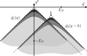
Figure F.1. Example for the integrand of $\hat{M}^{Lg}$.

We have information on the integrand only when both $q$ and $q-k$ are close to the lower mass cone, i.e. when $q$ lies in the intersection of the dark shaded regions in Figure LABEL:fig1. Outside of this so-called intersection region, however, the integrand depends on the unknown high-energy behavior of $\hat{g}_{1}$ or $\hat{g}_{2}$. Since the intersection region becomes large when $k$ comes close to the mass cone and does not depend smoothly in $k$ for $k$ on the mass cone, the contribution of the intersection region to the integral is localized in a neighborhood of and is not regular on the mass cone $\{k^{2}=0\}$. The contribution of the high-energy regions to the integral, on the other hand, is regular in $k$ and thus well-approximated by a polynomial in $k$. This qualitative argument illustrates why in Lemma F.1, $\hat{Q}$ is determined only modulo a polynomial, and why the singular behavior on the light cone (F.4) is in momentum space encoded near the lower mass cone (see Lemma F.2 and the discussion thereafter). An important conclusion from Figure F.1 is that $\hat{Q}(k)$ is in general not zero in the interior of the lower mass cone, and even the intersection region gives a contribution there. Thus for generic regularizations or for simple regularizations like mollifying with a smooth function, the supports of $\hat{Q}$ and $\hat{P}$ will have a non-empty intersection, and even the singularities of $Q$ on the light cone will contribute to the product $QP$. On the other hand, it seems possible that there are special regularizations for which the contributions from the high energy regions and the intersection region compensate each other in the integral (F.32) in such a way that $\hat{M}^{Lg}$ indeed vanishes inside the lower mass cone. We call such a regularization an optimal regularization. According to the method of variable regularization (see §LABEL:psec22), we want to keep the regularization as general as possible. Therefore, we must allow for the possibility that the regularization is optimal, and this leads to the problem of disjoint supports.

The above consideration in momentum space gives a hint on how to resolve the problem of disjoint supports. Namely, let us assume for a moment that the macroscopic function $f$ has nice decay properties at infinity. Then its Fourier transform $\hat{f}$ is a regular function. As a consequence, the convolution (F.33) mollifies $\hat{M}^{Lg}$ on the scale $l_{\mbox{\scriptsize{macro}}}^{-1}$, and the support of $\hat{Q}$ will be larger than that of $\hat{M}^{Lg}$. Clearly, $l_{\mbox{\scriptsize{macro}}}^{-1}$ is very small on the Planck scale, but since the mass shell $\{k^{2}=m^{2}\}$ and the mass cone $\{k^{2}=0\}$ come asymptotically close as the energy $|k^{0}|$ gets large, mollifying even on a small scale leads to an overlap of the supports of $\hat{Q}$ and $\hat{P}$. This is an effect which is not apparent in the expansion of Lemma F.1 because by expanding $f$ in a Taylor series around $\xi=0$, we did not use the decay properties of $f$ at infinity, and thus we did not see the smoothing in momentum space (cf. also (F.34) and (F.35)). More generally, the above “mollifying argument” shows that the supports of $\hat{Q}$ and $\hat{P}$ should overlap if we take into account the macroscopic perturbations of $P$ and $Q$ more carefully. Thus in order to solve the problem of disjoint supports, we shall now compute the product $QP$ in the case of general interaction, without assuming that $P$ or $Q$ are homogeneous. Our key result will be an expansion of the operator product around the light cone (see Theorem F.5 below).

Let us specify our assumptions on $P$ and $Q$. For $Q$ we merely assume that the weak evaluation formula (F.4) holds. For $P$, on the other hand, we work with the formulas of the light-cone expansion, which are of the general form

$$P(x,y)\;=\;\sum_{p=-1}^{\infty}g_{p}(x,y)\>T^{(p)}(x,y)\>+\>{\mbox{(smooth contributions)}}\>.$$ (F.36)

Here the $g_{p}$ are smooth functions involving the bosonic potentials and fields, and the unspecified smooth contributions are composed of the fermionic wave functions as well as the non-causal contributions to the Dirac seas (see (LABEL:1g, LABEL:fprep) and Appendix B). For clarity, we shall consider the product of $Q$ with each of the summands in (F.36) separately, i.e. we will for given $p\geq-1$ compute the product

$$Q\>R\;\;\;\;\;\;\;\;\;\;{\mbox{with}}\;\;\;\;\;\;\;\;\;\;R(x,y)\;=\;g(x,y)\>T^{(p)}(x,y)$$ (F.37)

and a smooth function $g$. To avoid confusion, we recall that in the case $p=-1$, $T^{(p)}$ is defined via a distributional derivative; more precisely, we assume in this case that $g(x,y)$ has the form $g=\xi_{j}\>f^{j}$ with smooth functions $f^{j}(x,y)$ and set similar to (LABEL:l:7)

$$g(x,y)\>T^{(-1)}(x,y)\;=\;-2\>f^{j}(x,y)\>\frac{\partial}{\partial y^{j}}T^{(0)}(x,y)\>.$$ (F.38)

For technical convenience, we assume furthermore that $g$ is a Schwartz function, $g\in{\mathcal{S}}({\mbox{\Bb R}}^{4}\times{\mbox{\Bb R}}^{4})$, but this assumption is not essential and could be relaxed by approximation (see the discussion after (F.87) below).

The contributions to $Q$ in (F.4) are supported on the light cone. Thus we can write them in the form

$$Q(x,y)\;=\;h(x,y)\>K_{a=0}(x,y)$$ (F.39)

with

$$K_{a=0}(x,y)\;=\;\frac{i}{4\pi^{2}}\>\delta(\xi^{2})\>\epsilon(\xi^{0})$$ (F.40)

and a function $h(x,y)$, which in general will have a pole at the origin $x=y$. This representation is useful because $K_{a}$ is a solution of the Klein-Gordon equation, namely in momentum space

$$K_{a}(k)\;=\;\delta(k^{2}-a)\>\epsilon(k^{0})\>,\;\;\;\;\;\;\;\;\;\;a\in[0,\infty).$$ (F.41)

In what follows, we will also need the Green’s function $S_{a}$ of the Klein-Gordon equation defined by

$$S_{a}(k)\;=\;\frac{\mbox{PP}}{k^{2}-a}\;\equiv\;\frac{1}{2}\>\lim_{\varepsilon\searrow 0}\sum_{\pm}\frac{1}{k^{2}-a\pm i\varepsilon}\>,\;\;\;\;\;\;\;\;\;\;a\in{\mbox{\Bb R}}.$$ (F.42)

As is immediately verified with contour integrals, this Green’s function is for $a>0$ causal in the sense that $S_{a}(x,y)$ vanishes for space-like $\xi$. On the contrary if $a<0$, $S_{a}(x,y)$ vanishes for time-like $\xi$. More precisely, the Green’s function can be written as

$$S_{a}(x,y)\;=\;-\frac{1}{4\pi}\>\delta(\xi^{2})\>+\>\Theta(a\xi^{2})\>\epsilon(a)\>H_{a}(x,y)\>,$$ (F.43)

where $H_{a}$ is a smooth solution of the Klein-Gordon equation with power expansion

$$H_{a}(x,y)\;=\;\frac{a}{16\pi}\>\sum_{j=0}^{\infty}\frac{(-1)^{j}}{j!\>(j+1)!}\>\frac{a^{j}\>\xi^{2j}}{4^{j}}\>.$$ (F.44)

It is convenient to also introduce the Green’s function

$$S^{\Join}_{a}\;=\;S_{a}-\Theta(a)\>H_{a}\>,$$ (F.45)

which for all $a\in{\mbox{\Bb R}}$ vanishes in time-like directions. As one sees explicitly using (F.44) and (F.43), both $H_{a}(x,y)$ and $S^{\Join}_{a}(x,y)$ are analytic in $a$ for all $a\in{\mbox{\Bb R}}$. Similarly, a short explicit calculation shows that $K_{a}(x,y)$ is analytic for $a\in[0,\infty)$. We set

$$K^{(n)}=\lim_{a\searrow 0}\left(\frac{d}{da}\right)^{n}K_{a}\>,\;\;\;\;S^{(n)}_{\Join}=\left(\frac{d}{da}\right)^{n}S^{\Join}_{a\>|\>a=0}\>,\;\;\;\;H^{(n)}=\left(\frac{d}{da}\right)^{n}H_{a\>|\>a=0}\>.$$

The following lemma gives the light-cone expansion for an operator product involving two factors $K^{(.)}$. A major difference to Lemma LABEL:l:lemma1 is that the expansion now contains unbounded line integrals; this also requires a different method of the proof.

Lemma F.3.

The operator product $K^{(l)}VK^{(r)}$ with $l,r\geq 0$ and a scalar function $V\in{\mathcal{S}}$ has the light-cone expansion

$$\;\;\;\;\;\;\;\;\;\;\;\;\;(K^{(l)}\>V\>K^{(r)})(x,y)$$ (F.46)

$$= \!\!\!\!\!\!-\frac{1}{2\pi^{2}}\>\sum_{n=0}^{\infty}\frac{1}{n!}\>\int_{0}^{1}d\alpha\>\alpha^{l}\>(1-\alpha)^{r}\>(\alpha-\alpha^{2})^{n}\>(\Box^{n}V)_{|\alpha y+(1-\alpha)x}\;H^{(l+r+n+1)}(x,y)$$

$$\!\!\!\!\!\!-\frac{1}{2\pi^{2}}\>\sum_{n=0}^{\infty}\frac{1}{n!}\>\int_{-\infty}^{\infty}d\alpha\>\alpha^{l}\>(1-\alpha)^{r}\>(\alpha-\alpha^{2})^{n}\>(\Box^{n}V)_{|\alpha y+(1-\alpha)x}\;S^{(l+r+n+1)}_{\Join}(x,y)$$

$$\!\!\!\!\!\!+({\mbox{non-causal contributions, smooth for $x\neq y$}}).$$

We point out that, exactly as in §LABEL:jsec5, we do not study the convergence of the infinite series in (F.46), which are merely a convenient notation for the approximation by the partial sums.

Proof of Lemma F.3. We first consider the operator product $K_{a}VK_{b}$ for $a,b>0$ in the case when $V$ is a plane wave, $V(x)=\exp(-iqx)$. Then in momentum space (similar to [F6, eqn (3.9)]), the operator product takes the form

$$(K_{a}\>V\>K_{b})\!\left(p+\frac{q}{2},\>p-\frac{q}{2}\right)\;=\;K_{a}\!\left(p+\frac{q}{2}\right)\>K_{b}\!\left(p-\frac{q}{2}\right)\>.$$ (F.47)

If $q^{2}<0$, we get contributions when either the two upper mass shells of the factors $K_{a}$ and $K_{b}$ intersect, or the two lower mass shells. Conversely if $q^{2}>0$, we only get cross terms between the upper and lower mass shells. Thus setting

$$u\;=\;\frac{a+b}{2}\>,\;\;\;\;\;\;\;\;\;\;v\;=\;\frac{a-b}{2}\>,$$ (F.48)

we have

$$(K_{a}\>V\>K_{b})\!\left(p+\frac{q}{2},\>p-\frac{q}{2}\right)\;=\;-\epsilon(q^{2})\>\delta\!\left(\!(p+\frac{q}{2})^{2}-a\right)\>\delta\!\left(\!(p-\frac{q}{2})^{2}-b\right)$$

$$= -\epsilon(q^{2})\>\delta\!\left(\!((p-\frac{q}{2})^{2}-b)\>+\>(2pq-2v)\right)\>\delta\!\left(\!(p-\frac{q}{2})^{2}-b\right)\;\;\;\;\;\;\;\;\;\;$$

$$= -\epsilon(q^{2})\>\delta(2pq-2v)\>\delta\!\left(p^{2}-pq+\frac{q^{2}}{4}-b\right)$$

$$= -\frac{1}{2}\>\epsilon(q^{2})\>\delta(pq-v)\>\delta\!\left(p^{2}+\frac{q^{2}}{4}-u\right).$$

Hence we can write our operator product as

$$K_{a}\>V\>K_{b}\;=\;\frac{d}{du}A_{uv}$$ (F.49)

where $A_{uv}$ is the operator

$$A_{uv}\!\left(p+\frac{q}{2},\>p-\frac{q}{2}\right)\;=\;\frac{1}{2}\;\delta(pq-v)\;\Theta\!\left(q^{2}\>(p^{2}+\frac{q^{2}}{4}-u)\right).$$ (F.50)

Our strategy is to first derive an expansion for $A_{uv}$. Then we will differentiate this expansion with respect to $u$ and $v$ and take the limits $a,b\searrow 0$ to get the desired expansion for $K^{(l)}VK^{(r)}$.

The right side of (F.50) involves a product of the form $\delta(\alpha)\>\Theta(\beta)$. This product can be transformed into a line integral as follows. Consider for $\varepsilon>0$ the function

$$f_{\varepsilon}(\alpha,\beta)\;=\;\frac{1}{\pi}\>\Theta(\varepsilon\beta-\alpha^{2})\>(\varepsilon\beta-\alpha^{2})^{-\frac{1}{2}}\>.$$ (F.51)

This function is zero unless $\beta>0$ and $\alpha\in[-\sqrt{\varepsilon\beta},\sqrt{\varepsilon\beta}]$. As $\varepsilon\searrow 0$, the size of this last interval tends to zero, and so $\alpha$ is confined to a smaller and smaller neighborhood of the origin. On the other hand, the integral over $\alpha$ stays bounded in this limit; namely,

$$\int_{-\infty}^{\infty}f_{\varepsilon}(\alpha,\beta)\>d\alpha\;=\;\Theta(\beta)\;\;\;\;\;\;\;\;\;\;{\mbox{for all $\varepsilon>0$}}.$$

From this we conclude that

$$\lim_{\varepsilon\searrow 0}f_{\varepsilon}(\alpha,\beta)\;=\;\delta(\alpha)\>\Theta(\beta)$$ (F.52)

with convergence as a distribution. Moreover, the formula

$$\int_{-\infty}^{\infty}\frac{\mbox{PP}}{\tau^{2}+\gamma}\>d\tau\;=\;\pi\>\Theta(\gamma)\>\gamma^{-\frac{1}{2}}$$ (F.53)

allows one to write (F.51) as a contour integral. Putting these relations together, we obtain for $A_{uv}$,

$$\;\;\;\;\;\;\;\;\;\;\;\;\;\;\;\;\;\;\;\;A_{uv}\!\left(p+\frac{q}{2},\>p-\frac{q}{2}\right)\;\stackrel{{\scriptstyle(\ref{eq:bf},\ref{eq:bh})}}{{=}}\;\frac{1}{2}\>\lim_{\varepsilon\searrow 0}f_{\varepsilon}\!\left(pq-v,\>q^{2}\>(p^{2}+\frac{q^{2}}{4}-u)\right)$$ (F.54)

$$\stackrel{{\scriptstyle(\ref{eq:bg})}}{{=}} \!\!\!\!\!\frac{1}{2\pi}\>\lim_{\varepsilon\searrow 0}\>\frac{1}{|\varepsilon q^{2}|}\;\Theta\!\left(\frac{p^{2}+\frac{q^{2}}{4}-u}{\varepsilon q^{2}}-\frac{(pq-v)^{2}}{\varepsilon^{2}q^{4}}\right)\!\!\left(\frac{p^{2}+\frac{q^{2}}{4}-u}{\varepsilon q^{2}}-\frac{(pq-v)^{2}}{\varepsilon^{2}q^{4}}\right)^{-\frac{1}{2}}$$

$$\stackrel{{\scriptstyle(\ref{eq:bi})}}{{=}} \!\!\!\!\!\frac{\epsilon(q^{2})}{2\pi^{2}}\>\lim_{\varepsilon\searrow 0}\int_{-\infty}^{\infty}\frac{\mbox{PP}}{\displaystyle\varepsilon q^{2}\tau^{2}+p^{2}+\frac{q^{2}}{4}-u-\frac{(pq-v)^{2}}{\varepsilon q^{2}}}\;d\tau\>.$$

After shifting the integration variable according to $\tau\to\tau+(pq-v)/(\varepsilon q^{2})$, we can identify the integrand with the Green’s function (F.42),

$$A_{uv}\!\left(p+\frac{q}{2},\>p-\frac{q}{2}\right)$$ (F.55)

$$= \frac{\epsilon(q^{2})}{2\pi^{2}}\;\lim_{\varepsilon\searrow 0}\int_{-\infty}^{\infty}\frac{\mbox{PP}}{\displaystyle p^{2}+2\tau(pq-v)+\varepsilon^{2}q^{2}\tau^{2}+\frac{q^{2}}{4}-u}\;d\tau$$

$$= \frac{\epsilon(q^{2})}{2\pi^{2}}\>\lim_{\varepsilon\searrow 0}\int_{-\infty}^{\infty}S_{z(\varepsilon,\tau)}(p+\tau q)\>,$$

where $z$ is the “mass function”

$$z(\varepsilon,\tau)\;=\;u\>+\>2\tau v\>+\>(1-\varepsilon^{2})\>\tau^{2}\>q^{2}\>-\>\frac{q^{2}}{4}\>.$$

If we solve (F.45) for $S_{a}$ and substitute into (F.55), we can take the limit $\varepsilon\searrow 0$ to obtain

$$A_{uv}\!\left(p+\frac{q}{2},\>p-\frac{q}{2}\right)\;=\;\frac{\epsilon(q^{2})}{2\pi^{2}}\>\int_{-\infty}^{\infty}(S^{\Join}_{z}+\Theta(z)\>H_{z})(p+\tau q)\;d\tau$$ (F.56)

with

$$z\;\equiv\;u\>+\>2\tau v\>+\>(\tau^{2}-\frac{1}{4})\>q^{2}\>.$$ (F.57)

The calculation so far was carried out for fixed momentum $q$ of the potential. In order to describe the case of general $V\in{\mathcal{S}}$, we must integrate over $q$. Furthermore, we transform to position space by integrating over $p$ (similar to [F5, eqn (3.10)]) and obtain

$$A_{uv}(x,y)\;=\;\int\frac{d^{4}q}{(2\pi)^{4}}\>\hat{V}(q)\int\frac{d^{4}p}{(2\pi)^{4}}\>A_{uv}(p+\frac{q}{2},p-\frac{q}{2})\;e^{-ip(x-y)}\>e^{-i\>\frac{q}{2}\>(x+y)}\>,$$

where $\hat{V}$ is the Fourier transform of $V$. Substituting in (F.56) and pulling out the $\tau$-integral gives

$$A_{uv}(x,y) = \frac{1}{2\pi^{2}}\>\int_{-\infty}^{\infty}d\tau\>\int\frac{d^{4}q}{(2\pi)^{4}}\>\hat{V}(q)\>\epsilon(q^{2})\;e^{-i\>\frac{q}{2}\>(x+y)}$$

$$\hskip 28.45274pt\times\int\frac{d^{4}p}{(2\pi)^{4}}\>(S^{\Join}_{z}+\Theta(z)\>H_{z})(p+\tau q)\;e^{-ip(x-y)}\>,$$

and, after shifting the integration variable $p$ according to $p+\tau q\to p$, we can carry out the Fourier integral,

$$\int\frac{d^{4}p}{(2\pi)^{4}}\>(S^{\Join}_{z}+\Theta(z)\>H_{z})(p+\tau q)\;e^{-ip(x-y)}\;=\;e^{iq\tau(x-y)}\>(S^{\Join}_{z}+\Theta(z)\>H_{z})(x,y)\>,$$

and thus obtain

$$A_{uv}(x,y) = \frac{1}{2\pi^{2}}\>\int_{-\infty}^{\infty}d\tau\>\int\frac{d^{4}q}{(2\pi)^{4}}\>\hat{V}(q)\>\epsilon(q^{2})$$ (F.58)

$$\times\;e^{-iq((\frac{1}{2}-\tau)x+(\frac{1}{2}+\tau)y)}\>(S^{\Join}_{z}+\Theta(z)\>H_{z})(x,y)\>.$$

In this way, we have transformed the line integral, which appeared in (F.54) as a contour integral in momentum space, into an integral along the straight line $(\frac{1}{2}-\tau)x+(\frac{1}{2}+\tau)y$ through the space-time points $x$ and $y$.

The operator product $K^{(l)}VK^{(r)}$ is obtained from $A_{uv}$ by differentiating with respect to $u,v$ and setting $u=0=v$. More precisely, using (F.48) and (F.49),

$$(K^{(l)}\>V\>K^{(r)})(x,y)\;=\;\frac{1}{2^{l+r}}\left(\frac{\partial}{\partial u}+\frac{\partial}{\partial v}\right)^{l}\left(\frac{\partial}{\partial u}-\frac{\partial}{\partial v}\right)^{r}\frac{\partial}{\partial u}\left.A_{uv}\right|_{u=0=v}\>.$$ (F.59)

According to (F.57), the factors $S^{\Join}_{z}$, $\Theta(z)$, and $H_{z}$ in (F.58) depend implicitly on $u$ and $v$. Thus when substituting (F.58) into (F.59), we can carry out the partial derivatives with the sum, product, and chain rules. Let us first collect the terms for which all the derivatives act on the factors $S^{\Join}_{z}$ or $H_{z}$. This gives the contributions to $(K^{(l)}VK^{(r)})(x,y)$

$$\frac{1}{2\pi^{2}}\>\int_{-\infty}^{\infty}d\tau\>(\frac{1}{2}+\tau)^{l}\>(\frac{1}{2}-\tau)^{r}\>\int\frac{d^{4}q}{(2\pi)^{4}}\>\hat{V}(q)\>\epsilon(q^{2})\>e^{-i\>\frac{q}{2}\>(x+y)}$$

$$\hskip 28.45274pt\times\>e^{iq\tau\>(x-y)}\>(S_{z}^{\Join\>(l+r+1)}+\Theta(z)\>H_{z}^{(l+r+1)})(x,y)$$

with $z=(\tau^{2}-\frac{1}{4})\>q^{2}$. After expanding in powers of $z$ and introducing the new integration variable $\alpha=\tau+\frac{1}{2}$, we obtain

$$\frac{1}{2\pi^{2}}\>\sum_{n=0}^{\infty}\>\frac{1}{n!}\>\int_{-\infty}^{\infty}d\alpha\>\alpha^{l}\>(1-\alpha)^{r}\>(\alpha-\alpha^{2})^{n}\>\int\frac{d^{4}q}{(2\pi)^{4}}\>\epsilon(q^{2})\>(-q^{2})^{n}\>\hat{V}(q)$$ (F.60)

$$\times\>e^{-iq(\alpha y+(1-\alpha)x)}\>(S_{z}^{\Join\>(l+r+n+1)}+\Theta((\alpha^{2}-\alpha)\>q^{2})\>H_{z}^{(l+r+n+1)})(x,y)\>.\qquad$$

If $\hat{V}$ is supported outside the mass cone, ${\mbox{supp }}\hat{V}\subset\{q^{2}<0\}$, we can carry out the $q$-integral in (F.60) and obtain precisely the two series in (F.46). Conversely if $\hat{V}$ is supported inside the mass cone $\{q^{2}>0\}$, we get

$$\frac{1}{2\pi^{2}}\>\sum_{n=0}^{\infty}\frac{1}{n!}\>\int_{\mbox{\rm\scriptsize I R}\setminus[0,1]}d\alpha\>\alpha^{l}\>(1-\alpha)^{r}\>(\alpha-\alpha^{2})^{n}\>(\Box^{n}V)_{|\alpha y+(1-\alpha)x}\;H^{(l+r+n+1)}(x,y)$$

$$+\frac{1}{2\pi^{2}}\>\sum_{n=0}^{\infty}\frac{1}{n!}\>\int_{-\infty}^{\infty}d\alpha\>\alpha^{l}\>(1-\alpha)^{r}\>(\alpha-\alpha^{2})^{n}\>(\Box^{n}V)_{|\alpha y+(1-\alpha)x}\;S^{(l+r+n+1)}_{\Join}(x,y)\>.$$

This does not coincide with the series in (F.46). Using (F.45) and (F.43), the difference can be written as

$$\begin{split}\@ADDCLASS{ltx_eqn_lefteqn}$\displaystyle-\frac{1}{2\pi^{2}}\>\sum_{n=0}^{\infty}\frac{1}{n!}\int_{-\infty}^{\infty}d\alpha\;\alpha^{l}\>(1-\alpha)^{r}\>(\alpha-\alpha^{2})^{n}$\mbox{}\hfil\\ &\;\;\;\;\;\;\;\;\;\;\times(\Box^{n}V)_{|\alpha y+(1-\alpha)x}\;\epsilon(\xi^{2})\>H^{(l+r+n+1)}(x,y)\>.\;\end{split}$$ (F.61)

Since unbounded line integrals are involved, this expression is clearly non-causal. We shall now prove that (F.61) is smooth for $x\neq y$. Notice that the line integrals in (F.61) are supported on the hyperplane $\{q\>|\>q\xi=0\}$, e.g.

$$\int_{-\infty}^{\infty}V(\alpha y+(1-\alpha)x)\>d\alpha\;=\;\int\frac{d^{4}q}{(2\pi)^{4}}\>\hat{V}(q)\;2\pi\delta(q\xi)\;e^{-i\>\frac{q}{2}\>(x+y)}\>.$$ (F.62)

For time-like $\xi$, this hyperplane does not intersect the support of $\hat{V}$, and thus (F.61) vanishes identically inside the light cone. Furthermore, (F.61) is clearly smooth in the region $\{\xi^{2}<0\}$ away from the light cone. Thus it remains to show that all the partial derivatives of (F.61) vanish on the light cone. The boundary values of these partial derivatives on the light cone $\{\xi^{2}=0\}$ involve integrals of the form

$$\int_{-\infty}^{\infty}d\alpha\>\alpha^{l+k_{1}}\>(1-\alpha)^{r+k_{2}}\>(\alpha-\alpha^{2})^{n}\>(\partial^{K}\Box^{n}V)_{|\alpha y+(1-\alpha)x}\>\xi^{L}$$

with parameters $k_{1},k_{2}\geq 0$ and multi-indices $K$, $L$. Similar to (F.62), these integrals are supported on the hypersurface $\{q\>|\>q\xi\}=0$, and for $\xi$ on the light cone (and $\xi\neq 0$), this hypersurface does not intersect the support of $\hat{V}$. We conclude that (F.60) coincides with (F.46), both in the case when ${\mbox{supp }}\hat{V}\subset\{q^{2}<0\}$ and when ${\mbox{supp }}\hat{V}\subset\{q^{2}>0\}$. Linearity and an approximation argument near the light cone yield that (F.60) coincides with (F.46) for general $V\in{\mathcal{S}}$.

It remains to consider the contributions when some of the derivatives in (F.59) act on the factor $\Theta(z)$ in (F.58). The resulting expressions are of the form

$$\int\frac{d^{4}q}{(2\pi)^{4}}\>\hat{V}(q)\>e^{-i\>\frac{q}{2}\>(x+y)}\>\int_{-\infty}^{\infty}d\tau\;\epsilon(q^{2})\>\delta^{(\alpha)}(z)\>H^{(\beta)}_{z}(x,y)\>{\mathcal{P}}(\tau)\;e^{-iq\tau(y-x)}$$ (F.63)

with integers $\alpha,\beta\geq 0$ and a polynomial ${\mathcal{P}}(\tau)$. Using the formula

$$\delta(z)\;=\;\frac{1}{2\pi i}\>\lim_{\varepsilon\searrow 0}\left(\frac{1}{z-i\varepsilon}-\frac{1}{z+i\varepsilon}\right),$$

we can write the $\tau$-integral in terms of the complex integrals

$$\lim_{\varepsilon\searrow 0}\epsilon(q^{2})\>\int_{-\infty}^{\infty}d\tau\>\frac{1}{((\tau^{2}-\frac{1}{4})\>q^{2}\pm i\varepsilon)^{\alpha+1}}\>H^{(\beta)}_{z}\>{\mathcal{P}}(\tau)\>e^{-iq\tau(y-x)}\>.$$

Depending on the sign of $q(y-x)$, the integration contour can be closed either in the upper or in the lower half plane, and the residue theorem yields expressions of the form

$$\lim_{\varepsilon\searrow 0}\>\frac{1}{(q^{2}\pm i\varepsilon)^{\gamma}}\>H^{(\kappa)}(x-y)\>{\mathcal{P}}(\tau)\>e^{-iq\tau(y-x)}\;\;\;\;\;\;\;\;\;\;{\mbox{with}}\;\;\;\;\;\;\;\;\;\;\tau=\pm\frac{1}{2}$$ (F.64)

and $\gamma\leq 2\alpha+1$, $\beta\leq\kappa\leq\beta+\alpha$. These expressions are well-defined distributions, and thus the $q$-integral in (F.63) is finite. Due to the powers of $1/q^{2}$ in (F.64), the resulting contributions to the operator product $K^{(l)}VK^{(r)}$ are non-causal. Since the factor $H^{(\kappa)}$ in (F.64) is a polynomial in $\xi$ and $\hat{V}(q)$ in (F.63) has rapid decay, these contributions are also smooth.    

The above lemma can be used to derive the light-cone expansion for the operator product $K^{(l)}VT^{(r)}$.

Lemma F.4.

For $l,r\geq 0$ and $V\in{\mathcal{S}}$,

$$\;\;\;\;(K^{(l)}\>V\>T^{(r)})(x,y)$$ (F.65)

$$= \frac{1}{2\pi i}\>\sum_{n=0}^{\infty}\frac{1}{n!}\>\int_{-\infty}^{\infty}d\alpha\>\alpha^{l}\>(1-\alpha)^{r}\>(\alpha-\alpha^{2})^{n}\>(\Box^{n}V)_{|\alpha y+(1-\alpha)x}$$

$$\times\;\epsilon(y^{0}-x^{0})\>T^{(l+r+n+1)}(x,y)\>+\>({\mbox{contributions smooth for $x\neq y$}})\>.\qquad$$

Proof. Using (F.45) and the fact that $H_{a}(x,y)$ is smooth in $x$ and $y$ according to (F.44), the light-cone expansion (F.46) yields that for $p,q\geq 0$,

$$(K^{(l)}\>V\>K^{(r)})(x,y)$$ (F.66)

$$\!\!\!\!\!\!\!\!=\,-\frac{1}{2\pi^{2}}\>\sum_{n=0}^{\infty}\frac{1}{n!}\>\int_{-\infty}^{\infty}\!\!\!d\alpha\>\alpha^{l}\>(1-\alpha)^{r}\>(\alpha-\alpha^{2})^{n}\>(\Box^{n}V)_{|\alpha y+(1-\alpha)x}\;S^{(l+r+n+1)}(x,y)$$

$$+({\mbox{contributions smooth for $x\neq y$}})\>,$$

where $S^{(n)}=\lim_{a\searrow 0}S_{a}^{(n)}$. The main difference between (F.65) and (F.66) is that the factors $K^{(r)}$ and $S^{(l+r+n+1)}$ are replaced by corresponding factors $T^{(.)}$. The method of the proof is to realize these replacements by multiplying (F.66) with a suitable operator from the right.

In preparation, we rewrite the operators $S^{(.)}$ in (F.66) in terms of $K^{(.)}$ as follows. Using that multiplication in position space corresponds to convolution in momentum space, we have for $a>0$,

$$\int K_{a}(x,y)\>\epsilon(y^{0}-x^{0})\>e^{-ik\>\xi}\>d^{4}\xi$$

$$= \int_{-\infty}^{\infty}\frac{d\omega}{2\pi}\;\delta(\omega^{2}-|\vec{k}|^{2}-a)\>\epsilon(\omega)\;(-2i)\>\frac{\mbox{PP}}{k^{0}-\omega}$$

$$= \frac{1}{i\pi}\>\frac{1}{2\>|\omega|}\left.\frac{\mbox{PP}}{k^{0}-\omega}\right|_{\omega=-\sqrt{|\vec{k}|^{2}+a}}^{\omega=\sqrt{|\vec{k}|^{2}+a}}\;=\;\frac{1}{i\pi}\>\frac{\mbox{PP}}{k^{2}-a}\;=\;\frac{1}{i\pi}\>S_{a}(k)\>,$$

and thus

$$S_{a}(x,y)\;=\;i\pi\>K_{a}(x,y)\;\epsilon(y^{0}-x^{0})\>.$$

We differentiate with respect to $a$ and let $a\searrow 0$ to obtain

$$S^{(n)}(x,y)\;=\;i\pi\>K^{(n)}(x,y)\;\epsilon(y^{0}-x^{0})\>.$$

Substituting into (F.66) gives

$$(K^{(l)}\>V\>K^{(r)})(x,y)\;=\;({\mbox{contributions smooth for $x\neq y$}})$$ (F.67)

$$\>+\>\frac{1}{2\pi i}\>\sum_{n=0}^{\infty}\frac{1}{n!}\int_{-\infty}^{\infty}d\alpha\>\epsilon(y^{0}-x^{0})\>\alpha^{l}\>(1-\alpha)^{r}\>(\alpha-\alpha^{2})^{n}$$

$$\hskip 99.58464pt\times\>(\Box^{n}V)_{|\alpha y+(1-\alpha)x}\;K^{(l+r+n+1)}(x,y)\>.$$

The operator $T_{a}$, $a\geq 0$, is obtained from $K_{a}$ by projecting on the negative-energy states, more precisely

$$T_{a}\;=\;K_{a}\>\chi\>,$$ (F.68)

where $\chi$ is the multiplication operator in momentum space

$$\chi(k)\;=\;-\Theta(-k^{0})\>.$$

In position space, $\chi$ has the kernel

$$\chi(x,y)\;=\;\int\frac{d^{4}k}{(2\pi)^{4}}\>\chi(k)\>e^{-ik(x-y)}\;=\;-\frac{1}{2\pi i}\>\lim_{\varepsilon\searrow 0}\frac{1}{y^{0}-x^{0}-i\varepsilon}\>\delta^{3}(\vec{y}-\vec{x})\>.$$ (F.69)

If $a$ is positive, the mass shell $\{k^{2}=a\}$ does not intersect the hyperplane $\{k^{0}=0\}$ where $\chi$ is not smooth, and thus we may differentiate (F.68) with respect to $a$ to obtain

$$T_{a}^{(n)}\;=\;K_{a}^{(n)}\>\chi\>,\;\;\;\;\;\;\;\;\;\;a>0.$$ (F.70)

However, difficulties arise in (F.70) in the limit $a\searrow 0$. Namely, the limit of the left side exist only after “regularizing” $T_{a}^{(n)}$ by subtracting a polynomial in $(y-x)$ (see (LABEL:Tadef, LABEL:Tldef). On the right side, the problem is that $K^{(n)}(x,y)$ behaves polynomially at timelike infinity, whereas $\chi(x,y)$ decays for large $(y^{0}-x^{0})$ only as $(y^{0}-x^{0})^{-1}$, and so the product $K^{(n)}\chi$ does not exist. To cure this problem, we insert into (F.69) an exponentially decaying factor by introducing for $\kappa>0$ the kernel

$$\chi_{\kappa}(x,y)\;=\;-\frac{1}{2\pi i}\>\lim_{\varepsilon\searrow 0}\frac{e^{-\kappa\>|y^{0}-x^{0}|}}{y^{0}-x^{0}-i\varepsilon}\>\delta^{3}(\vec{y}-\vec{x})\>.$$ (F.71)

The exponential factor changes the product with $K_{a}^{(n)}$ only by a contribution smooth in $y-x$, and thus

$$T_{a}^{(n)}(x,y)+{\mbox{(smooth contributions)}}$$

$$= T_{a}^{(n)}(x,y)\;=\;(K_{a}^{(n)}\>\chi)(x,y)\;=\;(K_{a}^{(n)}\>\chi_{\kappa})(x,y)+{\mbox{(smooth contributions)}}\>.$$

The very left and right of this equation converge for $a\searrow 0$, and we conclude that

$$(K^{(n)}\>\chi_{\kappa})(x,y)\;=\;T^{(n)}(x,y)\>+\>{\mbox{(smooth contributions)}}.$$ (F.72)

We multiply the operator product on the left of (F.67) by the operator $\chi_{\kappa}$. Applying (F.72) and using that multiplying by a smooth operator gives something smooth, we get

$$(K^{(l)}\>V\>K^{(r)}\>\chi_{\kappa})(x,y)\;=\;(K^{(l)}\>V\>T^{(r)})(x,y)\>+\>{\mbox{(smooth contributions)}}.$$ (F.73)

It remains to show that multiplying the right side of (F.67) by the operator $\chi_{\kappa}$ gives the right side of (F.65). When we multiply the summands on the right side of (F.67) by $\chi_{\kappa}$, we get according to (F.71) a convolution in the time coordinate of the form

$$\lim_{\varepsilon\searrow 0}\int_{-\infty}^{\infty}d\tau\>\frac{e^{-\kappa\>|\tau|}}{\tau-i\varepsilon}\>F(x;y^{0}-\tau,\vec{y})\>K^{(l+r+n+1)}(x;y^{0}-\tau,\vec{y})\>.$$ (F.74)

Here the function $F$ stands for the line integral in (F.67); it is smooth unless $y^{0}-\tau=x^{0}$. We write the convolution integral (F.73) as

$$\lim_{\varepsilon\searrow 0}\int_{-\infty}^{\infty}d\tau\>e^{-\kappa\>|\tau|}\>\frac{F(x;y^{0}-\tau,\vec{y})-F(x,y)}{\tau-i\varepsilon}\>K^{(l+r+n+1)}(x;y^{0}-\tau,\vec{y})$$ (F.75)

$$+F(x,y)\;\lim_{\varepsilon\searrow 0}\int_{-\infty}^{\infty}d\tau\>\frac{e^{-\kappa\>|\tau|}}{\tau-i\varepsilon}\>K^{(l+r+n+1)}(x;y^{0}-\tau,\vec{y})\>.$$ (F.76)

The term (F.76) can be written as $F(x,y)\>(K^{(l+r+n+1)}\>\chi_{\kappa})(x,y)$, and applying (F.72) gives precisely the summands on the right side of (F.65). Let us prove that (F.75) is smooth for $x\neq y$. Thus assume that $x\neq y$. Our above construction is Lorentz invariant in the sense that we may introduce the operator $\chi_{\kappa}$ in any reference frame, without influence on our operator products. Thus we can choose the reference frame such that $\vec{x}\neq\vec{y}$. The $\tau$-integral in (F.75) can be regarded as an integral along the straight line $\{(y^{0}-\tau,\vec{y})\}$. Since $\vec{x}\neq\vec{y}$, this straight line does not intersect the point $x$. Due to causality of $K^{(.)}$, the integrand vanishes unless $|(y^{0}-\tau)-x^{0}|\geq|\vec{y}-\vec{x}|$. Thus if $\xi$ is spacelike, i.e. $|y^{0}-x^{0}|<|\vec{y}-\vec{x}|$, the integrand vanishes in a neighborhood of $\tau=0$, and as a consequence the integral (F.75) is smooth in $x$ and $y$. On the other hand if $\xi$ lies inside the cone $|y^{0}-x^{0}|>\frac{1}{2}\>|\vec{y}-\vec{x}|$, the straight line $\{(y^{0}-\tau,\vec{y})\}$ does for small enough $\tau$ not intersect the hyperplane $\{z\>|\>z^{0}=x^{0}\}$ where $F$ is not smooth. Thus the function $F(x;y^{0}-\tau,\vec{y})$ is smooth in a neighborhood of $\tau=0$, and the mean value theorem yields that the bracket in (F.75) is smooth. This implies that (F.75) is again smooth in $x$ and $y$.

It remains to show that multiplying the contributions smooth for $x\neq y$, which are not specified in (F.67), by the operator $\chi_{\kappa}$, gives terms which are again smooth for $x\neq y$. Again using Lorentz invariance, we can choose a reference frame such that $\vec{x}\neq\vec{y}$. Then multiplying by $\chi_{\kappa}$ yields a convolution along the straight line $\{(y^{0}-\tau,\vec{y})\}$, and this line integral does not intersect the point $x$. In this way, we can avoid integrating across the origin where the contributions in (F.67) may be singular. We get a convolution of $\chi_{\kappa}$ with a smooth function, and this is clearly finite and depends smoothly on $x$ and $y$.    

After these preliminaries, we are ready to compute the operator product $QR$ in an expansion around the light cone. For the statement of the result, we need to analytically extend $h_{J}(\Omega)$ in (F.4) from a function on $S^{2}$ to a function on Minkowski space and also regularize it at the origin: As a smooth function on $S^{2}$, $h_{J}$ can be expanded in spherical harmonics. Since the spherical harmonics are the boundary values on $S^{2}$ of the harmonic polynomials on ${\mbox{\Bb R}}^{3}$, we have the unique expansion

$$h_{J}(\vec{x})\;=\;\sum_{n=0}^{\infty}\left.{\mathcal{P}}_{n}(\vec{x})\right|_{\vec{x}\in S^{2}}\>,$$ (F.77)

where ${\mathcal{P}}_{n}(\vec{x})$ are suitable harmonic polynomials of degree $n$. The smoothness of $h_{J}$ implies that the summands in (F.77) decay in $n$ faster than any polynomial. As a consequence, the series in (F.77) converges absolutely for any $\vec{x}\in{\mbox{\Bb R}}^{3}$, and we can even extend $h_{J}(\vec{x})$ to a unique function on ${\mbox{\Bb C}}^{3}$. For $\varepsilon>0$, we define the regularization $h_{J}^{\varepsilon}$ of $h_{J}$ by

$$h_{J}^{\varepsilon}(\xi)\;=\;h_{J}\!\left(\frac{\vec{\xi}}{\xi^{0}-i\varepsilon}\right)\>.$$ (F.78)

Theorem F.5.

Assume that the operator $Q$ satisfies the weak evaluation formula (F.4). Then the operator product $QR$ with $R$ according to (F.37) with $p\geq-1$ and $g\in{\mathcal{S}}({\mbox{\Bb R}}^{4}\times{\mbox{\Bb R}}^{4})$ has the expansion

$$\hskip 31.2982pt(Q\>R)(x,y)\;=\;\sum_{L=2}^{L_{\mbox{\tiny{max}}}}\>\sum_{g=0}^{g_{\mbox{\tiny{max}}}}\log^{g}(E_{P})\>E_{P}^{L-1}\>\sum_{J}$$ (F.81)

$$\times\>(-2\pi)\sum_{n=0}^{\infty}\lim_{\varepsilon\searrow 0}\int_{-\infty}^{\infty}\!\!\!\!d\alpha\>(1-\alpha)^{p}\>(\alpha-\alpha^{2})^{n}\>\Box_{z}^{n}\!\left(\frac{h_{J}^{\varepsilon}(\zeta)\>\zeta^{J}}{(\zeta^{0}-i\varepsilon)^{L-1}}\>g(z,y)\right)_{|z=\alpha y+(1-\alpha)x}$$

$$\times\>\epsilon(y^{0}-x^{0})\;T^{(p+n+1)}(x,y)\;{\mbox{ mod }}\;{\mathcal{P}}^{L-|J|-3}(\partial_{x})\>R(x,y)\>+\>o(E_{P})$$

$$+\>{\mbox{(contributions smooth for $x\neq y$)}}\>+\>{\mbox{(higher orders in $(l_{\mbox{\scriptsize{macro}}}E_{P})^{-1}$)}}$$

with $\zeta\equiv z-x$.

Proof. We first consider the case $p\geq 0$. We fix two space-time points $x_{0}$, $y_{0}$ and set

$$Q(\xi)\;:=\;Q(x_{0},x_{0}+\xi)\>,\;\;\;\;\;\;\;\;\;\;R(\xi)\;:=\;R(y_{0}-\xi,y_{0})\>.$$

We regard $Q(\xi)$ and $R(\xi)$ as the integral kernels of corresponding homogeneous operators, which with slight abuse of notation we denote again by $Q$ and $R$. Then in momentum space (F.11), the operator $Q$ has the expansion of Lemma F.1 and Lemma F.2. Let us compute the product $Q^{Lg}_{J}R$. According to its construction in Lemma F.1, $Q^{Lg}_{J}(\xi)$ behaves for $\xi\neq 0$ like

$$Q^{Lg}_{J}(\xi)\;=\;\delta(\xi^{2})\>\epsilon(\xi^{0})\>t^{-L+1}\;h_{J}(\check{\xi})\>\xi^{J}\>,$$

and furthermore its Fourier transform $\hat{Q}^{Lg}_{J}(k)$ vanishes inside the lower mass cone (cf. Lemma F.2). The distribution

$$\lim_{\varepsilon\searrow 0}K^{(0)}(x,y)\left[-4\pi^{2}i\>(y^{0}-x^{0}-i\varepsilon)^{-L+1}\>h_{J}(\check{\xi})\>\xi^{J}\right]$$ (F.82)

has these two properties, as one sees immediately from (F.40) and when computing the Fourier transform of (F.82) with contour integrals. Indeed, a short calculation shows that (F.82) even coincides with $Q^{Lg}_{J}(\xi)$.

We introduce for $\varepsilon>0$ the potential

$$V_{\varepsilon}(z)\;=\;-4\pi^{2}i\>(z^{0}-x_{0}^{0}-i\varepsilon)^{-L+1}\>h_{J}^{\varepsilon}(z-x_{0})\;(z-x_{0})^{J}\>g(z,y_{0})\>,$$

where $h^{\varepsilon}_{J}$ is the regularization of $h_{J}$ (F.78). This potential is a Schwartz function, and thus Lemma F.4 yields that

$$\;\;\;\;\;(K^{(0)}\>V^{\varepsilon}\>T^{(p)})(x,y)$$ (F.83)

$$=\;\frac{1}{2\pi i}\>\sum_{n=0}^{\infty}\frac{1}{n!}\;\int_{-\infty}^{\infty}d\alpha\>(1-\alpha)^{p}\>(\alpha-\alpha^{2})^{n}\>(\Box^{n}V_{\varepsilon})_{|\alpha y+(1-\alpha)x}$$

$$\;\;\;\;\;\times\>\epsilon(y^{0}-x^{0})\;T^{(p+n+1)}(x,y)\>+\>({\mbox{contributions smooth for $x\neq y$}})\>.$$

We now set $x=x_{0}$, $y=y_{0}$ and take the limit $\varepsilon\searrow 0$. On the left side of (F.83), we can use that $(\ref{eq:bbm})=Q^{Lg}_{J}(\xi)$ to obtain the operator product $(Q^{Lg}_{J}R)(x_{0},y_{0})$. Furthermore, due to our regularization of $h_{J}^{\varepsilon}$, the factors $(\Box^{n}V_{\varepsilon})(z)$ on the right side of (F.83) are of the form smooth function times $(z^{0}-x^{0}-i\varepsilon)^{-l}$, and thus the limit $\varepsilon\searrow 0$ exists in each line integral in (F.83). We conclude that $(Q^{Lg}_{J}R)(x,y)$ coincides precisely with the series (F.81). Since in (F.83) we integrate across the origin, the higher orders in $((r+|t|)E_{P})^{-1}$ in (F.4) (or equivalently the higher orders in $k/E_{P}$ in (F.16)) yield contributions of higher order in $(l_{\mbox{\scriptsize{macro}}}E_{P})^{-1}$. Finally, calculating modulo polynomials in (F.17) means in position space that $Q(x,y)$ is determined only modulo partial derivatives of $\delta^{4}(x-y)$, and this gives rise to the term ${\mbox{ mod }}{\mathcal{P}}^{L-|J|-3}(\partial_{x})\>R(x,y)$ in (F.81). This concludes the derivation of (F.81–F.81) in the case $p\geq 0$.

In the above derivation we neglected the contributions smooth for $x\neq y$, which are not specified in (F.83), implicitly assuming that they remain smooth in the limit $\varepsilon\searrow 0$. This is justified as follows. As $\varepsilon\searrow 0$, the potential $V_{\varepsilon}(z)$ becomes singular only at $z=x_{0}$. Thus if the contributions smooth for $x\neq y$ in (F.83) had a non-smooth limit, the resulting non-smooth contributions to $(Q^{Lg}_{J}R)(x_{0},y_{0})$ would depend on $g(z,y_{0})$ and its partial derivatives only at $z=x_{0}$; i.e. they would be of the form

$$\partial^{J}_{x_{0}}g(x_{0},y_{0})\>W_{J}(x_{0},y_{0})\>,$$ (F.84)

where $W_{J}$ are distributions independent of $g$. Suppose that the Fourier transform $\hat{g}$ of $g(x_{0}+.,y_{0})$ is supported inside the upper mass shell $\{k\>|\>k^{2}>0,k^{0}>0\}$. Then due to our $(-i\varepsilon)$-regularization, also the support of $\hat{V}_{\varepsilon}$ is inside the upper mass shell. As a consequence, the Fourier transforms of the distributions $K^{(0)}(x_{0},.)$ and $(V_{\varepsilon}T^{{\mbox{\scriptsize{reg}}}\>(p)})(.,y_{0})$ have disjoint supports, and the left side of (F.83) is zero. Furthermore for $\xi$ close to the light cone, the unbounded line integrals in (F.83) vanish (notice that they are supported on the hypersurface $\{k\>|\>k\xi=0\}$). We conclude that if $\hat{g}$ is supported inside the upper mass shell, then the contributions smooth for $x\neq y$ in (F.83) are zero. Taking the limit $\varepsilon\searrow 0$ yields that the contributions (F.84) vanish if $\hat{g}$ is supported inside the upper mass shell, i.e.

$$\int d^{4}k\;k^{J}\>\hat{g}(k)\;W_{J}(x_{0},y_{0})\;=\;0$$ (F.85)

for all $\hat{g}$ with ${\mbox{supp }}\hat{g}\subset\{k\>|\>k^{2}=0,k^{0}>0\}$. Since the polynomials restricted to the upper mass cone are linearly independent, (F.85) implies that the contributions (F.84) are all identically zero.

The extension to the case $p=-1$ follows exactly as in [F6, Lemma 2.2]: We pull one derivative out of the operator product,

$$\int d^{4}z\>Q(x_{0},z)\>g(z,y_{0})\>T^{(-1)}(z,y)$$

$$\stackrel{{\scriptstyle(\ref{eq:bC})}}{{=}} -2\>\frac{\partial}{\partial y^{j}}\int d^{4}z\>Q(x_{0},z)\>f^{j}(z,y_{0})\>T^{(0)}(z,y)_{|y=y_{0}}\>,$$

substitute for the integral the expansion (F.81–F.81) for $p=0$, and differentiate through.    

The above theorem gives the clue for understanding the operator product $QP$ as well as the commutator $[P,Q]$, as we shall now explain. Using that the product of $Q$ with a smooth operator is smooth, we can write the operator product $QP$ according to (F.36) in the form

$$(Q\>P)(x,y)\;=\;\sum_{p=-1}^{\infty}(Q\>P^{p})(x,y)\>+\>{\mbox{(smooth contributions)}}$$ (F.86)

with

$$P^{p}(x,y)\;=\;g_{p}(x,y)\>T^{(p)}(x,y)\>.$$ (F.87)

The summands in (F.86) are precisely of the form considered in Theorem F.5, with the only exception that the functions $g_{p}$ in (F.87) in general have no rapid decay at infinity. Fortunately, the behavior of the functions $g_{p}$ at infinity is of no relevance to us, and we can apply Theorem F.5 to each summand in (F.86) using the following approximation argument. For fixed $x$ and $y$, we choose a Schwartz function $\eta$ which is identically equal to one on a compact set $K\ni x,y$. Then the function $(g_{p}\eta)$ has rapid decay at infinity, and Theorem F.5 applies to the operator product (F.37) with $g:=g_{p}\eta$. In the discussion below leading to Corollary F.6, the function $g(z)$ enters only for $z$ in a neighborhood of $x$ and $y$. In this neighborhood, $g$ and $g_{p}$ coincide, and thus the dependence on $\eta$ drops out. This shows that the behavior of the function $g_{p}$ at infinity is indeed of no importance for Corollary F.6 below.

Let us briefly discuss the expansion (F.81–F.81). First of all, we point out that we calculate modulo terms of the form $\partial_{x}^{K}R(x,y)$ with $|K|\leq L-|J|-3$. This corresponds to the fact that we have no information on the behavior of $Q$ near the origin. For generic regularizations or simple regularizations like a cutoff in momentum space, the terms $\partial_{x}^{K}R(x,y)$ will not be zero. Thus in this case, the operator product $QR$ does not vanish, even when we take for $R$ a Dirac sea of the vacuum; this is in agreement with our consideration in momentum space after (F.35). However, the situation is much different if we assume that we have a regularization where the terms $\partial^{K}_{x}R(x,y)$ all vanish. Namely, if we then take for $R$ a Dirac sea of the vacuum, for example

$$R(x,y)\;=\;\frac{i}{2}\>\xi\mbox{ $/$}\>T^{(-1)}(x,y)\>,$$

the integrand of the line integral in (F.81) is a rational function with poles in the upper half plane, and $QR$ is zero (up to the contributions not specified in Theorem F.5). This corresponds to our observation made after (F.28) that the poles of $Q$ cannot be detected when testing with solutions of the free Dirac equation. The regularizations for which the terms $\partial^{K}_{x}R(x,y)$ vanish are just the optimal regularizations introduced after (F.35). The main advantage compared to our earlier consideration in momentum space after (F.35) is that the expansion (F.81–F.81) tells how the macroscopic perturbations of $P$ and $Q$ effect the operator product. In particular one sees that, when taking into account the macroscopic perturbations, the operator product $QP$ does in general not vanish (even for optimal regularizations), and thus the problem of disjoint supports disappears.

In an interacting system, the factor $g(z,y)$ in (F.81) is composed of the bosonic potentials and fields. Thus in the generic situation, the line integrals in (F.81) will vanish only if the operator $Q$ is identically zero. In order to make this argument clearer, it is useful not to think of $P$ as a fixed object, but to consider small dynamic perturbations of $P$. More precisely, we consider perturbations of $P$ induced by perturbations of the bosonic potentials of our physical system. In order not to disturb the Euler-Lagrange equations, these perturbations must not be arbitrary, but should satisfy the physical equations; a typical example are perturbations by an electromagnetic wave. Thus we consider variations of our system by small, physically admissible perturbations of $P$ and study the effect on the operator product $QP$. We refer to this procedure for analyzing the operator product that we test with physical perturbations of $P$. Clearly, the requirement that the perturbation should satisfy the physical equations is a strong restriction (in particular, such perturbations are not dense in the $L^{2}$ topology). The reason why it is nevertheless a reasonable concept to use physical perturbations for testing is that these perturbations enter into (F.81) only along the one-dimensional line $\{\lambda y+(1-\lambda)x\}$. In the example of the perturbation by an electromagnetic wave, the electromagnetic field appears in the function $g$ in (F.81), and by changing the location and amplitude of the wave, we can completely determine the function $h_{J}(\Omega)$ as well as the order $L-|J|-1$ of the pole of the integrand at the origin. Notice furthermore that the summands in (F.81) scale in the Planck energy exactly as the corresponding summands in the expansion (F.4). We conclude that by testing the operator product $QP$ with physical perturbations of $P$, we can reconstruct the weak evaluation formula (F.4) completely.

Next, it is instructive to consider the behavior of the summands in (F.81) as $y-x$ gets small. If $y-x$ is scaled like $(y-x)\to\lambda\>(y-x)$ with $\lambda>0$, the variable transformation $\alpha\to\lambda^{-1}\alpha$ shows that as $\lambda\searrow 0$, the line integral blows up like $\lambda^{-(2n+p+1)}$. On the other hand, the factor $T^{(p+n+1)}$ goes to zero like $\lambda^{2n+2p}$ in this limit. Thus each summand in (F.81) scales like $\lambda^{-1+p}$. It is remarkable that, no matter how large the order of the pole of $Q$ at the origin is, the operator product $QP$ has at the origin a pole of at most the order one. The reason is that in (F.81), we integrate over the pole of $Q$, and this regularizes the singularity at the origin. Since a pole of order one is integrable in three space dimensions, we do not need to study the operator product $(QP)(x,y)$ at the origin $x=y$. According to the light-cone expansion of Theorem F.5, the information contained in the weak evaluation formula (F.4) is retrieved in the operator product $QP$ by considering the singularities on the light cone away from the origin.

The expansion of Theorem F.5 immediately allows us to study also the commutator $[P,Q]$. Namely, by taking the adjoint, $(QR)(x,y)^{*}=(RQ)(y,x)$, the formula (F.81–F.81) applies to the operator product $PQ$ as well, and we can take the difference $[P,Q]=PQ-QP$. The key observation is that in the product $(QR)(x,y)$, the pole of $Q$ at the origin appears in (F.81) together with the factor $g(z,y)$ and $z\approx x$, whereas in the product $(RQ)(x,y)$, this pole is multiplied by $g(x,z)$ and $z\approx y$. Thus when testing $[P,Q](x,y)$ with perturbations of $P$, one can distinguish between the contributions from $PQ$ and $QP$ by considering perturbations which are localized near $y$ and $x$, respectively.

These results are summarized as follows.

Corollary F.6.

To every order in $E_{P}$, the poles of $Q(x,y)$ at the origin $x=y$ can be detected in the commutator $[P,Q]$ by testing with physical perturbations of $P$.

We close with a general comment on the significance of the constructions in this appendix. Due to the problem of disjoint supports, we could make sense out of the commutator $[P,Q]$ only after taking into account the macroscopic perturbations of $P$ and $Q$. As a consequence, the relevant contributions to the commutator $[P,Q]$ are by several orders of $(l_{\mbox{\scriptsize{macro}}}E_{P})^{-1}$ smaller than expected from a simple scaling argument. This can be interpreted that the causal structure of Minkowski space and the structure of the Dirac seas, which are the underlying reason for the problem of disjoint supports, have a tendency to making the commutator $[P,Q]$ small. In this way, the causal structure and the structure of the Dirac seas seem to correspond nicely to Euler-Lagrange equations of the form $[P,Q]=0$.

Appendix G Perturbation Calculation for the Spectral Decomposition of $P(x,y)\>P(y,x)$

In this appendix we shall develop a convenient method for analyzing the eigenvalues and spectral projectors of the matrix $A_{xy}\equiv P(x,y)\>P(y,x)$ and compute all contributions to the eigenvalues needed for the derivation of the effective gauge group in Chapter LABEL:esec4. Our strategy is as follows. We decompose the fermionic projector as

$$P\;=\;P_{0}\>+\>\Delta P$$

with $P_{0}$ according to (LABEL:e:3d). This gives rise to the decomposition of $A$

$$A\;=\;A_{0}\>+\>\Delta A\\$$ (G.1)

with

$$A_{0} = P_{0}(x,y)\>P_{0}(y,x)$$ (G.2)

$$\Delta A = \Delta P(x,y)\>P_{0}(y,x)\>+\>P_{0}(x,y)\>\Delta P(y,x)\>+\>\Delta P(x,y)\>\Delta P(y,x)\>.$$ (G.3)

The eigenvalues and spectral projectors of $A_{0}$ were computed explicitly in Chapter LABEL:esec3, see (LABEL:e:3spec, LABEL:e:3k). On the light cone, $P_{0}(x,y)$ has singularities of order ${\mathcal{O}}((y-x)^{-4})$, whereas $\Delta P(x,y)={\mathcal{O}}((y-x)^{-2})$. Likewise, $\Delta A$ is compared to $A_{0}$ of lower degree on the light cone. For this reason, $\Delta A$ can be treated perturbatively in the sense that the eigenvalues and spectral projectors of $A$ can be expressed to any given degree on the light cone by a finite order perturbation calculation. Apart from the purely computational aspects, the main difficulty is that $A_{0}$ may have degenerate eigenvalues, and in this case we need to carefully analyze whether the degeneracy is removed by the perturbation. Our method is to first compute projectors on invariant subspaces of $A$ (§G.1). Analyzing the perturbation on these invariant subspaces will then give the spectral decomposition of $A$ (§G.4).

G.1. Perturbation of Invariant Subspaces

We write the spectral decomposition of $A_{0}$ as

$$A_{0}\;=\;\sum_{k=1}^{K}\lambda_{k}\>F_{k}$$

with distinct eigenvalues $\lambda_{k}$ and corresponding spectral projectors $F_{k}$. As in §LABEL:esec21 we use the convention $\lambda_{1}=0$. Clearly, the $F_{k}$ are the sum of the spectral projectors counting multiplicities,

$$F_{k}\;=\;\sum_{n,c,s{\mbox{\scriptsize{ with }}}\lambda_{ncs}=\lambda_{k}}F_{ncs}$$ (G.4)

with $\lambda_{ncs}$ and $F_{ncs}$ according to (LABEL:e:3k). Since the perturbation $\Delta A$ will in general split up the degenerate eigenvalues, we cannot expect that by perturbing $F_{k}$ we obtain spectral projectors of the matrix $A$. But we can form projectors $G_{k}$ on the space spanned by all eigenvectors of $A$ whose eigenvalues are sufficiently close to $\lambda_{k}$. The $G_{k}$ are most conveniently introduced using contour integrals. We choose $\varepsilon>0$ such that

$$|\lambda_{i}-\lambda_{j}|\;<\;2\varepsilon\;\;\;\;\;\;\;\;\;\;{\mbox{for all $i,j=1,\ldots,K$ and $i\neq j$}}.$$

Then we set

$$G_{k}\;=\;\frac{1}{2\pi i}\oint_{|z-\lambda_{k}|=\varepsilon}(z-A)^{-1}\>dz\>,$$ (G.5)

The Cauchy integral formula shows that $G_{k}$ is indeed a projector on the desired subspace.

The integral formula (G.5) is very useful for a perturbation expansion. To this end, we substitute (G.1) into (G.5) and compute the inverse with the Neumann series,

$$G_{k} = \frac{1}{2\pi i}\oint_{|z-\lambda_{k}|=\varepsilon}(z-A_{0}-\Delta A)^{-1}\>dz$$

$$= \frac{1}{2\pi i}\oint_{|z-\lambda_{k}|=\varepsilon}\left(\mbox{\rm 1 1}-(z-A_{0})^{-1}\>\Delta A\right)^{-1}\>(z-A_{0})^{-1}\>dz$$

$$= \frac{1}{2\pi i}\oint_{|z-\lambda_{k}|=\varepsilon}\sum_{n=0}^{\infty}\left((z-A_{0})^{-1}\>\Delta A\right)^{n}\>(z-A_{0})^{-1}\>dz\>.$$

Interchanging the integral with the infinite sum gives the perturbation expansion,

$$G_{k}\;=\;\sum_{n=0}^{\infty}\>\frac{1}{2\pi i}\oint_{|z-\lambda_{k}|=\varepsilon}\left((z-A_{0})^{-1}\>\Delta A\right)^{n}\>(z-A_{0})^{-1}\>dz\>,$$ (G.6)

where $n$ is the order in perturbation theory. After substituting in the spectral representation for $(z-A_{0})^{-1}$,

$$(z-A_{0})^{-1}\;=\;\sum_{l=1}^{K}\frac{F_{l}}{z-\lambda_{l}}\>,$$ (G.7)

the contour integral in (G.6) can be carried out with residues. For example, we obtain to second order,

$$G_{k}\;=\;F_{k}\>+\>\sum_{l\neq k}\frac{1}{\lambda_{k}-\lambda_{l}}\left(F_{k}\>\Delta A\>F_{l}\>+\>F_{l}\>\Delta A\>F_{k}\right)\>+\>{\mathcal{O}}((\Delta A)^{3})$$ (G.8)

$$+\sum_{l,m\neq k}\frac{1}{(\lambda_{k}-\lambda_{l})(\lambda_{k}-\lambda_{m})}$$

$$\hskip 42.67912pt\times\left(F_{k}\>\Delta A\>F_{l}\>\Delta A\>F_{m}+F_{l}\>\Delta A\>F_{k}\>\Delta A\>F_{m}+F_{l}\>\Delta A\>F_{m}\>\Delta A\>F_{k}\right)$$

$$-\sum_{l\neq k}\frac{1}{(\lambda_{k}-\lambda_{l})^{2}}$$

$$\hskip 42.67912pt\times\left(F_{k}\>\Delta A\>F_{k}\>\Delta A\>F_{l}+F_{k}\>\Delta A\>F_{l}\>\Delta A\>F_{k}+F_{l}\>\Delta A\>F_{k}\>\Delta A\>F_{k}\right).\;\;\;\;\;\;\;\;\;\;$$

To order $n>2$, the corresponding formulas are clearly more complicated, but even then they involve matrix products which are all of the form

$$F_{k_{1}}\>\Delta A\>F_{k_{2}}\>\Delta A\>\cdots\>F_{k_{n}}\>\Delta A\>F_{k_{n+1}}\>.$$ (G.9)

Substituting in (G.4) and expanding, we can just as well consider matrix products of the form (G.9) with the factors $F_{k}$ replaced by $F_{ncs}$. Furthermore, for the computation of the eigenvalues we need to take the expectation values of $G_{k}$ with certain matrix elements of $\Delta A$. This leads us to traces of matrix products of the form

$$\mbox{\rm{Tr}\/}\left(F_{n_{1}c_{1}s_{1}}\>\Delta A_{1}\>F_{n_{2}c_{2}s_{2}}\>\Delta A_{2}\>\cdots\>F_{n_{l}c_{l}s_{l}}\>\Delta A_{l}\right)$$ (G.10)

with $l=n+1$. We refer to a trace of the form (G.10) as a matrix trace. Our first task is to develop an efficient method for computing matrix traces (§G.2 and §G.3); after that we will proceed with the calculation of the eigenvalues of $A$ (§G.4).

G.2. Factorization of Matrix Traces

If one attempts to calculate a matrix trace (G.10) directly by substituting in the formulas of the light-cone expansion, the resulting expressions become so complicated and involve so many Dirac matrices that they are almost impossible to handle. We shall now simplify the situation by giving a procedure which allows us to factor matrix traces into a product of so-called elementary traces, which are much easier to compute. According to (G.3), we can assume that each factor $\Delta A_{j}$ in (G.10) is the product of a contribution to $P(x,y)$ with a contribution to $P(y,x)$. Denoting the contributions to $P(x,y)$ by $B_{j}$ and using that the corresponding contributions to $P(y,x)$ are obtained by taking the adjoint with respect to the spin scalar product, we can write each $\Delta A_{j}$ in the form

$$\Delta A_{j}\;=\;B_{j_{1}}\>B^{*}_{j_{2}}\>.$$

Inserting the completeness relation

$$\sum_{ncs}F_{ncs}\;=\;\mbox{\rm 1 1}$$

and expanding gives for (G.10) a sum of terms of the form

$$\mbox{\rm{Tr}\/}\left(F_{n_{1}c_{1}s_{1}}\>B_{1}\>F_{n_{2}c_{2}s_{2}}\>B_{2}^{*}\>\cdots\>F_{n_{k-1}c_{k-1}s_{k-1}}\>B_{k-1}\>F_{n_{k}c_{k}s_{k}}\>B_{k}^{*}\right)$$ (G.11)

with indices $(n_{j},s_{j},c_{j})$ (which are in general different from those in (G.10)) and $k=2l$.

In order to handle the sector indices in (G.11), we introduce operators $K_{n_{1},n_{2}}$ which act on the sector index and map sector $n_{2}$ to sector $n_{1}$, i.e. in components

$$(K_{n_{1}n_{2}})^{n}_{n^{\prime}}\;=\;\delta^{n}_{n_{1}}\>\delta_{n^{\prime}n_{2}}\>.$$ (G.12)

Then

$$F_{ncs}\;=\;K_{n1}\>F_{1cs}\>K_{1n}\>.$$ (G.13)

If we substitute this relation into (G.11) and combine the operators $K_{\cdot}$ and $B_{j}$ to “new” operators $B_{j}$, we obtain a matrix trace again of the form (G.11), but with all indices $n_{j}$ equal to one. Therefore in what follows we can restrict attention to the case of one sector and omit the sector indices. The generalization to several sectors will be straightforward by inserting operators $K_{\cdot}$ into the end formulas.

We choose a space-like unit vector $u$ which is orthogonal to $\xi$ and $\overline{\xi}$. Then the imaginary vector $v=iu$ satisfies the relations

$$v_{j}\>\xi^{j}\;=\;0\;=\;v_{j}\>\overline{\xi^{j}}\>,\;\;\;\;\;\;\;\;\;\;v^{2}\;=\;1\>,\;\;\;\;\;\;\;\;\;\;\overline{v}\;=\;-v\>.$$ (G.14)

An explicit calculation using (LABEL:e:3k) yields that

$$F_{R+}\;=\;v\mbox{ $/$}\>F_{L+}\>v\mbox{ $/$}\>,\;\;\;\;\;\;\;F_{L-}\;=\;\frac{1}{z}\>\xi\mbox{ $/$}\>v\mbox{ $/$}\>F_{L+}\>v\mbox{ $/$}\>\xi\mbox{ $/$}\>,\;\;\;\;\;\;\;F_{R-}\;=\;\frac{1}{z}\>\xi\mbox{ $/$}\>F_{L+}\>\xi\mbox{ $/$}\>.$$ (G.15)

Substituting these formulas into (G.11), we obtain an expression involving only the spectral projector $F_{L+}$, namely

$$(\ref{e:Cf1})\;=\;\mbox{\rm{Tr}\/}\left(F_{L+}\>C_{1}\>F_{L+}\>C_{2}\cdots F_{L+}\>C_{k}\right)$$ (G.16)

with suitable matrices $C_{j}$. Since the $F_{L+}$ are projectors on one-dimensional subspaces,

$$F_{L+}\>C\>F_{L+}\;=\;\mbox{\rm{Tr}\/}(F_{L+}\>C)\;F_{L+}\>.$$

By iteratively applying this relation in (G.16), we get the product of traces

$$\mbox{\rm{Tr}\/}\left(F_{L+}\>C_{1}\right)\>\mbox{\rm{Tr}\/}\left(F_{L+}\>C_{2}\right)\>\cdots\>\mbox{\rm{Tr}\/}\left(F_{L+}\>C_{k}\right)\>.$$

If we express the matrices $C_{j}$ explicitly in terms of $B_{j}$ and $B_{j}^{*}$, we obtain the following factorization formula,

$$\mbox{\rm{Tr}\/}\left(F_{c_{1}s_{1}}\>B_{1}\>F_{c_{2}s_{2}}\>F_{2}^{*}\>\cdots\>B_{k-1}\>F_{c_{k}s_{k}}\>B_{k}^{*}\right)$$ (G.17)

$$= F^{c_{1}c_{2}}_{s_{1}s_{2}}(B_{1})\>F^{c_{2}c_{3}}_{s_{2}s_{3}}(B_{2}^{*})\>\cdots\>F^{c_{k-1}c_{k}}_{s_{k-1}s_{k}}(B_{k-1})\>F^{c_{k}c_{1}}_{s_{k}s_{1}}(B_{k}^{*})\>,$$

where $F_{s_{i}s_{j}}^{c_{i}c_{j}}$ are the so-called elementary traces defined by

$$\left.\begin{array}[]{lcl}\!\!\!\!\!F^{LL}_{++}(B)\;=\;\mbox{\rm{Tr}\/}(F_{+}\>\chi_{L}\>B)&\!\!\!\!,&\displaystyle F^{LR}_{++}(B)\;=\;\mbox{\rm{Tr}\/}(F_{+}\>v\mbox{ $/$}\>\chi_{L}\>B)\\[3.99994pt] \!\!\!\!\!F^{LL}_{+-}(B)\;=\;\mbox{\rm{Tr}\/}(\xi\mbox{ $/$}\>F_{+}\>v\mbox{ $/$}\>\chi_{L}\>B)&\!\!\!\!,&F^{LR}_{+-}(B)\;=\;\mbox{\rm{Tr}\/}(\xi\mbox{ $/$}\>F_{+}\>\chi_{L}\>B)\\[3.99994pt] \!\!\!\!\!F^{LL}_{-+}(B)\;=\;\displaystyle\frac{1}{z}\>\mbox{\rm{Tr}\/}(F_{+}\>v\mbox{ $/$}\>\xi\mbox{ $/$}\chi_{L}\>B)&\!\!\!\!,&F^{LR}_{-+}(B)\;=\;\displaystyle\frac{1}{z}\>\mbox{\rm{Tr}\/}(F_{+}\>\xi\mbox{ $/$}\>\chi_{L}\>B)\\[6.99997pt] \!\!\!\!\!F^{LL}_{--}(B)\;=\;\displaystyle\frac{1}{z}\>\mbox{\rm{Tr}\/}(\xi\mbox{ $/$}\>F_{+}\>\xi\mbox{ $/$}\>\chi_{L}\>B)&\!\!\!\!,&F^{LR}_{--}(B)\;=\;\displaystyle\frac{1}{z}\>\mbox{\rm{Tr}\/}(\xi\mbox{ $/$}\>F_{+}\>v\mbox{ $/$}\>\xi\mbox{ $/$}\>\chi_{L}\>B)\>.\!\end{array}\right\}$$ (G.18)

These formulas are also valid for the opposite chirality after the replacements $L\leftrightarrow R$. The elementary traces of $B^{*}$ are obtained by taking the complex conjugate,

$$\left.\begin{array}[]{lcl}F^{LL}_{++}(B^{*})\;=\;\overline{F^{RR}_{--}(B)}&,&F^{LR}_{++}(B^{*})\;=\;\overline{F^{LR}_{--}(B)}\\[3.99994pt] F^{LL}_{+-}(B^{*})\;=\;\overline{F^{RR}_{+-}(B)}&,&F^{LR}_{+-}(B^{*})\;=\;\overline{F^{LR}_{+-}(B)}\\[3.99994pt] F^{RR}_{-+}(B^{*})\;=\;\overline{F^{LL}_{-+}(B)}&,&F^{LR}_{-+}(B^{*})\;=\;\overline{F^{LR}_{-+}(B)}\\[3.99994pt] F^{LL}_{--}(B^{*})\;=\;\overline{F^{RR}_{++}(B)}&,&F^{LR}_{--}(B^{*})\;=\;\overline{F^{LR}_{++}(B)}\>.\end{array}\;\;\;\;\;\right\}$$ (G.19)

The relations (G.17–G.19) are verified by a straightforward calculation using (LABEL:e:3k, LABEL:e:3.5, G.14).

To summarize, the above procedure reduces the calculation of the matrix trace (G.10) to the computation of the elementary traces (G.18) for the contributions $B$ to the light-cone expansion of $P(x,y)$. Taking the complex conjugate (G.19), one obtains the elementary traces of the corresponding contributions to $P(y,x)$. By applying (G.17) and, in the case of several sectors, by suitably inserting the operators $K_{\cdot}$, every matrix trace can be written as a linear combination of products of elementary traces.

G.3. Calculation of the Matrix Traces

We decompose $\Delta P(x,y)$ into its odd and even parts, denoted by $B_{o}$ and $B_{e}$,

$$\Delta P(x,y)\;=\;B_{o}(x,y)\>+\>B_{e}(x,y)\>.$$

Explicit formulas for the fermionic projector in the presence of chiral and scalar potentials are listed in Appendix B. For the purpose of this paper, only the contributions involving the mass matrices $Y_{L\!/\!R}$ and their derivatives are of importance. But for completeness and for later use, we will also compute the contributions which contain the chiral field strength and the chiral currents. However, we will omit all contributions quadratic in the field strength. Namely, these contributions are related to the energy-momentum tensor of the chiral fields, and it is therefore reasonable to postpone their analysis until gravity is also taken into consideration. Thus the phase-free contributions relevant here are

$$\chi_{L}\>B_{e} = \frac{1}{2}\>\chi_{L}\>m\>T^{(0)}(x,y)\>\xi\mbox{ $/$}\>\int_{x}^{y}dz\>\gamma^{j}\>(D_{j}Y_{L})$$

$$+\chi_{L}\>m\>T^{(0)}(x,y)\>Y_{L}(x)\;+\;{\mathcal{O}}(\log|\xi^{2}|\>\xi^{0})$$

$$\chi_{L}\>B_{o} = \frac{i}{2}\>\chi_{L}\>m^{2}\>T^{(0)}(x,y)\>\xi\mbox{ $/$}\>\int_{x}^{y}dz\>Y_{L}\>Y_{R}$$

$$+i\chi_{L}\>m^{2}\>T^{(1)}(x,y)\>\int_{x}^{y}dz\>[0,1\>|\>0]\>Y_{L}\>\gamma^{j}(D_{j}Y_{R})$$

$$+i\chi_{L}\>m^{2}\>T^{(1)}(x,y)\>\int_{x}^{y}dz\>[0,1\>|\>0]\>\gamma^{j}(D_{j}Y_{L})\>Y_{R}$$

$$-i\chi_{L}\>m^{2}\>T^{(1)}(x,y)\>Y_{L}(x)\int_{x}^{y}dz\>\gamma^{j}(D_{j}Y_{R})$$

$$+\chi_{L}\>T^{(0)}(x,y)\>\xi^{i}\int_{x}^{y}dz\>[0,1\>|\>0]\>\gamma^{l}F^{L}_{li}$$

$$+\frac{1}{4}\>\chi_{L}\>T^{(0)}(x,y)\>\xi\mbox{ $/$}\>\int_{x}^{y}dz\>\gamma^{j}\gamma^{k}\>F^{L}_{jk}$$

$$-\frac{1}{2}\>\chi_{L}\>T^{(0)}(x,y)\>\xi\mbox{ $/$}\>\xi^{i}\int_{x}^{y}dz\>[0,0\>|\>1]\>j^{L}_{i}$$

$$-\chi_{L}\>T^{(1)}(x,y)\>\xi^{i}\int_{x}^{y}dz\>[0,1\>|\>1]\>(\mbox{$\partial$ $/$}j^{L}_{i})$$

$$-\chi_{L}\>T^{(1)}(x,y)\>\int_{x}^{y}dz\>[0,2\>|\>0]\>j^{L}_{k}\>\gamma^{k}$$

$$+\>\xi\mbox{ $/$}\>{\mathcal{O}}(\xi^{-2})\>+\>\gamma^{j}\>F^{L}_{jk}\xi^{k}\>{\mathcal{O}}(\xi^{-2})\>+\>{\mathcal{O}}(F_{L}^{2})\>+\>{\mathcal{O}}(\log|\xi^{2}|\>\xi^{0})\>.$$

A straightforward calculation yields for the elementary traces

$$F^{LR}_{+-}(P_{0}) = (\deg\leq 1)\;=\;\frac{i}{2}\>X_{L}\>(z\>T^{(-1)}_{[0]})$$ (G.20)

$$F^{LR}_{-+}(P_{0}) = (\deg\leq 2)\;=\;\frac{i}{2}\>X_{L}\>T^{(-1)}_{[0]}$$ (G.21)

$$F^{LL}_{++}(B_{e}) = (\deg\leq 1)\;=\;Y_{L}(x)\>T^{(0)}_{[1]}\>+\>(\deg<1)$$ (G.22)

$$F^{LL}_{+-}(B_{e}) = (\deg\leq 0)$$ (G.23)

$$F^{LL}_{-+}(B_{e}) = (\deg\leq 1)$$ (G.24)

$$F^{LL}_{--}(B_{e}) = (\deg\leq 1)\;=\;Y_{L}(y)\;T^{(0)}_{[1]}\>+\>(\deg<1)$$ (G.25)

$$F^{LR}_{++}(B_{o}) = (\deg\leq 1)$$ (G.26)

$$= v^{j}\xi^{k}\>\int_{x}^{y}dz\>[0,1\>|\>0]\>F^{L}_{jk}\>T^{(0)}_{[0]}\>+\>(\deg<1)$$ (G.29)

$$+\frac{2i}{z-\overline{z}}\>\epsilon_{ijkl}\>\xi^{i}\>\overline{\xi}^{j}\>v^{k}\int_{x}^{y}dz\>[0,1\>|\>0]\>F_{L}^{lm}\;(\xi_{m}\>T^{(0)}_{[0]})$$

$$+\frac{i}{z-\overline{z}}\>\epsilon^{ijkl}\>(\xi_{i}\overline{\xi}_{j}+\overline{\xi}_{i}\xi^{(0)}_{j}-\xi_{i}\xi^{(0)}_{j})\>v_{k}\>\int_{x}^{y}dz\>\xi^{n}F^{L}_{nl}\;T^{(0)}_{[0]}$$

$$F^{LR}_{+-}(B_{o}) = (\deg\leq 0)$$ (G.33)

$$= \frac{i}{2}\>\int_{x}^{y}dz\>Y_{L}\>Y_{R}\;((z\>T^{(0)}_{[2]})\>+\>4\>T^{(1)}_{[2]})\>+\>(\deg<0)$$

$$-2i\>Y_{L}(x)\>Y_{R}(y)\;T^{(1)}_{[2]}$$

$$-\frac{1}{2}\>\xi_{i}\>\int_{x}^{y}dz\>[0,0\>|\>1]\>j_{L}^{i}\;((z\>T^{(0)}_{[0]})\>+\>8\>T^{(1)}_{[0]})$$

$$+\frac{i}{2}\>\epsilon_{ijkl}\>\frac{z\>\overline{\xi}^{i}-\overline{z}\>\xi^{i}}{z-\overline{z}}\>\int_{x}^{y}F_{L}^{jk}\>(\xi^{l}\>T^{(0)}_{[0]})$$

$$F^{LR}_{-+}(B_{o}) = (\deg\leq 1)$$ (G.36)

$$= \frac{i}{2}\>\int_{x}^{y}dz\>Y_{L}\>Y_{R}\;T^{(0)}_{[2]}\>+\>(\deg<1)$$

$$-\frac{1}{2}\>\xi_{i}\>\int_{x}^{y}dz\>[0,0\>|\>1]\>j_{L}^{i}\;T^{(0)}_{[0]}$$

$$-\frac{i}{2}\>\epsilon_{ijkl}\>\frac{\overline{\xi}^{i}-\xi^{i}}{z-\overline{z}}\>\int_{x}^{y}F_{L}^{jk}\>(\xi^{l}\>T^{(0)}_{[0]})$$

$$F^{LR}_{--}(B_{o}) = (\deg\leq 1)$$ (G.40)

$$= v^{j}\xi^{k}\>\int_{x}^{y}dz\>[1,0\>|\>0]\>F^{L}_{jk}\>T^{(0)}_{[0]}\>+\>(\deg<1)$$

$$+\frac{i}{2}\>\epsilon^{ijkl}\>\xi_{i}\>v_{j}\int_{x}^{y}F^{L}_{kl}\;T^{(0)}_{[0]}$$

$$+\frac{2i}{z-\overline{z}}\>\epsilon_{ijkl}\>\xi^{i}\>\overline{\xi}^{j}\>v^{k}\int_{x}^{y}dz\>[0,1\>|\>0]\>F_{L}^{lm}\;(\xi_{m}\>T^{(0)}_{[0]})$$

$$+\frac{i}{z-\overline{z}}\>\epsilon^{ijkl}\>(\xi_{i}\overline{\xi}_{j}+\overline{\xi}_{i}\xi^{(0)}_{j}-\xi_{i}\xi^{(0)}_{j})\>v_{k}\int_{x}^{y}dz\>\xi^{n}F_{nl}\;T^{(0)}_{[0]}\>.\qquad$$

Here the totally anti-symmetric symbol $\epsilon_{ijkl}$ appears because we applied the identity

$$\mbox{\rm{Tr}\/}(\chi_{L\!/\!R}\>a\mbox{ $/$}\>b\mbox{ $/$}\>c\mbox{ $/$}\>d\mbox{ $/$})\;=\;2\left((ab)(cd)+(da)(bc)-(ac)(bd)\right)\>\mp\>2i\>\epsilon_{ijkl}\>a^{i}b^{j}c^{k}d^{l}\>.$$

Therefore, the corresponding formulas for the opposite chirality are now obtained by the replacements

$$L\;\longleftrightarrow\;R\>,\;\;\;\;\;\;\;\;\;\;\epsilon_{ijkl}\;\longrightarrow\;-\>\epsilon_{ijkl}\>.$$ (G.41)

The elementary traces of the adjoints are computed via (G.19). All other elementary traces vanish.

Applying (G.17) and the degree estimates for the elementary traces and omitting all terms quadratic in the field strength, we can factor and estimate the following matrix traces,

$$\mbox{\rm{Tr}\/}(F_{L+}\>\Delta A) = F^{LR}_{+-}(P_{0})\>F^{RL}_{-+}(B_{o}^{*})\>+\>F^{LR}_{+-}(B_{o})\>F^{RL}_{-+}(P_{0}^{*})\;\;\;\;\;\;\;\;\;\;$$ (G.42)

$$+\>F^{LL}_{++}(B_{e})\>F^{LL}_{++}(B_{e}^{*})\>+\>(\deg<2)$$

$$\mbox{\rm{Tr}\/}(F_{L-}\>\Delta A) = F^{LR}_{-+}(P_{0})\>F^{RL}_{+-}(B_{o}^{*})\>+\>F^{LR}_{-+}(B_{o})\>F^{RL}_{+-}(P_{0}^{*})$$ (G.43)

$$+\>F^{LL}_{--}(B_{e})\>F^{LL}_{--}(B_{e}^{*})\>+\>(\deg<2)$$

$$\mbox{\rm{Tr}\/}(F_{Ls}\>\Delta A\>F_{Ls}\>\Delta A) = \mbox{\rm{Tr}\/}(F_{Ls}\>\Delta A)\>\mbox{\rm{Tr}\/}(F_{Ls}\>\Delta A)\;=\;(\deg<5)$$ (G.44)

$$\mbox{\rm{Tr}\/}(F_{Ls}\>\Delta A\>F_{Rs}\>\Delta A) = (\deg<5)$$ (G.45)

$$\mbox{\rm{Tr}\/}(F_{L+}\>\Delta A\>F_{R-}\>\Delta A) = (F^{LL}_{++}(B_{e})\>F^{LR}_{+-}(P_{0}^{*})\>+\>F^{LR}_{+-}(P_{0})\>F^{RR}_{--}(B_{e}^{*}))$$ (G.46)

$$\times(F^{RR}_{--}(B_{e})\>F^{RL}_{-+}(P_{0}^{*})\>+\>F^{RL}_{-+}(P_{0})\>F^{LL}_{++}(B_{e}^{*}))+(\deg<5)\;\;\;\;\;\;\;\;\;\;\;$$

$$\mbox{\rm{Tr}\/}(F_{L-}\>\Delta A\>F_{R+}\>\Delta A) = (F^{LL}_{--}(B_{e})\>F^{LR}_{-+}(P_{0}^{*})\>+\>F^{LR}_{-+}(P_{0})\>F^{RR}_{++}(B_{e}^{*}))$$ (G.47)

$$\times(F^{RR}_{++}(B_{e})\>F^{RL}_{+-}(P_{0}^{*})\>+\>F^{RL}_{+-}(P_{0})\>F^{LL}_{--}(B_{e}^{*}))+(\deg<5)$$

$$\mbox{\rm{Tr}\/}(F_{L+}\>\Delta A\>F_{L-}\>\Delta A) = 0\;=\;\mbox{\rm{Tr}\/}(F_{L-}\>\Delta A\>F_{L+}\>\Delta A)\>.$$ (G.48)

If we consider more generally the matrix trace of order $l$, factorization gives a linear combination of products of elementary traces as in (G.17) (with $k=2l$). Let us estimate the degree of each of these products. Clearly, the number of factors $F^{\cdot}_{+-}$ equals the number of factors $F^{\cdot}_{-+}$, we denote the number of such pairs by $p$. Furthermore, let $q$ be the number of factors $F^{\cdot}_{\cdot}(\Delta P^{\cdot})$ (where $\Delta P^{\cdot}$ stands for either $\Delta P$ or $\Delta P^{*}$). According to (G.3), each $\Delta A$ contains at least one factor $\Delta P^{\cdot}$, hence $q\geq l$. The number of factors $F^{\cdot}_{++}$ and $F^{\cdot}_{--}$ is $2(l-p)$, and we saw above that each of these factors must involve $\Delta P^{\cdot}$, thus $q\geq 2(l-p)$. Adding our two upper bounds for $q$ gives the inequality $q+p\geq 3l/2$. To estimate the degrees we first note that the degree of the pair $F_{+-}^{\cdot}(P_{0}^{\cdot})\>F_{-+}^{\cdot}(P_{0}^{\cdot})$ is three, and is decreased at least by one each time a $P_{0}^{\cdot}$ is replaced by $\Delta P^{\cdot}$. The total number of factors $F_{+-}^{\cdot}(\Delta P^{\cdot})$ and $F_{-+}^{\cdot}(\Delta P^{\cdot})$ is $q-2(l-p)$. On the other hand, the degree of each factor $F_{++}^{\cdot}$ and $F_{--}^{\cdot}$ is at most one. Hence the degree of the matrix is bounded from below by $3p-(q-2(l-p))+2(l-p)=4l-(q+p)$. Substituting in our above lower bound for $q+p$ gives the degree estimate

$$\mbox{\rm{Tr}\/}(F_{c_{1}s_{1}}\>\Delta A\>\cdots\>F_{c_{l}s_{l}}\>\Delta A)\;=\;\left(\deg<\frac{5}{2}\>l\right)\;=\;(\deg<3l-1)\;\;\;{\mbox{ for $l\geq 3$.}}$$ (G.49)

The above formulas are valid in the case $N=1$ of one sector. The generalization to several sectors is done by inserting suitable operators $K_{\cdot}$ into the traces. This has no effect on the degree on the light cone, and thus the estimates of the matrix traces in (G.42–G.49) hold in the general case as well. We substitute the above results for the elementary traces (G.20–G.40) into (G.42–G.47) and insert the operators $K_{\cdot}$ to obtain the following explicit formulas:

$$\mbox{\rm{Tr}\/}(F_{nL+}\>\Delta A)\;=\;(\deg<2)$$ (G.57)

$$+\mbox{\rm{Tr}\/}_{S}\left\{I_{n}\>\hat{Y}_{L}(x)\>\hat{Y}_{L}(y)\right\}T^{(0)}_{[1]}\>\overline{T^{(0)}_{[1]}}$$

$$+\frac{1}{4}\>\int_{x}^{y}dz\>\mbox{\rm{Tr}\/}_{S}\left\{I_{n}\>\acute{Y}_{L}\>\grave{Y}_{R}\;X_{R}\right\}((z\>T^{(0)}_{[2]})\>+\>4\>T^{(1)}_{[2]})\>\overline{T^{(-1)}_{[0]}}$$

$$-\mbox{\rm{Tr}\/}_{S}\left\{I_{n}\>\acute{Y}_{L}(x)\>\grave{Y}_{R}(y)\;X_{R}\right\}T^{(1)}_{[2]}\>\overline{T^{(-1)}_{[0]}}$$

$$+\frac{1}{4}\>\int_{y}^{x}dz\>\mbox{\rm{Tr}\/}_{S}\left\{I_{n}\>X_{L}\>\acute{Y}_{R}\>\grave{Y}_{L}\right\}(z\>T^{(-1)}_{[0]})\>\overline{T^{(0)}_{[2]}}$$

$$+\frac{i}{4}\>\xi_{i}\>\int_{x}^{y}dz\>[0,0\>|\>1]\>\mbox{\rm{Tr}\/}_{S}\left\{I_{n}\>j_{L}^{i}\;X_{R}\right\}((z\>T^{(0)}_{[0]})\>+\>8\>T^{(1)}_{[0]})\>\overline{T^{(-1)}_{[0]}}$$

$$-\frac{i}{4}\>\xi_{i}\int_{y}^{x}dz\>[0,0\>|\>1]\>\mbox{\rm{Tr}\/}_{S}\left\{I_{n}\>X_{L}\;j_{R}^{i}\right\}(z\>T^{(-1)}_{[0]})\>\overline{T^{(0)}_{[0]}}$$

$$+\frac{1}{4}\>\epsilon_{ijkl}\>\frac{z\>\overline{\xi}^{i}-\overline{z}\>\xi^{i}}{z-\overline{z}}\>\xi^{l}\>\int_{x}^{y}\mbox{\rm{Tr}\/}_{S}\left\{I_{n}\>F_{L}^{jk}\>X_{R}\right\}\;T^{(0)}_{[0]}\>\overline{T^{(-1)}_{[0]}}$$

$$+\frac{1}{4}\>\epsilon_{ijkl}\>\frac{\overline{\xi}^{i}-\xi^{i}}{z-\overline{z}}\>\xi_{l}\>\int_{y}^{x}\mbox{\rm{Tr}\/}_{x}\left\{I_{n}\>X_{L}\>F_{R}^{jk}\right\}\;(z\>T^{(-1)}_{[0]})\>(\overline{T^{(0)}_{[0]}})$$

$$\mbox{\rm{Tr}\/}(F_{nL-}\>\Delta A)\;=\;(\deg<2)$$ (G.65)

$$+\mbox{\rm{Tr}\/}_{S}\left\{I_{n}\>\hat{Y}_{L}(y)\>\hat{Y}_{L}(x)\right\}T^{(0)}_{[1]}\>\overline{T^{(0)}_{[1]}}$$

$$+\frac{1}{4}\>\int_{x}^{y}dz\>\mbox{\rm{Tr}\/}_{S}\left\{I_{n}\>\acute{Y}_{L}\>\grave{Y}_{R}\;X_{R}\right\}T^{(0)}_{[2]}\>(\overline{z\>T^{(-1)}_{[0]}})$$

$$+\frac{1}{4}\>\int_{y}^{x}dz\>\mbox{\rm{Tr}\/}_{S}\left\{I_{n}\>X_{L}\;\acute{Y}_{R}\>\grave{Y}_{L}\right\}T^{(-1)}_{[0]}\>((\overline{z\>T^{(0)}_{[2]}})\>+\>4\>\overline{T^{(1)}_{[2]}})$$

$$-\mbox{\rm{Tr}\/}_{S}\left\{I_{n}\>X_{L}\;\acute{Y}_{R}(y)\>\grave{Y}_{L}(x)\right\}T^{(-1)}_{[0]}\>\overline{T^{(1)}_{[2]}}$$

$$-\frac{i}{4}\>\xi_{i}\int_{y}^{x}dz\>[0,0\>|\>1]\>\mbox{\rm{Tr}\/}_{S}\left\{I_{n}\>X_{L}\;j_{R}^{i}\right\}T^{(-1)}_{[0]}\>((\overline{z\>T^{(0)}_{[0]}})\>+\>8\>\overline{T^{(1)}_{[0]}})$$

$$+\frac{i}{4}\>\xi_{i}\>\int_{x}^{y}dz\>[0,0\>|\>1]\>\mbox{\rm{Tr}\/}_{S}\left\{I_{n}\>j_{L}^{i}\;X_{R}\right\}T^{(0)}_{[0]}\>(\overline{z\>T^{(-1)}_{[0]}})$$

$$-\frac{1}{4}\>\epsilon_{ijkl}\>\frac{\overline{\xi}^{i}-\xi^{i}}{z-\overline{z}}\>\xi^{l}\>\int_{x}^{y}\mbox{\rm{Tr}\/}_{S}\left\{I_{n}\>F_{L}^{jk}\>X_{R}\right\}\>T^{(0)}_{[0]}\>(\overline{z\>T^{(-1)}_{[0]}})$$

$$-\frac{1}{4}\>\epsilon_{ijkl}\>\frac{z\>\overline{\xi}^{i}-\overline{z}\>\xi^{i}}{z-\overline{z}}\>\xi^{l}\int_{y}^{x}\mbox{\rm{Tr}\/}_{S}\left\{I_{n}\>X_{L}\>F_{R}^{jk}\right\}\>T^{(-1)}_{[0]}\>\overline{T^{(0)}_{[0]}}$$

$$\mbox{\rm{Tr}\/}(F_{nL+}\>\Delta A\>F_{n^{\prime}R-}\>\Delta A)\;=\;(\deg<5)$$ (G.66)

$$-\frac{1}{4}\>\mbox{\rm{Tr}\/}_{S}\left\{I_{n}\left(\hat{Y}_{L}(x)\>X_{L}\;T^{(0)}_{[1]}\>(\overline{z\>T^{(-1)}_{[0]}})\>-\>X_{L}\>\hat{Y}_{R}(x)(z\>T^{(-1)}_{[0]})\>\overline{T^{(0)}_{[1]}}\right)\right.$$

$$\hskip 28.45274pt\left.\times\>I_{n^{\prime}}\left(\hat{Y}_{R}(y)\>X_{R}\>T^{(0)}_{[1]}\>\overline{T^{(-1)}_{[0]}}\>-\>X_{R}\>\hat{Y}_{L}(y)\>T^{(-1)}_{[0]}\>\overline{T^{(0)}_{[1]}}\right)\right\}$$

$$\mbox{\rm{Tr}\/}(F_{nL-}\>\Delta A\>F_{n^{\prime}R+}\>\Delta A)\;=\;(\deg<5)$$ (G.67)

$$-\frac{1}{4}\>\mbox{\rm{Tr}\/}_{S}\left\{I_{n}\left(\hat{Y}_{L}(y)\>X_{L}\>T^{(0)}_{[1]}\>\overline{T^{(-1)}_{[0]}}\>-\>X_{L}\>\hat{Y}_{R}(y)\>T^{(-1)}_{[0]}\>\overline{T^{(0)}_{[1]}}\right)\right.$$

$$\hskip 28.45274pt\left.\times\>I_{n^{\prime}}\left(\hat{Y}_{R}(x)\>X_{R}\;T^{(0)}_{[1]}\>(\overline{z\>T^{(-1)}_{[0]}})\>-\>X_{R}\>\hat{Y}_{L}(x)\;(z\>T^{(-1)}_{[0]})\>\overline{T^{(0)}_{[1]}}\right)\right\}\;\;\qquad$$

G.4. Perturbation of the Non-Zero Eigenvalues

In §LABEL:esec4 we calculated the eigenvalues $\lambda_{ncs}$ of $A$ in the presence of chiral and scalar potentials to the leading degree 3, (LABEL:e:3k). Now we shall compute the contributions to the non-zero eigenvalues of degree two, denoted by $\Delta\lambda_{ncs}$, $n=1,\ldots,7$ (the kernel of $A$ will be considered in §G.5). To this end, we need to analyze the matrix $A$ on the invariant subspaces ${\mbox{Im}}G_{k}$. First, we choose for fixed $k>1$ a convenient basis of ${\mbox{Im}}G_{k}$ as follows. The degeneracy of the unperturbed eigenspace ${\mbox{Im}}F_{k}$ can be described by the index set $I$,

$$I\;=\;\left\{(ncs){\mbox{ with }}\lambda_{ncs}=\lambda_{k}\right\}.$$ (G.68)

Note that, according to (LABEL:e:3k), $s$ is the same for all elements $(ncs)\in I$, provided that the eigenvalue is non-zero. The index $c$, however, may take both values $L$ and $R$, giving rise to the partition of $I$ into $I_{L}$ and $I_{R}$,

$$I_{L\!/\!R}\;=\;\left\{(ncs)\in I{\mbox{ with }}c=L\!/\!R\right\}.$$

The set $I$ can be used to index a basis of $F_{k}$; namely we choose

$$(\phi_{ncs})_{(ncs)\in I}\;\;\;\;\;\;\;\;\;\;{\mbox{with}}\;\;\;\;\;\;\;\;\;\;0\neq\phi_{ncs}\;\in\;{\mbox{Im}}\>F_{ncs}\>.$$ (G.69)

It is convenient to assume that the basis vectors are related to each other by

$$\phi_{n^{\prime}cs}\;=\;K_{n^{\prime}n}\>\phi_{ncs}\>,\;\;\;\;\;\;\;\;\;\;\phi_{n^{\prime}\bar{c}s}\;=\;K_{n^{\prime}n}\>v\mbox{ $/$}\>\phi_{ncs}\;;$$ (G.70)

this can clearly arranged according to (G.13–G.15). Since $F_{k}$ projects onto a null space, the inner product of any two basis vectors $\phi_{ncs}$ vanishes. Thus in order to be able to evaluate vectors in ${\mbox{Im}}F_{k}$ using the scalar product, we choose a “dual basis” $(\phi^{ncs})_{(ncs)\in I}$ of ${\mbox{Im}}F_{k}^{*}$ given by

$$\phi^{ncs}\;\in\;{\mbox{Im}}\>F_{ncs}^{*}\>,\;\;\;\;\;\;\;\;\;\;\phi^{n^{\prime}cs}\;=\;K_{n^{\prime}n}\>\phi^{ncs}\>,\;\;\;\;\;\;\;\;\;\;\phi^{n^{\prime}\bar{c}s}\;=\;K_{n^{\prime}n}\>v\mbox{ $/$}\>\phi^{ncs}\>.$$ (G.71)

The basis vectors and their duals are orthogonal in the sense that for $(ncs)\neq(n^{\prime}c^{\prime}s)$,

$$\mbox{$<\!\!$ \nolinebreak}\phi^{ncs}\>|\>\phi_{n^{\prime}c^{\prime}s}\mbox{\nolinebreak$>$}\;=\;\mbox{$<\!\!$ \nolinebreak}F_{ncs}^{*}\>\phi^{ncs}\>|\>F_{n^{\prime}c^{\prime}s}\>\phi_{n^{\prime}c^{\prime}s}\mbox{\nolinebreak$>$}\;=\;\mbox{$<\!\!$ \nolinebreak}\phi^{ncs}\>|\>F_{ncs}\>F_{n^{\prime}c^{\prime}s}\>\phi_{n^{\prime}c^{\prime}s}\mbox{\nolinebreak$>$}\;=\;0\>.$$

We normalize the basis vectors such that

$$\mbox{$<\!\!$ \nolinebreak}\phi^{ncs}\>|\>\phi_{n^{\prime}c^{\prime}s}\mbox{\nolinebreak$>$}\;=\;\delta^{n}_{n^{\prime}}\>\delta^{c}_{c^{\prime}}\;\;\;\;\;\;\;\;\;\;{\mbox{for all $(ncs),(n^{\prime}c^{\prime}s)\in I$.}}$$ (G.72)

Next we introduce a basis $(\psi_{ncs})_{(ncs)\in I}$ of the invariant subspace ${\mbox{Im}}G_{k}$ by applying the projector $P_{k}$ to the $\phi_{ncs}$,

$$\psi_{ncs}\;=\;G_{k}\>\phi_{ncs}\>.$$ (G.73)

Finally, we introduce a basis $(\psi^{ncs})_{(ncs)\in I}$ which is dual to $(\psi_{ncs})$. We must be careful because projecting on ${\mbox{Im}}(G_{k})$ and ${\mbox{Im}}(G_{k})$, respectively, does not preserve the orthonormality; more precisely,

$$S^{ncs}_{n^{\prime}c^{\prime}s} \equiv \mbox{$<\!\!$ \nolinebreak}\>G_{k}^{*}\>\phi^{ncs}\>|\>\psi_{n^{\prime}c^{\prime}s}\mbox{\nolinebreak$>$}\;=\;\mbox{$<\!\!$ \nolinebreak}\>G_{k}^{*}\>\phi^{ncs}\>|\>G^{k}\>\phi_{n^{\prime}c^{\prime}s}\mbox{\nolinebreak$>$}$$ (G.74)

$$= \mbox{$<\!\!$ \nolinebreak}\>\phi^{ncs}\>|\>G^{k}\>|\>\phi_{n^{\prime}c^{\prime}s}\mbox{\nolinebreak$>$}\;\stackrel{{\scriptstyle\mbox{\tiny{in general}}}}{{\neq}}\;\delta^{n}_{n^{\prime}}\>\delta^{c}_{c^{\prime}}\>.$$

But $S$ is a perturbation of the identity, and thus it can be inverted within the perturbation expansion by a Neumann series. This makes it possible to introduce $(\psi^{ncs})_{(ncs)\in I}$ by

$$\psi^{ncs}\;=\;\sum_{(n^{\prime}c^{\prime}s)\in I}(S^{-1})^{ncs}_{n^{\prime}c^{\prime}s}\;G_{k}^{*}\>\phi^{n^{\prime}c^{\prime}s}\>.$$ (G.75)

A short calculation shows that this basis of ${\mbox{Im}}G_{k}^{*}$ is indeed dual to $(\psi_{ncs})$ in the sense that

$$\mbox{$<\!\!$ \nolinebreak}\psi^{ncs}\>|\>\psi_{n^{\prime}c^{\prime}s}\mbox{\nolinebreak$>$}\;=\;\delta^{n}_{n^{\prime}}\>\delta^{c}_{c^{\prime}}\;\;\;\;\;\;\;\;\;\;{\mbox{for all $(ncs),(n^{\prime}c^{\prime}s)\in I$}}.$$ (G.76)

Using the basis $(\psi_{ncs})$ and its dual $(\psi^{ncs})$, we can write down matrix elements of $A$,

$$A^{ncs}_{n^{\prime}c^{\prime}s}\;=\;\mbox{$<\!\!$ \nolinebreak}\psi^{ncs}\>|\>A\>|\>\psi_{n^{\prime}c^{\prime}s}\mbox{\nolinebreak$>$}\;\;\;\;\;\;\;\;\;\;{\mbox{for $(ncs),(n^{\prime}c^{\prime}s)\in I$}}.$$ (G.77)

From the orthonormality (G.76) one sees that $A^{ncs}_{n^{\prime}c^{\prime}s}$ is indeed a matrix representation for $A$ in the basis $(\psi_{ncs})$, and thus the eigenvalues of $A$ on the invariant subspace ${\mbox{Im}}G_{k}$ are obtained simply by diagonalizing this matrix. In the unperturbed case (i.e. if $\Delta A=0$), the matrix $A^{ncs}_{n^{\prime}c^{\prime}s}$ simplifies to

$$A^{ncs}_{n^{\prime}c^{\prime}s} = \mbox{$<\!\!$ \nolinebreak}\phi^{ncs}\>|\>A_{0}\>|\>\phi_{n^{\prime}c^{\prime}s}\mbox{\nolinebreak$>$}\;=\;\mbox{$<\!\!$ \nolinebreak}\phi^{ncs}\>|\>A_{0}\>F_{n^{\prime}c^{\prime}s}\>\phi_{n^{\prime}c^{\prime}s}\mbox{\nolinebreak$>$}$$

$$= \lambda_{k}\>\mbox{$<\!\!$ \nolinebreak}\phi^{ncs}\>|\>\phi_{n^{\prime}c^{\prime}s}\mbox{\nolinebreak$>$}\;=\;\lambda_{k}\;\delta^{n}_{n^{\prime}}\>\delta^{c}_{c^{\prime}}\>,$$

in agreement with the fact that ${\mbox{Im}}F_{k}$ is an eigenspace of $A_{0}$ corresponding to the eigenvalue $\lambda_{k}$. Thus we see that the matrix elements $A^{ncs}_{n^{\prime}c^{\prime}s}$ are to leading order on the light cone of degree 3. In the following theorem we compute the matrix elements up to contributions of degree $<2$.

Theorem G.4.1.

We consider the fermionic projector in the presence of chiral and scalar potentials (LABEL:e:3dir) and in composite expressions disregard all terms quadratic in the field strength. Then for all $k=2,\ldots,K$ and $(ncs),(n^{\prime}c^{\prime}s)\in I$,

$$A^{ncs}_{n^{\prime}c^{\prime}s} = \lambda_{k}\;\delta^{n}_{n^{\prime}}\>\delta^{c}_{c^{\prime}}\>+\>\delta^{c}_{c^{\prime}}\>\mbox{\rm{Tr}\/}\left(F_{ncs}\>\Delta A\>K_{n^{\prime}n}\right)$$ (G.78)

$$+\delta^{c}_{c^{\prime}}\>\sum_{l\neq k}\frac{1}{\lambda_{k}-\lambda_{l}}\>\mbox{\rm{Tr}\/}\left(F_{ncs}\>\Delta A\>F_{l}\>\Delta A\>K_{n^{\prime}n}\right)\>+\>(\deg<2).$$

Proof. We begin by computing the matrix $S$, (G.74), and its inverse. This calculation will also illustrate how the relations (G.70) and (G.71) make it possible to rewrite expectation values as matrix traces and thus to apply the results of §G.2 and §G.3. In the case $c=c^{\prime}$, we obtain from (G.74) and (G.70),

$$S^{ncs}_{n^{\prime}cs} = \mbox{$<\!\!$ \nolinebreak}\phi^{ncs}\>|\>G_{k}\>|\>\phi_{n^{\prime}cs}\mbox{\nolinebreak$>$}\;=\;\mbox{$<\!\!$ \nolinebreak}\phi^{ncs}\>|\>G_{k}\>|\>K_{n^{\prime}n}\>\phi_{ncs}\mbox{\nolinebreak$>$}$$

$$\stackrel{{\scriptstyle(\ref{e:Bl},\ref{e:Bi})}}{{=}} \mbox{$<\!\!$ \nolinebreak}F_{ncs}^{*}\>\phi^{ncs}\>|\>G_{k}\>K_{n^{\prime}n}\>|\>F_{ncs}\>\phi_{ncs}\mbox{\nolinebreak$>$}$$

$$= \mbox{$<\!\!$ \nolinebreak}\phi^{ncs}\>|\>F_{ncs}\>G_{k}\>K_{n^{\prime}n}\>F_{ncs}\>|\>\phi_{ncs}\mbox{\nolinebreak$>$}$$

$$\stackrel{{\scriptstyle(*)}}{{=}} \mbox{\rm{Tr}\/}\left(F_{ncs}\>G_{k}\>K_{n^{\prime}n}\right)\>\mbox{$<\!\!$ \nolinebreak}\phi^{ncs}\>|\>F_{ncs}\>|\>\phi_{ncs}\mbox{\nolinebreak$>$}$$

$$= \mbox{\rm{Tr}\/}\left(F_{ncs}\>G_{k}\>K_{n^{\prime}n}\right)\>\mbox{$<\!\!$ \nolinebreak}\phi^{ncs}\>|\>\phi_{ncs}\mbox{\nolinebreak$>$}\;\stackrel{{\scriptstyle(\ref{e:Bj})}}{{=}}\;\mbox{\rm{Tr}\/}\left(F_{ncs}\>G_{k}\>K_{n^{\prime}n}\right)\>,$$

where in (*) we used that $F_{ncs}$ projects on a one-dimensional subspace. If we substitute the perturbation expansion for $G_{k}$, (G.6), into the obtained matrix trace, the estimate (G.49) shows that the orders $n>2$ yield contributions to $S$ of degree $<-1$. Thus it suffices to consider for $G_{k}$ the second order expansion (G.8). This gives

$$S^{ncs}_{n^{\prime}cs}\;=\;\delta^{n}_{n^{\prime}}\>-\>\sum_{l\neq k}\frac{1}{(\lambda_{k}-\lambda_{l})^{2}}\>\mbox{\rm{Tr}\/}\left(F_{ncs}\>\Delta A\>F_{l}\>\Delta A\>K_{n^{\prime}n}\right)+(\deg<-1)\>.$$ (G.79)

Note that of the matrix trace appearing here we need to take into account only the leading contributions of degree 5; these are easily obtained from (G.66) and (G.67). In the case $c\neq c^{\prime}$, we obtain similarly

$$S^{ncs}_{n^{\prime}\bar{c}s}\;=\;\mbox{$<\!\!$ \nolinebreak}\phi^{ncs}\>|\>G_{k}\>K_{n^{\prime}n}\>v\mbox{ $/$}\>\phi_{ncs}\mbox{\nolinebreak$>$}\;=\;\mbox{\rm{Tr}\/}\left(F_{ncs}\>G_{k}\>K_{n^{\prime}n}\>v\mbox{ $/$}\right).$$

We again substitute in the expansion for $G_{k}$ (G.8). As a consequence of the additional factor $v\mbox{ $/$}$, the contribution to zeroth order in $\Delta A$ now drops out. The first order contribution to $S^{ncs}_{n^{\prime}\bar{c}s}$ is

$$\sum_{l\neq k}\frac{1}{\lambda_{k}-\lambda_{l}}\;\left(F_{ncs}\>\Delta A\>F_{l}\>K_{n^{\prime}n}\>v\mbox{ $/$}\right)\;=\;\frac{1}{\lambda_{ncs}-\lambda_{n^{\prime}\bar{c}s}}\;\left(F_{ncs}\>\Delta A\>F_{n^{\prime}\bar{c}s}\>K_{n^{\prime}n}\>v\mbox{ $/$}\right)$$

$$= \frac{1}{\lambda_{ncs}-\lambda_{n^{\prime}\bar{c}s}}\;\left(F_{ncs}\>\Delta A\>K_{n^{\prime}n}\>v\mbox{ $/$}\right)\;=\;(\deg<-1)\>,\;\;\;\;\;\;\;\;\;\;\;\;\;\;\;\;\;\;\;\;\;\;\;\;\;\;\;\;\;\;$$

because according to (G.18) and (G.26) the last matrix trace has degree $\leq 1$. Here we implicitly assumed that $\lambda_{ncs}\neq\lambda_{n^{\prime}\bar{c}s}$, because otherwise we clearly get zero. A straightforward calculation using the factorization formula (G.17) as well as the estimates for the elementary traces following (G.20) shows that the second order contribution to $S^{ncs}_{n^{\prime}\bar{c}s}$ also is of degree $<-1$. We conclude that

$$S^{ncs}_{n^{\prime}\bar{c}s}\;=\;(\deg<-1)\>.$$ (G.80)

Now we can take the inverse of the expansions (G.79) and (G.80). This gives

$$(S^{-1})^{ncs}_{n^{\prime}c^{\prime}s}\;=\;\delta^{n}_{n^{\prime}}\>\delta^{c}_{c^{\prime}}\>+\>\delta^{c}_{c^{\prime}}\>\sum_{l\neq k}\frac{1}{(\lambda_{k}-\lambda_{l})^{2}}\>\mbox{\rm{Tr}\/}\left(F_{ncs}\>\Delta A\>F_{l}\>\Delta A\>K_{n^{\prime}n}\right)+(\deg<-1)\>.$$ (G.81)

We next compute the expectation values

$$\mbox{$<\!\!$ \nolinebreak}\phi^{ncs}\>|\>A\>G_{k}\>|\>\phi_{n^{\prime}c^{\prime}s}\mbox{\nolinebreak$>$}$$

up to contributions of degree $<2$. The method is the same as for the above calculation of the matrix $S$. In the case $c=c^{\prime}$, we obtain the following matrix trace,

$$\mbox{$<\!\!$ \nolinebreak}\phi^{ncs}\>|\>A\>G_{k}\>|\>\phi_{n^{\prime}cs}\mbox{\nolinebreak$>$}\;=\;\mbox{$<\!\!$ \nolinebreak}\phi^{ncs}\>|\>A\>G_{k}\>K_{n^{\prime}n}\>|\>\phi_{ncs}\mbox{\nolinebreak$>$}$$

$$= \mbox{$<\!\!$ \nolinebreak}\phi^{ncs}\>|\>F_{ncs}\>A\>G_{k}\>K_{n^{\prime}n}\>F_{ncs}\>|\>\phi_{ncs}\mbox{\nolinebreak$>$}\;=\;\mbox{\rm{Tr}\/}\left(F_{ncs}\>A\>G_{k}\>K_{n^{\prime}n}\right).$$

Substituting in (G.1) and (G.6), the estimate (G.49) shows that it suffices to take into account $G_{k}$ to second order (G.8). We get

$$\mbox{$<\!\!$ \nolinebreak}\phi^{ncs}\>|\>A\>G_{k}\>|\>\phi_{n^{\prime}cs}\mbox{\nolinebreak$>$}\;=\;\lambda_{k}\;\delta^{n}_{n^{\prime}}\>\delta^{c}_{c^{\prime}}\>+\>\mbox{\rm{Tr}\/}\left(F_{ncs}\>\Delta A\>K_{n^{\prime}n}\right)$$ (G.82)

$$+\sum_{l\neq k}\frac{1}{\lambda_{k}-\lambda_{l}}\>\mbox{\rm{Tr}\/}\left(F_{ncs}\>\Delta A\>F_{l}\>\Delta A\>K_{n^{\prime}n}\right)$$

$$-\sum_{l\neq k}\frac{\lambda_{k}}{(\lambda_{k}-\lambda_{l})^{2}}\>\mbox{\rm{Tr}\/}\left(F_{ncs}\>\Delta A\>F_{l}\>\Delta A\>K_{n^{\prime}n}\right)\>+\>(\deg<2).$$

In the case $c\neq c^{\prime}$, we can rewrite the expectation value as follows,

$$\mbox{$<\!\!$ \nolinebreak}\phi^{ncs}\>|\>A\>G_{k}\>|\>\phi_{n^{\prime}\bar{c}s}\mbox{\nolinebreak$>$}\;=\;\mbox{$<\!\!$ \nolinebreak}\phi^{ncs}\>|\>A\>G_{k}\>K_{n^{\prime}n}\>v\mbox{ $/$}\>|\>\phi_{ncs}\mbox{\nolinebreak$>$}\;=\;\mbox{\rm{Tr}\/}\left(F_{ncs}\>A\>G_{k}\>K_{n^{\prime}n}\>v\mbox{ $/$}\right).$$

If we substitute in (G.1) and (G.8), factor the resulting matrix traces and use the estimates of the elementary traces of §G.3, we obtain that

$$\mbox{$<\!\!$ \nolinebreak}\phi^{ncs}\>|\>A\>G_{k}\>|\>\phi_{n^{\prime}\bar{c}s}\mbox{\nolinebreak$>$}\;=\;(\deg<2)\>.$$ (G.83)

In order to bring the matrix elements (G.77) into a suitable form, we substitute the definitions (G.73) and (G.75) into (G.77) to obtain

$$A^{ncs}_{n^{\prime}c^{\prime}s} = \sum_{(\tilde{n}\tilde{c}s)\in I}(S^{-1})^{ncs}_{\tilde{n}\tilde{c}s}\;\mbox{$<\!\!$ \nolinebreak}G_{k}^{*}\>\phi^{\tilde{n}\tilde{c}x}\>|\>A\>|\>G_{k}\>\phi_{n^{\prime}c^{\prime}s}\mbox{\nolinebreak$>$}$$

$$= \sum_{(\tilde{n}\tilde{c}s)\in I}(S^{-1})^{ncs}_{\tilde{n}\tilde{c}s}\;\mbox{$<\!\!$ \nolinebreak}\phi^{\tilde{n}\tilde{c}x}\>|\>A\>G_{k}\>|\>\phi_{n^{\prime}c^{\prime}s}\mbox{\nolinebreak$>$}\>,$$

where in the last step we used that $G_{k}$ commutes with $A$ (as the projector on an invariant subspace). Putting in the expansions (G.81) and (G.82, G.83) gives the result.    
If there are no degeneracies, the above theorem reduces to the well-known formula of second order perturbation theory. The important result is that to the considered degree on the light cone, the matrix elements $A^{ncs}_{n^{\prime}c^{\prime}s}$ are all zero if $c\neq c^{\prime}$. In other words, the left- and right-handed components are invariant subspaces of $A$. This fact immediately gives the following corollary.

Corollary G.4.2.

Consider the fermionic projector in the presence of chiral and scalar potentials (LABEL:e:3dir), were in composite expressions we disregard all terms quadratic in the field strength. Suppose that the matrix $A^{ncs}_{n^{\prime}c^{\prime}s}$, (G.78), is diagonal in the sector indices $n,n^{\prime}$ for all $k=2,\ldots,K$. Then for $n=1,\ldots,7$, the contributions to the eigenvalues of degree two are

$$\Delta\lambda_{nL+} \!\!\!= \!\!\!\mbox{\rm{Tr}\/}(F_{nL+}\>\Delta A)\>+\>\sum_{n^{\prime}=1}^{8}\frac{1}{\lambda_{nL+}-\lambda_{n^{\prime}R-}}\>\mbox{\rm{Tr}\/}(F_{nL+}\>\Delta A\>F_{n^{\prime}R-}\>\Delta A)$$ (G.84)

$$\Delta\lambda_{nL-} \!\!\!= \!\!\!\mbox{\rm{Tr}\/}(F_{nL-}\>\Delta A)\>+\>\sum_{n^{\prime}=1}^{8}\frac{1}{\lambda_{nL-}-\lambda_{n^{\prime}R+}}\>\mbox{\rm{Tr}\/}(F_{nL-}\>\Delta A\>F_{n^{\prime}R+}\>\Delta A)\>.\qquad\;\;$$ (G.85)

The traces appearing here are given explicitly by (G.57–G.67), where the line integrals are in phase-free form. The corresponding formulas for the opposite chirality are obtained by the replacements (G.41).

Proof. The result is an immediate consequence of Theorem G.4.1 and the estimates (G.42–G.48).    

G.5. Perturbation of the Kernel

The results of the previous section do not apply to the kernel of $A$. The reason is that for $k=1$, the index set $I$, (G.68), is

$$I\;=\;\left\{(ncs){\mbox{ with }}n=8,c=L\!/\!R,s=\pm\right\},$$

and this index set contains both elements with $s=+$ and $s=-$, giving rise to different types of matrix elements. On the other hand, the situation for the kernel is easier because the unperturbed spectral projector on the kernel satisfies the relations

$$X^{*}\>F_{1}\>X = 0$$ (G.86)

$$\chi_{R}\>F_{1}\>X = 0\;=\;X^{*}\>F_{1}\>\chi_{L}\>,$$ (G.87)

and furthermore we can simplify the calculations using that $\lambda_{1}=0$. Using these relations, it follows that, neglecting all contributions of degree $<2$, the dimension of the kernel is not affected by the perturbation.

Theorem G.5.1.

Consider the fermionic projector in the presence of chiral and scalar potentials (LABEL:e:3dir) and assume that the fermionic projector is weakly causality compatible (see Def. LABEL:defwccc). Suppose that in composite expressions all terms quadratic in the field strength are discarded. Then

$$A\>G_{1}\;=\;(\deg<2)\>.$$

Proof. Using the definition (G.5),

$$A\>G_{1} = \frac{1}{2\pi i}\oint_{|z|=\varepsilon}A\>(z-A)^{-1}\>dz\;=\;\frac{1}{2\pi i}\oint_{|z|=\varepsilon}\left(z\>(z-A)^{-1}\>-\>\mbox{\rm 1 1}\right)\>dz$$

$$= \frac{1}{2\pi i}\oint_{|z|=\varepsilon}z\>(z-A)^{-1}\>dz\>.$$

Performing the perturbation expansion gives, similar to (G.6),

$$A\>G_{1}\;=\;\sum_{n=0}^{\infty}\>\frac{1}{2\pi i}\oint_{|z|=\varepsilon}z\left((z-A_{0})^{-1}\>\Delta A\right)^{n}\>(z-A_{0})^{-1}\>dz\>.$$ (G.88)

When we substitute in (G.7) and carry out the contour integral with residues, we get zero unless the factor $z$ is differentiated. For this to occur, the pole at $z=0$ must be at least of order two, and thus we need to take into account only the orders in perturbation theory $n\geq 2$. If $n>2$, we can as in the previous section transform the matrix products into matrix traces, and the estimate (G.49) yields that the resulting contributions to $AG_{1}$ are of degree $<2$. Thus it suffices to consider the second order in perturbation theory,

$$A\>G_{1} = \frac{1}{2\pi i}\oint_{|z|=\varepsilon}z\;(z-A_{0})^{-1}\>\Delta A\>(z-A_{0})^{-1}\>\Delta A\>(z-A_{0})^{-1}\>dz\>+\>(\deg<2)$$ (G.89)

$$= -\sum_{l=2}^{K}\frac{1}{\lambda_{l}}\left(F_{l}\>\Delta A\>F_{1}\>\Delta A\>F_{1}\>+\>F_{1}\>\Delta A\>F_{1}\>\Delta A\>F_{l}\>+\>F_{1}\>\Delta A\>F_{l}\>\Delta A\>F_{1}\right)$$

$$+\>(\deg<2)$$

The weak causality compatibility condition implies that

$$X\>P(x,y)\;=\;P(x,y)\;=\;P(x,y)\>X^{*}\>,$$ (G.90)

and similarly for composite expressions in the fermionic projector. As a consequence, the first two matrix products in (G.89) vanish; namely,

$$\Delta A\>F_{1}\>\Delta A\;=\;(\Delta A\>X^{*})\>F_{1}\>(X\>\Delta A)\;=\;\Delta A\>(X^{*}\>F_{1}\>X)\>\Delta A\;\stackrel{{\scriptstyle(\ref{e:BA})}}{{=}}\;0\>.$$

In the last matrix product in (G.89) we can apply (G.87),

$$F_{1}\>\Delta A\>F_{l}\>\Delta A\>F_{1}\;=\;F_{1}\>(X\>\Delta A)\>F_{l}\>(\Delta A\>X^{*})\>F_{1}\;=\;\chi_{L}\>F_{1}\>\Delta A\>F_{l}\>\Delta A\>F_{1}\>\chi_{R}\>.$$ (G.91)

Next we substitute (G.4), rewrite the resulting operator products as matrix traces, factor these matrix traces into elementary traces, and apply the estimates of §G.3. This straightforward calculation shows that the matrix product (G.91) is of degree $<5$ on the light cone. From (G.89) we conclude that $AG_{1}$ is of degree $<2$.    

NWF I - Mathematik, Universität Regensburg, D-93040 Regensburg, Germany
Email: Felix.Finster@mathematik.uni-regensburg.de

Notation Index

• $(M,\langle.,.\rangle)$  LABEL:Mrangle

• $\mathrm{E}$  LABEL:E

• $J_{x}$  LABEL:Jx

• $J$, $J^{\lor}_{x}$, $J^{\land}_{x}$  LABEL:Jlorx

• $I$, $I^{\lor}_{x}$, $I^{\land}_{x}$  LABEL:Ilorx

• $L$, $L^{\lor}_{x}$, $L^{\land}_{x}$  LABEL:Elorx

• $T_{p}M$  LABEL:Tpm

• $g_{jk}$  LABEL:gjk

• $\nabla$  LABEL:nabla

• $R^{i}_{jkl}$  LABEL:Rijkl

• $T_{jk}$  LABEL:Tjk

• $S$  LABEL:S, LABEL:S2, LABEL:e:2a

• $\Box$  LABEL:Box

• $\{.,.\}$  LABEL:.,.

• $\gamma^{j}$  LABEL:gammaj

• $\vec{\sigma}$  LABEL:vecsigma

• $\partial$ $/$  LABEL:Pdd

• $\mbox{$\prec\!\!$ \nolinebreak}.|.\mbox{\nolinebreak$\succ$}$  LABEL:Sl.|.Sr

• $A^{\ast}$  LABEL:Aast

• $J^{k}$  LABEL:Jk

• $\rho$  LABEL:rho

• $\epsilon_{jklm}$  LABEL:epsilonjklm

• $\chi_{L}$, $\chi_{R}$  LABEL:chiL

• $(.|.)$  LABEL:(.|.), LABEL:(.|.)b

• $h$  LABEL:h

• $\Psi_{\vec{p}s\epsilon}$  LABEL:Psivecpsepsilon

• $d\mu_{\vec{p}}$  LABEL:dmuvecp

• $\land$  LABEL:land

• $\mathcal{F}$, $\mathcal{F}^{n}$  LABEL:mathcalFn

• $\hat{\Psi}_{\vec{p}s\epsilon}$, $\hat{\Psi}^{\dagger}_{\vec{p}s\epsilon}$  LABEL:hatPsidagger

• $\mathcal{G}$  LABEL:mathcalG

• $\mathcal{D}$  LABEL:mathcalD, LABEL:mathcalD2

• $\sigma^{jk}$  LABEL:sigmajk

• Tr  LABEL:Tr, LABEL:Tr2

• $D$  LABEL:gcd, LABEL:D

• $\mbox{$<\!\!$ \nolinebreak}.|.\mbox{\nolinebreak$>$}$  LABEL:langle.|.rangle

• $\mathcal{B}$  LABEL:mathcalB

• $s_{m}$  LABEL:sm

• $s^{\lor}_{m}$, $s^{\land}_{m}$  LABEL:slorm

• $s^{F}_{m}$  LABEL:sFm

• $P^{\mbox{\scriptsize{sea}}}$  LABEL:Psea, LABEL:Psea2, LABEL:84

• $p_{m}$  LABEL:pm

• $k_{m}$  LABEL:km

• $\tilde{k}_{m}$  LABEL:tildekm

• $\tilde{p}_{m}$  LABEL:tildepm

• $\tilde{s}_{m}$  LABEL:sm2

• $p$  LABEL:p

• $k$  LABEL:k

• $X$  LABEL:X

• $Y$  LABEL:Y

• $P(x,y)$  LABEL:1g, LABEL:Pfut, LABEL:P(x,y)

• $c_{\mbox{\scriptsize{norm}}}$  LABEL:1g, LABEL:Pfut, LABEL:cnorm

• $\Psi_{\mbox{\scriptsize{in}}}$, $\Psi_{\mbox{\scriptsize{out}}}$  LABEL:Psiin

• $\mbox{ $\!\!A$ $/$}_{L}$, $\mbox{ $\!\!A$ $/$}_{R}$  LABEL:AslshR

• $\Phi$  LABEL:Phi

• $\Xi$  LABEL:Xi

• $S^{\lor}_{m^{2}}$  LABEL:Slorm2

• $Y_{L}$, $Y_{R}$  LABEL:YL

• $S^{(l)}$  LABEL:Sl

• Pexp  LABEL:Pexp

• $T_{m^{2}}$  LABEL:Tm2

• $T_{m^{2}}^{\mbox{\scriptsize{reg}}}$  LABEL:Tregm2

• $T^{(l)}$  LABEL:T(l), LABEL:T^(n)

• $P^{\mbox{\scriptsize{he}}}$  LABEL:Phe

• $P^{\mbox{\scriptsize{le}}}$  LABEL:Ple

• $X^{i}$  LABEL:X^i, LABEL:X^i2

• $|x\alpha\mbox{\nolinebreak$>$}$  LABEL:vertxalpha

• $\mbox{$\prec\!\!$ \nolinebreak}\Psi\>|\>\Phi\mbox{\nolinebreak$\succ$}$  LABEL:SlPsi|PhiSr

• $M$  LABEL:M

• $E_{x}$  LABEL:E_x

• $\mathcal{L}$  LABEL:mathcalL

• $A$  LABEL:A

• $|.|$  LABEL:|.|

• $\overline{A}$  LABEL:overlineA

• tr  LABEL:tr

• $Q(x,y)$  LABEL:Q, LABEL:e:2c

• $\mathcal{B}$  LABEL:mathcalB2

• $\hat{P}$  LABEL:hatP

• $E_{P}$  LABEL:E_P

• $s$  LABEL:s

• $l$  LABEL:l

• $u$  LABEL:u

• $v$  LABEL:v

• $l_{\mbox{\scriptsize{max}}}$  LABEL:lmax

• $\alpha_{\mbox{\scriptsize{max}}}$  LABEL:alphamax

• $\varepsilon_{\mbox{\scriptsize{shear}}}$  LABEL:varepsilon_shear

• $T^{(n)}_{[p]}$  LABEL:T^(n)_[p]

• $T^{(n)}_{\{p\}}$  LABEL:T^(n)_p

• $\xi$  LABEL:xi

• $L$  LABEL:L

• $c_{\mbox{\scriptsize{reg}}}$  LABEL:c_reg

• $\mathcal{M}$  LABEL:mathcalM, LABEL:mathcalM2

• $\lambda_{+}$, $\lambda_{-}$  LABEL:lambda_pm

• $F_{+}$, $F_{-}$  LABEL:F_pm

• $z^{(n)}_{[r]}$  LABEL:z^(n)_[r]

• $\deg$  LABEL:deg

• $\hat{Q}(p)$  LABEL:hatQ(p)

• $\mathcal{C}$  LABEL:mathcalC

• $\mathcal{C}^{\lor}$, $\mathcal{C}^{\land}$  LABEL:mathcalClor

• $A_{L}$, $A_{R}$  LABEL:A_L/R

• $Y_{L}$, $Y_{R}$  LABEL:Y_L/R

• $W_{L}$, $W_{R}$  LABEL:W_c

• $\nu_{nc}$  LABEL:nu_nc

• $I_{nc}$  LABEL:I_nc

• $B_{p}$  LABEL:e:3f1

• $F_{p}$  LABEL:e:3f1

• $\mathcal{B}_{p}$  LABEL:mathcalB_p

• $\mathcal{F}_{p}$  LABEL:mathcalF_p

• $\mathcal{G}_{p}$  LABEL:e:3A

• $\acute{Y}_{L}$, $\acute{Y}_{R}$  LABEL:acuteY_LR

• $\grave{Y}_{L}$, $\grave{Y}_{R}$  LABEL:graveY_LR

• $\hat{Y}_{L}$, $\hat{Y}_{R}$  LABEL:hatY_LR

• $I_{\uparrow}$, $I_{\downarrow}$  LABEL:I_arrows

• $P^{q}$  LABEL:P^q

• $P^{l}$  LABEL:P^l

• $\overline{V}$  LABEL:overlineV

• $Y^{\mbox{\scriptsize{eff}}}$  LABEL:e:5A

• $A_{L}^{\mbox{\scriptsize{eff}}}$, $A_{R}^{\mbox{\scriptsize{eff}}}$  LABEL:e:5D

• $K_{a}$  F.40

• $H_{a}$  F.43

• $S^{\Join}_{a}$  F.44

• $K^{(n)}$  F.45

• $S^{(n)}_{\Join}$  F.45

• $H^{(n)}$  F.45

References

- [1] F. Finster, A variational principle in discrete space-time: Existence of minimizers, arXiv:math-ph/0503069, Calc. Var. Partial Differential Equations 29 (2007), no. 4, 431–453.
- [2] by same author, On the regularized fermionic projector of the vacuum, arXiv:math-ph/0612003, J. Math. Phys. 49 (2008), no. 3, 032304, 60.
- [3] by same author, Causal variational principles on measure spaces, arXiv:0811.2666 [math-ph], J. Reine Angew. Math. 646 (2010), 141–194.
- [4] by same author, Perturbative quantum field theory in the framework of the fermionic projector, arXiv:1310.4121 [math-ph], J. Math. Phys. 55 (2014), no. 4, 042301.
- [5] by same author, The Continuum Limit of Causal Fermion Systems, arXiv:1605.04742 [math-ph], Fundamental Theories of Physics 186, Springer, 2016.
- [6] F. Finster and A. Grotz, The causal perturbation expansion revisited: Rescaling the interacting Dirac sea, arXiv:0901.0334 [math-ph], J. Math. Phys. 51 (2010), 072301.
- [7] F. Finster, A. Grotz, and D. Schiefeneder, Causal fermion systems: A quantum space-time emerging from an action principle, arXiv:1102.2585 [math-ph], Quantum Field Theory and Gravity (F. Finster, O. Müller, M. Nardmann, J. Tolksdorf, and E. Zeidler, eds.), Birkhäuser Verlag, Basel, 2012, pp. 157–182.
- [8] F. Finster and S. Hoch, An action principle for the masses of Dirac particles, arXiv:0712.0678 [math-ph], Adv. Theor. Math. Phys. 13 (2009), no. 6, 1653–1711.
- [9] F. Finster and J. Kleiner, Causal fermion systems as a candidate for a unified physical theory, arXiv:1502.03587 [math-ph], J. Phys.: Conf. Ser. 626 (2015), 012020.
- [10] by same author, Noether-like theorems for causal variational principles, arXiv:1506.09076 [math-ph], Calc. Var. Partial Differential Equations 55:35 (2016), no. 2, 41.
- [11] F. Finster and M. Reintjes, A non-perturbative construction of the fermionic projector on globally hyperbolic manifolds I – Space-times of finite lifetime, arXiv:1301.5420 [math-ph], Adv. Theor. Math. Phys. 19 (2015), no. 4, 761–803.
- [12] by same author, A non-perturbative construction of the fermionic projector on globally hyperbolic manifolds II – Space-times of infinite lifetime, arXiv:1312.7209 [math-ph], to appear in Adv. Theor. Math. Phys. (2016).
- [13] F. Finster and D. Schiefeneder, On the support of minimizers of causal variational principles, arXiv:1012.1589 [math-ph], Arch. Ration. Mech. Anal. 210 (2013), no. 2, 321–364.
- [14] F. Finster and J. Tolksdorf, Perturbative description of the fermionic projector: Normalization, causality and Furry’s theorem, arXiv:1401.4353 [math-ph], J. Math. Phys. 55 (2014), no. 5, 052301.
- [15] F. Finster et al, The quantum field theory limit of causal fermion systems, in preparation.

Bibliography

- [ARA] G.Z. Adunas, E. Rodriguez-Milla, D.V. Ahluwalia, Probing quantum violations of the equivalence principle, gr-qc/0006022, Gen. Rel. Grav. 33 (2001) 183-194
- [ARS] A. Ashtekar, C. Rovelli, L. Smolin, Weaving a classical geometry with quantum threads, hep-th/9203079, Phys. Rev. Lett. 69 (1992) 237-240
- [B] H. Baum, Spin-Strukturen und Dirac-Operatoren über pseudoriemannschen Mannigfaltigkeiten, Teubner-Texte zur Mathematik, Band 41, Teubner-Verlag Leipzig (1981)
- [Ba] J.C. Baez, Higher-dimensional algebra and Planck-scale physics, gr-qc/9902017
- [BD1] J. Bjorken, S. Drell, Relativistic Quantum Mechanics, McGraw-Hill (1964)
- [BD2] J. Bjorken, S. Drell, Relativistic Quantum Fields, McGraw-Hill (1965)
- [CC] A. Chamseddine, A. Connes, Universal formula for noncommutative geometry actions: unification of gravity and the standard model, hep-th/9606056, Phys. Rev. Lett. 77 (1996) 4868–4871
- [Ch] S. Chandrasekhar, The Mathematical Theory of Black Holes, Oxford University Press (1983)
-
[Co]
A. Connes, Non-commutative geometry and physics,
Les Houches Lecture Notes (1992) 805-950
A. Connes, Noncommutative Geometry, Academic Press (1994) - [D2] P.A.M. Dirac, A theory of electrons and protons, Proc. Roy. Soc. (London) A 126 (1930) 360-365
- [Fe] R. Feynman, The theory of positrons, Phys. Rev. 76 (1949) 749-759
- [F1] F. Finster, Light-cone expansion of the Dirac sea with light cone integrals, funct-an/9707003 (unpublished preprint)
- [F2] F. Finster, Local U(2,2) symmetry in relativistic quantum mechanics, hep-th/9703083, J. Math. Phys. 39 (1998) 6276-6290
- [F3] F. Finster, Derivation of local gauge freedom from a measurement principle, funct-an/9701002, in Photon and Poincaré Group, V. Dvoeglazov (Ed.), Nova Science Publishers (1999) 315-325
- [F4] F. Finster, Definition of the Dirac sea in the presence of external fields, hep-th/9705006, Adv. Theor. Math. Phys. 2 (1998) 963-985
- [F5] F. Finster, Light-cone expansion of the Dirac sea to first order in the external potential, hep-th/9707128, Mich. Math. J. 46 (1999) 377-408
- [F6] F. Finster, Light-cone expansion of the Dirac sea in the presence of chiral and scalar potentials, hep-th/9809019, J. Math. Phys. 41 (2000) 6689-6746
- [Fl] F.G. Friedlander, The Wave Equation on a Curved Space-Time, Cambridge, MA (1975)
- [Fr] T. Friedrich, Dirac Operators in Riemannian Geometry, Graduate Studies in Mathematics, Vol. 25, Am. Math. Soc. (2000)
-
[Ga]
D. Ebert, Eichtheorien: Grundlagen der
Elementarteilchenphysik, Akademie-Verlag (1989)
S. Pokorski, Gauge Field Theories, Cambridge Univ. Press (2000) - [GJ] J. Glimm, A. Jaffe, Quantum Physics: A Functional Integral Point of View, 2nd ed., Springer Verlag (1987)
- [GSW] M. Green, J. H. Schwarz, E. Witten, Superstring Theory, Cambridge University Press (1986)
- [H] R. Haag, Local Quantum Physics, 2nd ed., Springer Verlag (1996)
- [IZ] C. Itzykson, J. B. Zuber, Quantum Field Theory, McGraw-Hill (1980)
- [J] F. John, Partial Differential Equations, 4th ed., Springer Verlag (1986)
- [K] A. Kronfeld, Lattice QCD and the Standard Model, hep-ph/9504249, Nucl. Phys. Proc. Suppl. 49 (1996) 269-281
- [LM] H.B. Lawson, M.-L. Michelson, Spin Geometry, Princeton Univ. Press (1989)
- [LL] L.D. Landau, E.M. Lifshitz, The Classical Theory of Fields, 4th ed., Pergamon Press (1983)
- [L] A. Lichnerowicz, Elements of Tensor Calculus, Methuen (1962)
- [NP] E. Newman, R. Penrose, An approach to gravitational radiation by a method of spin coefficients, J. Math. Phys. 3 (1962) 566-578
- [PR] R. Penrose, W. Rindler, Spinors and Space-Time, Cambridge Univ. Press (1987)
- [RS] M. Reed, B. Simon, Methods of Modern Mathematical Physics IV, Analysis of Operators, Academic Press (1972)
- [Ro] H. J. Rothe, Lattice Gauge Theories. An Introduction, 2nd ed., World Scientific (1997)
- [S] G. Scharf, Finite Quantum Electrodynamics: The Causal Approach, Springer Verlag (1995)
- [Ta] M. Taylor, Partial Differential Equations, Springer Verlag (1996)
- [T] B. Thaller, The Dirac Equation, Springer Verlag (1992)
- [Th] T. Thiemann, Anomaly-free formulation of non-perturbative, four-dimensional Lorentzian quantum gravity, gr-qc/9606088, Phys. Lett. B 380 (1996) 257-264
- [Wa] R. Wald, General Relativity, Univ. of Chicago Press (1984)
- [Wa2] R. Wald, Quantum Field Theory in Curved Space-Time and Black Hole Thermodynamics, Univ. of Chicago Press (1994)
- [Wo] N.M.J. Woodhouse, Special Relativity, Springer Verlag (2003)