NYU-TH-04/08/05

Looking At The Cosmological Constant

From Infinite–Volume Bulk

Gregory Gabadadze

Center for Cosmology and Particle Physics

Department of Physics, New York University, New York, NY, 10003, USA

I briefly review the arguments why the braneworld models with infinite-volume extra dimensions could solve the cosmological constant problem, evading Weinberg’s no-go theorem. Then I discuss in detail the established properties of these models, as well as the features which should be studied further in order to conclude whether these models can truly solve the problem. This article is dedicated to the memory of Ian Kogan.

To appear in Ian Kogan Memorial Volume, “From Fields to Strings: Circumnavigating Theoretical Physics”, M. Shifman, A. Vainshtein, and J. Wheater, eds. (World Scientific, 2004).

1 Two puzzles: cosmological constant and cosmic coincidence

Perhaps, the least understood problem of particle physics, gravity and cosmology is that of the Cosmological Constant. The problem stems from a huge mismatch between observational data and theoretical expectations. The problem can be briefly outlined as follows. The structure in the Universe (galaxies, clusters etc.) could have formed only if the acceleration rate of the expansion $H_{\Lambda}$ is less than the number that roughly equals to the present-day value of the Hubble parameter $H_{0}$ [1],

$$H_{\Lambda}\,<H_{0}\,\sim\,10^{-33}\,{\rm eV}\,.$$ (1)

Recent observations [2] appear to confirm a nonvanishing value of $H_{\Lambda}$ which nearly saturates the upper bound in Eq. (1). On the other hand, in general relativity (GR) $H_{\Lambda}^{2}$ determines the scalar curvature of space-time and is related to the vacuum energy density ${\mathcal{E}}$ as follows:

$$M_{\rm Pl}^{2}\,H_{\Lambda}^{2}\,\sim\,{\mathcal{E}}\,.$$ (2)

Here $M_{\rm Pl}\sim 10^{19}~{}{\rm GeV}$ is the Planck mass. Moreover, a natural value of ${\mathcal{E}}$ due to zero-point oscillation energies of known elementary particles can be estimated as ${\mathcal{E}}\,\mathrel{\hbox to0.0pt{\lower 4.0pt\hbox{\hskip 1.0pt$\sim$}\hss}\raise 1.0pt\hbox{$>$}}\,({\rm TeV})^{4}$. Substituting this value of ${\mathcal{E}}$ into (2), one finds $H_{\Lambda}\,\mathrel{\hbox to0.0pt{\lower 4.0pt\hbox{\hskip 1.0pt$\sim$}\hss}\raise 1.0pt\hbox{$>$}}\,10^{-3}\,{\rm eV}$, which is grossly inconsistent with (1). This is the essence of the cosmological constant problem (CCP).

Historically, the CCP was formulated long before the discovery of the cosmic acceleration. One of the first published works on the subject was by Zel’dovich [3] in 1967 where he estimated the contribution of zero-point oscillation energies of nucleons to the vacuum energy density. Naturally, he found

$${\mathcal{E}}\,\sim\,M_{\rm nucleons}^{4}\,\sim\,({\rm GeV})^{4}$$

which already gives a result grossly inconsistent with (1).

The problem only worsened in the 1970s and ’80s as particle physics made huge steps forward in understanding Nature at exceedingly shorter distances. This only increased the value of the maximal momentum accessible to a particle whose zero-point oscillation energy contributes to the energy density of the Universe. Therefore, estimate of a natural value of ${\mathcal{E}}$ grew up to ${\mathcal{E}}\,\mathrel{\hbox to0.0pt{\lower 4.0pt\hbox{\hskip 1.0pt$\sim$}\hss}\raise 1.0pt\hbox{$>$}}\,({\rm TeV})^{4}$. Since then, theorists continuously worked on the problem. Although no satisfactory solution has been found, nevertheless, as it usually happens, many new useful theoretical aspects got uncovered in the search process (for a review see, e.g., [4]).

A dramatic reshaping of the subject took place with the discovery of the cosmic acceleration at the end of the previous millennium [2]. This discovery triggered a fresh tremendous interest in the problem and motivated recent developments. So far the discovery only sharpened the status of the problem, making us to realize that there are two puzzles that we have to face. In a conventional formulation these puzzles can be spelled out as follows:

(i) Why is the vacuum energy in the Universe so much smaller than any reasonable estimate that follows from particle theories? This is the “old” CCP.

(ii) Why is the vacuum energy in the Universe comparable to matter energy? Or, do we live in a special epoch when the magnitudes of the above quantities roughly coincide? This is the so called cosmic coincidence problem (CoCoP).

A priori one could choose to adjust by hand the renormalized values of the vacuum energy density to be equal to ${\mathcal{E}}\sim(10^{-3}~{}{\rm eV})^{4}$, to make it consistent with observations. There are many classical as well as quantum-mechanical contributions to the vacuum energy such that (a) some of these contributions are many orders of magnitude larger than ${\mathcal{E}}\sim(10^{-3}~{}{\rm eV})^{4}$ and (b) some of these contributions differ from each other by many orders of magnitude. Hence, this adjustment requires an incredible fine-tuning of the parameters. Adopting the fine-tuning, we could successfully parametrize the observed cosmological evolution of the Universe. However, the fundamental questions (i) and (ii) would still remain open since it is not clear why such different contributions to the vacuum energy had to cancel to such an extraordinary accuracy and why the result of that extraordinary cancellation should be of the same order as the present-day value of the matter density in the Universe.

In spite of numerous attempts, neither of the above puzzles have satisfactory explanations so far. Most of the approaches that have been developed to solve (i) are disfavored by a general no-go theorem formulated by S. Weinberg [4]. As to the solution of (ii), it seems more reasonable to think about it only in the context of (i).

Let us point out that the formulation of the question (i) itself contains a loophole which might be suggestive of a new approach to the solution of CCP. Indeed, we have no direct experimental way to measure $\cal E$. Instead, we measure space-time curvature through cosmological observations, and then determine $\cal E$ through the Einstein equations. Thus, claiming that $\cal E$ should be small we implicitly assume that the Einstein equations are valid for arbitrarily large length scales. This assumption may or may not be correct. This suggest an alternative approach where $\cal E$ keeps its natural value $\cal E\mathrel{\hbox to0.0pt{\lower 4.0pt\hbox{\hskip 1.0pt$\sim$}\hss}\raise 1.0pt\hbox{$>$}}$ TeV⁴, but laws of gravity are modified so that large vacuum energy density does not give rise to large space-time curvature. Since the discrepancy between the theory and experiment manifests itself at enormous distances $\sim H_{0}^{-1}\simeq 10^{28}$ cm (i.e., at extremely low energies), to address CCP it is natural to modify gravity in the infrared domain (IR).

Construction of such models was motivated by the advent of the braneworld paradigm, where the standard-model fields are localized on a brane while gravity propagates in the bulk [7] (for earlier models see [8, 9, 10]; recent reviews can be found in Refs. [11, 12, 13]). However, making a consistent theory of the IR-modified gravity became possible only in models with infinite-volume extra dimensions [14, 15], where gravity on the brane transforms from four-dimensional to higher-dimensional at very large distances. Historically the first was a proposal of Ref. [16], which gives a brane-world realization of a massless and massive gravity. This was followed by an early proposal of a theory of a metastable graviton [17]. However, the latter turned out to be an internally inconsistent theory [18, 19].

The model of Ref. [14], and its higher-dimensional generalizations [15], paved the way to new possibilities of addressing the cosmological constant problem through IR modification of gravity, where the vacuum energy (the brane tension) mostly curves the bulk, while ordinary gravity is trapped on the brane at observable distances by the presence of a large Einstein–Hilbert action localized on the brane.

A specific proposal along these lines was worked out in Ref. [20], where it is argued that the graviton propagator is modified in the infrared in such a way that large wavelength sources, such as the vacuum energy, gravitate very weakly. As a result, even a huge vacuum energy does not curve our space. On the other hand, short wavelength sources, such as planets, stars, galaxies and clusters gravitate (almost) normally. The four-dimensional (4D) nonlocal counterpart with similar properties was proposed in Ref. [21].

We will discuss the framework of Refs. [14, 15] where gravity in general, and the Friedmann equation, in particular, are modified for wavelengths larger than a certain critical value. This setup can evade the Weinberg no-go theorem. The cosmological constant problem could then be remedied in the following way: Due to the large-distance modification of gravity the energy density ${\mathcal{E}}\mathrel{\hbox to0.0pt{\lower 4.0pt\hbox{\hskip 1.0pt$\sim$}\hss}\raise 1.0pt\hbox{$>$}}(1\,\,{\rm TeV})^{4}$ does not curve the space as it would do in the conventional Einstein gravity. Therefore, the observed space-time curvature is small, despite the fact that $\mathcal{E}$ is huge (as it comes out naturally). This is the most crucial point of the approach of Refs. [14, 15] – the point where we depart from the previous investigations. Although, as we will see, it is still premature to say whether this approach leads to a final solution of CCP, nevertheless, it seems that all necessary ingredients are present in the model. Future detailed calculations will show whether or not this development is successful.

Before delving in the issue we would like to mention that the idea of solving the cosmological constant problem in theories with extra dimensions and branes has a long history (for earliest works see, e.g., [22, 23]). However, because of Weinberg’s theorem, the solution is only possible in theories where the extra dimensions have infinite (or practically infinite) volume. Why is this so? A brief answer will be presented below (more complete discussions are given in Ref. [20]).

Recall that if there is a vacuum energy density ${\mathcal{E}}\,\geq\,{\rm TeV}^{4}$ in a conventional 4D theory then it unavoidably gives rise to the scalar curvature $R\sim H_{\Lambda}^{2}$ determined by (2). The vacuum energy density ${\mathcal{E}}$ is a source of gravity, and, as such, it has to curve the space; the only space in 4D theories is the space in which we live. Hence, our space is curved according to (2), and this is inconsistent with data. However, if there are more than four dimensions, ${\mathcal{E}}$ could curve extra dimensions instead of curving our 4D space [22, 23]. Consider the following $(4+N)$-dimensional interval:

$$ds^{2}\,=\,A^{2}(y)\,{g}_{\mu\nu}(x)\,dx^{\mu}dx^{\nu}\,-\,B^{2}(y)\,dy^{2}\,-\,C^{2}(y)\,y^{2}\,d\Omega^{2}_{N-1}\,,$$ (3)

where $\mu,\nu=0,1,2,3$, are the indices denoting our 4D world, while $y\equiv\sqrt{y_{1}^{2}+...+y_{N}^{2}}$, and $y_{n}$’s denote extra coordinates. What we measure in our 4D world is the curvature invariants of the metric ${g}_{\mu\nu}(x)$. There can exist solutions to the $(4+N)$-dimensional Einstein equations in the form of (3) where ${\mathcal{E}}$ affects strongly the extra space, i.e., the functions $A,B$ and $C$, while leaving our 4D space almost intact, with the 4D metric ${g}_{\mu\nu}(x)$ remaining almost flat.

In this case the energy density ${\mathcal{E}}$ “is spent” totally on curving up the extra space rather than on curving our 4D space. The simplest example of this type is a 3-brane in six-dimensional space (a local cosmic string) in which case the tension of the brane is spent on creating a deficit angle in the bulk, while the brane world-volume remains flat (for a discussion see [24]).

Such a brane could be a good place for our 4D world to live. If one could only obtain the laws of 4D gravity on a brane in this setup, this would be considered as a solution of CCP that takes into account all classical and quantum contributions to the cosmological constant!

The same arguments would apply to higher codimensions. Therefore, the paramount goal is to find a mechanism that would enable one to obtain 4D gravity on the brane embedded in infinite-volume bulk.

The remainder of this article describes a method of obtaining 4D gravity on a brane in infinite-volume extra space. First, in Sect. 2 we formulate a basic model [14, 15]. Then we discuss how this model evades Weinberg’s theorem. In Sect. 3 we consider in detail this model in five dimensions. Although the 5D model is known a priori to be unfit to solve CCP, nevertheless, it is instructive to study this situation in detail. Most of the intricate properties of the 5D model are understood, and one can say that the model with appropriate boundary conditions represents a consistent theory of a large-distance modification of gravity. In Sect. 4 we turn to similar models in more than five dimensions. Here the situation is different. We discuss what is known so far about these models and what needs to be done in order to conclude whether this approach can solve CCP. Section 5 contains a brief summary.

2 The origin of the model

In this section we will formulate the model which was introduced in 5D space-time in Ref. [14] and later generalized to $D\geq 6$ in [15]. We closely follow the presentation of Ref. [20].

Consider a brane-world model in a space with (asymptotically) flat infinite-volume $N$ extra dimensions. Assume that all known standard-model (SM) particles are localized on the brane and obey the conventional 4D laws of gauge interactions up to very high energies, of the order of the GUT scale, for instance. The gravitational sector, on the other hand, is spread over the whole $(4+N)$-dimensional space. The low-energy action of the model is written as

$${S} = M_{*}^{2+N}\int\,d^{4}x\,d^{N}y\sqrt{{\bar{g}}}\,{\mathcal{R}}_{4+N}({\bar{g}})$$ (4)

$$+ \int d^{4}x\sqrt{g}\left({\mathcal{E}}\,+\,M^{2}_{\rm ind}\,{R}+{\mathcal{L}}_{\rm SM}(\Psi,M_{\rm SM})\right)\,.$$

Let us discuss various parts and parameters of the action (4). ${\mathcal{L}}_{\rm SM}$ is the Lagrangian for particle physics including all SM fields $\Psi$. The parameter $M_{\rm SM}$ denotes the ultraviolet (UV) cutoff of SM. Up to that scale SM obeys the conventional 4D laws. In the present approach $M_{\rm SM}\gg{\rm TeV}\gg M_{*}$. Moreover, ${\bar{g}}_{AB}$ stands for a $(4+N)$-dimensional graviton $(A,B=0,1,2,...,3+N)$, while $y_{n},~{}n=4,5,..,4+N$, denote “perpendicular” to the brane coordinates. For simplicity we do not consider brane fluctuations . Thus, the induced metric on the brane is given by

$${g}_{\mu\nu}(x)~{}\equiv~{}{\bar{g}}_{\mu\nu}(x,y_{n}=0)\,.$$ (5)

Since we discard the brane fluctuations, the brane can be thought, in the 5D case, as a boundary of the extra space or an orbifold fixed point (in that case the Gibbons–Hawking surface term is implied in the action hereafter). The brane tension is denoted by ${\mathcal{E}}$.

The first term in (4) is the bulk Einstein–Hilbert action for $(4+N)$-dimensional gravity, with the fundamental scale $M_{*}$. The expression in (4) has to be understood as an effective low-energy action valid for graviton momenta smaller than $M_{*}$. Therefore, in what follows we will imply the presence of an infinite number of gauge-invariant high-dimensional bulk operators suppressed by powers of $M_{*}$.

The second term in (4) describes the 4D Einstein–Hilbert (EH) term of the induced metric. This term plays the crucial role. It ensures that at observable distances on the brane the laws of 4D gravity are reproduced in spite of the fact that there is no localized zero-mode graviton. Its coefficient $M_{\rm ind}$ is another parameter of the model. Thus, the low-energy action as it stands is governed by three parameters $M_{*}$, $M_{\rm ind}$ and ${\mathcal{E}}$. Let us discuss their natural values separately.

The parameter $M_{\rm ind}$ gets induced by SM-particle loops localized on the brane. Such corrections are cut-off by the rigidity scale of SM, $M_{\rm SM}$, i.e., the scale above which the SM propagators become soft. In the present approach this scale is taken to be very high, $\gg$ TeV. In particular, we will take this scale to be comparable with the GUT or 4D Planck scale. The loops induce  the Einstein–Hilbert term in (4),

$$M_{\rm ind}^{2}\,\sqrt{g}\,{R}({g})\,,$$ (6)

where the value of the induced constant $M_{\rm ind}$ is determined by the relation [27, 28],

$$M_{\rm ind}^{2}=i\int d^{4}x\,x^{2}\,\langle T(x)\,T(0)\rangle/96\,.$$

The parameter $M_{\rm ind}$ is proportional to the scale $M_{\rm SM}$ and to the number of the SM particles. Since there are about 60 particles in the Weinberg–Salam model, and more are expected in GUT’s, the value of $M_{\rm ind}$ should be somewhat larger than $M_{\rm SM}$. In fact, below we define the 4D Planck mass as being completely determined by $M_{\rm ind}$,

$$M_{\rm Pl}\,\equiv\,M_{\rm ind}\,.$$ (7)

Thus, the Planck mass is not a fundamental constant in our approach but rather a derived scale. We see that the SM loop corrections are capable of creating the hierarchy $M_{{\rm ind}}/M_{*}$, even if the initial value of $M_{{\rm ind}}/M_{*}$ was not that large. This hierarchy does not amount to fine tuning, since such a separation of scales is stable under quantum corrections. Indeed, say, $M_{*}$ gets renormalized by all possible bulk quantum gravity loops. However, there are no SM particles in the bulk the only scale in there is $M_{*}$. Therefore, any bulk loop gets cut-off at the scale $M_{*}$, as it is the fundamental gravity scale. While, as we discussed above, the brane SM loops are cut-off by the higher scale $M_{\rm SM}$, and this gives rise to the huge value of $M_{\rm ind}$ on the brane.

Finally, let us discuss the value of the brane tension (brane cosmological constant), and of the bulk cosmological constant. To this end, we have to specify our assumptions regarding supersymmetry. We assume that the high-dimensional theory is supersymmetric, and that supersymmetry is spontaneously broken only on the brane (such a scenario with a non-BPS brane was considered in [10]). The absence of breaking of supersymmetry in the bulk is only possible due to infinite volume of the extra space; SUSY breaking is not transmitted from the brane into the bulk since the breaking effects are suppressed by an infinite volume factor. Then, the bulk cosmological term can be set to zero, without any fine-tuning. On the other hand, the natural value of ${\mathcal{E}}$ can be as low as TeV⁴, since the brane tension can be protected above this value by ${\mathcal{N}}=1$ supersymmetry (note that $M_{\rm ind}$ can only be protected by a conformal invariance which we assume is broken at the scale $M_{\rm SM}$). All these properties are summarized in Fig. 1.

Figure 1: (A) The world-volume vacuum diagram of the SM fields that renormalizes the brane tension (i.e., the 4D cosmological constant). These contributions are protected by ${\mathcal{N}}=1$ world-volume supersymmetry. Therefore, they are cutoff by the world-volume SUSY breaking scale $M_{\rm susy}$. (B) The world-volume two-point diagram that renormalizes (induces) the EH term on the brane. These contributions are not protected by ${\mathcal{N}}=1$ supersymmetry. They can only be protected by conformal invariance which in our model is broken at the scale $M_{\rm SM}$ that is close to $M_{\rm Pl}$. Hence, there can be a hierarchy between (B) and (A). (C) The bulk vacuum diagram. Only the bulk particles (which do not include the SM particles) are running in this loop (bulk particles are denoted by double lines). This diagram is protected by unbroken bulk SUSY. Therefore, the cosmological constant in the bulk is zero. (D) The bulk two-point diagram which renormalizes the bulk EH term. As in (C), only the bulk particles are running in the loop. This diagram is cutoff by the bulk scale $M_{*}$. Therefore, the natural value of the constant in front of the bulk EH term is $M_{*}^{2+N}$; there is huge hierarchy between this coefficient and that of the world-volume EH term coming from (B).

Let us now turn to the gravitational dynamics on the brane. This dynamics is quite peculiar. Despite the fact that the volume of extra space is infinite, an observer on the brane measures 4D gravitational interaction up to some large cosmologically scales. The fact that this is so will be studied in detail in the following sections.

The no-go arguments discussed in the previous section are not applicable to the theories with infinite-volume extra dimensions. The crucial property of this class of theories is that despite the unbroken 4D general covariance, there is no 4D zero-mode graviton. 4D gravity on the brane is mediated by a collective mode which cannot be reduced to any 4D state. The fact most important for us is that the 4D general covariance does not require now all states to couple universally to our “graviton”. As a result, there is no universal agent that could mediate supersymmetry breaking from SM to all existing states. Such a situation is impossible in the finite-volume theories where 4D gravity is mediated by a normalizable zero mode, which, by general covariance, must couple universally and, hence, mediates supersymmetry breaking. Moreover, the effect of the brane cosmological term is to curve the extra space without inducing a large 4D curvature. We stress again that this is impossible in finite-volume theories (i.e., the theories in which the size of the extra space is smaller than the Hubble size $H_{0}^{-1}$) because there the extra components of the metric are always heavier than $H_{0}$.

The effective field theory arguments are based on the assumption that there is a finite number of 4D degrees of freedom below the scale of the cosmological constant that one wants to neutralize. This condition is not satisfied in the present model – it is a genuinely high-dimensional theory in the far infrared. Therefore, there is an infinite number of degrees of freedom below any nonzero energy scale. As a result, there is no scale below which extra dimensions can be integrated out and the theory reduced to a local 4D field theory with a finite number of degrees of freedom. In order to rewrite the model at hand as a theory of a single 4D graviton, at any given scale, we have to integrate out an infinite number of lighter modes. As usually happens in field theory, integrating out the light states we get nonlocal interactions. Therefore, the resulting model, rewritten as a theory of a 4D graviton, will contain generally-covariant but nonlocal terms. The latter dominate the action in the far infrared. Of course, in actuality, the full theory is local – the apparent nonlocality is an artifact of integrating out light modes. It tells us that a local $(4+N)$-dimensional theory can be imitated by a nonlocal 4D model. The nonlocal terms modify the effective 4D equations and neutralize a large cosmological constant.

3 Five-dimensional model

In this section we concentrate our attention on a 5D model of brane induced gravity – the so called DGP (Dvali-Gabadadze-Porrati) model [14]. This model, as a field theory, exhibits many unusual and exciting properties that one encounters in theories of large distance modified gravity. In a class of Lorentz-invariant theories the model is right now the only internally consistent theory of large distance modification of gravity (along with some of its higher-dimensional generalizations, see below).

However, the 5D DGP model cannot solve the “big” cosmological constant problem because the brane in it has only one codimension. In the best case, the 5D model can successfully parametrize the accelerated Universe [29, 30, 31] (although the viability of the latter assertion still needs to be established in greater detail, see below).

Therefore, the 5D DGP model can be regarded as a toy example on which many intricate features of large distance modified gravity can be understood. Some of these features will be important in searching for the theory of large distance modified gravity that could truly solve the “big” cosmological constant problem.

After reviewing the 5D model in this section, we turn to the more general models in $D\geq 6$ in the next section. The action of the 5D model [14] is

$$S\,=\,{M_{\rm Pl}^{2}}\,\int\,d^{4}x\,\sqrt{g}\,R(g)\,+{M_{*}^{3}}\,\int\,d^{4}x\,dy\,\sqrt{{\bar{g}}}\,{\mathcal{R}}_{5}({\bar{g}})\,,$$ (8)

where $R$ and ${\mathcal{R}}_{5}$ are the four-dimensional and five-dimensional Ricci scalars, respectively, and $M_{*}$ stands for the gravitational scale of the bulk theory. The analog of the graviton mass is $m_{c}=2M_{*}^{3}/M_{\rm Pl}^{2}$. The higher-dimensional and four-dimensional metric tensors are related as

$${\bar{g}}(x,y=0)\equiv g(x)\,.$$ (9)

There is a boundary (a brane) at $y=0$ and ${\bf Z}_{2}$ symmetry across the boundary is imposed. The presence of the boundary Gibbons–Hawking term is implied to warrant the correct Einstein equations in the bulk. Matter fields are assumed to be localized on a brane and at low energies, that we observe, they do not escape into the bulk. Hence, the matter action is completely four-dimensional $S_{M}=\int d^{4}xL_{M}$. Our conventions are as follows: $\eta_{AB}={\rm diag}\,[+----]\,;A,B=0,1,2,3,{\it 5}\,;\mu,\nu=0,1,2,3.$

3.1 Perturbative expansion in Newton’s constant

A simplest exercise that tells us a lot about the model is to calculate the Green’s function $D^{\mu\nu;\alpha\beta}$ and the amplitude of interaction of two sources $T_{\mu\nu}$ on the brane

$${\mathcal{A}}_{\rm 1-graviton}\,\equiv\,T_{\mu\nu}\,D^{\mu\nu;\alpha\beta}\,T_{\alpha\beta}\,.$$ (10)

In order to perform perturbative calculations one has to fix a gauge. One choice, that was adopted in [14], is harmonic gauge in the bulk $\partial^{A}h_{AB}=\partial_{B}h^{C}_{C}/2$. Then, the momentum-space one-graviton exchange amplitude on the brane takes the form:

$${\mathcal{A}}_{\rm 1-graviton}(p,\,y)\,=\,{T^{2}_{1/3}\,{\rm exp}\left(-p|y|\right)\over p^{2}\,+\,m_{c}\,p}\,,$$ (11)

where we denote the Euclidean four-momentum squared by $p^{2}$,

$$p^{2}\,\equiv\,-p^{\mu}p_{\mu}\,=\,-p_{0}^{2}\,+\,p_{1}^{2}\,+p_{2}^{2}\,+p_{3}^{2}\,\equiv\,p_{4}^{2}\,+\,p_{1}^{2}\,+p_{2}^{2}\,+p_{3}^{2}\,,$$ (12)

and

$$T^{2}_{1/3}\,\equiv\,8\,\pi\,G_{N}\left(T^{2}_{\mu\nu}\,-\,{1\over 3}\,T\cdot T\right)\,.$$ (13)

In the expressions above $p$ stands for the square root of $p^{2}$

$$p\,\equiv\,\sqrt{p^{2}}\,=\,\sqrt{-p_{\mu}^{2}}\,.$$ (14)

The euclidean amplitude (11) was constructed by imposing the decreasing boundary conditions in the $y$ direction.

In principle, one could choose the other sign of the square root while solving the equations and obtain the euclidean amplitude that grows with $y$

$${\tilde{\mathcal{A}}}_{\rm 1-graviton}(p,\,y)\,=\,{T^{2}_{1/3}\,{\rm exp}\left(p|y|\right)\over p^{2}\,-\,m_{c}\,p}\,.$$ (15)

The latter expression differs from the one in (11) not only in its $y$ dependence, but also by the position of the pole in the denominator.

The above two solutions (11) and (15) are distinguished from each other by the choice of the boundary conditions at $y\to\pm\infty$. The choice of the decreasing boundary condition in (11) is conventional, and as we will see below, under this choice one obtains the expected results – the 4D gravity at $r\ll r_{c}\equiv m_{c}^{-1}$ is smoothly transitioning to 5D gravity at $r\gg r_{c}$. On the other hand, the choice of the growing boundary conditions in (15) might seem somewhat unusual. However, as we will see below, the Minkowski space is unstable for this choice, and as a result one obtains the so called selfaccelerated space [29] which can be used to describe the accelerated expansion of the Universe [30].

To reveal these properties we study the pole structure of (11) and (15). Let us start with (11). We refer to the branch with this choice of the boundary conditions as the “conventional branch” as opposed to the “selfaccelerated branch” specified by (15). The equation determining the poles on the conventional branch is

$$p^{2}\,+\,m_{c}\,\sqrt{p^{2}}\,=\,0\,.$$ (16)

Hence there are at least two poles, one at $p^{2}=0$ and another one at $p^{2}=-m_{c}\,p$. Our goal is to establish where this poles are located on the complex plane of minkowskian momentum square $p_{\mu}^{2}$. The transition between euclidean momentum square $p^{2}$ and the minkowskian momentum square $p_{\mu}^{2}$ is as follows:

$$p^{2}\,=\,e^{-i\pi}\,p_{\mu}^{2}\,.$$ (17)

Using this we find poles in minkowskian momentum square

$$p_{\mu}^{2}=0\,,~{}~{}~{}p_{\mu}^{2}=m_{c}^{2}e^{-i\pi}\,.$$ (18)

As it can be checked, the residue of the $p_{\mu}^{2}=0$ pole is zero. Therefore, there is no massless mode that can mediate interactions in this model. The remaining pole is located on a nonphysical Riemann sheet, pointing to a resonance nature of the graviton. The residue in this poles can also be calculated and it is positive – corresponding to a residues of a positive norm state. Hence, on the conventional branch we obtain one metastable graviton with the lifetime $\tau\sim r_{c}\sim H^{-1}_{0}$.

Let us now turn to the “selfaccelerated branch” (15). The poles of this expression are now determined by

$$p^{2}\,-\,\,m_{c}\,\sqrt{p^{2}}\,=\,0\,.$$ (19)

Using the same arguments as above we find the poles,

$$p_{\mu}^{2}\,=\,0\,,~{}~{}~{}p_{\mu}^{2}\,=\,m_{c}^{2}e^{i\pi}\,.$$ (20)

As before, the pole at $p_{\mu}^{2}=0$ has zero residue, hence there is no massless graviton in this case either. On the other hand, the pole at $p_{\mu}^{2}=m_{c}^{2}e^{i\pi}$ has a positive residue of a positive norm state. However, this pole is located on a physical Riemann sheet. Therefore, it describes a tachyon-like state. This signals that the Minkowski space is unstable on this branch. The instability should grow with time as

$$e^{m_{c}t}\,.$$ (21)

This is a welcome feature since this instability could signal that the background should be readjusted and that the curvature of the new background should be of the order of $m_{c}^{2}$. On the other hand, this is roughly the curvature that is needed to describe the accelerated universe (for a modern review on theory and observations, see [32]).

The above perturbative arguments can be generalized to a full-fledged nonperturbative analysis by looking at exact cosmological solutions of the model [29, 33, 30]. One can the exact cosmological equations for studying the evolution on the brane. What is important here is the expression for the Friedmann equation on the brane. In terms of the Hubble parameter of the 4D brane world-volume $H$, the latter equation takes the form

(I) Conventional branch, i.e., decreasing boundary conditions at $y\to\pm\infty$ (compare with (16)):

$$H^{2}\,+\,m_{c}\,H\,=\,0\,.$$ (22)

There are two solutions to the above equation:

Solution (A)

$$H\,=\,0\,.$$ (23)

This solution corresponds to the Minkowski space of the conventional branch. Small perturbations about this space are stable. On this solution the cosmological evolution transitions from a 4D regime when $H\gg m_{c}$ to the 5D regime when $H\ll m_{c}$. This behavior might be useful for certain cosmological issues, however, it cannot explain the accelerated expansion of the Universe.

Solution (B)

$$H\,=\,-m_{c}\,.$$ (24)

This corresponds to a collapsing Universe with the scale factor ${\rm exp}(-m_{c}t)$ and the typical time scale determined by $r_{c}$.

(II) Selfaccelerated branch, i.e., increasing boundary conditions at $y\to\pm\infty$ (compare with (19)):

$$H^{2}\,-\,m_{c}\,H\,=\,0\,.$$ (25)

These are empty space Friedmann equations.

Solution A^′

$$H\,=\,0\,.$$ (26)

This is a Minkowski solution of the selfaccelerated branch. However, as we discussed above, the small perturbations about this branch reveal the exponential instabilities of the type (21) with the typical time scale determined by $r_{c}$. There are two questions in this regards:

(1) Where this instability leads the theory?

(2) Whether this instability can be used to mimic the accelerated expansion of the Universe? These questions were not studied yet.

Solution B^′

$$H\,=\,m_{c}\,.$$ (27)

This is a selfaccelerated solution found by Deffayet [29]. This solution was shown to describe successfully the accelerated expansion of the Universe [30, 31]. The question whether this solution itself is stable with respect to small fluctuations needs further detailed studies in the light of the results of Refs. [34, 35] where it was shown that in a particular limit of the theory there is a ghost-type excitation on the selfaccelerated background (27). The question whether this ghost is present on the selfaccelerated background in the full theory and is not an artifact of the particular limit taken in Refs. [34, 35] needs to be studied.

Some of the discussions presented above were based on purely perturbative arguments (although in all the cases the exact results could also be obtained). In this regard, it is appropriate to wonder about the limitations of the perturbation theory in the present case. As we will see, it turns out that the naive perturbative expansion in Newton’s constant breaks down unusually early as compared to the standard GR. In general terms the reason for this breakdown is as follows. The 5D model has two dimensionful parameters: the Newton constant $G_{N}$ and the graviton lifetime $m_{c}$. The naive perturbative expansion in powers of $G_{N}$ is contaminated by powers of $1/m_{c}$. Hence, for small values of $m_{c}$ perturbation theory breaks down for the unusually low value of the energy scale.

The reason for the breakdown of perturbation theory at a low scale can be traced back to terms in the graviton propagator that contain products of the structure

$${p_{\mu}\,p_{\nu}\over m_{c}p}\,,$$ (28)

with similar structures or with the flat space metric. These terms do not manifest themselves in physical amplitudes at the linear level since they are multiplied by conserved currents, however, they enter nonlinear diagrams leading to the breakdown of perturbation theory similar to massive non-Abelian gauge fields or massive gravity. However, this breakdown is an artifact of an ill-defined perturbative expansion – the known exact solutions of the model have no trace of the breakdown (see Refs. [39, 40]). This shows that if one sums up all the tree-level perturbative diagrams, then the breakdown problem should disappear.

For a source of mass $M$ and the Schwarzschild radius $r_{M}\equiv 2G_{N}M$, the perturbative breakdown scale takes the form [40]

$$r_{*}\,\equiv\,(r_{M}\,r^{2}_{c})^{1/3}\,.$$ (29)

This is a scale at which nonlinear interactions in a naive perturbative expansion in $G_{N}$ become comparable with the linear terms (below we will discuss in detail the physical meaning of this scale). For a source such as the Sun, the hierarchy of the scales is as follows:

$$r_{M}\sim 3\,10^{5}~{}{\rm cm}\,\ll\,r_{*}\sim 3\,10^{20}~{}{\rm cm}\,\ll r_{c}\sim 10^{28}~{}{\rm cm}\,.$$ (30)

It is interesting to note that for cosmological solutions of the Friedmann–Robertson–Walker (FRW) type $r_{*}\sim r_{c}$. (The same is true for very law energy density sources.) Therefore, the perturbative calculations described above give valid results for the FRW type solutions only at distance/time scales larger that $r_{c}$. This is confirmed by exact cosmological solutions.

Hence, the conclusions of the above perturbative calculations can be used to state that there are two branches of solutions, that have different behavior at $t>r_{c}$. These are the conventional solution and the selfaccelerated branch described above. The Minkowski space is stable on the conventional branch, however it is unstable on the selfaccelerated branch.

3.2 Constrained perturbation theory

In this section we consider a possibility of modifying the linearized perturbation theory in the DGP model by introducing certain new terms that would enable to remove the singular in $m_{c}$ terms from the propagator. We closely follow Ref. [41].

For this we recall that the the breakdown of the perturbative expansion in $G_{N}$ can be traced back to the expression for the trace of $h_{\mu\nu}\equiv g_{\mu\nu}-\eta_{\mu\nu}$ which in the harmonic gauge takes the form [14]

$${\tilde{h}}^{\mu}_{\mu}(p,y=0)\,=\,-\,{T\over 3\,m_{c}\,p}\,.$$ (31)

(Hereafter the tilde denotes Fourier-transformed quantities, and we put $8\,\pi\,G_{N}\,=1$.). From this expression we learn that: (i) ${\tilde{h}}^{\mu}_{\mu}$ is a propagating field in this gauge; (ii) ${\tilde{h}}^{\mu}_{\mu}$ propagates as a 5D field, i.e., it does not see the brane kinetic term; (iii) The expression for ${\tilde{h}}^{\mu}_{\mu}$ is singular in the limit $m_{c}\to 0$. The gauge dependent part of the momentum-space propagator ${\tilde{D}}(p,y)$ contains the terms $p_{\mu}\,p_{\nu}{\tilde{h}}$, which, due to (31), give rise to the singular in $1/m_{c}$ term. Hence, to understand the origin of the breakdown of perturbation theory, one should look at the origin of the $1/m_{c}$ scaling in (31).

The singular behavior of ${\tilde{h}}^{\mu}_{\mu}$ is a direct consequence of the fact that the four-dimensional Ricci curvature $R(g)$ in the linearized approximation is forced to be zero by the $\{55\}$ and/or $\{\mu 5\}$ equations of motion. This can be seen by direct calculation of $R$ and of those equations, but it is more instructive to see this by using the Arnowitt–Deser–Misner (ADM) decomposition. The $\{55\}$ equation reads

$$R\,=\,(K^{\nu}_{\nu})^{2}\,-\,K_{\mu\nu}^{2}\,,$$ (32)

where $K_{\mu\nu}$ denotes the extrinsic curvature. Since $K\sim{\mathcal{O}}(h)$ the above equation implies that the four-dimensional curvature $R\sim{\mathcal{O}}(h^{2})$ and in the linearized order $R$ vanishes. Let us now see how this leads to the singular behavior of $h$ in (31). The junction condition across the brane contains two types of terms: there are terms proportional to $m_{c}$ and there are terms that are independent of $m_{c}$. The former come from the bulk Einstein—Hilbert action while the latter appear due to the world-volume Einstein–Hilbert term. In the trace of the junction condition the $m_{c}$ independent term is proportional to the four-dimensional Ricci scalar $R$. On the other hand, as we argued above, $R$ has no linear in $h$ term in the weak-field expansion, simply because these terms cancel out due to the $\{55\}$ and/or $\{\mu 5\}$ equations. Therefore, in the linearized approximation the junction condition contains only the terms that come from the bulk. These terms are proportional to $m_{c}h$. This inevitably leads to the trace of $h$ (31) that is singular in the $m_{c}\to 0$ limit and triggers the breakdown of the perturbative approach as discussed above.

The above arguments suggest that the two limiting procedures, first truncating the small $h$ expansion and only then taking the $m_{c}\to 0$ limit, do not commute with each other. Therefore, the right way to perform the calculations is either to look at exact solutions of classical equations of motion, as was argued in [39, 40], or to retain at least quadratic terms in the equations. The obtained results won’t be singular in the $m_{c}\to 0$ limit.

However, neither of the above approaches addresses the issue of quantum gravitational loops. Since the loops can only be calculated within a well-defined perturbation theory, one needs to construct a new perturbative expansion that would make diagrams tractable at short distances.

Below we will rearrange perturbation theory in such a way that the consistent answers be obtained in the weak-field approximation. This can be achieved if the linearized gauge-fixing terms can play the role similar to the nonlinear terms. We will see that this requires a certain nontrivial modification of the linearized theory and of gauge-fixing procedure.

We recall that in the DGP model the boundary (the brane) breaks explicitly translational invariance in the $y$ direction, as well as the rotational symmetry that involves the $y$ coordinate. However, this fact is not reflected in the linearized approximation – the linearized theory that follow from (8) is invariant under five-dimensional reparametrizations. This line of arguments suggests to introduce constraints in the linearized theory that would account for the broken symmetries. It is clear that an arbitrary set of such constraint cannot be consistent with equations of motion with boundary conditions on the brane and at $y\to\infty$. However, by trial and error a consistent set of constraints and gauge conditions can be found. Below we introduce this set of equations step by step. We start by imposing the following condition:

$$B_{\mu}\,\equiv\,\partial_{\mu}h_{55}\,+\,\partial^{\alpha}h_{\alpha\mu}\,=\,0\,.$$ (33)

Furthermore, to make the kinetic term for the $\{\mu 5\}$ component invertible we set a second condition:

$$B_{5}\,\equiv\,\partial^{\mu}\,h_{\mu 5}\,=\,0\,.$$ (34)

At a first sight, the two conditions (33) and (34) fix all the $x$-dependent gauge transformations and make the gauge kinetic terms nonsingular and invertible. However, at a closer inspection this does not appear to be satisfactory. One can look at the $\{\mu\nu\}$ component of the equations of motion and integrate this equation with respect to $y$ from $-\epsilon$ to $\epsilon$, with $\epsilon\to 0$. After the integration, all the terms with $B_{\mu}$ and $B_{5}$ vanish. The resulting equation (which is just the Israel junction condition) taken by its own, is invariant under the following four-dimensional transformations

$$h^{\prime}_{\mu\nu}(x^{\prime},y)|_{y=0}\,=\,h_{\mu\nu}(x,y)|_{y=0}\,+\,\partial_{\mu}\zeta_{\nu}|_{y=0}\,+\,\partial_{\nu}\zeta_{\mu}|_{y=0}\,.$$ (35)

This suggests that in the $m_{c}\to 0$ limit the gauge kinetic term on the brane is not invertible. As a result, the problem of a precocious breakdown of perturbation theory discussed in the previous section arises. To avoid this difficulty one can introduce the following term on the brane world-volume:

$$\Delta S\,\equiv\,-\,M_{\rm Pl}^{2}\,\int\,d^{4}x\,dy\,\delta(y)\,\left(\partial^{\mu}h_{\mu\nu}-{1\over 2}\partial_{\nu}h^{\alpha}_{\alpha}\right)^{2}\,.$$ (36)

This makes the graviton kinetic term of the brane invertible even in the $m_{c}\to 0$ limit. At this stage, the partition function can be defined as

$$Z_{\rm gf} = {\rm lim}_{\alpha,\gamma\to 0}\int dh_{AB}\,{\rm exp}\Big{(}i\,S+i\,\Delta S$$ (37)

$$+ \left.i\,M_{*}^{3}\int d^{4}xdy\,\left\{{B_{5}^{2}\over 2\gamma}+{B_{\mu}^{2}\over 2\alpha}\right\}\right)\,.$$

Here $S$ and $\Delta S$ are given in (8) and (36) respectively, and the limit $\alpha,\gamma\to 0$ enforces (33) and (34). Before proceeding further, notice that Eqs. (33) and (34) would have been just gauge-fixing conditions if the boundary were absent (e.g., in a pure 5D theory with no brane). However, in the present case, the above equations, when combined with the junction condition across the brane, enforce certain boundary conditions on the brane. Therefore, Eqs. (33) and (34) do more than gauge-fixing, and $\gamma$ and $\alpha$ cannot be regarded as gauge fixing parameters. The prescription given by (37) is to calculate first all Green’s functions and then take the limit $\alpha,\gamma\to 0$. Because of this, the results of the present calculations differ from [14] where other boundary conditions were implied.

Using (37) we calculate below the propagator $D$ and the amplitude ${\mathcal{A}}$ defined in (10). We will see that there are no terms in $D$ that blow up as $m_{c}\to 0$.

We start with the equations of motion that follow from (37). The $\{\mu\nu\}$ equation on the brane reads

$${m_{c}\over 2} \int_{-\epsilon}^{+\epsilon}\,dy\,\left(\partial_{D}^{2}\,h_{\mu\nu}\,-\,\eta_{\mu\nu}\,\partial_{D}^{2}\,h^{\alpha}_{\alpha}\,+\,\partial_{\mu}\partial_{5}h_{5\nu}\,+\,\partial_{\nu}\partial_{5}h_{5\mu}\,-\,2\,\eta_{\mu\nu}\partial^{\alpha}\partial_{5}h_{5\alpha}\,\right)$$ (38)

$$+ G_{\mu\nu}^{(4)}-(\partial_{\mu}\partial_{\alpha}h_{\alpha\nu}+\partial_{\nu}\partial_{\alpha}h_{\alpha\mu}-\partial_{\mu}\partial_{\nu}h^{\alpha}_{\alpha}-\eta_{\mu\nu}\partial_{\alpha}\partial_{\beta}h^{\alpha\beta}+{1\over 2}\eta_{\mu\nu}\partial_{4}^{2}h^{\alpha}_{\alpha})$$

$$= T_{\mu\nu}\,,$$

where

$$\epsilon\to 0,\quad\partial_{D}^{2}\equiv\partial_{A}\partial^{A},\quad\partial_{4}^{2}\equiv\partial_{\mu}\partial^{\mu}\,.$$

In (38) we retained only terms that do not vanish in the $\epsilon\to 0$ limit. Furthermore, $G_{\mu\nu}^{(4)}$ denotes the 4D Einstein tensor,

$$G^{(4)}_{\mu\nu} = \partial_{4}^{2}\,h_{\mu\nu}-\partial_{\mu}\partial_{\alpha}h^{\alpha}_{\nu}-\partial_{\nu}\partial_{\alpha}h^{\alpha}_{\mu}+\partial_{\mu}\,\partial_{\nu}\,h^{\alpha}_{\alpha}$$ (39)

$$- \eta_{\mu\nu}\partial_{4}^{2}\,h^{\alpha}_{\alpha}+\eta_{\mu\nu}\,\partial_{\alpha}\,\partial_{\beta}\,h^{\alpha\beta}\,.$$

The $\{\mu\nu\}$ equation in the bulk takes the form

$$\partial_{D}^{2}\,h_{\mu\nu} -\,\eta_{\mu\nu}\,\partial_{D}^{2}\,h^{\alpha}_{\alpha}\,-\,\partial_{\mu}\partial^{\alpha}h_{\alpha\nu}\,-\,\partial_{\nu}\partial^{\alpha}h_{\alpha\mu}\,+\,\partial_{\mu}\partial_{\nu}h^{\alpha}_{\alpha}$$ (40)

$$+ \eta_{\mu\nu}\,\partial_{\alpha}\partial_{\beta}h^{\alpha\beta}\,+\,\eta_{\mu\nu}\,\partial_{4}^{2}\,h_{55}\,-\,\partial_{\mu}\partial_{\nu}\,h_{55}\,+\,\partial_{\mu}\partial_{5}h_{5\nu}$$

$$+ \partial_{\nu}\partial_{5}h_{5\mu}\,-\,2\,\eta_{\mu\nu}\partial^{\alpha}\partial_{5}h_{5\alpha}\,-\,{1\over\alpha}\,(\partial_{\mu}\partial_{\nu}h_{55}\,+\,\partial_{\mu}\partial^{\alpha}h_{\alpha\nu})$$

$$= 0\,.$$

At the next step we turn to the $\{\mu 5\}$ equation which can be written as

$$\partial_{4}^{2}h_{\mu 5}\,-\,\partial_{\mu}\partial^{\alpha}h_{\alpha 5}-\partial_{5}(\partial^{\alpha}h_{\alpha\mu}-\partial_{\mu}h^{\alpha}_{\alpha})-{1\over\gamma}\,(\partial_{\mu}\partial^{\alpha}h_{\alpha 5})\,=\,0\,.$$ (41)

Finally, the $\{55\}$ equation takes the form

$$\partial^{2}_{4}\,h^{\alpha}_{\alpha}-\partial_{\mu}\partial_{\nu}h^{\mu\nu}-{1\over\alpha}(\partial^{2}_{4}\,h_{55}+\partial_{\mu}\partial_{\nu}h^{\mu\nu})\,=\,0\,.$$ (42)

The limit $\alpha,\gamma\to 0$ should be taken after the calculation is carried out.

We turn to the momentum space with respect to four world-volume coordinates,

$${h}_{AB}(x,y)\,=\,\int d^{4}p\,e^{ipx}\,{\tilde{h}}_{AB}(p,y)\,.$$ (43)

From the above equations we calculate the response of gravity to the source $T_{\mu\nu}$. In the limit $\alpha,\gamma\to 0$ the results are

$${\tilde{h}}_{\mu\nu}(p,y)\,\to\,{1\over p^{2}\,+\,m_{c}\,p}\,\left(T_{\mu\nu}\,-\,{1\over 2}\,\eta_{\mu\nu}\,T\,{p^{2}\,+\,2\,m_{c}\,p\over p^{2}\,+\,3\,m_{c}\,p}\right)e^{-p|y|}\,.$$ (44)

We note that this expression is regular in the $m_{c}\to 0$ limit. This is contrary to what happens in the harmonic gauge [14] where singular terms are present.

For the off-diagonal components we find that ${\tilde{h}}_{\alpha 5}\sim\gamma\,p_{\alpha}$, and

$${\tilde{h}}_{\alpha 5}(p,y)\to 0\,.$$ (45)

Finally,

$${\tilde{h}}_{55}\,\to-\,{r\over 2}{\tilde{h}}^{\alpha}_{\alpha}\,\to\,{r\over 2}\,{T\over p^{2}+3m_{c}p}\,e^{-p|y|}\,,$$ (46)

with $r\equiv(p^{2}+2m_{c}p)/(p^{2}+m_{c}p)$. The amplitude on the brane takes the form

$${\mathcal{A}}_{\rm 1-graviton}(p,y=0)\,=\,{1\over p^{2}\,+\,m_{c}\,p}\,\left(T_{\mu\nu}^{2}\,-\,{1\over 2}\,T^{2}\,{p^{2}\,+\,2\,m_{c}\,p\over p^{2}\,+\,3\,m_{c}\,p}\right)\,.$$ (47)

A remarkable property of this amplitude is that it interpolates between the 4D behavior at $p\gg m_{c}$

$${\mathcal{A}}_{4D}(p,y=0)\,\simeq\,{1\over p^{2}}\,\left(T_{\mu\nu}^{2}\,-\,{1\over 2}\,T^{2}\right)\,,$$ (48)

and the 5D amplitude at $p\ll m_{c}$

$${\mathcal{A}}_{5D}(p,y=0)\,\simeq\,{1\over m_{c}\,p}\,\left(T_{\mu\nu}^{2}\,-\,{1\over 3}\,T^{2}\right)\,.$$ (49)

This amplitude has no van Dam–Veltman–Zakharov (vDVZ) discontinuity [42, 43, 44].

It is instructive to rewrite the amplitude (47) in the following form:

$${\mathcal{A}}_{\rm 1-graviton}\,=\,{T^{2}_{1/2}\over p^{2}\,+\,m_{c}\,p}\,+\,{1\over 6}\,T^{2}\,{g(p^{2})\over p^{2}\,+\,m_{c}\,p}\,,$$ (50)

where

$$T^{2}_{1/2}\,\equiv\,\left(T^{2}_{\mu\nu}\,-\,{1\over 2}\,T\cdot T\right)\,,$$ (51)

and

$$g(p^{2})\,\equiv\,{3\,m_{c}\,p\over p^{2}\,+\,3\,m_{c}\,p}\,.$$ (52)

The first term on the right-hand side of (50) is due to two transverse polarizations of the graviton, while the second term is due to an extra scalar polarization. The scalar acquires a momentum-dependent form-factor. The form-factor is such that at subhorizon distances, i.e., when $p\gg m_{c}$, the scalar decouples. At these scales the effects of the extra polarization is suppressed by a factor $m_{c}/p$ (e.g., in the Solar system this is less than $10^{-13}$). However, the scalar polarization kicks in at superhorizon scales, $p\ll m_{c}$, where the five dimensional laws or gravity are restored.

Figure 2: The complex plane of Minkowskian momentum square with the branch cut and poles on a second Riemann sheet. The physical Riemann sheet is pole free.

Let us discuss the above results in more detail. For this we study the pole structure of the amplitude (50). There are two nontrivial poles

$$p^{2}\,=\,-\,m_{c}\,p\,,~{}~{}~{}~{}{\rm and}~{}~{}~{}p^{2}\,=\,-3\,m_{c}\,p\,.$$ (53)

Let us find the positions of these poles on a complex plane of the Minkowski momentum square $p_{\mu}^{2}$, where $p^{2}=p_{\mu}^{2}{\rm exp}{(-i\pi)}$. For this we note that there is a branch cut from zero to plus infinity on the complex plane (see Fig. 2). The pole at $p^{2}=0$ is just the origin of the branch cut with zero residue. Because of the cut the complex plane has many sheets (the propagator is multivalued function due to the square root in it). It is straightforward to show that both of the poles in (53) are on the unphysical, second Riemann sheet. Moreover, the positions of these poles are far away from the branch cut (usual particle physics resonances appear on unphysical sheets close to the branch cut, the above poles, however, are located on a negative semiaxis of the second Riemann sheet). Hence, the physical Riemann sheet is pole free. The poles on a nonphysical sheet correspond to metastable states that do not appear as in and out states in the S-matrix [43]. Using the contour of Fig. 2 that encloses the plane with no poles, and taking into account the jump across the cut, the four-dimensional Källen–Lehmann representation can be written for the amplitude (50). The latter warrants four-dimensional analyticity, causality and unitarity of the amplitude (47). Although the above interpretation is the only correct one, one could certainly adopt the following provisional picture that might be convenient for intuitive thinking. The second pole in (53) can be interpreted as a “metastable ghost” with a momentum-dependent decay width that accompanies the fifth polarization and cancels its contributions at short distances. Remarkably, this state does not give rise to the usual instabilities because it can only appear in intermediate states in Feynman diagrams, but does not appear in the in and out states in the S-matrix elements. In this respect, it is more appropriate to think that the scalar graviton polarization acquires the form-factor $g(p)$ (52).

The above results seem somewhat puzzling from the point of view of the Kaluza–Klein (KK) decomposition. Conventional intuition would suggest that the spectrum of the KK modes consists of massive spin-2 states. The Källen–Lehmann representation for the amplitude as a sum with respect to these massive states would give rise to the tensorial structure where the first term on the right-hand side of (50) is proportional to $T^{2}_{1/3}$, instead of $T^{2}_{1/2}$. In this case, the remaining part of the amplitude on the right-hand side would have a negative sign. This might be thought of as a problem. However, this is not so. The crucial difference of the present approach from the conventional KK theories is that the effective 4D states are mixed states of an infinite number of tensor and scalar modes. What is responsible for the mixing between the different spin states is the brane-induced term and the present procedure of imposing the constraints. In the covariant gauge that we discuss the trace of $h$ propagates and mixes with tensor fields. From the KK point of view this would look as an infinite tower of states with wrong kinetic terms. However, at least in the linearized approximation, the trace is a gauge artifact. Nevertheless, the effect of the trace part is that the true physical eigenmodes do not carry a definite four-dimensional spin of a local four-dimensional theory (see also [45]). Because of this there is no reason to split the amplitude (50) into the term that is proportional to $T^{2}_{1/3}$ and the rest.

The question of interactions of these states in the full nonlinear theory is not yet understood. What happens with the diagrams in which the “metastable ghosts” propagate in the loops (the unitarity cuts of which should give production of these multiple states) remains unknown. However, since the theory possesses 4D reparametrization invariance, we expect that these questions will find answers similar to those of non-Abelian gauge fields. Further studies are being conducted to understand these issues.

To summarize briefly, in this approach perturbation theory is well-formulated. The resulting amplitude interpolates between the 4D behavior at observable distances and 5D behavior at superhorizon scales. This is due to the scalar polarization of the graviton that acquires a momentum-dependent form-factor. As a result, the scalar decouples with high accuracy from the observables at subhorizon distances.

The model can potentially evade the no-go theorem for massive/metastable gravity [43], that states that for the cancellation of the extra scalar polarization one should introduce a ghost that would give rise to instabilities [43, 18]. In the present model, at least in the linearized approximation, such instabilities do not occur. The convenient (although not precise) picture is to think of a “metastable ghost” that exists only as an intermediate state in Feynman diagrams which does not appear in the final states at least in the linearized theory. Since this state cannot be emitted in physical processes, it does not give rise to the usual instability. The latter property is similar to the observation made in the “dielectric” regularization of the DGP model in [45].

The questions that remain open concern the gauge-fixing and interactions in the full nonlinear theory where the Faddeev–Popov ghosts are expected to play a crucial role. These issues will be addressed elsewhere.

3.3 Magic of nonlinear dynamics

Exact static solutions in models of gravity carry a great deal of information on the gravitational theories themselves. Hence, finding these solutions in models that modify gravity at large distances is an important and interesting task. In this section, following Ref. [46], we will study the Schwarzschild solution in the 5D DGP model [14]. It is complicated to find this solution since even at distances much larger than the Schwarzschild radius of the source, full nonlinear treatment is required [40]. The first approximate solution was obtained in Ref. [47] and subsequently by the authors of Refs. [48, 49, 50, 35]. The solution should interpolate between very different distance scales. These scales are: the 4D gravitational radius of the source of a mass $M$,

$$r_{M}\equiv 2G_{N}M\,,$$

the large distance crossover scale $r_{c}\sim 10^{28}$ cm, and an intermediate scale, first discovered by Vainshtein in massive gravity [39], which in the DGP model reduces [40] to

$$r_{*}\,\equiv\,\left(r_{M}\,r_{c}^{2}\right)^{1/3}\,.$$ (54)

This is a scale at which nonlinear interactions in a naive perturbative expansion in $G_{N}$ become comparable with the linear terms. For a source such as the Sun, the hierarchy of the scales is given in (30). Below, unless stated otherwise, we will consider sources smaller than $r_{*}$. In Refs. [47, 48, 49, 50, 35] approximate solutions for such sources were found in different regions of (30). The main properties of the solution can be summarized as follows:

(a) At distances $r\gg r_{c}$ the 5D Schwarzschild solution with the 5D ADM mass $M$ is recovered (throughout this work $r$ stands for a 4D radius).

(b) For $r_{*}\ll r\ll r_{c}$ the potential scales as in the 4D Schwarzschild solution. However, relativistic gravity is a tensor-scalar theory that contains the gravitationally coupled scalar mode (i.e. the tensorial structure is that of a 5D gravitational theory which contains extra polarizations).

(c) For $r\ll r_{*}$ the theory reproduces the Schwarzschild solution of 4D general relativity (GR) with a good accuracy.

Perhaps the most important property of the (a-c) solution outlined above is the dynamical “selfshielding” mechanism by which the solution protects itself from the would-be strong coupling regime [40]. Very briefly, the selfshielding can be described as follows: the expansion in $G_{N}$ breaks down at the scale $r\sim r_{*}$ making the perturbative calculations unreliable below this scale. However, exact nonlinear solutions of equations of motion – which effectively resum the series of classical nonlinear graphs – are perfectly sensible well below the scale $r_{*}$. Hence, the correct way of doing the perturbative calculations is first to find a classical background solution of equations of motion and then expand around it.

In Ref. [46] a 4D part of the metric was exactly found. This exact result, combined with reasonable boundary conditions in the bulk, is sufficient to determine unambiguously a number of crucial properties of the solution. First, this result confirms the existence of the scale $r_{*}$ – this scale enters manifestly our exact solution. It also confirmed that the selfshielding mechanism outlined above takes place. Furthermore, it was emphasized that the selfshielding effect takes place because a source creates a nonzero scalar curvature that extends outside the source to a distance $r\sim r_{*}$. This curvature suppresses nonlinear interactions that otherwise would become strong at the scale below $r_{*}$. On the other hand, we also find that some of the physical properties of our solution differ from those in (a-c). The solution of Ref. [46] has the following main features:

(A) For $r\gg r_{c}$, like in (a), one recovers the 5D Schwarzschild solution, however unlike in (a), the new solution has the screened 5D ADM mass

$$M_{\rm eff}\,\sim\,M\,\left({r_{M}\over r_{c}}\right)^{1/3}\,.$$ (55)

The screened mass is suppressed compared to the bare mass $M$. Therefore, the new solution is energetically favorable over the (a-c) solution.

(B) For $r_{*}\ll r\ll r_{c}$ one can think of the solution as being a four-dimensional one with an $r$-dependent decreasing mass $M(r)\sim r_{*}r_{M}/r$. Alternatively, one can simply think of the solution just approaching very fast the 5D Schwarzschild metric with the screened mass (55), i.e., approaching the asymptotic behavior of (A).

(C) For $r\ll r_{*}$ the results agree with those of (c) with a good accuracy.

The (a-c) and (A-C) solutions both asymptote to the Minkowski space at infinity. However, the way they approach the flat space is different because of the difference in their 5D ADM masses. The (A-C) solution, or any of its parts, cannot be obtained in the linearized theory – it is a nonperturbative solution at any distance scale. Since the mass of the (a-c) solution is larger than the mass of the (A-C) solution, we would expect that the heavier solution will eventually decay into the light one, unless topological arguments prevent this decay.

The above findings suggest that the Minkowski space, although globally stable in the DGP model, is locally unstable in the following sense. A static source placed on an empty brane creates a nonzero scalar curvature around it. For a source of the size $\mathrel{\hbox to0.0pt{\lower 3.0pt\hbox{\hskip 0.0pt$\sim$}\hss}\raise 1.0pt\hbox{$<$}}r_{*}$ this curvature extends to a distance $\sim r_{*}$. Above this scale the solution asymptotes very quickly to a 5D Minkowski space. More intuitively, a static source distorts a brane medium around it creating a potential well, and the distortion extends to a distance $r\sim r_{*}$. Since $r_{*}$ is much bigger than the size of the source itself, we can interpret this phenomenon as a local instability of the flat space. This local instability, however, has not been seen in the linearized theory [14]. It should emerge, therefore, in nonlinear interactions and should disappear when the scale $r_{c}^{-1}$ tends to zero.

It is remarkable that the distance scale to which the local instability extends, coincides with the scale $r_{*}$ at which the naive perturbative expansion in $G_{N}$ breaks down. Therefore, by creating a scalar curvature that extends to $r\sim r_{*}$, the source shields itself from a would-be strong coupling regime that could otherwise appear at distances $r\mathrel{\hbox to0.0pt{\lower 3.0pt\hbox{\hskip 0.0pt$\sim$}\hss}\raise 1.0pt\hbox{$<$}}r_{*}$ [40]: (i) The coupling of a phenomenologically dangerous extra scalar polarization of a 5D graviton to 4D matter gets suppressed at distances $r\mathrel{\hbox to0.0pt{\lower 3.0pt\hbox{\hskip 0.0pt$\sim$}\hss}\raise 1.0pt\hbox{$<$}}r_{*}$ due to the curvature effects. This is similar to the suppression of the extra polarization of a massive graviton in the AdS background [51, 52]. Indeed, in our case the curvature created by the source, although coordinate dependent, has the definite sign that coincides with the sign of the AdS curvature. As a result, the model approximates with a high accuracy the Einstein gravity at $r\ll r_{*}$ with potentially observable small deviations [53, 49] (see comments below). (ii) The selfcoupling of the extra polarizations of a graviton, which on a flat background leads to the breakdown of a perturbative expansion and to the strong coupling problem, gets now suppressed at distances $\mathrel{\hbox to0.0pt{\lower 3.0pt\hbox{\hskip 0.0pt$\sim$}\hss}\raise 1.0pt\hbox{$<$}}r_{*}$ by the scalar curvature created by the source. This is also similar to the suppression of the selfcoupling of the massive graviton polarizations on the AdS background [54, 34].

Above, we were primarily concerned with classical sources. Nevertheless, we would like to comment as well on dynamics of “quantum” sources, such as gravitons. Consider the following academic setup: a toy world in which there is no matter, radiation and/or any classical sources of gravity – only gravitons propagate and interact with each other in this world. Because of the very same trilinear vertex diagram that leads to the breakdown of the $G_{N}$ expansion for classical sources (see Ref. [40]), the selfinteractions of gravitons will become important at lower energy scale than they would in the Einstein theory. The corresponding breakdown scale is the scale (54) adopted to a quantum source with $r_{M}=1/M_{\rm Pl}$, that is $\Lambda_{q}^{-1}\sim(r_{c}^{2}/M_{\rm Pl})^{1/3}$ [34] (see also Ref. [55] that obtains a somewhat different scale). In this setup the graviton loop diagrams could in principle generate higher-derivative operators that are suppressed by the low scale. A theory with such high-derivative operators would not be predictive at distances below $\Lambda^{-1}_{q}\sim$ 1000 km or so.

However, there are two sets of arguments suggesting that the above difficulty might well be unimportant for the description of a real world which, on top of the gravitons, is inhabited by planets, stars, galaxies etc. We start with the arguments of Ref. [35]. This work takes a point of view that $\Lambda_{q}$ is a true ultraviolet (UV) cutoff of the theory in a sense that at this scale some new quantum gravity degrees of freedom should be introduced in the model. Nevertheless, as was discussed in detail in Ref. [35], this should not be dangerous if one considers a realistic setup in which mater is introduced into the theory. For instance, consider the effect of introducing the classical gravitational field of the Sun. Because of the gravitational background of the Sun, the UV cutoff of the theory becomes a coordinate dependent quantity $\Lambda_{q}(x)$. This cutoff grows closer to the source where its gravitational field becomes more and more pronounced, hence, increasing the value of the effective UV cutoff. In this approach the authors of Ref. [35] managed to find a minimal required set of higher-dimensional operators that are closed with respect to the renormalization group flow. Because of the resummation of large classical nonlinear effects these operators are effectively suppressed by the coordinate-dependent scale $\Lambda_{q}(x)$. If so, the new UV physics will not manifest itself in any measurements [35].

Putting all this on a bit more general ground, one should define the model in an external background field. That is, in the action and the partition function of the model the metric splits into two parts $g_{\mu\nu}=g^{\rm cl}_{\mu\nu}+g^{\rm q}_{\mu\nu}$, where $g^{\rm cl}_{\mu\nu}$ stands for the classical background metric and $g^{\rm q}_{\mu\nu}$ denotes the quantum fluctuations about that metric. The classical part satisfies the classical equations of motion with given classical gravitational sources such as planets, stars, galaxies etc.. Then, the effective UV cutoff for quantum fluctuations at any given point in space-time is a function of the background metric. For a realistic setup this effective cutoff is high enough to render the model consistent with observations.

We find the above logic useful and viable. We also think that the algorithm of Ref. [35] might be the most convenient one for practical calculations. Nevertheless, there could exist deeper dynamical phenomena beyond the above approach to the discussions of which we turn right now. Although our arguments below parallel in a certain respect those of Ref. [35], there is a conceptual difference on the main issue. Our view, that we will try to substantiate in subsequent works, is that the scale $\Lambda_{q}$ is not a UV scale of the model in the sense that some new quantum gravity degrees of freedom should be entering at that scale. We think that all what’s needed to go above the scale $\Lambda_{q}$ is already in the model, and that this is just a matter of technical difficulty of nonperturbative calculations (or, in other words, is a matter of difficulty of summing up loop diagrams). The resummation could in principle cure problems at the loop level as well. At this end, we do not see a reason why the selfshielding mechanism outlined above should not be operative for “quantum” sources too. The very same local instability of the Minkowski space should manifest itself in nonlinear interactions of quantum sources, e.g., gravitons. The local instability scale in that case is $\Lambda_{q}$. Hence, we would expect that a quantum source creates a curvature around it that extends to the distances of the order of $\sim(r_{c}^{2}/M_{\rm Pl})^{1/3}\sim 1000$ km, and doing so it selfshields itself from the strong coupling regime. If this is so, then the problem of loop calculations boils down to the problem of defining correct variables with respect to which the perturbative expansion should be performed. In this case the field decomposition should take the form: $g_{\mu\nu}=g^{\rm np}_{\mu\nu}+g^{\rm q}_{\mu\nu}$, where $g^{\rm np}_{\mu\nu}$ stands for a nonperturbative background metric created by a “quantum” source. Similar in spirit arguments using a toy model were given by Dvali in Ref. [56].

We find it useful to adopt a gauge in which the line element has an off-diagonal form:

$$ds^{2}={\rm e}^{-\lambda}dt^{2}-{\rm e}^{\lambda}dr^{2}\,-\,r^{2}d\Omega^{2}-\gamma\,drdy-{\rm e}^{\sigma}dy^{2}~{},$$ (56)

where $\lambda,\ \gamma,\ \sigma$ are functions of $r$ and $y$. Our brane is located at $y=0$ in this coordinate system. The ${\bf Z}_{2}$ symmetry w.r.t the brane implies that $\gamma$ is an odd function of $y$ while the rest are even. A more conventional diagonal coordinate system can be obtained by a coordinate redefinition after which the interval reads

$$ds^{2}={\rm e}^{\nu}dt^{2}-{\rm e}^{\lambda}dr^{2}-r^{2}d\Omega^{2}-{\rm e}^{\beta}dz^{2}~{}.$$ (57)

Here the functions $\nu$ and $\beta$ are related to $\lambda,\gamma,$ and $\sigma$. In the $z,r$ coordinate system the brane is bent. Typically in the brane-world models the 4D part of the Einstein equations are not closed. Hence, the induced metric on a brane cannot be determined without some input from the bulk equations, and/or without making certain assumptions about the induced metric itself. This would also be true in our case. However, in the gauge (56), we find a subset of the Einstein equations that can be closed for the function $\lambda$. As a result, $\lambda$ can be found exactly on the brane. Although the knowledge of $\lambda$ alone is not enough to describe all gravitational dynamics on the brane ( for instance, this is not enough for the description of the matter geodesics at short distances since transverse derivatives of the metric are also entering the 5D geodesic equations) nevertheless, combining the knowledge of $\lambda$ with the asymptotic behavior of the other functions in (56) that we can also obtain unambiguously, is enough to deduce the properties (A-C). Hence, these properties are “exact.”

Finally, we would like to make two important comments. First, the DGP model possesses two branches of solutions that are distinguished from each other by the bulk boundary conditions. These two branches are disconnected. In this work we concentrate primarily on the Schwarzschild solution of the so called conventional branch on which the brane and the bulk asymptote to the Minkowski space at infinity. However, the second, the so called “selfaccelerated” branch [29] is extremely interesting as it can be used to describe the accelerated expansion of the Universe without introducing dark energy [30]. In the present work we also find an exact brane metric for a Schwarzschild source on the selfaccelerated branch. However, because the asymptotic behavior of the solution on this branch is not Minkowski we are not able to argue for the existence of a nonsingular bulk solution. On the other hand, we do not see any physical reason why this solution should not exist in the bulk as well. This branch will be discussed in detail elsewhere. Second, it is interesting to note that the linearized analysis of the DGP model in dimensions six and higher [57], as well as certain modifications of the five-dimensional model [45, 41] show no sign of breakdown of perturbation theory and strong nonlinear effects. It is left for future work to understand more deeply the interconnections between all these approaches.

3.3.1 Structure of the solution

In this subsection we discuss the properties of the solutions on the brane, i.e., at $y=0$. In this discussion we closely follow Ref. [46]. We find certain similarities, as well as drastic differences, in the 4D part of our solution with the anti-de Sitter–Schwarzschild (AdSS) solution of conventional 4D General Relativity (GR) with a small positive cosmological constant $\Lambda$ (this is in spite of the fact that a source in our solution creates a curvature that has a signature of a negative cosmological constant)

$$G_{\mu\nu}\,+\,\Lambda g_{\mu\nu}\,=-\,8\,\pi\,G_{N}\,T_{\mu\nu}\,.$$ (58)

It is instructive to contrast our solution to the AdSS metric.

Consider 4D GR with the cosmological constant $\Lambda=-3m_{c}^{2}$. Furthermore, consider a static source of mass $M$ (a star) and a Schwarzschild radius $r_{M}\equiv 2G_{N}M$ in this space. In the static coordinate system the AdSS solution takes the form

$$ds^{2} = \left(1\,-\,{r_{M}\over r}\,+\,m_{c}^{2}\,r^{2}\right)\,dt^{2}$$ (59)

$$- {dr^{2}\over\left(1\,-\,{r_{M}\over r}\,+\,m_{c}^{2}\,r^{2}\right)}\,-\,r^{2}\,d\Omega_{2}^{2}\,.$$

This coordinate system covers the AdSS solution in the interval

$$r_{M}<r<r_{c}\equiv m_{c}^{-1}\,.$$

The following properties of the AdSS solution will be contrasted to our solution.

(i) In the interval $r_{M}<r<r_{c}$ there is a new distance scale $r_{*}$ (29) exhibited by (59). The physical meaning of this scale is as follows. For $r<r_{*}$ the Newtonian potential $r_{M}/r$ in (59) dominates over the term $m_{c}^{2}r^{2}$, while for $r>r_{*}$ the term $m_{c}^{2}r^{2}$ overcomes the Newtonian term. Hence, $r_{*}$ is a scale at which the Newtonian and the $m_{c}^{2}r^{2}$ terms are equal. This can also be expressed in terms of invariants. Let us define the Kretschman scalar (KS)

$$R_{K}\,\equiv\,\sqrt{(R_{\alpha\beta\gamma\delta}^{Sch})^{2}}\,,$$ (60)

where $R_{\alpha\beta\gamma\delta}^{Sch}$ is a Riemann tensor of the Schwarzschild part of the solution (i.e., of the part that survives in the $m_{c}\to 0$ limit). We compare the KS with the background curvature due to the cosmological constant

$$|R_{\Lambda}|\,=\,12\,m_{c}^{2}\,.$$ (61)

We get

$$R_{K}\,\gg|R_{\Lambda}|\,~{}~{}~{}{\rm for}~{}~{}r\ll r_{*}\,;~{}~{}~{}~{}R_{K}\,\ll|R_{\Lambda}|\,~{}~{}~{}{\rm for}~{}~{}r_{*}\ll r\ll r_{c}\,.$$ (62)

Therefore, $r_{*}$ is a scale at which $R_{K}\simeq|R_{\Lambda}|$. For $r_{M}\ll r\ll r_{*}$ the corrections due to the background curvature are small and the solution is dominated by the Schwarzschild metric, while for $r_{*}\ll r\ll r_{c}$ the background curvature terms are larger that the Schwarzschild terms, both of them still being smaller than 1.

(ii) At $r>r_{c}$ the Schwarzschild part becomes irrelevant compared to the AdSS part.

We will show below that our solution has some of the properties described in (i), however, unlike (ii), it behaves as 5D Schwarzschild solution at large distances.

The 4D part of our solution (i.e. the solution at $y=0$) for $r\ll r_{c}$ takes the form

$$ds^{2}|_{y=0} = \left(1-{r_{M}\over r}+m_{c}^{2}r^{2}g(r)\right)dt^{2}$$ (63)

$$- {dr^{2}\over\left(1-{r_{M}\over r}+m_{c}^{2}r^{2}g(r)\right)}-\,r^{2}\,d\Omega_{2}^{2}\,.$$

Like the AdSS solution, the metric (63) possesses the $r_{*}$ scale defined in (29). As we will see below this scale has the same physical meaning as in the AdSS case. For instance, at $r\ll r_{*}$

$$g(r)\,\simeq\,\left({r_{*}^{4}\over r^{4}}\right)^{1\over 1+\sqrt{3}}\,.$$ (64)

Then, it is straightforward to check that

$${r_{M}\over r}\gg m_{c}^{2}\,r^{2}g(r)\,~{}~{}~{}{\rm for}~{}~{}~{}r\ll r_{*};~{}~{}~{}~{}~{}{r_{M}\over r}\,\sim\,m_{c}^{2}\,r^{2}g(r)\,~{}~{}~{}{\rm for}~{}~{}~{}r\sim r_{*}\,.$$ (65)

Therefore, the corrections become of the order of the ${r_{M}/r}$ term at around $r\sim r_{*}$. Moreover, like the AdSS solution, the corrections dominate over ${r_{M}/r}$ for $r_{*}\ll r\ll r_{c}$ turning the 4D behavior of the solution into the 5D behavior. The plot of the function is given on Fig. 3.

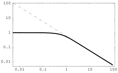
Figure 3: The solid line depicts $P(r)/r_{M}$ (on the vertical axis, where $P\equiv r(1-g_{0}0)$), as a function of $r$ on the horizontal axis. The dashed line presents the function $0.28{r_{*}}/r$; The value of $r_{*}$ is set to 1 on this graph.

As in the AdSS case, the corrections to the Schwarzschild solution that are proportional to $m_{c}$ give rise to the four-dimensional Ricci curvature $R_{m_{c}}$. This is interesting since the curvature is completely due to the modification of gravity. However, unlike the AdSS case, this curvature is not a constant but depends on $r$; moreover it also depends on the strength of the source itself. The plot of the Ricci curvature is given on Fig. 4.

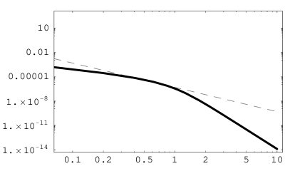
Figure 4: The solid line depicts the magnitude of the four-dimensional Ricci scalar curvature (on the vertical axes) as a function of $r$ on the horizontal axes. The dashed line depicts the dependence of the 4D Kretschmann scalar on $r$. The value of $r_{*}$ is set to 1 on this plot.

The presence of this curvature can easily be understood by looking at the trace of the 4D Einstein equation on the brane

$$R_{4}\,+\,3\,m_{c}\,K\,=\,8\pi\,G_{N}T\,.$$ (66)

$T$ is zero outside a localized source such as a star. However, the trace of the extrinsic curvature $K$ is not zero, therefore, $R_{m_{c}}=-3m_{c}\,K\neq 0$ and $R_{4}$ outside of the source is nonzero and equals to $R_{m_{c}}$.

Similar to the AdSS solution the above properties can be expressed in terms of the invariants

$$R_{K}\,\gg R_{m_{c}}~{}~{}{\rm for}~{}r\ll r_{*}~{}~{}{\rm and}~{}r\gg r_{*}\,;~{}~{}R_{K}\,\sim R_{m_{c}}~{}~{}{\rm for}~{}r\sim r_{*}\,.$$ (67)

Unlike the AdSS solution, however, the curvature $R_{m_{c}}(r)$ decreases very fast after $r\gg r_{*}$. Hence, the induced curvature $R_{m_{c}}(r)$ is subdominant to $R_{K}$ everywhere except in the neighborhood of the point $r\sim r_{*}$ where they both are of the same order $\sim m_{c}^{2}$, see Fig. 4.

Furthermore, unlike the AdSS solution, our solution can be presented in the same coordinate system even for $r\geq r_{c}$. This is because there is no horizon at $r=r_{c}$ and our solution smoothly turns into the 5D Schwarzschild solution

$$ds^{2}|_{y=0}\,=\,\left(1\,-\,{{\tilde{r}}^{2}_{M}\over r^{2}}\right)\,dt^{2}\,-\,{dr^{2}\over\left(1\,-\,{{\tilde{r}}^{2}_{M}\over r^{2}}\right)}\,-\,r^{2}\,d\Omega_{2}^{2}\,.$$ (68)

The key property of this solution is that the gravitational radius is rescaled

$${\tilde{r}}_{M}\,\sim\,r_{M}\,\left({r_{c}\over r_{M}}\right)^{1/3}\,\gg\,r_{M}\,.$$ (69)

This has an explanation. The gravitational radius grows compared to $r_{M}$ because in the 5D regime the gravitational coupling constant grows. However, there is an opposite effect as well. In fact, the gravitational radius reduces compared to what it would have been in a pure 5D theory with no brane. This is because the effective mass of the source $M_{\rm eff}$, defined as ${\tilde{r}}_{M}^{2}\equiv M_{\rm eff}/M_{*}^{3}$, gets screened. Indeed, $M_{\rm eff}$ includes contributions from the curvature $R_{m_{c}}(r)$ that stretches out all the way to $r=r_{c}$. The screened mass of the source is

$$M_{\rm eff}\,\sim\,M\,\left({r_{M}\over r_{c}}\right)^{1/3}\,\ll\,M\,.$$ (70)

Thus, as seen from $r\gg r_{c}$ distances, there is strong screening of the source.

All the above results could be understood as follows. Consider an empty brane and an empty bulk. The Minkowski space is a solution. Let us place a static source on the brane at $r=0$. The Minkowski solution remains globally stable, however, the source, no matter how weak, triggers local instability of the Minkowski space on a brane in the region $r\leq r_{*}$. In this patch the Minkowski space is readjusted to a curved space. The curvature of the latter depends on the strength of the source, it slowly decreases with increasing $r$ but drops fast at $r>r_{*}$. For an observer at large distances it looks as if the source has polarized the medium (brane) around it. This observer measures the screened mass (69) which also includes the contributions of the curvature.

At large enough distances, i.e. $\sqrt{r^{2}+y^{2}}\gg r_{*}$, the solution turns into a 5D spherically-symmetric Schwarzschild solution,

$$ds^{2}|_{\sqrt{r^{2}+y^{2}}\gg r_{*}} \sim \left(1\,-\,{{\tilde{r}}^{2}_{M}\over r^{2}\,+\,y^{2}}\right)\,dt^{2}\,$$ (71)

$$- {dr^{2}\over\left(1\,-\,{{\tilde{r}}^{2}_{M}\over r^{2}\,+\,y^{2}}\right)}\,-\,(r^{2}+y^{2})\,d\Omega_{3}^{2}\,.$$

However, the 5D spherical symmetric is only an approximation and does not hold for $\sqrt{r^{2}+y^{2}}\ll r_{*}$. In the latter regime the properties of the solution on and off the brane are rather different. The pure 5D spherically-symmetric solution (71) is squeezed both on and off the brane but it is more squeezed on the brane than in the bulk. Hence, the only symmetry of the solution that is left is the cylindrical symmetry.

4 Brane-induced gravity in more than five dimensions – softly massive gravity

In the present section we turn to Brane Induced Gravity in more than 5 dimensions. These models share the main property of the 5D model that gravity at short distances is four-dimensional, becoming higher dimensional at larger scales. However, there are a number of crucial distinctions from the 5D case. These are:

• Unlike a 3-brane embedded in 5D space-time, the embedding into six and higher dimensional space-times allows to preserve the 3-brane world-volume to be flat. This suggest that the CCP could be solved in this approach in dimensions six and higher [15, 20].

• Unlike the 5D case, the transverse to the brane Green’s functions in six dimensions and higher are sensitive to the UV physics. A careful treatment of the UV regularization procedure [15, 58, 59, 60] is needed. The best option is to use the UV completion dictated by the String Theory construction [26].

• In most of the interesting cases where simplest UV regularizations were tried so far, the flat space propagator exhibits new poles that correspond to very light $m\sim H_{0}$ tachyons [61] with negative residues [62]. The positions of these poles and their mere existence is UV regularization dependent. At present, it is not clear whether these poles would persist in a consistent UV completed theory, such as in the string theory construction [26]. Work to establish this is in progress [63]. However, even in the regularizations where the new poles exist, they can be eliminated by a special prescription for the poles of the Greens functions [57] at the expense of sacrificing causality at the Hubble scales. This suggest that if these poles are truly present in the theory, then the flat space-time, although globally stable, might not be a locally stable background within a patch of the size $H_{0}^{-1}$. Such a local instability takes place in the 5D model but only at a nonlinear level and at a different scale [46]. This issue in the context of six- and higher-dimensional models awaits further investigation.

• Unlike the 5D case, it turns out that in six and higher dimensions perturbation theory does not break down at low scale [57]. This observation is independent of the UV regularization as well as of the presence/absence of the new poles discussed in the previous item (i.e., the naive perturbation theory does not break down at a low scale even when the new poles are not present, see below).

The first issue on the list above was already discussed in Sect. 2. In what follows we will study in turn the second, third and fourth issues. As was mentioned above, these three items apply to a brane that has no tension (i.e, to a brane the cosmological constant on which is fine-tuned to zero). However, our main goal is to study a brane with an arbitrary tension, and the last three properties listed above should be studied and established for this case. This is only partially fulfilled so far, with certain encouraging results (see below). Further detailed calculations are still needed. Here we derive results for a tensionless brane following Ref. [57].

The equation of motion for the theory described by the action (8) in $D\geq 6$ takes the form

$$\delta^{(N)}(y)\,M_{\rm Pl}^{2}\,G^{(4)}_{\mu\nu}\,\delta^{\mu}_{A}\,\delta^{\nu}_{B}\,+\,M_{*}^{2+N}\,G^{(D)}_{AB}\,=\,-T_{\mu\nu}(x)\,\delta^{\mu}_{A}\,\delta^{\nu}_{B}\,\delta^{(N)}(y)\,.$$ (72)

$G^{(4)}_{\mu\nu}$ and $G^{(D)}_{AB}$ denote the four-dimensional and $D$-dimensional Einstein tensors, respectively. We choose (for simplicity) a source localized on the brane, $T_{\mu\nu}(x)\delta^{(N)}(y)$.

Gravitational dynamics encoded in Eq. (72) can be inferred both from the four-dimensional (4D) as well as $(4+N)$-dimensional standpoints. From the 4D perspective, gravity on the brane is mediated by an infinite number of the Kaluza–Klein (KK) modes that have no mass gap. Under conventional circumstances (i.e., with no brane kinetic term) this would lead to higher-dimensional interactions. However, the large 4D Einstein–Hilbert (EH) term suppresses the wave functions of heavier KK modes, so that in effect they do not participate in the gravitational interactions on the brane at observable distances [64]. Only light KK modes, with masses $m_{KK}\mathrel{\hbox to0.0pt{\lower 3.0pt\hbox{\hskip 0.0pt$\sim$}\hss}\raise 1.0pt\hbox{$<$}}m_{c}$,

$$m_{c}\equiv\frac{M_{*}^{2}}{M_{\rm Pl}}\,,$$ (73)

remain essential, and they collectively act as an effective 4D graviton with a typical mass of the order of $m_{c}$ and a certain smaller width.

Assuming that $M_{*}\sim 10^{-3}$ eV or so, we obtain $m_{c}\sim H_{0}\sim 10^{-42}$ GeV. Therefore, the DGP model with $N\geq 2$ predicts [60] a modification of gravity at short distances $M_{*}^{-1}\sim 0.1$ mm and at large distances $m_{c}^{-1}\sim H_{0}^{-1}\sim 10^{28}\,\,{\rm cm}$, give or take an order of magnitude. Since gravitational interactions, nevertheless, are mediated by an infinite number of states at arbitrarily low energy scale, the effective theory (8) presents, from the 4D standpoint, a nonlocal theory [20]. Moreover, as was suggested in [21], nonlocalities postulated in pure 4D theory can solve the CCP [21], and give rise to new mechanisms for the present-day acceleration of the universe [21]. (It is interesting to note that the nonlocalities in a gravitational theory that are needed to solve the cosmological constant problem could appear from quantum gravity [65] or matter loops [66] in a purely 4D context.)

On the other hand, from the $(4+N)$-dimensional perspective, gravitational interactions are mediated by a single higher-dimensional graviton. This graviton has two kinetic terms given in Eq. (8), and, therefore, can propagate differently on and off the brane. Namely, at short distances, i.e. at $r<m_{c}^{-1}\sim H_{0}^{-1}\sim 10^{28}\,\,{\rm cm}$, the graviton emitted along the brane essentially propagates along the brane and mediates 4D interactions. However, at larger distances, the extra-dimensional effects take over and gravity becomes ($4+N$)-dimensional.

As was first argued in Ref. [15], the results in $N\geq 2$ DGP models are sensitive to ultraviolet (UV) physics, in contradistinction to the $N=1$ model [14]. In other words, one should either consistently smooth out the width of the brane [60], or introduce a manifest UV cutoff in the theory [58, 59, 60], or do both. With a finite thickness, more localized operators appear on the world-volume of the brane, in addition to the world-volume Einstein–Hilbert term already present in Eq. (8) [60]. For instance, one could think of a higher-dimensional Ricci scalar smoothly spread over the world-volume [45].

In general, terms that are square of the extrinsic curvature can also emerge. Some of these terms can survive in the limit when the brane thickness tends to zero (i.e. in the low-energy approximation). For instance, in the zero-thickness limit of the brane the following terms might be important:

$$\delta^{(N)}(y)\,h^{\mu}_{\mu}\,\partial_{\alpha}^{2}\,h^{a}_{a}\,,~{}~{}~{}\delta^{(N)}(y)\,h^{\mu\nu}\,\partial_{\mu}\partial_{\nu}\,h^{a}_{a}\,,~{}~{}~{}\delta^{(N)}(y)\,h^{\mu}_{\mu}\,\partial_{a}\partial_{b}\,h^{ab}\,,$$ (74)

where $h$ denotes small perturbations on flat space. Although the main features of the model, such as interpolation between the 4D power-law behavior of a nonrelativistic potential at short distances and the higher-dimensional behavior at large distances, are not expected to be changed by adding these terms, nevertheless, the tensorial structure of a propagator could in general depend on these terms and selfconsistency of the theory may require some of these terms to be present in the actions in a reparametrization invariant way.

In the low-energy approximation the exact form of these “extra” terms and their coefficients are ambiguous, because of their UV origin. They will be fixed in a fundamental theory from which the DGP model can be derived [26, 63]. In the present paper, in the absence of such a fundamental theory, (but in the anticipation of its advent), we would like to study a particular parametrization of these “extra” terms, for demonstrational purposes. According to our expectations, physics in the selfconsistent theory will have properties very similar to those discussed below. We will show that these properties are rather attractive since they do avoid severe problems of 4D massive gravity.

Consider the action

$$S = {M_{\rm Pl}^{2}}\,\int\,d^{4}x\,\sqrt{g}\,\left(a\,R(g)\,+\,b\,{\mathcal{R}}_{4+N}\right)$$ (75)

$$+ {M_{*}^{2+N}}\,\int\,d^{4}x\,d^{N}y\,\sqrt{{\bar{g}}}\,{\mathcal{R}}_{4+N}({\bar{g}})\,,$$

where, in addition to the 4D EH term, a D-dimensional EH term localized on the brane is present. Here $a$ and $b$ are some numerical coefficients. We will study the properties of the system described by (75) for different values of $a$ and $b$. The action (75) is fully consistent with the philosophy of Ref. [14]: if there is a (1+3)-dimensional brane in D-dimensional space, with some “matter fields” confined to this brane, quantum loops of the confined matter will induce all possible structures consistent with the geometry of the problem, i.e. (1+3)-dimensional wall embedded in D-dimensional space.

The equation of motion in the model (75) takes the form

$$\delta^{(N)}(y)\,M_{\rm Pl}^{2}\,\left(a\,G^{(4)}_{\mu\nu}\,+\,b\,G^{(D)}_{\mu\nu}\right)\delta^{\mu}_{A}\,\delta^{\nu}_{B}$$

$$+\,M_{*}^{2+N}\,G^{(D)}_{AB}\,=\,-T_{\mu\nu}(x)\,\delta^{\mu}_{A}\,\delta^{\nu}_{B}\,\delta^{(N)}(y)\,.$$ (76)

In deriving the above equation we first introduced a finite brane width $\Delta$, and then took the $\Delta\to 0$ limit in such a way that no surface terms appear. In general, the results depend on the regularization procedure for the brane width. In the present work we adopt a simple prescription in which derivatives with respect to the transverse coordinates calculated on the brane vanish in the $\Delta\to 0$ limit (a unique prescription could only be specified by a fundamental theory.). As previously, $G^{(4)}$ and $G^{(D)}$ denote the four-dimensional and $D$-dimensional Einstein tensors, respectively, while $a$ and $b$ are certain constants. In order to be able to describe 4D gravity at short distances with the right value of Newton’s coupling we set

$$a\,+\,b\,=\,1\,.$$ (77)

Note, that the first two terms in parenthesis on the left-hand side of Eq. (76) can be identically rewritten as

$$(a+b)\,G^{(4)}_{\mu\nu}\,+\,b\left(-\partial_{\mu}\partial_{a}\,h^{a}_{\nu}\,-\,\partial_{\nu}\partial_{a}\,h^{a}_{\mu}\,-\,\partial_{a}^{2}h_{\mu\nu}\,+\,\eta_{\mu\nu}\partial_{a}^{2}h^{C}_{C}\right.$$

$$+\left.\partial_{\mu}\partial_{\nu}h^{a}_{a}\,-\,\eta_{\mu\nu}\partial_{\alpha}^{2}\,h^{a}_{a}\,+\,2\eta_{\mu\nu}\partial_{a}\partial_{\alpha}h^{a\alpha}\,+\,\eta_{\mu\nu}\partial_{a}\partial_{b}h^{ab}\right).$$ (78)

The above equation of motion (76) – which should be viewed as a regularized version of the DGP model – could be obtained from the action (8) as well, provided the latter is amended by certain extrinsic curvature terms. Below we will study this version of the regularized DGP model for various values of the parameters $a$ and $b$.

4.1 Perturbation theory of flat space

We start our discussion with a simple model of a scalar field $\Phi$ in $(4+N)$-dimensional space-time. For convenience we separate the dependence of the scalar field $\Phi$ on four-dimensional and higher-dimensional coordinates, $\Phi(x_{\mu},y_{a})\equiv\Phi(x,y)$. The two kinetic term action – the scalar counterpart of Eq. (8) – is

$$S = {M_{\rm Pl}^{2}}\,\int d^{4}x\,\partial_{\mu}\Phi(x,0)\,\partial^{\mu}\Phi(x,0)$$ (79)

$$+ {M_{*}^{2+N}}\,\int d^{4}x\,d^{N}y\,\partial_{A}\Phi(x,y)\,\partial^{A}\Phi(x,y)\,.$$

It is important to understand that in the scalar case the analog of the new term included in Eq. (76) but absent in (72) reduces, identically, to the already existing localized term. This is a consequence of our choice of the regularization of the brane width $\Delta$ and the boundary conditions according to which transverse derivatives vanish on the brane in the $\Delta\to 0$ limit.

To study interactions mediated by the scalar field we assume that $\Phi$ couples to a source $J$ localized in the 4D subspace in a conventional way, $\int d^{4}x2\Phi(x,0)\,J(x)$. Then the equation of motion takes the form

$$\delta^{(N)}(y)\,M_{\rm Pl}^{2}\,\partial^{2}_{\mu}\,\Phi(x,0)\,+\,M_{*}^{2+N}\,\partial^{2}_{A}\,\Phi(x,y)\,=\,J(x)\,\delta^{(N)}(y)\,.$$ (80)

The very same equation applies to the scalar field Green’s function.

To solve this equation it is convenient to Fourier-transform it with respect to “our” four space-time coordinates $x_{\mu}\to p_{\mu}$, keeping the extra $y$ coordinates intact. Marking the Fourier-transformed quantities by the tilde,

$$\Phi(x,y)\,\to\,{\tilde{\Phi}}(p,y)\,,$$ (81)

we then get from Eq. (80)

$$\delta^{(N)}(y)\,M_{\rm Pl}^{2}(-p^{2})\,{\tilde{\Phi}}(p,0)$$

$$+\,M_{*}^{2+N}\,(-p^{2}-\Delta_{y}){\tilde{\Phi}}(p,y)\,=\,{\tilde{J}}(p)\,\delta^{(N)}(y)\,,$$ (82)

where $p^{2}\equiv p_{0}^{2}-p_{1}^{2}-p_{2}^{2}-p_{3}^{2}$, and the notation

$$\Delta_{y}\,\equiv\,\sum_{a=1}^{N}{\partial^{2}\over\partial y^{2}_{a}}$$ (83)

is used.

We will look for the solution of Eq. (82) in the following form:

$${\tilde{\Phi}}(p,y)\,\equiv\,D(p,y)\,\chi(p)\,,$$ (84)

where the function $D$ is defined as a solution of the equation

$$(-p^{2}-\Delta_{y}-i{\bar{\epsilon}})\,D(p,y)\,=\,\delta^{(N)}(y)\,.$$ (85)

Note that the function $D$ is uniquely determined only after the $i{\bar{\epsilon}}$ prescription specified above is implemented. We also introduce a convenient abbreviation

$$D_{0}(p)\,\equiv\,D(p,y=0)\,.$$ (86)

Now, it is quite obvious that a formal solution of Eq. (82) can be written in terms of the function $D$ as follows:

$${\tilde{\Phi}}(p,y)\,=\,-\,{{\tilde{J}}(p)\over M_{\rm Pl}^{2}}\,\,\,{D(p,y)\over p^{2}\,D_{0}(p)\,-\,M_{*}^{2+N}/M_{\rm Pl}^{2}}\,+c\,{\tilde{\Phi}}_{\rm hom}(p,y)\,,$$ (87)

where ${\tilde{\Phi}}_{\rm hom}(p,y)$ is a general solution of the corresponding homogeneous equation (i.e., Eq. (82) with the vanishing right-hand side), and $c$ is an arbitrary constant. Equation (87) presents, in fact, the Green’s function too, up to the factor $\tilde{J}(p)/M_{\rm Pl}^{2}$, which must be amputated. In particular, for the Green’s function on the brane we have

$$G(p,0)=\frac{M_{\rm Pl}^{2}}{\tilde{J}(p)}\,{\tilde{\Phi}}(p,y=0)\,,\quad G_{\rm hom}(p,0)=\frac{M_{\rm Pl}^{2}}{\tilde{J}(p)}\,{\tilde{\Phi}}_{\rm hom}(p,y=0)\,,$$ (88)

while for arbitrary values of $y$

$$G(p,y)\,=\,-\,{D(p,y)\over p^{2}\,D_{0}(p)-u^{N}}\,+\,c\,G_{\rm hom}(p,y)\,,$$ (89)

where

$$u^{N}\equiv\,\frac{M_{*}^{2+N}}{M_{\rm Pl}^{2}}=m_{c}^{2}\,M_{*}^{N-2}\,.$$ (90)

The presence/absence of the homogeneous part is regulated by the $i\epsilon$ prescription. Note that if the first term on the right-hand side of Eq. (89) has poles on the real axis of $p^{2}$, then the homogeneous equation has a solution

$$G_{\rm hom}(p,y)\,=\,D(p,y)\,\delta\left(p^{2}D_{0}(p)-u^{N}\right)\,.$$ (91)

This fact will play an essential role for gravity.

In what follows we will examine the poles of the Green’s function $G(p,y)$. The positions of these poles depend on the functions $G_{\rm hom}(p,y)$, and $D_{0}$ as defined in Eqs. (85) and (86). The choice of a particular rule of treatment of the poles corresponds to the choice of appropriate boundary conditions in the coordinate space. Note that the latter are dictated by physical constraints on the Green’s function $G$ rather than on the auxiliary function $D$.

To get to the main point, we will try the simplest strategy of specifying the poles and check, a posteriori, whether this strategy is selfconsistent. Let us put

$$c=0$$

and define $D$ in the Euclidean momentum space. Since in the Euclidean space the expression for $D$ is well-defined and has no singularities,

$$D(p_{E},q)=\frac{1}{p_{E}^{2}+q^{2}}\,,\qquad D(p_{E},q)\equiv\int d^{N}y\,e^{iqy}\,D(p_{E},y)\,,$$ (92)

$$q^{2}=\sum_{a}(q^{a})^{2}\,,$$

one can perform analytic continuation from the Euclidean space to Minkowski. This is not the end of the story, however. It is the Green’s function $G$ that we are interested in, not the auxiliary function $D$. As will be explained below, the above procedure is consistent, for the following reason. The function $G$ obtained in this way has a cut extending from zero to infinity. In addition, we find two complex conjugate poles on the second unphysical Riemann sheet of the complex $p^{2}$ plane. Moreover, there are additional poles on subsequent unphysical sheets.

4.2 Six dimensions

It is instructive to demonstrate how things work by considering separately the six-dimensional case. In six dimensions sensitivity to the UV cutoff is only logarithmic, and it is conceivable that the results obtained in the cut-off theory could be consistently matched to those of a more fundamental UV-completed theory-to-come.

It is not difficult to calculate

$$D_{0}(s)\,=\frac{1}{4\pi}\,\ln\left({\Lambda^{2}\over-s}\,+1\,\right)\,,\qquad s\equiv p^{2}\,,$$ (93)

where $\Lambda^{2}$ is an ultra-violet cut-off. With this expression for $D_{0}$ the function $G(p^{2},0)$ develops a cut on the positive semiaxes of $s$ due to the logarithmic behavior of $D_{0}(s)$. This fact has a physical interpretation. Since the extra dimensions are noncompact in the model under consideration, the spectrum of the theory, as seen from the 4D standpoint, consists of an infinite gapless tower of the KK modes. This generates a cut in the Green’s function for $s$ ranging from zero to $+\infty$.

In addition, there might exist isolated singular points in $G(p^{2},0)$. These singularities (for $s\ll\Lambda^{2}$) are determined by the equation

$$G^{-1}(s,0)\equiv s-m_{c}^{2}\,\left[\frac{1}{4\pi}\ln\left(\frac{\Lambda^{2}}{-s}\right)\right]^{-1}=\,0\,,$$ (94)

where $m_{c}^{2}$ is defined in Eq. (73). Let us introduce the notation

$$s\,\equiv\,s_{0}\,{\rm exp}(i\gamma)\,,$$ (95)

where $s_{0}$ is a real positive number. Then, Eq. (94) has two solutions of the form

$$s_{0}\approx 4\pi\,m_{c}^{2}\left[\ln\frac{\Lambda^{2}}{m_{c}^{2}}\right]^{-1}\,,$$ (96)

and

$$\gamma_{1}\,\simeq\,-\,{\pi\over{\rm log}(\Lambda^{2}/m_{c}^{2})}\,,~{}~{}~{}\gamma_{2}\,\simeq\,2\pi\,+\,{\pi\over{\rm log}(\Lambda^{2}/m_{c}^{2})}\,.$$ (97)

We conclude that there are two complex-conjugate poles on the nearby unphysical Riemann sheets. These poles cannot be identified with any physical states of the theory. They are, in fact, manifestations of a massive resonance state. All other complex poles appear on subsequent nonphysical Riemann sheets.

4.3 More than six dimensions

Physics at $D>6$ is similar to that of the six-dimensional world which was described in Sect. 4.2. There are minor technical differences between odd- and even-dimensional spaces, however, as we will discuss momentarily.

In seven dimensions we find

$$D_{0}(s)\,=\,{1\over 2\,\pi^{2}}\,\left\{\Lambda\,-\,\sqrt{-s}\,{\rm arctan}\left({\Lambda\over\sqrt{-s}}\right)\right\}\,.$$ (98)

As in the 6D case, there is a branch cut. The cut in this case is due to the dependence of the Green’s function on $\sqrt{s}$. No other singularities appear on the physical Riemann sheet. All poles are on unphysical Riemann sheets, as previously.

In the eight-dimensional space the expression for $D_{0}$ reads

$$D_{0}(s)\,=\,{1\over 16\,\pi^{2}}\,\left\{\Lambda^{2}\,+\,s\,\left({\rm ln}\,{\Lambda^{2}\over-s}\,+\,1\,\right)\right\}\,.$$ (99)

Again, we find a cut due to the logarithm, similar to that of the 6D case. All isolated singularities appear on unphysical Riemann sheets.

The nine-dimensional formula runs parallel to that in seven dimensions,

$$D_{0}(s)\,=\,{1\over 12\,\pi^{3}}\,\left\{{\Lambda^{3}\over 3}\,+\,s\left(\Lambda\,-\,\sqrt{-s}\,{\rm arctan}\,{\Lambda\over\sqrt{-s}}\right)\right\}\,.$$ (100)

Finally, in ten dimensions

$$D_{0}(s)\,=\,{1\over 128\,\pi^{3}}\,\left\{{\Lambda^{4}\over 2}\,+\,s\left[\,\Lambda^{2}\,+\,s\,\left({\rm ln}\,{\Lambda^{2}\over-s}\,+\,1\,\right)\right]\right\}\,.$$ (101)

The pole structure of $G$ is identical to that of the eight-dimensional case. Since the pattern is now well established and clear-cut, there seems to be no need in dwelling on higher dimensions.

Before turning to gravitons we would like to make comments concerning the UV cutoff $\Lambda$. The crossover distance $r_{c}\sim m_{c}^{-1}$ depends on this scale: in 6D the dependence is logarithmic, while in $D>6$ this dependence presents a power law [15, 26]. Hence, the crossover scale in the $N\geq 2$ DGP models, unlike that in the $N=1$ model, is sensitive to particular details of the UV completion of the theory. Since in the present work we adopt an affective low-energy field-theory strategy, we are bound to follow the least favorable scenario in which the cutoff and the bulk gravity scale coincide with each other and both are equal to $M_{*}\sim 10^{-3}$ eV. If a particular UV completion were available, it could well happen that the UV cutoff and bulk gravity scale were different from the above estimate. In fact, in the string-theory-based construction of Ref.  [26] the UV completion is such that the cutoff and bulk gravity scale are in the ballpark of TeV.

In conclusion of this section it is worth noting that the Green’s function $D_{0}$ in the $N\geq 3$ case contains terms responsible for branch cuts. These terms are suppressed by powers of $s/\Lambda$, and, naively, could have been neglected. It is true, though, that the explicit form of these terms is UV-sensitive and cannot be established without the knowledge of UV physics. One should be aware of these terms since they reflect underlying physics – the presence of the infinite tower of the KK states. Fortunately, none of the results of the present work depend on these terms.

4.4 The graviton propagator

Now it is time to turn to gravitons with their specific tensorial structure. We will consider and analyze the equation of motion of the DGP-type model presented in Eq. (76), which we reproduce here again for convenience

$$\delta^{(N)}(y)\,M_{\rm Pl}^{2}\,\left(a\,G^{(4)}_{\mu\nu}+b\,G^{(D)}_{\mu\nu}\right)\delta^{\mu}_{A}\,\delta^{\nu}_{B}$$

$$+\,M_{*}^{2+N}\,G^{(D)}_{AB}\,=\,-T_{\mu\nu}(x)\,\delta^{\mu}_{A}\,\delta^{\nu}_{B}\,\delta^{(N)}(y)\,.$$ (102)

Here $G^{(4)}$ and $G^{(D)}$ denote the four-dimensional and $D$-dimensional Einstein tensors, respectively, while $a$ and $b$ are certain constants satisfying the constraint

$$a+b=1\,.$$

For simplicity we choose a source term localized on the brane, namely, $T_{\mu\nu}(x)\delta^{(N)}(y)$. At the effective-theory level the ratio $a/b\equiv a/(1-a)$ is a free parameter. The only guidelines we have for its determination are (i) phenomenological viability; (ii) intrinsic selfconsistency of the effective theory which, by assumption, emerges as a low-energy limit of a selfconsistent UV-completed underlying “prototheory.” Specifying the prototheory would allow one to fix the ratio $a/(1-a)$ in terms of fundamental parameters.

Our task is to study the gravitational field produced by the source $T_{\mu\nu}(x)\delta^{(N)}(y)$. To this end we linearize Eq. (102). If $g_{AB}\equiv\eta_{AB}+2h_{AB}$, in the linearized in $h$ approximation we find

$$G^{(D)}_{AB} = \partial_{D}^{2}\,h_{AB}\,-\,\partial_{A}\,\partial_{C}\,h^{C}_{B}\,-\,\partial_{B}\,\partial_{C}\,h^{C}_{A}$$ (103)

$$+ \partial_{A}\,\partial_{B}\,h^{C}_{C}\,-\,\eta_{AB}\,\partial_{D}^{2}\,h^{C}_{C}\,+\,\eta_{AB}\,\partial_{C}\,\partial_{D}\,h^{CD}\,,$$

where $\partial_{D}^{2}\equiv\partial_{D}\partial^{D}$. On the other hand, the four-dimensional Einstein tensor in the linearized approximation is

$$G^{(4)}_{\mu\nu} = \partial_{\beta}^{2}\,h_{\mu\nu}\,-\,\partial_{\mu}\,\partial_{\alpha}\,h^{\alpha}_{\nu}\,-\,\partial_{\nu}\,\partial_{\alpha}\,h^{\alpha}_{\mu}\,+\,\partial_{\mu}\,\partial_{\nu}\,h^{\alpha}_{\alpha}\,$$ (104)

$$- \eta_{\mu\nu}\,\partial_{\beta}^{2}\,h^{\alpha}_{\alpha}\,+\,\eta_{\mu\nu}\,\partial_{\alpha}\,\partial_{\beta}\,h^{\alpha\beta}\,.$$

In what follows we will work in the harmonic gauge,

$$\partial^{A}\,h_{AB}\,=\,{1\over 2}\,\partial_{B}\,h^{C}_{C}\,.$$ (105)

The advantage of this gauge is that in this gauge the expression for $G^{(D)}_{AB}$ significantly simplifies,

$$G^{(D)}_{AB}\,=\,\partial_{D}^{2}\,h_{AB}\,-\,{1\over 2}\,\eta_{AB}\,\partial_{D}^{2}\,h^{C}_{C}\,.$$ (106)

Additional conditions which are invoked to solve the $\{ab\}$ and $\{a\mu\}$ components of the equations of motion are

$$h_{a\mu}=0,~{}~{}~{}~{}~{}h_{ab}\,=\,{1\over 2}\,\eta_{ab}\,h^{C}_{C}\,.$$ (107)

Using the last equation it is not difficult to obtain the relation

$$N\,h^{\mu}_{\mu}\,=\,(2-N)\,h^{a}_{a}\,.$$ (108)

This relation obviously suggests that we should consider separately two cases:

(i) $N=2$;

(ii) $N>2$.
We will see, however, that the results in the $N=2$ and $N>2$ cases are somewhat similar.

4.5 Brane-induced gravity in six dimensions ($N=2)$

In two extra dimensions Eq. (108) implies

$$h^{\mu}_{\mu}\,=\,0\,.$$ (109)

Therefore, the trace of the $D$-dimensional graviton coincides with the trace of the extra-dimensional part,

$$h^{A}_{A}\,=\,h^{a}_{a}\,.$$ (110)

As a result, the four-dimensional components of the harmonic gauge condition (105) reduce to

$$\partial^{\mu}\,h_{\mu\nu}\,=\,{1\over 2}\,\partial_{\nu}\,h^{a}_{a}\,.$$ (111)

Let us now have a closer look at the $\{\mu\nu\}$ part of Eq. (76). Taking the trace of this equation and using Eqs. (106), (104), (109) and (111) we arrive at

$$(3b\,-\,1)\,\delta^{(N)}(y)\,M_{\rm Pl}^{2}\,\partial^{2}_{\mu}\,h^{a}_{a}\,+\,2\,M_{*}^{2+N}\,\partial^{2}_{A}\,h^{a}_{a}\,=\,T^{\mu}_{\mu}\,\delta^{(N)}(y)\,.$$ (112)

The obtained equation is very similar to the scalar-field equation (80). Therefore, we will follow the same route as in the scalar-field case, until we come to a subtle point, a would-be obstacle, which was nonexistent in the scalar-field case.

Let us Fourier-transform Eq. (112),

$$(3b\,-\,1)\,\delta^{(N)}(y)\,M_{\rm Pl}^{2}(-p^{2})\,{\tilde{h}}^{a}_{a}(p,y)$$

$$+2M_{*}^{2+N}\,(-p^{2}-\Delta_{y})\,{\tilde{h}}^{a}_{a}(p,y)={\tilde{T}}(p)\,\delta^{(N)}(y)\,.$$ (113)

The general solution of the above equation is

$${\tilde{h}}^{a}_{a}(p,y)={{\tilde{T}}(p)\over M_{\rm Pl}^{2}}\,{\cal G}(p,y)\,,$$ (114)

$${\cal G}={D(p,y)\over 2m_{c}^{2}\,-\,(3b\,-\,1)p^{2}\,D_{0}(p)\,}\,+\,c\,{\cal G}_{\rm hom}\,,$$ (115)

where the solution of the homogeneous equation takes the form

$${\cal G}_{\rm hom}\,=\,D(p,y)\,\delta\left(2m_{c}^{2}\,-\,(3b\,-\,1)p^{2}D_{0}(p)\right)\,.$$ (116)

To begin with, let us consider the case $3b>1$. Then the first term on the right-hand side of Eq. (115) has poles for complex values of $p^{2}$. For instance, in the 6D case this pole is determined by the equation

$$s={2m_{c}^{2}\over(3b-1)D_{0}(s)}={4\pi\,{2m_{c}^{2}}\over(3b-1)}\,\left[\ln\frac{\Lambda^{2}}{-s}\right]^{-1}\,.$$ (117)

This equation has at least two solutions of the form

$$s_{*}\approx{4\pi\,2m_{c}^{2}\over 3b-1}\left[\ln\frac{\Lambda^{2}}{m_{c}^{2}}\right]^{-1}\,,$$ (118)

and

$$\gamma_{1}\,\simeq\,-\,{\pi\over{\rm log}(\Lambda^{2}/m_{c}^{2})}\,,~{}~{}~{}\gamma_{2}\,\simeq\,2\pi\,+\,{\pi\over{\rm log}(\Lambda^{2}/m_{c}^{2})}\,.$$ (119)

The quantity ${\tilde{h}}^{a}_{a}(p,y)$ is not a gauge invariant variable. Therefore, the presence of certain poles in the expression for ${\tilde{h}}^{a}_{a}(p,y)$ depends on a gauge. However, explicit calculations (see below) show that the poles found above also enter the gauge invariant physical amplitude. Therefore, we need to take these poles seriously and analyze their physical consequences.

4.6 $b>1/3$

If $b>1/3$ there are no poles on the physical Riemann sheet. Instead, poles appear on the nearest unphysical Riemann sheets. These poles cannot be identified with any physical states of the theory. They represent a signature of massive resonance states. All other complex poles appear on subsequent nonphysical Riemann sheets.

Using a contour integral one can easily write down the spectral representation for the Green’s function ${\mathcal{G}}$

$${{\cal G}}(p,y=0)\,=\,{1\over\pi}\,\int_{0}^{\infty}\,{\rho(t)\,dt\over\,t\,-\,p^{2}\,-\,i\,{\bar{\epsilon}}}\,,$$ (120)

where the spectral function is defined as

$$\rho(t)\,=\,{2\,m_{c}^{2}\,{\rm Im}\,D_{0}(t)\over\left[(3b-1)t\,{\rm Re}\,D_{0}\,-\,2m_{c}^{2}\right]^{2}\,+\left[(3b-1)t\,{\rm Im}\,D_{0})\right]^{2}}\,,$$ (121)

and

$${\rm Im}D_{0}\,=\,\pi\,\int\,{d^{N}q\over(2\pi)^{N}}\,\delta(t-q^{2})\,=\,{\pi^{N+2\over 2}\over(2\pi)^{N}\Gamma(N/2)}\,t^{N-2\over 2}\,.$$ (122)

We see that $\rho(t)$ satisfies the positivity requirement. Equation (120) guarantees that the Green’s function ${\cal G}$ is causal.

The next step is applying the expression for ${\cal G}$ to calculate ${\tilde{h}}_{\mu\nu}$. In fact, it is more convenient to calculate the tree-level amplitude

$$A(p,y)\,\equiv\,{\tilde{h}}_{\mu\nu}(p,y)\,{\tilde{T}}^{\prime\,\mu\nu}(p)\,,$$ (123)

where ${\tilde{T}}^{\prime\,\mu\nu}(p)$ is a conserved energy momentum tensor,

$$p_{\mu}\,{\tilde{T}}^{\prime\,\mu\nu}\,=\,p_{\nu}\,{\tilde{T}}^{\prime\,\mu\nu}\,=\,0\,.$$

Using Eqs. (102), (114) and (134) we obtain a lengthy expression for the amplitude $A(p,y)$,

$$A(p,y) = {1\over M_{\rm Pl}^{2}}\,{D(p,y)\over p^{2}\,D_{0}(p)\,-\,m_{c}^{2}}\,\left\{{\tilde{T}}_{\mu\nu}{\tilde{T}}^{\prime\,\mu\nu}\right.$$ (124)

$$- \left.{{\tilde{T}}\,{\tilde{T}}^{\prime}\over 2}\,\left[{(2b-1)p^{2}D_{0}-m_{c}^{2}\over(3b-1)p^{2}D_{0}-2m_{c}^{2}}\right]\right\}.$$

Let us study the above expression in some detail. The first question to ask is about poles. It is quite clear that the $p^{2}$-poles of $A$ are of two types; their position is determined by:

$$p^{2}\,D_{0}(p)\,=\,m_{c}^{2}$$

or

$$(3b-1)p^{2}\,D_{0}(p)\,=\,2m_{c}^{2}\,.$$

As was explained previously, all these poles appear on the second Riemann sheet, with the additional images on other unphysical sheets. None of these poles can be identified with asymptotic physical states. As was elucidated above, the occurrence of the poles on the second and subsequent Riemann sheets corresponds to the massive-resonance nature of the effective 4D graviton. Our previous analysis can be repeated practically verbatim, with minor modifications, proving analyticity and causality of the amplitude $A$.

Next, we observe that at large momenta, i.e., when $p^{2}\,D_{0}(p)\gg m_{c}^{2}$, the scalar part of the propagator has 4D behavior; the tensorial structure is not four-dimensional, however. The terms in the braces in Eq. (124), namely,

$$\left\{{\tilde{T}}_{\mu\nu}{\tilde{T}}^{\prime\,\mu\nu}\,-\,{2b-1\over 2(3b-1)}\,{\tilde{T}}\,{\tilde{T}}^{\prime}\,\right\}\,,$$ (125)

correspond to the exchange of massive gravitons and scalar degrees of freedom. This would give rise to additional contributions in the light bending, and is excluded phenomenologically, unless the contribution due to extra polarizations is canceled by some other interactions (such as, e.g., an additional repulsive vector exchange). Note also that when $b\gg a$, i.e., $b\to 1$, one obtains the tensorial structure of 6D gravity, as expected from (75).

On the other hand, at large distances, i.e., at $p^{2}\,D_{0}(p)\ll m_{c}^{2}$, we get the following tensorial structure of the amplitude (124):

$$\left\{{\tilde{T}}_{\mu\nu}{\tilde{T}}^{\prime\,\mu\nu}\,-\,{1\over 4}\,{\tilde{T}}\,{\tilde{T}}^{\prime}\,\right\}\,.$$ (126)

This exactly corresponds to the exchange of a six-dimensional graviton, as was expected.

4.7 $b<1/3$

This case is conceptually different from that of Sect. 4.6. As we will see momentarily, if $b<1/3$ there are no problems in (i) maintaining 4D unitarity; and (ii) getting the appropriate 4D tensorial structure of gravity at subhorizon distances. This is achieved at a price of abandoning 4D analyticity, in its standard form, which could presumably lead to the loss of causality at distances of the order of $m_{c}^{-1}\sim 10^{28}$ cm. The absence of causality at distances $\mathrel{\hbox to0.0pt{\lower 4.0pt\hbox{\hskip 1.0pt$\sim$}\hss}\raise 1.0pt\hbox{$>$}}10^{28}$ cm, was argued recently [21] to be an essential ingredient for solving the cosmological constant problem.

Although all derivations and conclusions are quite similar for any ratio $a/b$ as long as $2b<a$, we will stick to the technically simplest example $b=0$, $a=1$. In the situation at hand, the homogeneous part (116) need not be trivial, i.e $c$ need not vanish. The value of the constant $c$ is determined once the rules for the pole at $p^{2}D_{0}(p)+2m_{c}^{2}=0$ are specified. Putting $c=0$ leads to nonunitary Green’s function. Therefore, we abandon the condition $c=0$ in an attempt to make a more consistent choice that would guarantee 4D unitarity. We stress that we are after unitarity here, not unitarity plus causality.

To begin with we pass to the Euclidean space in $p^{2}$ (i.e. $p^{2}\to p_{E}^{2}$) and introduce the following notation:

$$P^{(E)}(p_{E}^{2})\,\equiv\,{1\over 2\,m^{2}_{c}\,-\,p_{E}^{2}\,D_{0}(p_{E})-\,i{\epsilon}}\,.$$ (127)

The function $P^{(E)}$ is a Euclidean-space solution of Eq. (113), with the particular choice $c=i\pi$. (The choice $c=-i\pi$ would lead to Eq. (127) with the replacement ${\epsilon}\to-{\epsilon}$).

As the next step we will analyze the complex plane of $p_{E}^{2}$. Since the function $D_{0}(p_{E})$ is real, the function $P^{(E)}(p_{E}^{2})$ must (and does) have an isolated singularity in the $p_{E}^{2}$ plane which is similar to a conventional massive pole, except that it lies in the Euclidean domain. This singularity occurs at the point $p_{E}^{2}=p_{*}^{2}$ is defined by the condition

$$p_{*}^{2}D_{0}(p_{*})\,=\,2\,m_{c}^{2}\,,~{}~{}~{}~{}~{}p_{*}^{2}\,\,\,\mbox{real and positive}.$$ (128)

This is the only isolated singularity in Eq. (127); it is located in the complex $p_{E}^{2}$ plane on the real positive semiaxis. In addition to this pole singularity, the function (127) has a branch cut stretching from zero to $-\infty$ due to the imaginary part of $D_{0}(p_{E}^{2})$ appearing at negative values of $p_{E}^{2}$. As before, this branch cut is the reflection of an infinite gapless tower of the KK states. As a result, the following spectral representation obviously emerges for $P^{(E)}(p_{E}^{2})$:

$$P^{(E)}(p_{E}^{2}+i{\epsilon})\,=\,{1\over\pi}\,\int_{0}^{-\infty}\,{{\rm Im}P^{(E)}(u)\,du\over u\,-\,p_{E}^{2}\,}\,+\,{R\over p_{*}^{2}\,-\,p_{E}^{2}\,-\,i{\epsilon}}\,,$$ (129)

with the Euclidean pole term being “unconventional.” The residue of the pole $R$ is given (for any $N$) by

$$R^{-1}\,=\,\int\,{d^{N}q\over(2\pi)^{N}}\,{q^{2}\over(q^{2}\,+\,p_{*}^{2})^{2}}\,.$$ (130)

Note that in the first term on the right-hand side of Eq. (129) the integration runs from zero to minus infinity; thus, the integrand never hits the would-be pole at $u=p_{E}^{2}>0$. Therefore, the $i{\epsilon}$ prescription is in fact used only to specify the isolated pole at $p_{E}^{2}=p_{*}^{2}$.

We proceed further and define a symmetric function

$$\Pi^{(E)}(p_{E}^{2})\,\equiv\,{1\over 2}\left\{P^{(E)}(p_{E}^{2}-i{\epsilon})\,+\,P^{(E)}(p_{E}^{2}+i{\epsilon})\right\}\,.$$ (131)

It is just this symmetric function on which we will focus in the remainder of the section. Let us return to the Minkowski space. This is done by substituting

$$p_{E}^{2}\to{\rm exp}(-i\pi)p^{2}\,,\qquad u\to{\rm exp}(-i\pi)t$$

in Eq. (129). Furthermore, observing that ${\rm Im}\,P={\rm Im}\,\Pi$, we obtain the following representation for the Minkowskian $\Pi$:

$$\Pi(p)\,=\,{1\over\pi}\,\int_{0}^{\infty}\,{{\rm Im}\Pi(t)\,dt\over t\,-\,p^{2}\,-\,i\,{\bar{\epsilon}}}\,+\,\Pi_{0}(p)\,,$$ (132)

where

$$\Pi_{0}(p)\,\equiv\,{1\over 2}\left({R\over p_{*}^{2}\,+p^{2}\,-\,i{\epsilon}}\,+\,{R\over p_{*}^{2}\,+p^{2}\,+\,i{\epsilon}}\right)\,.$$ (133)

It is necessary to emphasize that $\epsilon$ and $\bar{\epsilon}$ are two distinct regularizing parameters, $\epsilon\neq\bar{\epsilon}$. The parameter $\epsilon$ is used to regularize the pole at $p^{2}=-p_{*}^{2}$, while $\bar{\epsilon}$ sets the rules for the branch cut. The most important property of $\Pi$ is that the pole at $p^{2}=-p_{*}^{2}$ has no imaginary part, by construction. Hence, there is no physical particle that corresponds to this pole. In the conventional local field theory the only possible additions with no imaginary part are polynomials. Here we encounter a new structure which will be discussed in more detail at the end of this section.

Our goal is to show that a 4D-unitarity-compliant spectral representation holds for the Green’s function on the brane, at least in the domain where the laws of 4D physics are applicable. To this end we turn to the function ${\cal G}(p,y)$, defined as

$${\cal G}\,=\,{D(p,y)}\,\Pi(p^{2})\,.$$ (134)

with the purpose of studying its properties. It is convenient to pass to the momentum space with respect to extra coordinates too. Then, the propagator (134) takes the form

$${\tilde{\cal G}}(p,q)\,=\,{\Pi(p^{2})\over q^{2}\,-\,p^{2}\,-i\,{\bar{\epsilon}}}\,.$$ (135)

With these definitions in hand, we can write down the 4D dispersion relation. We start from the Källen–Lehman representation for the propagator (135). As we will check below, this representation takes the form

$${\tilde{\cal G}}(p,q)\,=\,{1\over\pi}\,\int_{0}^{\infty}\,{{\rm Im}{\tilde{\cal G}}(t,q)\,dt\over t\,-\,p^{2}\,-\,i\,{\bar{\epsilon}}}\,+\,{\Pi_{0}(p^{2})\,-\,\Pi_{0}(q^{2})\over q^{2}\,-\,p^{2}\,-\,i\,{\bar{\epsilon}}}\,.$$ (136)

The imaginary part of ${\tilde{\cal G}}$ is defined as follows

$${\rm Im}{\tilde{\cal G}}(t,q)\,=\,\pi\,\delta(q^{2}\,-\,t)\,{\rm Re}\Pi(t)\,+\,{\rm Im}\Pi(t)\,{\mathcal{P}}{1\over q^{2}\,-\,t}\,,$$ (137)

where ${\mathcal{P}}$ stands for the principle value of a singular function,

$${\mathcal{P}}\,{1\over q^{2}\,-\,t}\,=\,{1\over 2}\left({1\over q^{2}\,-\,t\,+\,i\delta}\,+\,{1\over q^{2}\,-\,t\,-\,i\delta}\right).$$ (138)

The fact that Eq. (136) holds can be checked by substituting (138) and (137) into (136) and exploiting the relation

$${1\over\pi}\,\int_{0}^{\infty}\,{{\rm Im}{\Pi}(t)\over t\,-\,p^{2}\,-\,i\,{\bar{\epsilon}}}\,{\mathcal{P}}{1\over q^{2}\,-\,t}\,dt$$

$$=\,-{{\rm Re}\Pi(q^{2})\,-\,\Pi_{0}(q^{2})\,+\,\Pi_{0}(p^{2})\,-\,\Pi(p^{2})\over q^{2}-p^{2}-i\,{\bar{\epsilon}}}\,.$$ (139)

This turns Eq. (136) into identity.

Finally we approach the main point of this section – the dispersion relation for ${\cal G}(p,y=0)$, the Green’s function on the brane. As such, it must have a spectral representation with the positive spectral density, as we have already seen from the KK-based analysis. The positivity is in one-to-one correspondence with the 4D unitarity.

The dispersion relation can be obtained by integrating (136) with respect to $q$,

$${{\cal G}}(p,y=0)\,=\,{1\over\pi}\,\int_{0}^{\infty}\,{\rho(t)\,dt\over\,t\,-\,p^{2}\,-\,i\,{\bar{\epsilon}}}\,+\,\Pi_{0}(p^{2})\,{\rm Re}D_{0}(-p_{*}^{2})\,.$$ (140)

According to Eq. (136), the spectral density $\rho$ is defined as

$$\rho(t)\,=\,\int\,{d^{N}q\over(2\pi)^{N}}\,{\rm Im}\,{\tilde{\cal G}}(t,q)\,.$$ (141)

The first term on the right-hand side in Eq. (140) is conventional while the second is not, and we hasten to discuss it. This term has no imaginary part, by construction. Hence, it does not contribute to the unitarity cuts in diagrams. Therefore, this term does not affect the spectral properties.

As was mentioned, in conventional 4D theories only a finite-order polynomial in $p^{2}$ that has no imaginary part can be added to or subtracted from the dispersion relation. This is because, normally one deals with Lagrangians which contain only a finite number of derivatives, i.e., a finite number of terms with positive powers of $p^{2}$ in the momentum space. In the problem under consideration this is not the case, however. In fact, no local 4D Lagrangian exists in our model at all, and yet we are studying the spectral properties in terms of the intrinsically 4D variable, $p^{2}$. The theory (8) is inherently higher-dimensional because of the infinite volume of the extra space. One can try to “squeeze” it in four dimensions at a price of having an infinite number of 4D fields. For such a theory there is no guarantee that analyticity of the Green’s functions in terms of the 4D variable $p^{2}$ will hold because the effective 4D Lagrangian obtained by “integrating out” the infinite gapless KK tower will necessarily contain [20] nonlocal terms of the type $\partial^{-2}$. (Note that a similar prescription for the poles in a pure 4D local theory [67] is hard to reconcile with the path integral formulation [68]. In our case this is not a concern since the theory is not local in four-dimensions in the first place.)

Therefore, it is only natural that 4D unitarity can be maintained but 4D analyticity cannot. Nonanalyticity leads to violation of causality, generally speaking. That is to say, the Green’s function (140) is acausal. Therefore, we have an apparent violation of causality in the 4D slice of the entire $(4+N)$ dimensional theory which, by itself, is causal. The apparent acausal effects can manifest themselves only at the scale of the order of $m^{-1}_{c}\sim 10^{28}$ cm. In fact, as was noted in [21], this is a welcome feature for a possible solution of the cosmological constant problem.

Let us now return to the first term on the right-hand side of Eqs. (140). Using Eqs. (132) and (137) we can calculate the spectral function which comes out as follows:

$$\rho(t)\,=\,{2\,m_{c}^{2}\,{\rm Im}D_{0}(t)\over(t\,{\rm Re}D_{0}\,+\,2m_{c}^{2})^{2}\,+\,(t\,{\rm Im}D_{0})^{2}}\,,$$ (142)

where

$${\rm Im}D_{0}\,=\,\pi\,\int\,{d^{N}q\over(2\pi)^{N}}\,\delta(t-q^{2})\,=\,{\pi^{N+2\over 2}\over(2\pi)^{N}\Gamma(N/2)}\,t^{N-2\over 2}\,.$$ (143)

We see that $\rho(t)$ satisfies the positivity requirement. 

Next we observe that at large momenta, i.e., at $p^{2}\,D_{0}(p)\gg m_{c}^{2}$, the propagator we got has the desired 4D behavior. For the scalar part of the propagator this is expected. However, with regards to the tensorial structure this circumstance is less trivial. If $p^{2}\,D_{0}(p)\gg m_{c}^{2}$ the terms in the braces in Eq. (124),

$$\left\{{\tilde{T}}_{\mu\nu}{\tilde{T}}^{\prime\,\mu\nu}\,-\,{1\over 2}\,{\tilde{T}}\,{\tilde{T}}^{\prime}\,\right\}\,,$$ (144)

correspond to the exchange of two physical graviton polarizations. Therefore, for the observable distances the tensorial structure of the massless 4D graviton (144) is recovered.

On the other hand, for large (super-horizon) distances, $p^{2}\,D_{0}(p)\ll m_{c}^{2}$, we get a different tensorial structure of the same amplitude,

$$\left\{{\tilde{T}}_{\mu\nu}{\tilde{T}}^{\prime\,\mu\nu}\,-\,{1\over 4}\,{\tilde{T}}\,{\tilde{T}}^{\prime}\,\right\}\,.$$ (145)

This exactly corresponds to the exchange of the six-dimensional graviton.

4.8 $D>6$

Corresponding calculations and results are quite similar to the $D=6$ case, with minor technical distinctions which we summarize below. For $N\neq 2$

$$h_{ab}\,=\,{1\over 2\,-\,N}\,\eta_{ab}\,h^{\mu}_{\mu}\,.$$ (146)

Therefore, we get

$$\partial^{\mu}\,h_{\mu\nu}\,=\,{1\over 2\,-\,N}\,\partial_{\nu}\,h^{\alpha}_{\alpha}\,.$$ (147)

Then, the trace of the $\{\mu\nu\}$ equation takes the form

$$k_{N}\,\delta^{(N)}(y)\,M_{\rm Pl}^{2}\,\partial^{2}_{\mu}\,h^{a}_{a}\,+\,M_{*}^{2+N}\,(N+2)\,\partial^{2}_{A}\,h^{a}_{a}$$

$$= {N}\,T^{\nu}_{\nu}\,\delta^{(N)}(y)\,.$$ (148)

where $k_{N}\equiv 2-N(2-3b)$. The above equation which can be used to find the solution we are after. We proceed parallel to the six-dimensional case. Let us introduce the notation

$${\tilde{h}}^{a}_{a}(p,y)\,=\,{N}\,{{\tilde{T}}(p)\over M_{\rm Pl}^{2}}\,{\cal G}_{N}(p,y)\,,$$ (149)

where

$${\cal G}_{N}={D(p,y)\over-k_{N}\,p^{2}\,D_{0}(p)+u^{N}\,(N+2)}+\,c\,{\cal G}_{\rm N\,hom}\,.$$ (150)

The solution of the homogeneous equation takes the form

$${\cal G}_{\rm N\,hom}\,=\,D(p,y)\,\delta\left(-k_{N}\,p^{2}\,D_{0}(p)\,+\,u^{N}\,(N+2)\right)\,.$$ (151)

Here

$$u^{N}\equiv M_{*}^{2+N}/M_{\rm Pl}^{2}\,.$$

As in the 6D case, we conclude that that there exists a solution to the equation

$$-k_{N}p^{2}\,D_{0}(p)\,+\,u^{N}(N+2)=0$$

with a complex value of $p^{2}$. These poles occurs on the nonphysical sheets as long as $k_{N}>0$, so the Green’s function admits the spectral representation.

Using the expressions above one readily calculates the tree-level amplitude $A$,

$$A(p,y) = {1\over M_{\rm Pl}^{2}}\,{D(p,y)\over p^{2}\,D_{0}(p)\,-\,u^{N}}$$ (152)

$$\times \left\{{\tilde{T}}_{\mu\nu}{\tilde{T}}^{\prime\,\mu\nu}\,-\,{{\tilde{T}}\,{\tilde{T}}^{\prime}\over 2}\,\left({(k_{N}-bN)p^{2}D_{0}-2u^{N}\over k_{N}p^{2}D_{0}-(2+N)u^{N}}\right)\right\}\,.$$

4.9 $b>(2N-2)/3N$

In this case there are no poles on the physical Riemann sheet. Hence, all the poles are of the resonance type. The tensorial structure at large distances is that of the D-dimensional theory

$$\left\{{\tilde{T}}_{\mu\nu}{\tilde{T}}^{\prime\,\mu\nu}\,-\,{1\over 2+N}\,{\tilde{T}}\,{\tilde{T}}^{\prime}\,\right\}\,.$$ (153)

However, the tensorial structure at short distances $\mathrel{\hbox to0.0pt{\lower 3.0pt\hbox{\hskip 0.0pt$\sim$}\hss}\raise 1.0pt\hbox{$<$}}m_{c}^{-1}$ differs from that of 4D massless gravity. Hence, some additional interactions, e.g., repulsion due to a vector field, is needed to make this theory consistent with data.

4.10 $b<(2N-2)/3N$

The consideration below is very similar to the 6D case. In perfect parallel with the 6D case we consider for simplicity only the $b=0$ case and define the function

$$P_{N}^{(E)}(p_{E}^{2})\,\equiv\,{1\over u^{N}(N+2)/(2N-2)\,-\,p_{E}^{2}\,D_{0}(p_{E})-\,i{\epsilon}}\,,$$ (154)

which has a spectral representation:

$$P_{N}^{(E)}(p_{E}^{2}+i{\epsilon})\,=\,{1\over\pi}\,\int_{0}^{-\infty}\,{{\rm Im}P_{N}^{(E)}(u)\,du\over u\,-\,p_{E}^{2}\,}\,+\,{R\over p_{*}^{2}\,-\,p_{E}^{2}\,-\,i{\epsilon}}\,.$$ (155)

The residue $R$ is determined by Eq. (130) while $p_{*}^{2}$ is now a solution to the equation

$$p_{*}^{2}D_{0}(p_{*})\,=\,{u^{N}(N+2)\over 2(N-1)}\,,~{}~{}~{}~{}~{}p_{*}^{2}>0\,.$$ (156)

As in the 6D situation, we use the expression (155) to define a symmetric function

$$\Pi^{(E)}_{N}(p_{E}^{2})\,\equiv\,{1\over 2}\left\{P^{(E)}_{N}(p_{E}^{2}-i{\epsilon})\,+\,P^{(E)}_{N}(p_{E}^{2}+i{\epsilon})\right\}\,.$$ (157)

The latter, being continued to the Minkowski space, admits the following spectral representation:

$$\Pi_{N}(p)\,=\,{1\over\pi}\,\int_{0}^{\infty}\,{{\rm Im}\Pi(t)\,dt\over t\,-\,p^{2}\,-\,i\,{\bar{\epsilon}}}\,+\,\Pi^{(N)}_{0}(p)\,,$$ (158)

where

$$\Pi^{(N)}_{0}(p)\,\equiv\,{1\over 2}\left({R\over p_{*}^{2}\,+p^{2}\,-\,i{\epsilon}}\,+\,{R\over p_{*}^{2}\,+p^{2}\,+\,i{\epsilon}}\right)\,.$$ (159)

As previously, $\epsilon$ and $\bar{\epsilon}$ are two distinct regularizing parameters, $\epsilon\neq\bar{\epsilon}$.

For the Green’s function of interest

$${\cal G}_{N}\,=\,{{D(p,y)}\,\Pi_{N}(p^{2})\over 2N-2}$$ (160)

we repeat the analysis of Sects. 4.5, 4.6 and 4.7 to confirm with certainty that the function ${\cal G}_{N}(p,y=0)$ does admit the spectral representation (140), with a positive spectral function, similar to the 6D case, see Eq.  (142).

The expression in Eq. (152) interpolates between the four-dimensional and D-dimensional patterns. This was already established for the scalar part of the amplitude. Let us examine the tensorial part. For $p^{2}\,D_{0}(p)\gg u^{N}$ we get

$$\left\{{\tilde{T}}_{\mu\nu}{\tilde{T}}^{\prime\,\mu\nu}\,-\,{1\over 2}\,{\tilde{T}}\,{\tilde{T}}^{\prime}\,\right\}\,.$$ (161)

This corresponds to two helicities of the 4D massless graviton. In the opposite limit, $p^{2}\,D_{0}(p)\ll u^{N}$, we recover the tensorial structure corresponding to the $(4+N)$-dimensional massless graviton.

4.11 No strong coupling problem

We start from a brief review of the well-known phenomenon – the breakdown of perturbation theory for the graviton with the hard mass [36], occurring at the scale lower that the UV cutoff of the theory [39, 40, 54]. We then elucidate as to how this problem is avoided in the models (8), (75).

The 4D action of a massive graviton is

$$S_{m}\,=\,{M_{\rm Pl}^{2}\over 2}\,\int\,d^{4}x\,\sqrt{g}\,R(g)\,+\,{M_{\rm Pl}^{2}\,m_{g}^{2}\over 2}\,\int\,d^{4}x\,\left(h_{\mu\nu}^{2}\,-\,(h^{\mu}_{\mu})^{2}\right)\,,$$ (162)

where $m_{g}$ stands for the graviton mass and $h_{\mu\nu}\equiv(g_{\mu\nu}-\eta_{\mu\nu})/2$. The mass term has the Pauli–Fierz form [36]. This is the only Lorentz invariant form of the mass term which in the quadratic order in $h_{\mu\nu}$ does not give rise to ghosts [69]. Higher powers in $h$ could be arbitrarily added to the mass term since there is no principle, such as reparametrization invariance, which could fix these terms. Hence, for definiteness, we assume that the indices in the mass term are raised and lowered by $\eta_{\mu\nu}$. Had we used $g_{\mu\nu}$ instead, the difference would appear only in cubic and higher orders in $h$, which are not fixed anyway.

In order to reveal the origin of the problem let us have a closer look at the free graviton propagators in the massless and massive theory. For the massless graviton we find

$$D^{0}_{\mu\nu;\alpha\beta}(p)\,=\,\left({1\over 2}\,{\bar{\eta}}_{\mu\alpha}{\bar{\eta}}_{\nu\beta}+{1\over 2}\,{\bar{\eta}}_{\mu\beta}{\bar{\eta}}_{\nu\alpha}-{1\over 2}\,{\bar{\eta}}_{\mu\nu}{\bar{\eta}}_{\alpha\beta}\right)\frac{1}{-\,p^{2}\,-\,i\epsilon}\,,$$ (163)

where

$$\bar{\eta}_{\mu\nu}\,\equiv\,\eta_{\mu\nu}\,-\,\frac{p_{\mu}p_{\nu}}{p^{2}}\,.$$ (164)

The momentum dependent parts of the tensor structure were chosen in a particular gauge convenient for our discussion. On the other hand, there is no gauge freedom for the massive gravity presented by the action (162); hence, the corresponding propagator is unambiguously determined,

$$D^{m}_{\mu\nu;\alpha\beta}(p) = \left({1\over 2}\,\tilde{\eta}_{\mu\alpha}\tilde{\eta}_{\nu\beta}+{1\over 2}\,\tilde{\eta}_{\mu\beta}\tilde{\eta}_{\nu\alpha}-{1\over 3}\,\tilde{\eta}_{\mu\nu}\tilde{\eta}_{\alpha\beta}\right)$$ (165)

$$\times \frac{1}{\,m_{g}^{2}\,-\,p^{2}\,-i\epsilon}\,,$$

where

$$\tilde{\eta}_{\mu\nu}\,\equiv\,\eta_{\mu\nu}\,-\,\frac{p_{\mu}p_{\nu}}{m_{g}^{2}}\,.$$ (166)

We draw the reader’s attention to the $1/m_{g}^{4}$, $1/m_{g}^{2}$ singularities of the above propagator. The fact of their occurrence will be important in what follows.

It is the difference in the numerical coefficients in front of the $\eta_{\mu\nu}\eta_{\alpha\beta}$ structure in the massless vs. massive propagators (1/2 versus 1/3) that leads to the famous perturbative discontinuity [42, 43, 44]. No matter how small the graviton mass is, the predictions are substantially different in the two cases. The structure (165) gives rise to contradictions with observations.

However, as was first pointed out in Ref. [39], this discontinuity could be an artifact of relying on the tree-level perturbation theory which, in fact, badly breaks down at a higher nonlinear level [39, 40]. One should note that the discontinuity does no appear on curved backgrounds [51, 52] – another indication of the spurious nature of the “mass discontinuity phenomenon.”

To see the failure of the perturbative expansion in the Newton constant $G_{N}$ one could examine the Schwarzschild solution of the model (162), as was done in Ref. [39]. However, probably the easiest way to understand the perturbation theory breakdown is through examination of the tree-level trilinear graviton vertex diagram. At the nonlinear level we have two extra propagators which could provide a singularity in $m_{g}$ up to $1/m_{g}^{8}$.

Two leading terms, $1/m_{g}^{8}$ and $1/m_{g}^{6}$, do not contribute [40], so that the worst singularity is $1/m_{g}^{4}$. This is enough to lead to the perturbation theory breakdown. For a Schwarzschild source of mass $M$ the breakdown happens [39, 40] at the scale

$$\Lambda_{m}\sim m_{g}(Mm_{g}/M_{\rm Pl}^{2})^{-1/5}\,.$$

The result can also be understood in terms of interactions of longitudinal polarizations of the massive graviton which become strong [54]. For the gravitational sector per se, the corresponding scale $\Lambda_{m}$ reduces to [54]

$$m_{g}(m_{g}/M_{\rm Pl})^{-1/5}\,.$$

If one uses the freedom associated with possible addition of higher nonlinear terms, one can make [54] the breaking scale as large as

$$m_{g}/(m_{g}/M_{\rm Pl})^{1/3}\,.$$

Summarizing, in the diagrammatic language the reason for the precocious breakdown of perturbation theory can be traced back to the infrared terms in the propagator (165) which scale as

$${p_{\mu}\,p_{\nu}\over m_{g}^{2}}\,.$$ (167)

These terms do not manifest themselves at the linear level; however, they do contribute to nonlinear vertices creating problems in the perturbative treatment of massive gravity already in a classical theory.

We will see momentarily that similar problems are totally absent in the propagator of the model (8). For illustrational purposes it is sufficient to treat the $N=2$ case. All necessary calculations were carried out in Sect. 4.4. Therefore, here we just assemble relevant answers.

For $N=2$ and $b>1/3$ we find

$${p_{\mu}\,p_{\nu}\,D(p,y)\over 2m_{c}^{2}\,-\,(3b-1)p^{2}\,D_{0}(p)\,+\,i{\epsilon}}\,.$$ (168)

In the limit $m_{c}\to 0$ the above expression, as opposed to Eq. (28), is regular. Similar calculations can be done in the $N>2$ case. The results is proportional to

$${\,p_{\mu}\,p_{\nu}\,D(p,y)\over(2+N)\,u^{N}\,-\,k_{N}\,p^{2}\,D_{0}(p)\,+\,i{\epsilon}}\,,$$ (169)

which is also regular in the $m_{c}\to 0$ limit where it approaches the 4D expression. Therefore, we conclude that there is no reason to expect any breaking of perturbation theory in the model (8) below the scale of its UV cutoff.

If $b<1/3$ and $N=2$ we find, by the same token,

$${p_{\mu}\,p_{\nu}\,D(p,y)\over 2}\left({1\over 2m_{c}^{2}\,-\,(3b-1)p^{2}\,D_{0}(p)\,+\,i{\epsilon}}\,+\,({\epsilon}\to-{\epsilon})\right)\,.$$ (170)

Again, in the limit $m_{c}\to 0$ the above expression, in contradistinction with Eq. (28), is regular. Moreover, in this limit (and at $y=0$) it approaches the 4D expression, in a particular gauge. Analogous calculations can be readily done in the $N>2$ and $b<(2N-2)/3N$ case. The results is

$${p_{\mu}\,p_{\nu}\,D(p,y)\over 2}\left[{1\over(2+N)u^{N}-k_{N}\,p^{2}\,D_{0}(p)+i{\epsilon}}+({\epsilon}\to-{\epsilon})\right].$$ (171)

This expression is also regular in the $m_{c}\to 0$ limit where it arrives at the correct 4D limit. We conclude therefore, that in the general case there is no reason to expect any breaking of perturbation theory in the model (75) below the scale of its UV cutoff. Note that the expressions (170) and (171) are singular for small Euclidean momenta $p^{2}\sim-m_{c}^{2}$. By construction this singularity has no imaginary part and there is no physical state associated with it. One might expect that this singularities will be removed after the loop corrections are taken into account in a full quantum theory. These considerations are beyond the scope of the present work.

An analogy with the Higgs mechanism for non-Abelian gauge fields is in order here. For massive non-Abelian gauge fields nonlinear amplitudes violate the unitarity bounds at the scale set by the gauge field mass. This disaster is cured through the introduction of the Higgs field. Likewise, nonlinear amplitudes of the 4D massive gravity (162) blow up at the scale $\Lambda_{m}$. The unwanted explosion is canceled at the expense of introducing an infinite number of the Kaluza–Klein fields in (8).

4.12 Perturbation theory in nonflat backgrounds

So far we have been discussing perturbations about a brane that has no tension. This was done just to learn what kind of gravity was produced by the brane induced term on the world-volume. However, the problem of real physical interest is to do the same calculation with a brane that has an arbitrary tension. For $N=2$ case this was studied in Ref. [70] with the conclusion that the properties obtained in Refs. [14, 15, 71, 60] hold unchanged. In the next two subsections we will perform the qualitative analysis for $N>2$ in terms of the Green’s function on the brane following Refs. [15, 60], as well as in terms of the KK modes following the method of Ref. [71]. We will show that at observable distances the 4D laws of gravity are indeed reproduced.

4.12.1 Propagator analysis

The nature of gravity on the brane perhaps is simpler understood from the propagator analysis. The equation for the graviton two-point Green’s function (we omit tensorial structures) takes the form

$$M_{*}^{2+N}{\hat{\mathcal{O}}}_{4+N}\,G(x,y) + {M_{\rm Pl}^{2}\,\delta(y)\over y^{N-1}\,A^{2}(y)}\,{\hat{\mathcal{O}}}_{4}\,G(x,0)$$ (172)

$$= T\,\delta^{(4)}(x)\,{\delta(y)\over y^{N-1}}\,,$$

where $T$ denotes the source (which will be put equal to 1 below) and

$${\hat{\mathcal{O}}}_{4+N}\equiv{1\over\sqrt{G}}\partial_{A}\sqrt{G}G^{AB}\partial_{B}+{\rm higher~{}derivatives},~{}~{}{\hat{\mathcal{O}}}_{4}\equiv\partial^{\mu}\partial_{\mu}.$$ (173)

Using the technique of Ref. [15], the scalar part of the solution in the Euclidean four-momentum space can be written as 

$$G(p,y)\,=\,{D(p,y)\over M_{\rm Pl}^{2}p^{2}D(p,0)\,+\,M_{*}^{2+N}}\,,$$ (174)

where $D(p,y)$ is the Euclidean 4-momentum Green’s function of the bulk operator ${\hat{\mathcal{O}}}_{4+N}$, that is ${\hat{\mathcal{O}}}_{4+N}D(p,y)=\delta(y)/y^{N-1}$. What is crucial for us is the behavior of the Green’s function on the brane,

$$G(p,y=0)\,=\,{1\over M_{\rm Pl}^{2}p^{2}\,+\,M_{*}^{2+N}D^{-1}(p,0)}\,.$$ (175)

Let us discuss this expression first. The denominator in (175) consists of two terms. The first term, $M_{\rm Pl}^{2}p^{2}$, is what gives rise to 4D behavior. The second term in the denominator, $M_{*}^{2+N}D^{-1}(p,0)$, sets the deviation from the 4D laws and is due to the infinite-volume extra bulk. Therefore, in the regime when $M_{\rm Pl}^{2}p^{2}$ dominates over $M_{*}^{2+N}D^{-1}(p,0)$ we get 4D laws, while in the opposite case we obtain the higher-dimensional behavior. The question is what is the crossover scale at which this transition occurs. To answer this question we need to know the expression for $D(p,0)$. Let us start for simplicity with the case when ${\mathcal{E}}=0$, i.e., the background metric is flat. We will denote the corresponding Green’s function by $D_{0}(p,y)$ to distinguish it from $D(p,y)$. Moreover, let us drop for a moment higher-derivatives in the expression for ${\hat{\mathcal{O}}}_{4+N}$. In this case $D_{0}(p,y)$ is nothing but the Green’s function of the $(4+N)$-dimensional d’Alambertian. Its behavior at the origin is well known,

$$D_{0}(p,y\to 0)\,\sim\,{1\over y^{N-2}}\,.$$ (176)

Hence, $D_{0}(p,0)$ diverges and therefore the term $M_{*}^{2+N}D^{-1}(p,0)=M_{*}^{2+N}D_{0}^{-1}(p,0)$ in Eq. (175) goes to zero. This would indicate that 4D gravity is reproduced on the brane at all distances. However, the UV divergence in (176) is unphysical. This divergence is smoothed out by UV physics [15, 58, 59, 60]. In reality the bulk action and the operator ${\hat{\mathcal{O}}}_{4+N}$ contain an infinite number of high-derivative terms that should smooth out singularities in the Green’s function in (176). Since these high-derivative operators (HDO) are suppressed by the scale $M_{*}$, it is natural that the expressions (176) is softened at the very same scale $y\sim M_{*}^{-1}$. As a result one obtains [59, 60] $D_{0}(p,y=0)\sim M_{*}^{N-2}(1+{\mathcal{O}}(p/M_{*}))$. Substituting the latter expression into (175) we find that

$$M_{*}^{2+N}D^{-1}(p,0)=M_{*}^{2+N}D_{0}^{-1}(p,0)\sim M_{*}^{4}\,.$$

Therefore the crossover scale is $r_{c}\sim M_{\rm Pl}/M_{*}^{2}\sim 10^{28}$ cm. At distances shorter than $\sim 10^{28}$ cm the 4D laws dominate.

Let us now switch on effects due to a nonvanishing tension ${\mathcal{E}}$. The background in this case is highly distorted. The distortion is especially strong near the brane. Let us start again with the case when the HDO’s are neglected and ${\hat{\mathcal{O}}}_{4+N}$ contains only two derivatives at most. Then, the expression for the $D$-function reduces to

$$D(p,y)\,\sim\,D_{0}(p,y)\,{\mathcal{F}}(y_{g}/y)\,,$$ (177)

where, as before, $D_{0}(p,y)\sim{1/y^{N-2}}$ and ${\mathcal{F}}$ is some function which is completely determined by the background metric (by the functions $A,B$ and $C$) and ${\mathcal{F}}(0)={\it const}$. In the region where the solution of the Einstein equations can be trusted, ${\mathcal{F}}$ can be approximated as follows, ${\mathcal{F}}(y_{g}/y)=({y_{g}/y})^{\alpha^{2}}+c$, where $\alpha$ and $c$ are some constants determined by $N$. If we were to trust this solution all the way down to the point $y=0$ we would obtain again that $M_{*}^{2+N}D^{-1}(p,0)=0$ and that gravity is always four-dimensional on the brane. However, as we discussed above (see also the previous section), the existence of high-derivative terms tells us that the background solution cannot be trusted for distances $y\ll y_{*}$. In general, $y_{*}=M_{*}^{-1}(y_{g}M_{*})^{\gamma}$ with $\gamma\ll 1$ and $y_{*}\mathrel{\hbox to0.0pt{\lower 3.0pt\hbox{\hskip 0.0pt$\sim$}\hss}\raise 1.0pt\hbox{$<$}}y_{g}$. Thus, for $y\ll y_{*}$ the higher curvature invariants become large in units of $M_{*}$ and infinite number of them should be taken into account. In order to find the effect of this softening, let us take a closer look at the expression (177). There are two sources of singularities in this expression. The first one emerges on the right-hand side of (177) as a multiplier, $D_{0}\sim{1/y^{N-2}}$; this singularity was discussed above in (176) and is independent of the background geometry. Instead, it emerges when the operator ${\hat{\mathcal{O}}}_{4+N}$ is restricted to the quadratic order only. We expect that this singularity, as before, is softened at the scale $M_{*}^{-1}$ after the higher derivatives are introduced in ${\hat{\mathcal{O}}}_{4+N}$. Hence, in (177) when we take the limit $y\to 0$ we should make a substitution

$$D_{0}\sim{1/y^{N-2}}\to M_{*}^{N-2}(1+{\mathcal{O}}(p/M_{*}))\,.$$

On the other hand, the second source of singularity in (177) is due to the function ${\mathcal{F}}$. This singularity is directly related to the fact that the background solution breaks down at distances of the order of $y_{*}$. As we discussed in the previous section, the UV completion of the theory by HDO’s should smooth out this singularity in the background solution. In order to get the crossover scale we can use the following procedure which overestimates the value of $M_{*}^{2+N}D^{-1}(p,0)$. In the limit $y\to 0$ we could make the substitution $y_{g}/y\to y_{g}/y_{*}$ in the expression for ${\mathcal{F}}$ and in (177). Using these arguments we find

$$D(p,0)\mathrel{\hbox to0.0pt{\lower 3.0pt\hbox{\hskip 0.0pt$\sim$}\hss}\raise 1.0pt\hbox{$<$}}M_{*}^{N-2}\left[({y_{g}/y_{*}})^{\alpha^{2}}+c\right].$$

Moreover, taking into account that $y_{*}\mathrel{\hbox to0.0pt{\lower 3.0pt\hbox{\hskip 0.0pt$\sim$}\hss}\raise 1.0pt\hbox{$<$}}y_{g}$ we get

$$M_{*}^{2+N}D^{-1}(p,0)\mathrel{\hbox to0.0pt{\lower 3.0pt\hbox{\hskip 0.0pt$\sim$}\hss}\raise 1.0pt\hbox{$<$}}M_{*}^{4}\,.$$

Therefore, we conclude that, as in the zero-tension case, the crossover distance in the nonzero tension case can be of the order of $10^{28}$ cm.

4.12.2 Kaluza–Klein mode analysis

The purpose of this section is to study the effect of a nonvanishing brane tension on 4D gravity in terms of the KK modes. The Einstein equations (with up to two derivatives) that follow from the action (4) can be written as

$$M_{*}^{2+N}\,\left({\mathcal{R}}_{AB}\,-\,{1\over 2}G_{AB}\,{\mathcal{R}}\right)\,+\,M_{\rm Pl}^{2}\,\delta^{\mu}_{A}\delta^{\nu}_{B}\,\delta^{(N)}(y)\,\left({R}_{\mu\nu}\,-\,{1\over 2}{g}_{\mu\nu}\,{R}\right)\,$$

$$=\,{\mathcal{E}}\,{g}_{\mu\nu}\,\delta^{\mu}_{A}\delta^{\nu}_{B}\delta^{(N)}(y)\,.$$ (178)

Below we consider fluctuations $h_{\mu\nu}(x,y_{n})$ that are relevant to 4D interactions on the brane,

$$ds^{2} = A^{2}(y)\,\left[\eta_{\mu\nu}\,+\,h_{\mu\nu}(x,y_{n})\right]\,dx^{\mu}dx^{\nu}$$ (179)

$$- B^{2}(y)\,dy^{2}\,-\,C^{2}(y)\,y^{2}\,d\Omega^{2}_{N-1}\,.$$

As typically happens in warped backgrounds, equations for graviton fluctuations are identical to those for a minimally coupled scalar [72, 73]. The present case is no exception. Equation (178) on the background defined in Eq. (179) takes the form

$$M_{*}^{2+N}{\hat{\mathcal{O}}}_{4+N}\,h_{\mu\nu}(x,y_{n})\,+\,{M_{\rm Pl}^{2}\,\delta(y)\over y^{N-1}\,A^{2}(y)}\,{\hat{\mathcal{O}}}_{4}\,h_{\mu\nu}(x,0)\,=\,0\,,$$ (180)

where

$${\hat{\mathcal{O}}}_{4+N}\,\equiv\,{1\over\sqrt{G}}\partial_{A}\,\sqrt{G}\,G^{AB}\,\partial_{B}\,,~{}~{}~{}~{}~{}~{}~{}{\hat{\mathcal{O}}}_{4}\,\equiv\,\partial^{\mu}\partial_{\mu}\,.$$ (181)

To simplify Eq. (180) we turn to spherical coordinates with respect to $y_{n},n=1,2,..,N$, and decompose fluctuations as follows:

$$h_{\mu\nu}(x,y)\,\equiv\,\epsilon_{\mu\nu}(x)\,\sigma(y)\,\phi(\Omega)\,,$$ (182)

where the components in Eq. (182) satisfy the conditions

$${\hat{\mathcal{O}}}_{4+N}\,\epsilon_{\mu\nu}(x)\, = \,{1\over A^{2}}\,\partial^{\mu}\partial_{\mu}\,\epsilon_{\mu\nu}(x)\,=\,-{m^{2}\over A^{2}}\,\epsilon_{\mu\nu}(x)\,,$$ (183)

$${\hat{\mathcal{O}}}_{4+N}\,\phi(\Omega)\, = {l\,(l+N-2)\over C^{2}\,y^{2}}\,\phi(\Omega)\,.$$ (184)

Using these expressions we rearrange Eq. (180) as follows:

$$\left\{{1\over\sqrt{G}}\partial_{y}\,\sqrt{G}\,G^{yy}\,\partial_{y}\,+\,{l\,(l+N-2)\over C^{2}\,y^{2}}\right.$$ (185)

$$- \left.{m^{2}\,M_{\rm Pl}^{2}\,\delta(y)\over M_{*}^{2+N}\,y^{N-1}\,A^{2}(y)}\right\}\,\sigma\,=\,{m^{2}\over A^{2}}\,\sigma\,.$$

Our goal is to rewrite this expression in the form of a Schrödinger equation for fluctuations of mass $m$. We follow the method of Refs. [74, 75]. It is useful to introduce a new function

$$\chi\,=\,{G^{1/4}\over\sqrt{A\,B}}\,\sigma\,,$$ (186)

and a new coordinate

$$u\,\equiv\,\int_{0}^{y}\,d\tau\,{B(\tau)\over A(\tau)}\,.$$ (187)

In terms of these variables Eq. (180) takes the form

$$\left\{-{d^{2}\over du^{2}}+V_{\rm eff}(u)+{A^{2}\,l(l+N-2)\over C^{2}y^{2}}-{m^{2}M_{\rm Pl}^{2}\,\delta(y)\over M_{*}^{2+N}\,y^{N-1}}\right\}\chi={m^{2}}\chi\,,$$ (188)

where the effective potential $V_{\rm eff}(u)$ is defined as

$$V_{\rm eff}(u)\,=\,{\sqrt{A\,B}\over G^{1/4}}\,{d^{2}\over du^{2}}\,\left({G^{1/4}\over\sqrt{A\,B}}\right)\,.$$ (189)

Note that the first two terms in (188) can be rewritten as

$$-{d^{2}\over du^{2}}\,+\,V_{\rm eff}(u)\,=\,\left({d\over du}\,+\,{d{\mathcal{B}}\over du}\right)\,\left(-{d\over du}\,+\,{d{\mathcal{B}}\over du}\right)\,,$$ (190)

where

$${\rm exp}\left({\mathcal{B}}\right)\,\equiv\,{G^{1/4}\over\sqrt{A\,B}}\,.$$ (191)

With appropriate physical boundary conditions the operator on the right-hand side of (190) is selfadjoint positive-semidefinite with a complete set of eigenfunctions of nonnegative eigenvalues.

Let us analyze Eq. (188), in particular, the properties of the KK modes following from it. What is crucial for our purposes is the value of the KK wave functions on the brane, i.e., $|\chi(m,y=0)|^{2}$. The latter determines a potential between two static sources on the brane [71]. We would like to compare the properties of $|\chi(m,y=0)|^{2}$ which are known [71, 60] only for ${\mathcal{E}}\,=\,0$, with the properties obtained at ${\mathcal{E}}\neq 0$.

First, we recall the properties of $|\chi(m,y=0)|^{2}$ for $N=1$ and tensionless brane, ${\mathcal{E}}=0$. In this case $A=B=1$, $C=0$ and $l=0$. Hence, $u=y$ and $V_{\rm eff}(u)=0$. Equation (188) becomes

$$\left\{-{d^{2}\over dy^{2}}\,-\,{m^{2}\,M_{\rm Pl}^{2}\over M_{*}^{3}}\,\delta(y)\right\}\,\chi\,=\,{m^{2}}\,\chi\,.$$ (192)

For each KK mode of mass $m$ there is a delta-function attractive potential, the strength of which is proportional to the mass of the mode itself. Hence, the higher the mass, the more the influence of the potential is. The attractive potential leads to a suppression of the wave function at the origin (suppression of $|\chi(m,y=0)|^{2}$). Therefore, the larger the mass of a KK state, the more suppressed is its wave function at zero.

Simple calculations in this case yield

$$|\chi(m,y=0)|^{2}={4/(4+m^{2}r_{c}^{2}})\,,$$

where $r_{c}\sim M_{\rm Pl}^{2}/M_{*}^{3}$. This should be contrasted with the expression for $|\chi(m,y=0)|^{2}$ in a theory with no brane induced term (i.e., with no potential in Eq. (192)). In that case $|\chi(m,y=0)|^{2}\,=\,1$. We see that the KK modes with masses $m\gg r_{c}^{-1}$ are suppressed on the brane. The laws of gravity on the brane are provided by light modes with $m\,\mathrel{\hbox to0.0pt{\lower 3.0pt\hbox{\hskip 0.0pt$\sim$}\hss}\raise 1.0pt\hbox{$<$}}\,r_{c}^{-1}$. This warrants  [14, 71] that at distances $r\mathrel{\hbox to0.0pt{\lower 3.0pt\hbox{\hskip 0.0pt$\sim$}\hss}\raise 1.0pt\hbox{$<$}}r_{c}$ measured along the brane the gravity laws are four-dimensional.

A similar phenomenon takes place for $N\geq 2$, with a tensionless brane. Here $A=B=C=1$, $u=y$ and $V_{\rm eff}(u)=0$. The Schrödinger equation takes the form of Eq. (188) with the above substitutions. The total potential consists of an attractive potential due to the induced term and a centrifugal repulsive potential. Because at $y\to 0$ the attractive potential is dominant, one finds properties similar to the $N=1$ case. Heavy KK modes are suppressed on the brane – at distances $r\mathrel{\hbox to0.0pt{\lower 3.0pt\hbox{\hskip 0.0pt$\sim$}\hss}\raise 1.0pt\hbox{$<$}}r_{c}$ the brane-world gravity is four-dimensional. The only difference  [60] is that $r_{c}\sim M_{\rm Pl}/M_{*}^{2}$ for $N\geq 2$.

Let us now turn to the discussion of the case of interest when ${\mathcal{E}}\neq 0$ and $A,B,C\neq 1$. Here the complete equation (188) must be studied. For the solutions that soften due to the HDO’s close to the brane core we expect that as $y\to 0$, $u\sim y$. Hence, to study the suppression of the wave functions on the brane one can replace $d^{2}/du^{2}$ in (188) by $d^{2}/dy^{2}$. The next step is to clarify the role of the potential $V_{\rm eff}(u)$ that is nonzero when we switch on the brane tension ${\mathcal{E}}\neq 0$. Since a positive tension brane should give rise to an additional attractive potential in space with $N>2$, we expect that $V_{\rm eff}(u)$ is negative at the origin (it should tend to $-\infty$ at the origin if the HDO’s are not taken into account).

The warp factors $A,B$ and $C$ contain the only dimensionful parameter, $y_{g}$. So does the potential $V_{\rm eff}(u)$. Therefore, the maximal value of the potential (if any) in the interval $0<y<y_{g}$ should be determined by the very same scale, ${\rm max}\{V_{\rm eff}\}\sim y_{g}^{-2}\,.$

If the form of the attractive potential were trustable all the way down to small values of the coordinate, then an attractive nature of the potential could make easier to obtain 4D gravity on a brane as compared to the zero tension case. Unfortunately we cannot draw this conclusion since the expression for the potential is not trustable below the distance scales $y<y_{*}$ (see discussions in the previous section). Although $y_{*}$ is smaller than $y_{g}$, nevertheless this two scales can have the same order of magnitude. Based on the discussions in the previous section one should expect that the potential in the full theory softens below $y_{*}$ and does not really give rise to a substantial attraction below that scale. On the other hand, the potential could give rise to some undesirable results. Indeed, it could produce a bump (a potential barrier) at some finite distance from the core somewhere in the interval $0<y<y_{g}$. For a parameter range for which this discussion is applicable (i.e., for $y_{g}^{-1}\ll M_{*}$) the hight of the bump can be of the order of ${\rm max}\{V_{\rm eff}\}\sim y_{g}^{-2}\,.$ A KK mode with the mass $m\mathrel{\hbox to0.0pt{\lower 4.0pt\hbox{\hskip 1.0pt$\sim$}\hss}\raise 1.0pt\hbox{$>$}}y_{g}^{-1}$ will not feel the presence of of such $V_{\rm eff}$. Its wave function will have the same properties as in the tensionless brane theory (i.e. the modes with $m>r_{c}^{-1}$ will be suppressed on the brane). However, the wave function of any KK mode with the mass $m\mathrel{\hbox to0.0pt{\lower 3.0pt\hbox{\hskip 0.0pt$\sim$}\hss}\raise 1.0pt\hbox{$<$}}y_{g}^{-1}$ will be additionally suppressed on the brane because of the potential barrier in $V_{\rm eff}$. The question is whether this effect can alter the laws of 4D gravity on the brane at observable distances. If $y_{g}$ is small this effect will certainly spoil the emergence of 4D gravity on a brane. The reason is that the KK modes that are lighter than $y_{g}^{-1}$ will be additionally suppressed on the brane. If these were the “active” modes that participate in the mediation of 4D gravity at observable distances in the tensionless case, then having them additionally suppressed would change the 4D laws. However, if $y_{g}$ is sufficiently large the modes which are additionally suppressed are very light $m<y_{g}$, and, if so, “switching off” these modes won’t be important for 4D gravity. For instance, if $y_{g}\mathrel{\hbox to0.0pt{\lower 4.0pt\hbox{\hskip 1.0pt$\sim$}\hss}\raise 1.0pt\hbox{$>$}}10^{27}$ cm, as it happens to be the case in the present model, gravity at observable distances will not be noticeably different from gravity on a tensionless brane.

Therefore, we arrive at the following qualitative conclusion. In the worst case, gravity on the brane world-volume is mediated by the KK modes that have masses in the band $y_{g}^{-1}\mathrel{\hbox to0.0pt{\lower 3.0pt\hbox{\hskip 0.0pt$\sim$}\hss}\raise 1.0pt\hbox{$<$}}m\mathrel{\hbox to0.0pt{\lower 3.0pt\hbox{\hskip 0.0pt$\sim$}\hss}\raise 1.0pt\hbox{$<$}}r_{c}^{-1}\,.$ Hence, at distances $r\mathrel{\hbox to0.0pt{\lower 3.0pt\hbox{\hskip 0.0pt$\sim$}\hss}\raise 1.0pt\hbox{$<$}}y_{g}$ the effects of the brane tension are negligible and gravity on a brane reproduces the known four-dimensional laws. Moreover, in a simple case when $y_{g}^{-1}\sim r_{c}^{-1}$, one can think, qualitatively, that gravity on the brane is mediated by a 4D graviton of mass

$$m_{g}\sim y_{g}^{-1}\sim r_{c}^{-1}\,.$$

In the present context this value is of the order of the Hubble scale

$$m_{g}\sim H_{0}\sim 10^{-33}\,{\rm eV}\,.$$

A graviton with such a small mass is consistent with observations.

5 Brief summary

We reviewed the arguments why large distance modification of gravity is a promising direction toward the solution of CCP. The models that modify gravity at large distances emerge in the context of braneworlds with infinite-volume extra dimensions. The 4D interaction in these models of brane induced gravity is due to the world-volume Einstein–Hilbert term. We discuss in detail the properties of these models in dimensions five and higher. The 5D model, although not capable of solving CCP, is nevertheless a consistent theory of a large-distance modification of gravity with many instructive properties. These properties, that are scattered in the literature, were collected in Sect. 3 of the present article. Furthermore, we discussed brane-induced gravity in dimension six and higher. These models share certain properties with the five-dimensional theory. and, at the same time, they differ from it too. In particular, they could lead to solution of CCP. To establish whether or not this is the case one needs to perform further detailed calculations the algorithms of which were outlined in detail in Sect. 4.

References

- [1] S. Weinberg, Phys. Rev. Lett. 59, 2607 (1987).
- [2] A.G. Riess et al., Astrophys. J. 116, 1009 (1998) [astro-ph/9805201]; S. Perlmutter et al., Astrophys. J. 517, 565 (1999) [astro-ph/9812133].
- [3] Y. B. Zeldovich, JETP Lett. 6 (1967) 316 [Pisma Zh. Eksp. Teor. Fiz. 6 (1967) 883].
- [4] S. Weinberg, Rev. Mod. Phys. 61, 1 (1989).
- [5] J. Garriga and A. Vilenkin, Phys. Rev. D 64, 023517 (2001) [hep-th/0011262].
- [6] K. R. Dienes, Nucl. Phys. B 611, 146 (2001) [hep-ph/0104274].
- [7] N. Arkani-Hamed, S. Dimopoulos and G. R. Dvali, Phys. Lett. B 429, 263 (1998) [hep-ph/9803315]; I. Antoniadis, N. Arkani-Hamed, S. Dimopoulos and G. R. Dvali, Phys. Lett. B 436, 257 (1998) [hep-ph/9804398]; N. Arkani-Hamed, S. Dimopoulos and G. R. Dvali, Phys. Rev. D 59, 086004 (1999) [hep-ph/9807344].
- [8] K. Akama, Lect. Notes Phys. 176, 267 (1982) [hep-th/0001113].
- [9] V. A. Rubakov and M. E. Shaposhnikov, Phys. Lett. B 125, 136 (1983).
- [10] G. R. Dvali and M. A. Shifman, Nucl. Phys. B 504, 127 (1997) [hep-th/9611213].
- [11] R. Dick, Class. Quant. Grav. 18, R1 (2001) [hep-th/0105320];
- [12] G. Gabadadze, ICTP lectures on large extra dimensions, hep-ph/0308112.
- [13] C. Csaki, TASI lectures on extra dimensions and branes, hep-ph/0404096.
- [14] G. R. Dvali, G. Gabadadze and M. Porrati, Phys. Lett. B 485, 208 (2000) [hep-th/0005016].
- [15] G. R. Dvali and G. Gabadadze, Phys. Rev. D 63, 065007 (2001) [hep-th/0008054].
- [16] I. I. Kogan, S. Mouslopoulos, A. Papazoglou, G. G. Ross and J. Santiago, Nucl. Phys. B 584, 313 (2000) [hep-ph/9912552].
- [17] R. Gregory, V. A. Rubakov and S. M. Sibiryakov, Phys. Rev. Lett. 84, 5928 (2000) [hep-th/0002072].
- [18] G. R. Dvali, G. Gabadadze and M. Porrati, Phys. Lett. B 484, 129 (2000) [hep-th/0003054].
- [19] L. Pilo, R. Rattazzi and A. Zaffaroni, JHEP 0007, 056 (2000) [hep-th/0004028].
- [20] G. Dvali, G. Gabadadze and M. Shifman, Phys. Rev. D 67, 044020 (2003) [hep-th/0202174]; Diluting cosmological constant via large distance modification of gravity, hep-th/0208096.
- [21] N. Arkani-Hamed, S. Dimopoulos, G. Dvali and G. Gabadadze, Nonlocal modification of gravity and the cosmological constant problem, hep-th/0209227.
- [22] C. Wetterich, Phys. Lett. B 113, 377 (1982).
- [23] V. A. Rubakov and M. E. Shaposhnikov, Phys. Lett. B 125, 139 (1983).
- [24] R. Sundrum, Phys. Rev. D 59, 085009 (1999) [hep-ph/9805471]; Phys. Rev. D 59, 085010 (1999) [arXiv:hep-ph/9807348].
- [25] G. Gabadadze and M. A. Shifman, Phys. Rev. D 61, 075014 (2000) [hep-th/9910050].
- [26] I. Antoniadis, R. Minasian and P. Vanhove, Nucl. Phys. B 648, 69 (2003) [hep-th/0209030].
- [27] S. L. Adler, Phys. Rev. Lett. 44 1567 (1980); Phys. Lett. B95, 241 (1980); Rev. Mod. Phys. 54 729 (1982); (E) ibid. 55, 837 (1983).
- [28] A. Zee, Phys. Rev. Lett. 48 295 (1982).
- [29] C. Deffayet, Phys. Lett. B 502, 199 (2001) [hep-th/0010186].
- [30] C. Deffayet, G. R. Dvali and G. Gabadadze, Phys. Rev. D 65, 044023 (2002) [astro-ph/0105068].
- [31] C. Deffayet, S. J. Landau, J. Raux, M. Zaldarriaga and P. Astier, Phys. Rev. D 66, 024019 (2002) [astro-ph/0201164].
- [32] I. I. Tkachev, Astroparticle physics, hep-ph/0405168.
- [33] C. Deffayet, G. R. Dvali, G. Gabadadze and A. Lue, Phys. Rev. D 64, 104002 (2001) [hep-th/0104201].
- [34] M. A. Luty, M. Porrati and R. Rattazzi, JHEP 0309, 029 (2003) [hep-th/0303116].
- [35] A. Nicolis and R. Rattazzi, Classical and quantum consistency of the DGP model, [hep-th/0404159].
- [36] M. Fierz, Helv. Phys. Acta 12, 3 (1939); M. Fierz, W. Pauli, Proc. Roy. Soc. 173, 211 (1939).
- [37] D. G. Boulware and S. Deser, Phys. Rev. D 6, 3368 (1972).
- [38] G. Gabadadze and A. Gruzinov, Graviton mass or cosmological constant?, hep-th/0312074.
- [39] A. I. Vainshtein, Phys. Lett. 39B, 393 (1972).
- [40] C. Deffayet, G. R. Dvali, G. Gabadadze and A. I. Vainshtein, Phys. Rev. D 65, 044026 (2002) [hep-th/0106001].
- [41] G. Gabadadze, Weakly-coupled metastable graviton, hep-th/0403161.
- [42] Y. Iwasaki, Phys. Rev. D 2 (1970) 2255.
- [43] H. van Dam and M. J. Veltman, Nucl. Phys. B 22, 397 (1970).
- [44] V. I. Zakharov, JETP Lett. 12, 312 (1970).
- [45] M. Porrati and J. W. Rombouts, Strong coupling vs. 4-D locality in induced gravity, hep-th/0401211; M. Kolanovic, M. Porrati and J. W. Rombouts, Phys. Rev. D 68, 064018 (2003) [hep-th/0304148].
- [46] G. Gabadadze and A. Iglesias, Schwarzschild solution in brane induced gravity, hep-th/0407049.
- [47] A. Gruzinov, On the graviton mass, astro-ph/0112246.
- [48] M. Porrati, Phys. Lett. B 534, 209 (2002) [hep-th/0203014].
- [49] A. Lue and G. Starkman, Phys. Rev. D 67, 064002 (2003) [astro-ph/0212083].
- [50] C. Middleton and G. Siopsis, The Schwarzschild solution in the DGP model, hep-th/0311070.
- [51] I. I. Kogan, S. Mouslopoulos and A. Papazoglou, Phys. Lett. B 503, 173 (2001) [hep-th/0011138].
- [52] M. Porrati, Phys. Lett. B 498, 92 (2001) [hep-th/0011152].
- [53] G. Dvali, A. Gruzinov and M. Zaldarriaga, Phys. Rev. D 68, 024012 (2003) [hep-ph/0212069].
- [54] N. Arkani-Hamed, H. Georgi and M. D. Schwartz, Annals Phys. 305, 96 (2003) [hep-th/0210184].
- [55] V. A. Rubakov, Strong coupling in brane-induced gravity in five dimensions, hep-th/0303125.
- [56] G. Dvali, Infrared modification of gravity, hep-th/0402130.
- [57] G. Gabadadze and M. Shifman, Phys. Rev. D 69, 124032 (2004) [hep-th/0312289].
- [58] M. Carena, A. Delgado, J. Lykken, S. Pokorski, M. Quiros and C. E. Wagner, Nucl. Phys. B 609, 499 (2001) [hep-ph/0102172].
- [59] E. Kiritsis, N. Tetradis and T. N. Tomaras, JHEP 0108, 012 (2001) [hep-th/0106050].
- [60] G. Dvali, G. Gabadadze, X. Hou and E. Sefusatti, Phys. Rev. D 67, 044019 (2003) [hep-th/0111266].
- [61] O. Corradini, A. Iglesias, Z. Kakushadze and P. Langfelder, Mod. Phys. Lett. A 17, 795 (2002) [hep-th/0201201]; O. Corradini, A. Iglesias and Z. Kakushadze, Int. J. Mod. Phys. A 18, 3221 (2003) [hep-th/0212101].
- [62] C. Middleton and G. Siopsis, Fat branes in infinite volume extra space, hep-th/0210033; S. L. Dubovsky and V. A. Rubakov, Phys. Rev. D 67, 104014 (2003) [hep-th/0212222].
- [63] I. Antoniadis, G. Gabadadze, P. Vanhove, work in progress.
- [64] G. R. Dvali, G. Gabadadze, M. Kolanovic and F. Nitti, Scales of gravity, hep-th/0106058; Phys. Rev. D 64, 084004 (2001) [hep-ph/0102216].
- [65] T. R. Taylor and G. Veneziano, Phys. Lett. B 228, 311 (1989); Nucl. Phys. B 345, 210 (1990).
- [66] I. Antoniadis and E. Mottola, Phys. Rev. D 45, 2013 (1992); I. Antoniadis, P. O. Mazur and E. Mottola, Nucl. Phys. B 388, 627 (1992).
- [67] T. D. Lee and G. C. Wick, Nucl. Phys. B 9, 209 (1969).
- [68] D. G. Boulware and D. J. Gross, Nucl. Phys. B 233, 1 (1984).
- [69] P. Van Nieuwenhuizen, Nucl. Phys. B 60 (1973) 478.
- [70] O. Corradini, A. Iglesias, Z. Kakushadze and P. Langfelder, Mod. Phys. Lett. A 16, 1761 (2001) [hep-th/0107167].
- [71] G. R. Dvali, G. Gabadadze, M. Kolanovic and F. Nitti, Phys. Rev. D 64, 084004 (2001) [hep-ph/0102216].
- [72] B. Bajc and G. Gabadadze, Phys. Lett. B 474, 282 (2000) [hep-th/9912232].
- [73] C. Csaki, J. Erlich, T. J. Hollowood and Y. Shirman, Nucl. Phys. B 581, 309 (2000) [hep-th/0001033].
- [74] A. G. Cohen and D. B. Kaplan, Phys. Lett. B 470, 52 (1999) [hep-th/9910132].
- [75] C. Charmousis, R. Emparan and R. Gregory, JHEP 0105, 026 (2001) [hep-th/0101198].