1 Introduction

Instantons have attracted much attention and have been applied to a wide variety of subjects in physics and mathematics since their discovery [1]. The method to construct multiple instanton solutions was established by Atiyah, Hitchin, Drinfeld and Manin (ADHM) [2] and it was shown that the moduli space of instantons is a hyper-Kähler manifold. In supersymmetric (SUSY) gauge theories, instantons play crucial roles as a tool to study non-perturbative effects. Instanton calculus determines the exact superpotential in the low-energy effective action of ${\cal N}=1$ SUSY QCD [3]. Seiberg and Witten presented the exact effective action of ${\cal N}=2$ SUSY QCD whose prepotential contains non-perturbative terms as instanton corrections to all orders [4].

The instanton solutions that are used in these studies of nonperturbative effects are called constrained instantons, which become solutions of the field equation only with scale-fixing source terms [5]. This method is motivated by the necessity to fix the scale for instantons in the presence of vacuum expectation values of the Higgs field. This complication arises as a result of a generalized version of the well-known theorem by Derrick [6], which states that gauge theories coupled to nontrivial scalar fields do not allow any finite energy solution with four co-dimensions [7]. Therefore instantons have to possess an infinite amount of energy as solutions of the source-free field equation, if the gauge fields are in the Higgs phase. This situation is quite similar to monopoles in the Higgs phase which have to accompany vortices because of the Meissner effect [8]–[12]. In the presence of the Fayet-Iliopoulos term for the $U(1)$ factor gauge group, vortices are allowed to exist. Then it is expected to be energetically favorable for instantons in the Higgs phase to accompany vortices. Recently it has been suggested by Hanany and Tong [13] that there should be a solution as a composite state of an instanton and vortices, quite similar to the monopole in the Higgs phase. Such a composite state is expected to be realized as a lump [14, 15] (or a sigma model instanton [16, 17]) in the effective field theory on the vortex world-volume [13].

Instantons (without vortices accompanied) in SUSY gauge theories become $1/2$ Bogomol’nyi-Prasad-Sommerfield (BPS) states, preserving a half of SUSY, if it is embedded in the Euclidean four space of the $d=4+1$ space-time. In string theory these BPS instantons can be realized as D$p$-branes on D$(p+4)$-branes in type IIA/IIB string [18], and this brane configuration gives a clear physical interpretation of the ADHM constraints as the F- and D-flatness conditions in the SUSY gauge theory on D$p$-brane world-volume. Compactification of the small instanton singularity in the ADHM moduli space [19] was understood by Nekrasov and Schwartz [20] as non-commutative instantons. In the brane picture this phenomenon corresponds to the presence of a self-dual NS-NS $B$-field background on the D$(p+4)$-brane world-volume. Moreover, a direct calculation of ${\cal N}=2$ Seiberg-Witten prepotential was given by Nekrasov using the instanton counting [21].

The purpose of this paper is to discuss instantons attached to vortices, when instantons are placed in the Higgs phase of the five-dimensional SUSY $U(N_{\rm C})$ gauge theory with $N_{\rm F}(\geq N_{\rm C})$ flavors of hypermultiplets in the fundamental representation. We show that composite states of instantons and vortices are $1/4$ BPS states. We solve the hypermultiplet BPS equations for these states. Assuming the vector multiplet BPS equation has a unique solution without additional moduli, we find that solutions are completely generated by a holomorphic $N_{\rm C}\times N_{\rm F}$ matrix function of two complex variables made of four codimensions of solitons. We call this matrix the moduli matrix. We find the total moduli space containing all topological sectors with all possible boundary conditions. We also find that other 1/4 BPS configurations containing walls, vortices and monopoles [22] are completely included in the 1/4 BPS states of instantons and vortices. The moduli matrix for multiple instantons inside a single vortex is specified by using the effective theory on the vortex. We also obtain calorons (periodic instantons) in the Higgs phase and clarify their relation to instantons and monopoles in the Higgs phase. We also find another type of instantons which are stuck at an intersection of two vortices. Dyonic instantons in the Higgs phase and other related issues are also discussed.

A key point of our discussion is to consider a 1/2 BPS vortex as a host soliton for certain class of composite 1/4 BPS states. The effective theory on the world volume of a single vortex is the SUSY ${\bf C}P^{N}$ model [23]–[25]. An instanton in the Higgs phase is realized as a $1/2$ BPS lump in this effective theory on the vortex [13] as stated above. This is similar to a recent discovery of a monopole in the Higgs phase (a confined monopole) [13], [8]–[12] as a $1/4$ BPS state, which turns out to be a composite state of a monopole attached to vortices and is realized as a $1/2$ BPS kink [26] in the vortex effective action [8]. In [22] we have shown all the solutions are generated by the moduli matrix which is holomorphic with respect to a single holomorphic coordinate on the wall world volume. The moduli matrix contains all moduli parameters in all the different topological sectors of the solitons.

The moduli matrix for instantons also contains all moduli parameters in all the different topological sectors. Since the moduli matrix as a function of two holomorphic variables contains infinitely many moduli parameters, it is now difficult to specify all of them corresponding to all the solutions. Instead, we specify a moduli matrix for multiple instantons on a single vortex by interpreting them as $1/2$ BPS multiple lumps in the effective theory on the world-volume of the single $1/2$ BPS vortex, similarly to the case of monopoles in the Higgs phase. Monopoles in the Higgs phase can be obtained in ${\cal N}=2$ (eight SUSY) massive SUSY QCD (SQCD) in $d=3+1$ dimensions. They can be promoted to monopole-strings in $d=4+1$. The ${\cal N}=2$ (eight SUSY) massive SQCD in $d=3+1$ dimensions can be obtained from our eight SUSY massless SQCD in $d=4+1$ dimensions by a Scherk-Schwarz dimensional reduction [27] preserving SUSY. It has been found that in the Coulomb phase there is a soliton called caloron that interpolates between an instanton and a monopole [28, 29]. We clarify relations between a monopole-string and instantons in the Higgs phase and show that they can be obtained as particular limits in a wider class of solutions, namely calorons in the Higgs phase. Various BPS states and their relations considered in this paper are illustrated in Fig. 1. We hope that present work opens a new direction in the research of instantons and monopoles.

Figure 1: BPS states and their relations. Relations discussed in this paper are denoted by solid lines with arrows and the one not discussed by a dashed line with an arrow. The upper triangle ($\triangle$ ABC) describes the $d=4+1$ gauge theory with massless hypermultiplets, and the lower one ($\triangle$ A^′B^′C^′) the $d=3+1$ gauge theory with massive hypermultiplets. The theories A and A^′ contain eight supercharges, 1/2 BPS vortices and their effective theories B and B^′ four supercharges and the 1/4 BPS composite states C and C^′ two supercharges. The lower theory A^′ is obtained from the upper one A by the Scherk-Schwarz dimensional reduction (A $\to$ A^′) preserving SUSY. The effective theory on a single vortex in $d=4+1$ (B) or $d=3+1$ (B^′) is the SUSY ${\bf C}P^{N-1}$ model without or with a potential, respectively. Here the latter B^′ coincides with the one obtained from the former B by the Scherk-Schwarz dimensional reduction (B $\to$ B^′) preserving SUSY. Instantons in C and monopoles C^′ attached by vortices as $1/4$ BPS states can be interpreted as $1/2$ BPS lumps (B$\to$C) and kinks (B${}^{\prime}\to$C^′) in the effective theories on the vortex in $d=4+1$ and $d=3+1$, respectively. In $d=4+1$ calorons interpolates between instantons within a vortex and a monopole-string in the Higgs phase (see C). The monopole-string in C in $d=4+1$ can be dimensionally reduced to a monopole C^′ in the Higgs phase in $d=3+1$.

This paper is organized as follows. In Sec. 2 we derive the $1/4$ BPS equations both by requiring the preservation of SUSY in the SUSY transformation laws on the fermions and by performing a Bogomol’nyi completion of the energy density. We solve them and show that all solutions are generated by the moduli matrix. The moduli space with all possible boundary conditions is also clarified. In Sec. 3 we first identify the moduli matrix for a single vortex where we determine the coefficient (the Kähler class) of the Kähler potential in the effective theory on a single vortex (A$\to$B). Promoting moduli parameters in that matrix to functions of the world-volume coordinates we obtain the moduli matrix for a certain class of $1/4$ BPS states, given as multiple instantons inside a single vortex (A$\to$C). We also determine the topology of the moduli space for that topological sector. In Sec. 4 we discuss the relation between theories and solitons in $d=4+1$ (the triangle ABC) and $d=3+1$ (the triangle A^′B^′C^′). It is shown that the 1/4 BPS equations and the projection operators for instantons and vortices in $d=4+1$ reduce to those for monopoles, vortices and walls in $d=3+1$. The instanton charge reduces to the monopole charge. We find that a particular form of the moduli matrix (in $d=4+1$) reproduces composite states made of walls, vortices and monopoles, uniformly distributed to one direction. Therefore the total moduli space of these composite states found in [22] has one-to-one correspondence with a subset of the total moduli space for composite states of vortices and instantons. We also clarify the relations between these total moduli spaces for 1/4 BPS states and those for $1/2$ BPS walls found in [30, 31] and for $1/2$ BPS vortices. Then we specify the moduli matrix for a monopole in the Higgs phase in $d=3+1$. As a by-product we give a new way to obtain the potential in the effective theory on a single vortex in the massive theory. (That potential was originally discussed by D. Tong [32].) We then discuss the calorons in the Higgs phase using the vortex effective theory. Sec. 5 is devoted to conclusion and discussion. We discuss classification of all solutions of our $1/4$ BPS equations. There we construct another interesting solution, intersecting vortices whose intersecting point carries instanton charges. We thus conclude that there exist two kinds of instantons in the Higgs phase; the one is an instanton inside a vortex and the other is an instanton stuck at the intersection of vortices. 1/4 BPS dyonic instantons are also discussed.

2 1/4 BPS Equations and Solutions

2.1 1/4 BPS Equations for Vortices and Instantons

We work with a $U(N_{\rm C})$ gauge theory with $N_{\rm F}$ massless hypermultiplets in the fundamental representation in $d=4+1$ dimensions as the minimum dimension with four spacial dimensions allowing instantons (A in Fig.1). We consider the minimum number of supersymmetry (SUSY) which is eight in our case. Since we consider massless hypermultiplet, we have an $SU(N_{\rm F})$ flavor symmetry. We consider the case of $N_{\rm F}\geq N_{\rm C}$. The physical fields contained in the vector multiplet are a $U(N_{\rm C})$ gauge field $W_{M}$ $(M=0,1,\cdots,4)$, symplectic Majorana spinors $\lambda^{i}$ with $SU(2)_{R}$ indices $i=1,2$ and a real adjoint scalar field $\Sigma$. The physical fields contained in the hypermultiplets are complex scalars $H^{irA}$ $(r=1,2,\cdots,N_{\rm C},\ A=1,2,\cdots,N_{\rm F})$ and Dirac spinors $\psi^{rA}$. We express $N_{\rm C}\times N_{\rm F}$ matrix of hypermultiplets by $H^{i}$. The bosonic Lagrangian takes the form of

$$\mathcal{L}={\rm Tr}\left[-\frac{1}{2g^{2}}\ F_{MN}F^{MN}+\frac{1}{g^{2}}\mathcal{D}_{M}\Sigma\mathcal{D}^{M}\Sigma+\mathcal{D}^{M}H^{i}(\mathcal{D}_{M}H^{i})^{\dagger}-\frac{1}{g^{2}}(Y^{a})^{2}-H^{i}(H^{i})^{\dagger}\Sigma^{2}\right],$$ (2.1)

where the trace is taken over the color indices, $g$ is the gauge coupling constant taken common for $U(1)$ and $SU(N_{\rm C})$ parts of the $U(N_{\rm C})$ gauge group, in order to allow simple solutions later. The covariant derivatives and the field strength are defined by $\mathcal{D}_{M}\Sigma=\partial_{M}\Sigma+i[W_{M},\Sigma]$, $\mathcal{D}_{M}H^{i}=\partial_{M}H^{i}+iW_{M}H^{i}$ and $F_{MN}=-i[\mathcal{D}_{M},\mathcal{D}_{N}]=\partial_{M}W_{N}-\partial_{N}W_{M}+i[W_{M},W_{N}]$, respectively. Here $Y^{a}$ are auxiliary fields of the vector multiplet which are determined by their equations of motion as

$$Y^{a}=\frac{g^{2}}{2}\left(c^{a}{\bf 1}_{N_{\rm C}}-(\sigma^{a})^{j}{}_{i}H^{i}H^{j\dagger}\right),\quad(a=1,2,3)$$ (2.2)

with the Pauli matrices $\sigma^{a}$ for $SU(2)_{R}$ and real parameters $c^{a}$ called the Fayet-Iliopoulos (FI) parameters.

The SUSY transformation of the fermionic fields are given by

$$\delta_{\varepsilon}\lambda^{i} = \left(\frac{1}{2}\gamma^{MN}F_{MN}+\gamma^{M}\mathcal{D}_{M}\Sigma\right)\varepsilon^{i}+iY^{a}(\sigma^{a})^{i}{}_{j}\varepsilon^{j},$$ (2.3)

$$\delta_{\varepsilon}\psi = \sqrt{2}\left(-i\gamma^{M}\mathcal{D}_{M}H^{i}+\Sigma H^{i}\right)\epsilon_{ij}\varepsilon^{j}.$$ (2.4)

Here the anti-symmetric tensor is defined by $\epsilon_{12}=\epsilon^{12}=1$. The $SU(2)_{R}$ rotation allows us to choose the FI parameters as $c^{a}=(0,0,c>0)$ without loss of generality. Then conditions for supersymmetric vacua are obtained as

$$H^{1}(H^{1})^{\dagger}-H^{2}(H^{2})^{\dagger}=c{\bf 1}_{N_{\rm C}},\quad H^{1}(H^{2})^{\dagger}=0,\quad\Sigma H^{i}=0.$$ (2.5)

Since the non vanishing FI parameter in the first equation does not allow $H^{i}=0$ for both $i$, the third equation requires $\Sigma$ to vanish. Hence the vacua are in the Higgs branch with completely broken $U(N_{\rm C})$ gauge symmetry. For $N_{\rm F}>N_{\rm C}$ the moduli space of vacua is the cotangent bundle over the complex Grassmann manifold, $T^{*}G_{N_{\rm F},N_{\rm C}}=T^{*}[SU(N_{\rm F})/(SU(N_{\rm F}-N_{\rm C})\times SU(N_{\rm C})\times U(1))]$ [36].

Recently it has been suggested that this model admits BPS states containing both non-Abelian vortices and instantons[13]. The Bogomol’nyi completion for energy density in static configurations can be performed as [13]

$${\cal E} = {\rm Tr}\left[\frac{1}{2g^{2}}F_{mn}F_{mn}+\mathcal{D}_{m}H(\mathcal{D}_{m}H)^{\dagger}+\frac{1}{g^{2}}(Y^{3})^{2}\right]$$ (2.6)

$$= {\rm Tr}\bigg{[}\frac{1}{g^{2}}\left\{\left(F_{13}+F_{24}+Y^{3}\right)^{2}+\left(F_{12}-F_{34}\right)^{2}+\left(F_{14}-F_{23}\right)^{2}\right\}$$

$$+ 4\bar{\mathcal{D}}_{z}H(\bar{\mathcal{D}}_{z}H)^{\dagger}+4\bar{\mathcal{D}}_{w}H(\bar{\mathcal{D}}_{w}H)^{\dagger}-c(F_{13}+F_{24})+\frac{1}{2g^{2}}F_{mn}\tilde{F}_{mn}+\partial_{m}J_{m}\bigg{]}$$

$$\geq {\rm Tr}\left[-c(F_{13}+F_{24})+\frac{1}{2g^{2}}F_{mn}\tilde{F}_{mn}+\partial_{m}J_{m}\right],$$

where we define $\tilde{F}_{mn}\equiv(1/2)\varepsilon_{mnkl}F^{kl}$ with $m,n\;(=1,2,3,4)$ which denote spatial indices for the four codimensional coordinates of solitons. We also define two complex coordinates and the covariant derivatives as

$$z\equiv x^{1}+ix^{3},\quad w\equiv x^{2}+ix^{4},\qquad\quad\bar{\mathcal{D}}_{z}\equiv\frac{\mathcal{D}_{1}+i\mathcal{D}_{3}}{2},\quad\bar{\mathcal{D}}_{w}\equiv\frac{\mathcal{D}_{2}+i\mathcal{D}_{4}}{2},$$ (2.7)

respectively. In Eq. (2.6) we have assumed $H^{2}=0$ for simplicity,  and we have simply denoted $H\equiv H^{1}$. Here we have also ignored $\Sigma$ because it vanishes for our $1/4$ BPS states except in sect.5 where we restore $\Sigma$ in order to discuss more general solution including dyonic instantons. The last line of Eq.(2.6) gives the BPS bound for the energy density. Its first term counts topological charges for vortices in the 1-3 plane and the 2-4 plane extending to the 2-4 plane and the 1-3 plane, respectively, and the second term for the instantons. The current $J_{m}$ is defined by $J_{1}={\rm Re}\left(-i{\cal D}_{3}HH^{\dagger}\right)$, $J_{3}={\rm Re}\left(i{\cal D}_{1}HH^{\dagger}\right)$, and similarly for $2,4$ directions. It gives a surface term which does not contribute to the energy of solitons integrated over the entire space. By using the BPS equations given below, it can be rewritten as $J_{m}\equiv(1/2){\cal D}_{m}(HH^{\dagger})$.

The BPS equations minimizing the energy density can be obtained from (2.6) as [13]:

$$F_{12}=F_{34},\quad F_{23}=F_{14},\quad\bar{\mathcal{D}}_{z}H=0,\quad\ \bar{\mathcal{D}}_{w}H=0,$$ (2.8)

$$F_{13}+F_{24}=-\frac{g^{2}}{2}\left[c{\bf 1}_{N_{\rm C}}-HH^{\dagger}\right].$$ (2.9)

The first two equations in Eq.(2.8) give an integrability condition for differential operators $\bar{\mathcal{D}}_{z}$ and $\bar{\mathcal{D}}_{w}$

$$[\bar{\mathcal{D}}_{z},\bar{\mathcal{D}}_{w}]=\frac{i}{4}\left[(F_{12}-F_{34})+i(F_{14}-F_{23})\right]=0.$$ (2.10)

If we turn off the FI parameter $c$ and set $H=0$, these equations reduce to the self-dual equation for instantons. On the other hand, if we ignore the $x^{2},x^{4}$ $(x^{1},x^{3})$ dependence and $W_{2},W_{4}$ $(W_{1},W_{3})$, these equations reduce to the BPS equations for vortices in the 1-3 (2-4) plane.

We now show that all configurations satisfying the BPS equations (2.8) and (2.9) preserve $1/4$ (but not 1/8) SUSY. To this end we introduce projections on the fermionic supertransformation parameters $\varepsilon$: it is specified by the subspace with positive eigenvalues of gamma matrices $\Gamma$ ($\Gamma^{2}=1$) in the form of $\Gamma\varepsilon=\varepsilon$. The gamma matrices $\Gamma_{\rm v}$ for the projection allowing vortices in the 1-3 plane, $\Gamma_{\rm v^{\prime}}$ for vortices in the 2-4 plane and $\Gamma_{\rm i}$ for instantons are given by

$$\Gamma_{\rm v}=-\gamma^{13}\otimes i\sigma^{3},\quad\Gamma_{\rm v^{\prime}}=-\gamma^{24}\otimes i\sigma^{3},\quad\Gamma_{\rm i}=\gamma^{0}\otimes{\bf 1}_{2},$$ (2.11)

respectively. Each projection operator projects out different sets of four supercharges among eight supercharges, and therefore it is a projection for $1/2$ BPS states. By requiring $1/2$ SUSY specified by $\Gamma_{\rm v}$ $(\Gamma_{\rm v^{\prime}})$ in the supertransformations (2.3) and (2.4) to be conserved, we obtain the BPS equations allowing vortices in the 1-3 (2-4) plane. Similarly $\Gamma_{\rm i}$ leads to another $1/2$ BPS (selfdual) equations admitting instantons. Since a projection is defined by the subspace with positive eigenvalues of a gamma matrix $\Gamma$, two projections are compatible if and only if two gamma matrices commute with each other. In our case of vortices in the 1-3 and the 2-4 planes and instantons, any two of all three gamma matrices $\Gamma_{\rm v}$, $\Gamma_{\rm v^{\prime}}$ and $\Gamma_{\rm i}$ commute with each other. Therefore we can impose all three projections simultaneously to preserve 1/4 SUSY. By requiring the supertransformation (2.3) and (2.4) to be conserved for the 1/4 SUSY, we obtain the BPS equations (2.8) and (2.9) again. Note that any of the three projections can be derived from the product of the other two, for example $\Gamma_{\rm v^{\prime}}=\Gamma_{\rm v}\Gamma_{\rm i}$. Therefore we conclude that all solutions of the BPS equations (2.8) and (2.9) preserve $1/4$ SUSY.

2.2 Solutions and Their Moduli Space

Let us solve the BPS equations (2.8) and (2.9) by generalizing the method introduced in [30] (A$\to$C in Fig.1). The four equations in Eq. (2.8) can be formally solved as

$$\bar{W}_{z}=-iS^{-1}\bar{\partial}_{z}S,\quad\bar{W}_{w}=-iS^{-1}\bar{\partial}_{w}S,\quad H=S^{-1}H_{0}(z,w),$$ (2.12)

with $W_{z}$ and $W_{w}$ defined by

$$\bar{W}_{z}\equiv\frac{W_{1}+iW_{3}}{2},\ \quad\bar{W}_{w}\equiv\frac{W_{2}+iW_{4}}{2}$$ (2.13)

and an $N_{\rm C}\times N_{\rm C}$ non-singular matrix function $S(x^{m})$ is defined as a solution of the first two equations in (2.12). Then the last two equations in Eq. (2.8) is solved by Eq. (2.12) with an $N_{\rm C}\times N_{\rm F}$ matrix $H_{0}(z,w)$ whose components are arbitrary holomorphic functions with respect to $z$ and $w$. The matrix $H_{0}(z,w)$ should have rank $N_{\rm C}$ in generic points $(z,w)$. We call $H_{0}$ the moduli matrix because all moduli parameters of solutions are expected to be contained in this matrix. There is an important symmetry, which we call the world-volume symmetry [30], defined by

$$H_{0}\rightarrow H_{0}^{\prime}=VH_{0},\quad S\rightarrow S^{\prime}=VS$$ (2.14)

with $V(z,w)$ an element of $GL(N_{\rm C},{\bf C})$ whose components are holomorphic with respect to $z$ and $w$. The world-volume symmetry (2.14) relates sets of $(H_{0},S)$ and $(H_{0}^{\prime},S^{\prime})$ which give the same physical quantities and defines an equivalence relation [30, 22, 31]. Then the total moduli space ${\cal M}_{\rm vv^{\prime}i}$ including all topological sectors with different boundary conditions can be identified as a quotient of the holomorphic maps defined by

$${\cal M}_{\rm vv^{\prime}i}={\cal H}\backslash{\cal G},$$ (2.15)

$${\cal G}\equiv\{H_{0}\ |\ {\bf C}^{2}{\longrightarrow}M(N_{\rm C}\times N_{\rm F},{\bf C}),\bar{\partial}_{z}H_{0}=\bar{\partial}_{w}H_{0}=0\}$$

$${\cal H}\equiv\{V\ |\ {\bf C}^{2}{\longrightarrow}GL(N_{\rm C},{\bf C}),\bar{\partial}_{z}V=\bar{\partial}_{w}V=0\},$$

where $M(N_{\rm C}\times N_{\rm F},{\bf C})$ is an $N_{\rm C}\times N_{\rm F}$ complex matrix. The dimension of this moduli space is of course infinite because it contains topological sectors with arbitrary numbers of topological charges. By enforcing a boundary condition properly we can obtain a topological sector with finite dimension, as shown in the next section. All topological sectors are patched together to form the total moduli space. We would like to emphasize that the same thing occurs in the case of the composite states made of monopoles, vortices and walls [22] (see Eqs. (4.1) and (4.14), below). If we put the same requirement with the footnote 6, all vortices end on walls with perpendicular angle. However once ignoring such a requirement, we were able to obtain tilted walls where vortices end with angle. Changing boundary conditions produces new solutions. Therefore considering the total moduli space is very important to exhaust the all solutions of BPS equations for composite states.

Once $H_{0}$ is given, the matrix function $S(x^{m})$ can be determined by the last two equations in Eq. (2.8) up to the $U(N_{\rm C})$ gauge transformation. To solve it, it is useful to introduce a gauge invariant matrix

$$\Omega\equiv SS^{\dagger}$$ (2.16)

which transforms as $\Omega\to V\Omega V^{\dagger}$ under the world-volume transformation (2.14). Then the remaining BPS equation (2.9) can be reexpressed in terms of $\Omega$ as

$$4\bar{\partial}_{z}\left(\partial_{z}\Omega\Omega^{-1}\right)+4\bar{\partial}_{w}\left(\partial_{w}\Omega\Omega^{-1}\right)=cg^{2}\left({\bf 1}_{N_{\rm C}}-\Omega_{0}\Omega^{-1}\right),\quad c\Omega_{0}\equiv H_{0}H_{0}^{\dagger}.$$ (2.17)

We call this the master equation for our $1/4$ BPS system.

The energy density for the $1/4$ BPS states consists of contributions with the vorticity densities $\rho_{\rm v}$ in the 1-3 plane and $\rho_{\rm v^{\prime}}$ in the 2-4 plane, the instanton number density $\rho_{\rm i}$, and the current divergence for the correction term $\partial_{m}J_{m}$ as

$${\cal E}=2\pi c\left(\rho_{\rm v}+\rho_{\rm v^{\prime}}\right)+\frac{8\pi^{2}}{g^{2}}\rho_{\rm i}+\partial_{m}{\rm Tr}J_{m}.$$ (2.18)

The vorticity densities $\rho_{\rm v}$ in the 1-3 plane and $\rho_{\rm v^{\prime}}$ in the 2-4 plane are given in terms of $\Omega$ as

$$\rho_{\rm v}\equiv-\frac{1}{2\pi}{\rm Tr}F_{13}=\frac{1}{\pi}\bar{\partial}_{z}\partial_{z}\log\det\Omega,\quad\rho_{\rm v^{\prime}}\equiv-\frac{1}{2\pi}{\rm Tr}F_{24}=\frac{1}{\pi}\bar{\partial}_{w}\partial_{w}\log\det\Omega,$$ (2.19)

For finite energy configurations, $\Omega$ must approach $\Omega_{0}$ at asymptotic spacial infinity in the codimensions (along the direction perpendicular to the vortex). Therefore topological charge such as the vorticity in the 1-3 plane $\nu_{\rm v}$ is determined by boundary conditions encoded in $\Omega_{0}$ as

$$\nu_{\rm v}\equiv\int dx^{1}dx^{3}\ \rho_{\rm v}=\frac{1}{2\pi i}\oint_{\infty}dz\ \partial_{z}\log\det\Omega_{0},$$ (2.20)

and similarly for vorticicty $\nu_{{\rm v}^{\prime}}$ in the 2-4 plane. Then the maximal power of $|z|^{2}$ and $|w|^{2}$ of the determinant of $\Omega_{0}$ gives the vorticity $\nu_{\rm v}$ and $\nu_{{\rm v}^{\prime}}$, respectively. On the other hand, the instanton density $\rho_{\rm i}$ is given in terms of $\Omega$ as

$$\rho_{\rm i}\equiv\frac{1}{16\pi^{2}}{\rm Tr}(F_{mn}\tilde{F}_{mn})=\frac{1}{\pi^{2}}{\rm Tr}\left[\bar{\partial}_{z}\!\left(\partial_{w}\Omega\Omega^{-1}\right)\bar{\partial}_{w}\!\left(\partial_{z}\Omega\Omega^{-1}\right)-\bar{\partial}_{z}\!\left(\partial_{z}\Omega\Omega^{-1}\right)\bar{\partial}_{w}\!\left(\partial_{w}\Omega\Omega^{-1}\right)\right].$$ (2.21)

To obtain the instanton number $\nu_{\rm i}$, we should just integrate over the density $\rho_{\rm i}$ over the Euclidean four space as $\nu_{\rm i}=\int d^{4}x\ \rho_{\rm i}.$ In the case of instantons in the Higgs phase, $\Omega$ approaches to $\Omega_{0}$ at the infinity ($|z|\to\infty$) perpendicular to the host vortices in the 1-3 plane. On the other hand, it does not approach to $\Omega_{0}$ at infinities $(|w|\to\infty)$ along the host vortices, but to the solution of 1/2 BPS vortices $\Omega_{\rm v}(z,\bar{z})$ which does not depend on $w,\bar{w}$. Instanton charges can be calculated by evaluating asymptotic values of $\Omega,\ \partial_{w}\Omega$ and $\bar{\partial}_{w}\Omega$ at infinities ($|w|\to\infty$). This can be correctlly performed by using the Manton’s effective action [34] of the host vortices as we will show in the next section. Finally the current divergence for the correction term $\partial_{m}J_{m}$ is given in terms of $\Omega$ as

$$\partial_{m}{\rm Tr}J_{m}=-{2\over g^{2}}\partial_{m}^{2}{\rm Tr}\left[\bar{\partial}_{z}(\Omega^{-1}\partial_{z}\Omega)+\bar{\partial}_{w}(\Omega^{-1}\partial_{w}\Omega)\right].$$ (2.22)

Theories with $N_{\rm F}>N_{\rm C}$ are called semi-local theories, and vortices in these theories are called semi-local vortices [35]. In this case of $N_{\rm F}>N_{\rm C}$ we can consider the strong gauge coupling limit $g^{2}\rightarrow\infty$ in which the model reduces to the nonliniear sigma model whose target space is the cotangent bundle over the complex Grassmann manifold, $T^{*}(G_{N_{\rm F},N_{\rm C}})$ [36], and semi-local vortices become Grassmannian sigma-model lumps. In this limit the master equation (2.17) becomes the algebraic equation as [30, 22, 31]

$$\Omega^{g^{2}\to\infty}=\Omega_{0}=c^{-1}H_{0}H_{0}^{\dagger}\;.$$ (2.23)

Eq. (2.23) requires the moduli matrix $H_{0}$ to have rank $N_{\rm C}$ for entire complex $(z,w)$ plane, in order for $\Omega$ to be invertible. Therefore the moduli space in this limit becomes simply the space of all the holomorphic maps from the complex two plane to the complex Grassmann manifold

$${\cal M}_{\rm vv^{\prime}i}^{g^{2}\rightarrow\infty}=\{\varphi|{\bf C}^{2}\rightarrow G_{N_{\rm F},N_{\rm C}},\bar{\partial}_{z}\varphi=\bar{\partial}_{w}\varphi=0\}.$$ (2.24)

Let us recall that the moduli space ${\cal M}_{\rm vv^{\prime}i}$ in Eq. (2.15) at finite $g^{2}$ admits isolated points where the rank of $H_{0}$ is less than $N_{\rm C}$. Such isolated points correspond to Abrikosov-Nielsen-Olesen (ANO) vortices [37] sizes of whose cores are of order $L_{\rm v}\sim 1/(g\sqrt{c})$. In the infinite gauge coupling limit, the ANO vortices tend to zero-size singular configurations of the delta function. In the sigma models ($g^{2}\to\infty$) such singular configurations give small lump singularities and are no longer points in the moduli space ${\cal M}_{\rm vv^{\prime}i}^{g^{2}\to\infty}$. In other words, the small lump singularities in ${\cal M}_{\rm vv^{\prime}i}^{g^{2}\rightarrow\infty}$ are blown up in the moduli space ${\cal M}_{\rm vv^{\prime}i}$ for finite gauge coupling by inserting the degrees of freedom of the ANO vortices. However not the all singularities in the moduli space ${\cal M}_{\rm vv^{\prime}i}^{g^{2}\rightarrow\infty}$ in the strong gauge coupling limit are smoothed out in the moduli space ${\cal M}_{\rm vv^{\prime}i}$ for finite gauge coupling. The moduli space ${\cal M}_{\rm vv^{\prime}i}$ still has singularities interpreted as small instanton singularities as shown in the next section.

For the case of $N_{\rm F}=N_{\rm C}$ where we cannot take the infinite gauge coupling limit the moduli space purely contains degrees of freedom of the ANO vortices and instantons as studied in the next section.

3 Instantons in the Higgs phase

We have derived the master equation (2.17) of our $1/4$ BPS system and have shown that the total moduli space is given by ${\cal M}_{\rm vv^{\prime}i}\simeq{\cal H}\backslash{\cal G}$ in Eq. (2.15) (A$\to$C in Fig.1). It is, however, difficult to clarify what configuration each point of the moduli space gives, because we cannot solve the master equation (2.17) in its full generality. In order to overcome this problem partially, we here restrict ourselves to consider $1/4$ BPS solutions which can be interpreted as $1/2$ BPS lumps (B$\to$C in Fig.1) on the world volume of $1/2$ BPS vortices in the 1-3 plane (A$\to$B in Fig.1). Such restricted solutions constitute a moduli subspace in the total moduli space ${\cal M}_{\rm vv^{\prime}i}$ defined as the space of all the holomorphic maps from complex plane to the vortex moduli space ${\cal M}_{\rm v}\simeq{\bf C}\times\hat{\cal M}_{\rm v}$ (given in Eq.(3.2) below):

$$\{\varphi|{\bf C}\to{\cal M}_{\rm v},\bar{\partial}_{w}\varphi=0\}\simeq{\bf C}\times\{\varphi|{\bf C}\to\hat{\cal M}_{\rm v},\bar{\partial}_{w}\varphi=0\}\subset{\cal M}_{\rm vv^{\prime}i},$$ (3.1)

where the factor ${\bf C}$ representing the center of positions of the vortices is factored out from the target space because lumps cannot wrap it. In the case of a single vortex the reduced moduli space $\hat{\cal M}_{\rm v}$ coincides with the target space of lumps and the moduli space (3.1) reduces to that of the lump as will be shown below. The further study is required for the case of multiple vortices.

This section consists of two subsections. In the first subsection we give the effective action on 1/2 BPS vortices, which we call the vortex theory (B in Fig.1), and explain a relation between the 1/4 BPS states and the 1/2 BPS states in the vortex theory (A$\to$B$\to$C in Fig.1). In particular we work out the vortices in the theory with $N_{\rm C}=N_{\rm F}\equiv N$ forcusing on $N=2$, but not the semi-local vortices with $N_{\rm F}>N_{\rm C}$. In the second subsection we find the 1/4 BPS solutions for instantons in the Higgs phase by embedding the lump solution holomorphically into the moduli matrix for the vortex of 1/4 BPS solutions (A$\to$C in Fig.1).

3.1 Instantons as lumps on vortices

Let us first work out the 1/2 BPS non-Abelian vortex (A$\to$B in Fig.1). The $1/2$ BPS equations for the vortices in the 1-3 plane can be derived under $1/2$ SUSY condition with the projection defined by $\Gamma_{\rm v}$. They are obtained by ignoring dependence on $w$ in Eqs. (2.8) and (2.9). Then the master equation for vortices is also obtained by throwing away the $w$-dependence in Eq. (2.17). The moduli matrix $H_{{\rm v}0}$ for vortices does not depend on $w$ and is holomorphic with respect to $z$. The total moduli space of the non-Abelian vortices is also obtained from ${\cal M}_{\rm vv^{\prime}i}$ in Eq.(2.15) by ignoring $w$ dependence:

$${\cal M}_{\rm v}={\cal H}_{\rm v}\backslash{\cal G}_{\rm v},$$ (3.2)

$${\cal G}_{\rm v}\equiv\{H_{{\rm v}0}\ |\ {\bf C}{\longrightarrow}M(N_{\rm C}\times N_{\rm F},{\bf C}),\bar{\partial}_{z}H_{{\rm v}0}=0\}$$

$${\cal H}_{\rm v}\equiv\{V\ |\ {\bf C}{\longrightarrow}GL(N_{\rm C},{\bf C}),\bar{\partial}_{z}V=0\}.$$

The effective Lagrangian using the method of Manton [34] is obtained by promoting the moduli parameters $\phi^{i}$ in the background solutions with $\Omega_{\rm v}(H_{0}(\phi),H_{0}^{*}(\phi^{*}))$ to fields $\phi^{i}(x^{u})$ depending on the world-volume coordinates $x^{u}$ ($u=0,2,4$) on vortices. After a lengthy calculation taking the Gauss’s law into account, we find the following effective Lagrangian on the world volume of the vortices [38] in terms of $\Omega_{\rm v}$ (B in Fig.1):

$${\cal L}_{\rm v} = \int\!\!d^{2}x\bigg{[}\delta^{u}\delta_{u}^{\dagger}c\log\det\Omega_{\rm v}$$ (3.3)

$$+ \frac{4}{g^{2}}{\rm Tr}\left\{\bar{\partial}_{z}\!\left(\delta^{u}\Omega_{\rm v}\Omega_{\rm v}^{-1}\right)\delta_{u}^{\dagger}\!\left(\partial_{z}\Omega_{\rm v}\Omega_{\rm v}^{-1}\right)-\bar{\partial}_{z}\!\left(\partial_{z}\Omega_{\rm v}\Omega_{\rm v}^{-1}\right)\delta_{u}^{\dagger}\!\left(\delta^{u}\Omega_{\rm v}\Omega_{\rm v}^{-1}\right)\right\}\bigg{]},$$

where the variation $\delta_{u}$ and its conjugate $\delta_{u}^{\dagger}$ act on complex moduli fields as $\delta_{u}\Omega_{\rm v}=\sum_{i}\partial_{u}\phi^{i}(\delta\Omega_{\rm v}/\delta\phi^{i})$ and $\delta_{u}^{\dagger}\Omega_{\rm v}=\sum_{i}\partial_{u}\phi^{i*}(\delta\Omega_{\rm v}/\delta\phi^{i*})$, respectively.

The original theory with $N_{\rm F}>N_{\rm C}$ reduces to the nonlinear sigma model on $T^{*}G_{N_{\rm F},N_{\rm C}}$ in the strong gauge coupling limit $g^{2}\to\infty$ as stated in the last section. Semilocal vortices become 1/2 BPS Grasmannian sigma-model lumps. The second term in the effective Lagrangin (3.3) for the vortices vanishes in this limit and we get the Kähler potential of the effective action for the Grasmanniann lumps as $K_{\rm lumps}=c\int d^{2}x\ \log\det\Omega^{g^{2}\to\infty}$ with $\Omega^{g^{2}\to\infty}$ in Eq. (2.23). This form of the Kähler potential is well known in the case of the ${\bf C}P^{N_{\rm F}-1}$ lumps corresponding to the case of $N_{\rm C}=1$ [14, 15].

Let us now clarify the correspondence between 1/4 BPS states of the parent theory (A$\to$B in Fig.1) and 1/2 BPS states on the vortex theory (A$\to$B$\to$C in Fig.1). To this end, it is very important to observe a relation between the effective Lagrangian (3.3) of the vortex theory and the energy density (2.18) of 1/4 BPS states with Eqs.(2.19) and (2.21). Similarly to the last equation in Eq. (2.8), the $1/2$ BPS equation for lumps on the vortex theory is obtained as

$$\bar{\partial}_{w}\phi^{i}=0.$$ (3.4)

Assuming a static solution, we obtain

$$\delta^{u}\times\delta_{u}^{\dagger}=\partial^{u}\phi^{i}\frac{\delta}{\delta\phi^{i}}\times\partial_{u}\phi^{j*}\frac{\delta}{\delta\phi^{j*}}=-2\left(\partial_{w}\phi^{i}\frac{\delta}{\delta\phi^{i}}\times\bar{\partial}_{w}\phi^{j*}\frac{\delta}{\delta\phi^{j*}}+\bar{\partial}_{w}\phi^{i}\frac{\delta}{\delta\phi^{i}}\times\partial_{w}\phi^{j*}\frac{\delta}{\delta\phi^{j*}}\right).$$ (3.5)

The $1/2$ BPS equation (3.4) on the vortex theory implies that the variation $\delta^{u}\times\delta_{u}^{\dagger}$ can be identified with $-2\partial_{w}\times\bar{\partial}_{w}$ on the $1/2$ BPS states

$$\delta^{u}\times\delta_{u}^{\dagger}|\text{BPS on vortex}\rangle=-2\partial_{w}\times\bar{\partial}_{w}|\text{BPS on vortex}\rangle.$$ (3.6)

Thus the effective Lagrangian (3.3) evaluated on the 1/2 BPS states correctly gives the minus of the energy dinsity (2.18) omitting the contribution of vortices in the 1-3 plane. More explicitly, the first term in Eq.(3.3) corresponds to the vortices in the 2-4 plane and the second term to the instantons. This assures that instantons as $1/4$ BPS states can be identified as $1/2$ BPS states on the vortex theory.

To avoid inessential complications, let us consider the theory in the case of $N=2$. The moduli space for a single vortex in this theory was found to be ${\bf C}\times{\bf C}P^{1}$ in Refs. [23, 24] where ${\bf C}$ parameterizes and a zero mode for broken translational symmetry in the two codimensions and ${\bf C}P^{1}$ for broken global $SU(2)_{\rm F}$ symmetry in the internal space, respectively. Let us first find out the moduli matrices for the single vortex and recover the previous results in Ref.[23, 24] in terms of the moduli matrices (A$\to$B in Fig.1). As was mentioned in the previous section, $\det\Omega_{0}\propto\det H_{0}H_{0}^{\dagger}$ for the single vortex has to be proportional to $|z-z_{0}|^{2}$ with $z_{0}$ the position of the vortex. We find that general moduli matrices for the single vortex can be transformed by the world-volume symmetry (2.14) to either of the following two matrices:

$$H_{{\rm v}0}^{\rm single}(z;z_{0},b)\equiv\sqrt{c}\left(\begin{array}[]{cc}z-z_{0}&0\\ b&1\end{array}\right),\quad H_{{\rm v}0}^{{}^{\prime}{\rm single}}(z;z_{0},b^{\prime})\equiv\sqrt{c}\left(\begin{array}[]{cc}1&b^{\prime}\\ 0&z-z_{0}\end{array}\right),$$ (3.11)

with $b,b^{\prime}\in{\bf C}$. These two matrices can be transformed to each other with the relation $b^{\prime}=1/b$ by a world-volume transformation (2.14) except for specific points $b=0$ and $b^{\prime}=0$. Clearly, the moduli space of the single vortex can be identified as ${\bf C}\times S^{2}\simeq{\bf C}\times{\bf C}P^{1}$. More explicitly, ${\bf C}$ and $S^{2}\simeq{\bf C}P^{1}$ are covered by $z_{0}$ and by two patches $b$ and $b^{\prime}$ in Eq. (3.11), respectively. The moduli parameter $b$ can be identified as the orientational moduli parameter which is associated with the spontaneously broken $SU(2)_{\rm F}$ flavor symmetry[23, 24]. In fact, the above moduli matrix can be rederived from that with $b=0$ by acting $U\in SU(2)_{\rm F}$ combined with a world-volume transformation $V_{U}$:

$$H_{{\rm v}0}^{\rm single}(z;z_{0},b)=V_{U}H_{{\rm v}0}^{\rm single}(z;z_{0},0)U,$$ (3.12)

with

$$U\equiv\left(\begin{array}[]{cc}\phi_{1}&\phi_{2}\\ -\phi_{2}^{*}&\phi_{1}^{*}\end{array}\right),\quad V_{U}\equiv\left(\begin{array}[]{cc}\phi_{1}^{*}&-\phi_{2}(z-z_{0})\\ 0&1/\phi_{1}^{*}\end{array}\right).$$ (3.17)

Here $|\phi_{1}|^{2}+|\phi_{2}|^{2}=1$ and we have identified $b=-\phi_{2}^{*}/\phi_{1}^{*}$. Note that $H_{{\rm v}0}^{\rm single}(z;z_{0},0)$ breaks $SU(2)_{\rm F}$ into $U(1)_{\rm F}$, so the orientational moduli space is found to be ${\bf C}P^{1}\simeq SU(2)_{\rm F}/U(1)_{\rm F}$ parametrized by homogenious coordinates $\phi_{1}$ and $\phi_{2}$ or an inhomogenious coordinate $b$ or $b^{\prime}$. $H^{\rm single}_{{\rm v}0}(z;z_{0},b)$ is the most general for a single vortex in the sense that it contains all solutions with a single vortex. This is consistent with the results in Ref.[23], where the real dimension of the moduli space of the non-Abelian $k$ vortices was obtained as $2kN$ by making use of the index theorem.

Let us next solve the master equation for the single vortex with the moduli matrix (3.11). To do this, we first recall the case of $N=1$, where we obtain the well-known ANO vortex. In our formulation, the ANO vortex is given by $\Omega_{\star}$ satisfying

$$4\bar{\partial}_{z}\partial_{z}\log\Omega_{\star}=cg^{2}\left(1-|z-z_{0}|^{2}\Omega_{\star}^{-1}\right).$$ (3.18)

Returning to the $N=2$ case, let us first take the diagonal moduli matrix $H_{{\rm v}0}^{\rm single}(z;z_{0},0)$. The solution of the master equation (2.17) for the $1/2$ BPS vortex with this moduli matrix $H_{{\rm v}0}^{\rm single}(z;z_{0},0)$ is obtained by embedding the ANO vortex solution $\Omega_{\star}$ as $\Omega_{\rm v}\big{|}_{b=0}={\rm diag.}(\Omega_{\star},1)$ [23]. The solutions corresponding to the general moduli matrix $H_{{\rm v}0}$ in Eq. (3.11) can be obtained by using the world-volume transformation $V_{U}$ in Eq.(3.17) as

$$\Omega_{\rm v}=V_{U}(\Omega_{\rm v}\big{|}_{b=0})V_{U}^{\dagger}=\left(\begin{array}[]{cc}\frac{\Omega_{\star}+|b|^{2}|z-z_{0}|^{2}}{1+|b|^{2}}&\bar{b}(z-z_{0})\\ b(\bar{z}-\bar{z}_{0})&1+|b|^{2}\end{array}\right).$$ (3.21)

We now reach the place where the effective theory of the single vortex can be exactly obtained (B in Fig.1). This can be achieved by promoting the moduli parameters $z_{0}$ and $b$ in the solution (3.21) into fields on the vortex world-volume $z_{0}(t,w,\bar{w})$ and $b(t,w,\bar{w})$ and by plugging them into the effective Lagrangian (3.3) [34]. We thus find the Kähler potential with the coefficient of the Kähler metric (Kähler class) $4\pi/g^{2}$ for the full moduli fields $z_{0}(t,w,\bar{w})$ and $b(t,w,\bar{w})$ :

$$K_{\rm v}=c\pi|z_{0}|^{2}+\frac{4\pi}{g^{2}}\log\left(1+|b|^{2}\right).$$ (3.22)

The first term comes from the first term of the effective Lagrangian (3.3) and the second term from the second term of (3.3) corresponding to the instantons. This Lagrangian with the Kähler class $4\pi/g^{2}$ was also determined in [23] by the brane configuration and in [10] by using the $1/4$ BPS states with monopoles in the Higgs phase.

Following the prescription given in the introduction, next we consider the $1/2$ BPS lumps in the effective theory on the 2+1 dimensional world volume of the vortex (B$\to$C in Fig.1). The BPS equation (3.4) can be solved for $k$-lumps using rational functions of degree $k$ [16, 14] as

$$b(w)=\frac{P_{k}(w)}{\alpha P_{k}(w)+aQ_{k-1}(w)},$$ (3.23)

with

$$P_{k}(w)\equiv\prod_{i=1}^{k}(w-p_{i}),\quad Q_{k-1}(w)\equiv\prod_{j=1}^{k-1}(w-q_{j}).$$ (3.24)

The moduli parameters $\{p_{1},p_{2},\cdots,p_{k}\}$ have one to one correspondence with the positions of the $k$-lumps in the host vortex, $a$ with the total size of the configurations and $\{q_{1},q_{2},\cdots,q_{k-1}\}$ with the relative sizes of the $k$-lumps. The remaining modulus $\alpha$ parametrizes ${\bf C}P^{1}$ at the bounday (the infinity) of $w$ since $b(w)\to 1/\alpha$ as $|w|\to\infty$. Especially, $\{p_{i},a,q_{j}\}$ can precisely be identified with positions and sizes of $k$-lumps when $\alpha=0$. Notice that zeros of the denominater in Eq. (3.23) are not true singularities but mere coordinate singularities. This is an artifact caused by the fact that $b$ is an inhomogenious coordinate of the ${\bf C}P^{1}$ manifold. Namely the corresponding configurations are smooth and continuous at these coordinate singularities. On the other hand, the point $a=0$ and the points $p_{i}=q_{j}$ are true singularities of the moduli space of the lumps since the degree of the solution (3.23) decreases and the corresponding configurations become singular. These singularities are called small lump singularities.

As was expected, the mass of $k$-lumps precisely agrees with that of the $k$-instantons, namely $8\pi^{2}k/g^{2}$. This mass comes from the second term in Eq.(3.22) which originally corresponds to the instanton charges as was shown in the previous section. We thus can identify the $1/4$ BPS instantons in the original theory in $d=4+1$ dimensions (A$\to$C in Fig.1) as the $1/2$ BPS lumps in the effective theory on the $d=2+1$ dimensional world-volume of the vortex (A$\to$B$\to$C in Fig.1).

Returning to the vortex, orientational moduli space for spontaneous symmetry breaking by the single non-Abelian vortex for the case of $N>2$ was shown to be $SU(N)/[SU(N-1)\times U(1)]\simeq{\bf C}P^{N-1}$ [23, 24, 25]. One of the patch for moduli space of the single vortex is given by

$$H_{{\rm v}0}=\sqrt{c}\left(\begin{array}[]{ccccc}z-z_{0}&0&0&\cdots&0\\ b_{1}&1&0&\cdots&0\\ b_{2}&0&1&\ddots&\vdots\\ \vdots&\vdots&\ddots&\ddots&0\\ b_{N-1}&0&\cdots&0&1\end{array}\right),$$ (3.30)

with $b_{i}$ complex parameters. There exist other $N-1$ patchs for ${\bf C}P^{N-1}$ given through the world-volume transfomation (2.14). There exist $N$ complex moduli parameters $z_{0}$ and $b_{i}$. Here $z_{0}$ is the position of the vortex and $b_{i}$ are orientational moduli parametrizing ${\bf C}P^{N-1}$. The Kähler potential for the orientational moduli parameters $b_{i}$ can be determined up to the constant factor as $K\propto\log(1+\sum|b_{i}|^{2})$ by discussing only symmetry. The factor can be precisely determined without exact solutions or any calculations by recognizing an equivalence between the mass of the $1/4$ BPS objects in the original theory and the $1/2$ BPS objects in the vortex theory. Then we get

$$K_{\rm v}=\pi c|z_{0}|^{2}+\frac{4\pi}{g^{2}}\log\left(1+\sum_{i=1}^{N-1}|b_{i}|^{2}\right).$$ (3.31)

The multi-lump solution for the ${\bf C}P^{N-1}$ model is also known [15].

3.2 1/4 BPS solutions of the instantons in the Higgs phase

The aim of this subsection is to specify the moduli matrix $H_{0}(z,w)$ for the instantons in the Higgs phase as the 1/4 BPS states (A$\to$C in Fig.1), which have been found to be the 1/2 BPS lumps on the vortex theory in the previous subsection (A$\to$B$\to$C in Fig.1). We will also specify the moduli space of the instantons in the Higgs phase. Our basic strategy is to replace the moduli parameter $b$ in the moduli matrix $H_{{\rm v}0}^{\rm single}(z;z_{0},b)$ in Eq. (3.11) for a single vortex by the lump solution $b(w)$ in Eq. (3.23):

$$H_{0}(z,w)\sim H_{{\rm v}0}^{\rm single}(z;z_{0},b(w))=\sqrt{c}\left(\begin{array}[]{cc}z-z_{0}&0\\ \frac{P_{k}}{\alpha P_{k}+aQ_{k-1}}&1\end{array}\right).$$ (3.34)

Although this procedure is very simple, there exists a technical complication; a solution $b(w)$ is not holomorphic at some points in $w$ where $b(w)$ diverges, whereas all components in the moduli matrix $H_{0}(z,w)$ have to be holomorphic with respect to both $z$ and $w$ at any point $(z,w)\in{\bf C}^{2}$ to cover the whole solutions consistently. This can be overcome by noting that the lump solution $b(w)$ is given in an inhomogeneous coordinate $b$ on ${\mathbf{C}}P^{1}$. Therefore we should transform the moduli matrix $H_{{\rm v}0}^{\rm single}(z;z_{0},b(w))$ written in the inhomogeneous cooordinate $b$ into the one in homogenious coordinates. This can be achieved by

$$H_{0}(z,w)=\sqrt{c}\left(\begin{array}[]{cc}(z-z_{0})A_{k-1}(w)&(z-z_{0})(\alpha A_{k-1}(w)+aB_{k-2}(w))\\ P_{k}(w)&\alpha P_{k}(w)+aQ_{k-1}(w)\end{array}\right),$$ (3.37)

with $A_{k-1}$ and $B_{k-2}$ being the polynomial functions of order $k-1$ and $k-2$ in $w$, given by

$$A_{k-1}(w)=\sum_{i=1}^{k}\frac{1}{Q_{k-1}(p_{i})}\prod_{i^{\prime}(\neq i)=1}^{k}\left(\frac{w-p_{i^{\prime}}}{p_{i}-p_{i^{\prime}}}\right),\ \ B_{k-2}(w)=\sum_{j=1}^{k-1}\frac{-1}{P_{k}(q_{j})}\prod_{j^{\prime}(\neq j)=1}^{k-1}\left(\frac{w-q_{j^{\prime}}}{q_{j}-q_{j^{\prime}}}\right).$$ (3.38)

These $A_{k-1}(w)$ and $B_{k-2}(w)$ have been uniquely determined by the condition

$$A_{k-1}Q_{k-1}-B_{k-2}P_{k}=1$$ (3.39)

requiring that the vorticity of the solution should coincide with the one in Eq. (3.34), namely that the solutions should have a single vortex in the 1-3 plane and no vortices in the 2-4 plane. Now the relation between the right hand side of Eq. (3.34) and Eq. (3.37) is shown to be

$$H_{0}(z,w)=V(P_{k}(w),Q_{k-1}(w))\ H_{{\rm v}0}^{\rm single}(z;z_{0},b(w)),$$ (3.40)

with the matrix $V(P_{k},Q_{k-1})$ defined by

$$V(P_{k},Q_{k-1})\equiv\left(\begin{array}[]{cc}\dfrac{a}{\alpha P_{k}+aQ_{k-1}}&(z-z_{0})(\alpha A_{k-1}+aB_{k-2})\\ 0&\alpha P_{k}+aQ_{k-1}\end{array}\right).$$ (3.43)

This matrix is a valid world-volume transformation (2.14) only in a particular region of $w$ with $\alpha P_{k}+aQ_{k-1}$ non-zero, since it has a singularity in $w$. Although $V(P_{k},Q_{k-1})$ is not a valid world-volume transformation (2.14) because of singularities in $w$, it is needed to obtain the regular moduli matrix (3.37) by compensating singularities in $H_{{\rm v}0}^{\rm single}(z;z_{0},b(w))$.

Next let us examine the moduli parameters of the $k$-instantons in the Higgs phase in detail. No new parameters appear in $A_{k-1}$ and $B_{k-2}$, and therefore the configuration of $k$-instantons in the Higgs phase has the $2k+2$ complex moduli parameters $(z_{0},\{p_{i}\},\{q_{j}\},a,\alpha)$. Here $z_{0}$ is the position of the single vortex on the 1-3 plane. As was mentioned in the first of this section, this decouples with other moduli paramters. So the moduli space of this configuration can be simply written as

$${\cal M}^{k\text{-instantons}}\simeq{\bf C}\times{\cal M}^{k\text{-lumps}}\simeq{\bf C}\times\{\varphi|{\bf C}\to\hat{\cal M}^{1\text{-vortex}},\bar{\partial}_{w}\varphi=0\}.$$ (3.44)

Note that this decoupling property of $z_{0}$ from $(\{p_{i}\},\{q_{j}\},a,\alpha)$ can also be read from the Kähler potential (3.22). From the discussion given in the previous subsection, we realize that $\{p_{i}\}$ correspond to the positions of $k$-instantons inside the vortex, $a$ to the total size and the orientation of the configurations and $\{q_{j}\}$ to the relative sizes and orientations of the instantons. It is very interesting to observe that the small lump singuralities with $a=0$ or $p_{i}=q_{j}$ in Eq. (3.23) are now interpreted as the small instanton singuralities in the Higgs phase. In fact, in the limit with $a$ tending to zero the rank of the moduli matrix (3.37) reduces by one and its determinant vanishes. Then the point $a\to 0$ is singular in the moduli space. On the other hand, the small lump singuralities coming from $p_{i}=q_{j}$ in Eq. (3.23) appear as the divergences of $1/P_{k}$ and $1/Q_{k-1}$ in $A_{k-1}$ and $B_{k-2}$ in Eq.(3.38). The remaining parameter $\alpha$ parametrizes ${\bf C}P^{1}$ similarly to the lump solutions. In summary we find $z_{0}\in{\bf C}$, $p_{i}\in{\bf C}$, $a\in{\bf C}^{*}\equiv{\bf C}-\{0\}\simeq{\bf R}\times S^{1}$, $q_{j}\in{\bf C}-\{p_{1},p_{2},\cdots,p_{k}\}$ and $\alpha\in{\bf C}P^{1}$.

Now we discuss the simplest case of a single instanton $(k=1)$ with $A_{0}=1$ and $B_{-1}=0$ in more detail. Then we have

$$b(w)=\frac{w-p_{1}}{\alpha(w-p_{1})+a}\quad\Rightarrow\quad H_{0}^{\text{1-instanton}}=\sqrt{c}\left(\begin{array}[]{cc}z-z_{0}&\alpha(z-z_{0})\\ w-p_{1}&\alpha(w-p_{1})+a\end{array}\right).$$ (3.47)

To clarify the physical significance of these four complex moduli parameters $z_{0},p_{1},a,\alpha$, let us transform the moduli matrix in Eq.(3.47) into that with $\alpha=0$ by the $SU(2)_{\rm F}$ rotation. This can be perfomed by choosing $\phi_{2}=-\alpha\phi_{1}^{*}$ of $U$ in Eq.(3.17) and factor out the world-volume symmetry in Eq.(2.14). Then we get the physical position $p_{0}$ and the size $|a_{0}|$ of the instanton in the vortex

$$p_{0}=p_{1}-\frac{\alpha^{*}}{1+|\alpha|^{2}}a,\quad|a_{0}|=\frac{|a|}{1+|\alpha|^{2}}.$$ (3.48)

These are invariant under the $SU(2)_{\rm F}$ transformation. We illustrate this configuration in four Euclidean space schematically in Fig. 2.

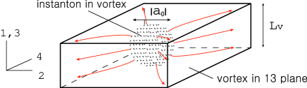
Figure 2: Single instanton in the Higgs phase. The size of the vortex is given by $L_{\rm v}\sim 1/g\sqrt{c}$.

Let us discuss the global structure (topology) of the the moduli space ${\cal M}^{1\text{-instanton}}$ of one instanton. The moduli matrix in one patch $H_{0}^{\prime}$ corresponding to the second one in Eq. (3.11) is related to that in the other patch $H_{0}$ in Eq.(3.47) by a world volume transformation $V$ as

$$H_{0}^{{}^{\prime}\text{1-instanton}}\equiv\sqrt{c}\left(\begin{array}[]{cc}\alpha^{\prime}(w-p^{\prime}_{1})+a^{\prime}&w-p^{\prime}_{1}\\ \alpha^{\prime}(z-z_{0})&z-z_{0}\end{array}\right)=VH_{0}^{\text{1-instanton}},\quad V=\left(\begin{array}[]{cc}0&1/\alpha\\ 1/\alpha&0\end{array}\right),$$ (3.53)

with the following relation between coordinates in two patches

$$\alpha^{\prime}=\frac{1}{\alpha},\quad a^{\prime}=-\frac{a}{\alpha^{2}},\quad p^{\prime}_{1}=p_{1}-\frac{a}{\alpha}.$$ (3.54)

Here both $\alpha$ and $\alpha^{\prime}$ are the patches of the standard inhomogeneous coordinates of the ${\mathbf{C}}P^{1}$ and they are enough to cover the whole manifold. We see that $p_{1}$ and $a$ transform in the union of the two patches $\alpha$ and $\alpha^{\prime}$. We find that $a$ requires a nontrivial transition function $-1/\alpha^{2}$ between two patches, showing that it is a tangent vector as a fiber on the ${\mathbf{C}}P^{1}$. However, instead of $p_{1}$ we can use the coordinate $p_{0}$ in Eq. (3.48) which is an invariant global coordinate for two patches, indicating that the space ${\bf C}$ parametrized by $p_{0}$ is a direct product to the ${\mathbf{C}}P^{1}$. Therefore we obtain the topology of the moduli space of one $U(2)$ instanton in the Higgs phase as

$$(z_{0},p_{0},a,\alpha)\in{\bf C}\times{\bf C}\times({\bf C}^{*}\ltimes{\bf C}P^{1})\simeq{\cal M}^{1\text{-instanton}},$$ (3.55)

with $F\ltimes B$ denoting a fiber bundle over a base space $B$ with a fiber $F$. More precisely ${\bf C}^{*}\ltimes{\bf C}P^{1}$ is the tangent bundle without zero section.

Here we make a comment on (non-)normalizability of zero modes. Some zero modes corresponding to these moduli parameters in (3.55) are not normalizable under four dimensional integration over the all codimensions. For instance the modulus $z_{0}$ for the position of the vortex is normalizable in two dimensions perpendicular to the vortex but is apparently non-normalizable in four dimensions. The modulus $\alpha$ parametrizes the boundary condition of the sigma model instanton in the effective theory on the vortex. It is also non-normalizable in the effective theory and therefore in the original theory. Nevertheless we emphasize that all of the moduli parameters in (3.55) are needed to determine the configuration of this composite state, and that dynamics of the composite state is described by these parameters.

For the case of $N>2$ we can specify the moduli matrix $H_{0}(z,w)$ for a particular class of $1/4$ BPS solutions identified as $1/2$ BPS states in the vortex theory, similarly to the case of $N=2$. We could also obtain the moduli matrices and the moduli space for $1/4$ BPS states corresponding to the $U(N)$ instantons in the Higgs phase by repeating the same discussion.

4 Monopoles and calorons in the Higgs phase

Recently, $1/4$ BPS states of the monopoles in the Higgs phase were studied [8]–[12] in $3+1$ dimensional massive SQCD with non-degenerate masses for hypermultiplets. Unlike the case of the massless model (or the massive model in which all the mass parameters are degenerate), the $SU(N_{\rm F})$ flavor symmetry is explicitly broken to $U(1)^{N_{\rm F}-1}$ in the massive case. Therefore vortices in the model with non-degenerate masses are essentially Abelian (ANO) vortices, and moduli fields corresponding to the orientational moduli paramters [9, 13, 25] are not exactly massless moduli in the effective theory of vortices. It has been found that the effective theory of the non-Abelian vortices can be constructed in the case where the mass difference is very smaller than the FI paramter $|\Delta m|\ll\hat{g}\sqrt{\hat{c}}$ [32, 8]. Here $\hat{g}$ and $\hat{c}$ are the gauge coupling and the FI parameter in 3+1 dimensions, respectively. The effective theory has a potential $\hat{V}\sim k^{2}$ where $k$ is a Killing vector on the moduli space of the non-Abelian vortices in the massless model[32, 8]. In the following of this section we call the vortex theory with the potential massive vortex theory and the vortex theory without any potential massless vortex theory.

It has been shown in Ref.[8] that the 1/4 BPS state of the monopoles in the Higgs phase can be realized as the 1/2 BPS kinks in the massive vortex theory (A${}^{\prime}\!\to$B${}^{\prime}\!\to$C^′ in Fig.1). In this section we will find the 1/4 BPS solution corresponding to the monopoles in the Higgs phase directly. Namely, we specify the moduli matrix for the 1/4 BPS state of the monopoles in the Higgs phase (A${}^{\prime}\!\to$C^′ in Fig.1). To achieve this, we find that it is very useful to promote the 3+1 dimensional massive theory to the 4+1 dimensional massless theory (A^′​$\to$A in Fig.1). By this procedure a monopole in 3+1 dimensions becomes a monopole-string in 4+1 dimensions. This 4+1 dimensional point of view (the triangle ABC in Fig.1) not only gives a nice realization of the monopoles but also leads to calorons in the Higgs phase which interporate between the instantons and the monopoles in the Higgs phase.

4.1 Walls, vortices and monopoles revisited

The four-dimensional massive model with non-degenerate masses

$$M\equiv{\rm diag.}(m_{1},m_{2},\cdots,m_{N_{\rm F}}),$$ (4.1)

for hypermultiplets can be derived from our five-dimensional massless SQCD by performing the Scherk-Schwarz (SS) dimensional reduction [27] (A$\to$A^′ in Fig.1), in which the fifth direction $x^{4}$ is compactified on $S^{1}$ with radius $R$ using a twisted boundary condition

$$H(x^{\mu},x^{4}+2\pi R)=H(x^{\mu},x^{4})e^{i2\pi RM},$$ (4.2)

with $0\leq m_{A}<1/R$. If we ignore the infinite towers of the Kaluza-Klein modes, we have the lightest mass field $\hat{H}(x^{\mu})$ as a function of the four-dimensional spacetime coordinates

$$H(x^{\mu},x^{4})=\frac{1}{\sqrt{2\pi R}}\hat{H}(x^{\mu})e^{iMx^{4}},$$ (4.3)

with $\mu=0,1,2,3$. Other fields neutral under the $SU(N_{\rm F})$ flavor symmetry are of the form

$$W_{\mu}(x^{\mu},x^{4})=W_{\mu}(x^{\mu}),\quad\Sigma(x^{\mu},x^{4})-iW_{4}(x^{\mu},x^{4})=\Sigma(x^{\mu})+i\hat{\Sigma}(x^{\mu}).$$ (4.4)

The $1/4$ BPS equations (we have ignored $H^{2}$ and $\Sigma$) in (2.8) and (2.9) reduce to those in four dimensions [22]

$$F_{12}=-\mathcal{D}_{3}\hat{\Sigma},\ F_{23}=-\mathcal{D}_{1}\hat{\Sigma},\ \bar{\mathcal{D}}_{z}\hat{H}=0,\ \mathcal{D}_{2}\hat{H}=\hat{H}M-\hat{\Sigma}\hat{H},$$ (4.5)

$$F_{13}-\mathcal{D}_{2}\hat{\Sigma}=-\frac{\hat{g}^{2}}{2}\left(\hat{c}{\bf 1}_{N_{\rm C}}-\hat{H}\hat{H}^{\dagger}\right).$$ (4.6)

Here the gauge coupling $\hat{g}$ and the FI paramter $\hat{c}$ in four dimensions are given by

$$\frac{1}{\hat{g}^{2}}\equiv\int^{2\pi R}_{0}dx^{4}\ \frac{1}{g^{2}}=\frac{2\pi R}{g^{2}},\qquad\hat{c}\equiv\int^{2\pi R}_{0}dx^{4}\ c=2\pi Rc,$$ (4.7)

respectively. It was known that these BPS equations admit walls, vortices and monopoles as $1/4$ BPS states [8, 22] (A${}^{\prime}\!\to$C^′ in Fig.1). The supercharges preserved by the above BPS equations are summarized in the Table 1:

Table 1: Gamma matrices of the projection operators for $1/4$ BPS states in 4 and 5 dimensions. Here we define $\gamma^{5}\equiv-i\gamma^{4}=i\gamma^{0}\gamma^{1}\gamma^{2}\gamma^{3}$. In our previous paper [22], we used another set of gamma matrices related by the redefinition $\gamma^{m}\to-\gamma^{m}i\gamma^{5}$, and chose the wall profile along $x^{3}$ instead of the present choice of $x^{2}$.

$d=4+1$ world-volume $\Gamma$ vortex 0,2,4 $-\gamma^{13}\otimes i\sigma^{3}$ vortex 0,1,3 $-\gamma^{24}\otimes i\sigma^{3}$ instanton 0 $\gamma^{0}\otimes{\bf 1}_{2}$

$d=3+1$ world-volume $\Gamma$ vortex 0,2 $-\gamma^{13}\otimes i\sigma^{3}$ wall 0,1,3 $-i\gamma^{2}\gamma^{5}\otimes i\sigma^{3}$ monopole 0 $\gamma^{0}\otimes{\bf 1}_{2}$

The Table 1 shows that vortices in the 1-3 plane, vortices in the 2-4 plane and instantons in five dimensions are the BPS states with the conserved supercharge specified by the same projection as vortices in the 1-3 plane, walls transverse to the $x^{2}$-direction and monopoles in four dimensions, respectively. Therefore after the SS dimensional reduction, these BPS solitons in five dimensions reduce to the respective BPS solitons in four dimensions. In fact, the instanton charge coincides with the monopole charge under the SS dimensional reduction as

$$\frac{1}{2g^{2}}\int d^{3}x\int^{2\pi R}_{0}dx^{4}\ {\rm Tr}(F_{mn}\tilde{F}^{mn})=\frac{2}{\hat{g}^{2}}\int d^{3}x\ \vec{\partial}\cdot{\rm Tr}(^{*}\!\vec{F}\hat{\Sigma}).$$ (4.8)

The BPS equations in Eqs.(4.5) and (4.6) in 3+1 dimensional massive theory have been solved in terms of the moduli matrix of the system [22]. Especially all the exact solutions were obtained in the strong gauge coupling limit $\hat{g}^{2}\to\infty$ in the semilocal case with $N_{\rm F}>N_{\rm C}$. Here we reconsider Eqs.(4.5) and (4.6) in general case of $N_{\rm F}\geq N_{\rm C}$ from the five-dimensional point of view. For that purpose, let us consider a restricted sector of the moduli space which is specified by the moduli matrix $H_{0}(z,w)$ in the form of

$$H_{0}(z,w)=\frac{1}{\sqrt{2\pi R}}\hat{H}_{0}(z)e^{Mw},$$ (4.9)

where an $N_{\rm C}\times N_{\rm F}$ matrix $\hat{H}_{0}(z)$ does not depend on $w,\bar{w}$, and is holomorphic with respect to $z$. The matrix $\hat{H}_{0}(z)$ should have rank $N_{\rm C}$ in generic points of $z$ (namely, apart from isolated points). Note that this restriction (4.9) is up to the world-volume transformation (2.14). For the restricted moduli matrix given above the “source” $\Omega_{0}$ of the master equation (2.17) is independent of the $x^{4}$-coordinate $\Omega_{0}(x^{M})=\hat{c}^{-1}\hat{H}_{0}e^{2Mx^{2}}\hat{H}_{0}^{\dagger}\equiv\hat{\Omega}_{0}(x^{\mu}).$ Then the solution $\Omega$ of Eq.(2.17) is also independendent of the $x^{4}$-coordinate: $S(x^{M})=\hat{S}(x^{\mu})$ and $\Omega(x^{M})=SS^{\dagger}=\hat{S}\hat{S}^{\dagger}\equiv\hat{\Omega}(x^{\mu}).$ At this stage, the master equation (2.17) reduces to

$$4\bar{\partial}_{z}\left(\partial_{z}\hat{\Omega}\hat{\Omega}^{-1}\right)+\partial_{2}\left(\partial_{2}\hat{\Omega}\hat{\Omega}^{-1}\right)=\hat{c}\hat{g}^{2}\left({\bf 1}_{N_{\rm C}}-\hat{\Omega}_{0}\hat{\Omega}^{-1}\right).$$ (4.10)

Their solution (2.12) can also be rewritten as follows

$$H=\frac{1}{\sqrt{2\pi R}}\hat{S}^{-1}\hat{H}_{0}e^{Mw},\quad\bar{W}_{z}=-i\hat{S}^{-1}\bar{\partial}_{z}\hat{S},\quad W_{2}-i\hat{\Sigma}=-i\hat{S}^{-1}\partial_{2}\hat{S}.$$ (4.11)

Notice that the above solution automatically satisfies the condition of the SS dimensional reduction (4.3) if we identify

$$\hat{H}(x^{\mu})=\hat{S}^{-1}(x^{\mu})\hat{H}_{0}(z)e^{Mx^{2}}.$$ (4.12)

The master equation (4.10) and its solutions (4.11) and (4.12) completely agree with those for the 1/4 BPS states containing walls, vortices and monopoles [22]. Therefore the restriction (4.9) to the form of the moduli matrix gives a map from 1/4 BPS solutions in 3+1 dimensions to those in 4+1 dimensions (C$\to$C^′ in Fig.1).

We now realize that all the 1/4 BPS states of the walls, vortices and monopoles in the massive SQCD [22] have one to one correspondence with those in the restricted sector (4.9) of our 1/4 BPS states (vortices and instantons) in the five-dimensional massless SQCD. The moduli space of the former can also be understood from the five-dimensional point of view as

$${\cal M}_{\rm wvm}={\cal H}_{\rm wvm}\backslash{\cal G}_{\rm wvm},$$ (4.13)

$${\cal G}_{\rm wvm}\equiv\{\hat{H}_{0}\ |\ {\bf C}{\longrightarrow}M(N_{\rm C}\times N_{\rm F},{\bf C}),\bar{\partial}_{z}\hat{H}_{0}=0\},$$

$${\cal H}_{\rm wvm}\equiv\{V\ |\ {\bf C}{\longrightarrow}GL(N_{\rm C},{\bf C}),\bar{\partial}_{z}V=0\},$$

where $\hat{H}_{0}(z)$ must have the maximal rank $N_{\rm C}$ in generic $z$ except for several points. It is interesting to observe that this total moduli space agree with that for the non-Abelian vortices in Eq.(3.2), $\cal{M}_{\rm wvm}\simeq{\cal M}_{\rm v}$, although the former is for 1/4 BPS states and the latter is for 1/2 BPS states. In the strong gauge coupling limit the moduli space ${\cal M}_{\rm wvm}$ becomes

$${\cal M}_{\rm wvm}^{g^{2}\rightarrow\infty}=\{\varphi|{\bf C}\rightarrow G_{N_{\rm F},N_{\rm C}},\bar{\partial}_{z}\varphi=0\},$$ (4.14)

in the case of $N_{\rm F}>N_{\rm C}$. This coincides with the moduli space of the Grassmannian sigma-model lumps [17] which can be classified by $\pi_{2}(G_{N_{\rm F},N_{\rm C}})={\bf Z}$ if we compactify ${\bf C}$ to ${\bf C}P^{1}$.

Moreover, if we push forward this descent relation from ${\cal M}_{\rm vv^{\prime}i}$ to ${\cal M}_{\rm wvm}$, we arrive at solutions of the non-Abelian walls and their moduli space ${\cal M}_{\rm w}$ which have been extensively studied in Ref.[30, 39]. To achieve this, we ignore $z$ dependence in ${\cal M}_{\rm wvm}$:

$${\cal M}_{\rm w}={\cal H}_{\rm w}\backslash{\cal G}_{\rm w}\simeq G_{N_{\rm F},N_{\rm C}},$$ (4.15)

$${\cal G}_{\rm w}\equiv\{\tilde{H}_{0}\ |\ {\bf C}^{0}{\longrightarrow}M(N_{\rm C}\times N_{\rm F},{\bf C}),{\rm rank}N_{\rm C}\}=\{M(N_{\rm C}\times N_{\rm F},{\bf C}),{\rm rank}N_{\rm C}\},$$

$${\cal H}_{\rm w}\equiv\{V\ |\ {\bf C}^{0}{\longrightarrow}GL(N_{\rm C},{\bf C})\}=GL(N_{\rm C},{\bf C}),$$

where ${\bf C}^{0}$ is just a point. The condition on the constant matrix $\tilde{H}_{0}$ to have the maximal rank $N_{\rm C}$ has been deduced from the condition on $H_{0}(z,w)$ or $\hat{H}_{0}(z)$ in generic points of $z$ or $(z,w)$ in the case of instantons or monopoles, respectively. It comes from the fact that the moduli matrix must have rank $N_{\rm C}$ in the vacuum. It is interesting that in the strong gauge coupling $(N_{\rm F}>N_{\rm C})$ the total moduli space is unchanged

$${\cal M}_{\rm w}^{g^{2}\rightarrow\infty}\simeq{\cal M}_{\rm w},$$ (4.16)

unlike the case of other solitons because the moduli matrix $\tilde{H}_{0}$ is a constant matrix here.

We thus have found that solutions of our BPS equations (2.8) and (2.9) can give all four kinds of solitons: walls, vortices, monopoles and instantons. The relations between their total moduli spaces are given by

$${\cal M}_{\rm w}\subset{\cal M}_{\rm wvm}\left(\simeq{\cal M}_{\rm v}\right)\subset{\cal M}_{\rm vv^{\prime}i}.$$ (4.17)

4.2 Monopoles in the Higgs phase

Let us next find the solution of Eqs.(4.5) and (4.6) (A${}^{\prime}\!\to$C^′ in Fig.1) corresponding to one monopole in the Higgs phase, namely a single monopole attatched to a vortex. To be precise, we restrict ourselves into the simplest case with $N_{\rm C}=N_{\rm F}\equiv N=2$ in the following of this section. As was explained in Sec. 3, the most general moduli matrix containing a single vortex can be written in the form of

$$\hat{H}_{0}(z)=\sqrt{\hat{c}}\left(\begin{array}[]{cc}z-z_{0}&0\\ b_{c}&1\end{array}\right),$$ (4.20)

where $b_{c}$ is a constant complex paramter. Notice that this is the same form with the moduli matrix (3.11) generating only a single vortex in the massless theory. However in the massive theory the moduli matrix (4.20) gives not only a vortex but also a monopole, where $b_{c}$ gives the position and the phase of a monopole inside the vortex, as will be shown below. The difference between the massless theory and the massive theory appears as the factor $e^{Mx^{2}}$ in Eq. (4.12) which is absent in Eq.(2.12). In the massless limit $M\to 0$, the moduli matrix (4.20) gives a single vortex only as expected.

Similarly to instantons in the Higgs phase, we can calculate charge of the monopole in the Higgs phase in terms of the massive vortex theory. To this end, let us recall the following two facts. One is that the instantons can be realized as lumps in the massless vortex theory with the Kähler potential (3.22) (A$\to$B$\to$C in Fig.1). The other is that 1/4 BPS states in the four-dimensional massive theory can be obtained by the restriction (4.9) on 1/4 BPS states in the five-dimensional massless theory (C$\to$C^′ in Fig.1). Combining these facts together, we naturally arrive at a notion of the SS dimensional reduction for the vortex theory (B$\to$B^′ in Fig.1). In order to achieve this, we should first find what the action of the SS dimensional reduction to the vortex theory is. In terms of the moduli matrix $H_{0}(z,w)$ the above twisted boundary condition (4.2) can be translated in terms of the moduli matrix as $H_{0}(z,w+2\pi iR)=VH_{0}(z,w)e^{2\pi iRM}$ where $V(z,w)$ is an element of world-volume transformation (2.14). This naturally induces the following twisted boundary condition on the moduli fields $z_{0}(t,x^{2},x^{4})$ and $b(t,x^{2},x^{4})$ in the moduli matrix $H_{{\rm v}0}^{\rm single}(z;z_{0},b)$ in the effective theory of the host vortex

$$H_{{\rm v}0}^{\rm single}\left(z;z_{0}(t,x^{2},x^{4}+2\pi R),b(t,x^{2},x^{4}+2\pi R)\right)$$

$$=VH_{{\rm v}0}^{\rm single}\left(z;z_{0}(t,x^{2},x^{4}),b(t,x^{2},x^{4})\right)e^{i2\pi RM},$$ (4.21)

with $V=e^{-2\pi iRM}$. Hence we can identify the twisted boundary condition to the moduli fields as $z_{0}(t,x^{2},x^{4}+2\pi R)=z_{0}(t,x^{2},x^{4})$ and $b(t,x^{2},x^{4}+2\pi R)=e^{i2\pi R\Delta m}b(t,x^{2},x^{4})$ with $\Delta m\equiv m_{1}-m_{2}$. We thus get the action of the SS dimensional reduction for $z_{0}$ and $b$ as

$$z_{0}(t,x^{2},x^{4})=\hat{z}_{0}(t,x^{2}),\quad b(t,x^{2},x^{4})=e^{i\Delta mx^{4}}\hat{b}(t,x^{2}).$$ (4.22)

Plugging (4.22) into the effective Lagrangian with the Kähler potential (3.22) of the 2+1 dimensional massless vortex theory, we can obtain the effective Lagrangian for the massive vortex thoery after integrating over $x^{4}$ (B$\to$B^′ in Fig.1). The resulting 1+1 dimensional massive vortex theory consists of the scalar potential $\hat{V}_{\rm v}$ arising from the kinetic term in extra dimension $x^{4}$ and the Kähler potential $\hat{K}_{\rm v}$, given by

$$\hat{K}_{\rm v}=\hat{c}\pi|\hat{z}_{0}|^{2}+\frac{4\pi}{\hat{g}^{2}}\log\left(1+|\hat{b}|^{2}\right),\quad\hat{V}_{\rm v}=\frac{4\pi}{\hat{g}^{2}}\frac{\Delta m^{2}|\hat{b}|^{2}}{\left(1+|\hat{b}|^{2}\right)^{2}}.$$ (4.23)

These exactly agree with the results in Ref.[8] including the Kähler class of the Kähler potential and the coefficient of the scalar potential.

The scalar potential in Eq.(4.23) admits two discrete SUSY vacua at $\hat{b}=0,\infty$. Thus $1/2$ BPS states on the vortex theory become kinks (B${}^{\prime}\!\to$C^′ in Fig.1). In fact, the $1/2$ BPS equation (3.4) reduces to

$$\partial_{2}\hat{b}-\Delta m\hat{b}=0,$$ (4.24)

and the solution interpolating between $\hat{b}=0$ and $\hat{b}=\infty$ is found to be

$$\hat{b}(t,x^{2})=e^{-i\theta}e^{\Delta m(x^{2}-x^{2}_{0})},$$ (4.25)

where $e^{-i\theta}$ is a phase and a real parameter $x^{2}_{0}$ is a position of the kink [26]. Although this configuration exponentially grows, the energy density is localized around $x^{2}=x^{2}_{0}$

$${\cal E}=\frac{4\pi}{g^{2}}\frac{\Delta m^{2}}{\cosh^{2}\Delta m(x^{2}-x^{2}_{0})},$$ (4.26)

implying usual wall profile in suitable coordinates. The mass of the kink can be obtained by integrating this over the $x^{2}$-coordinate and we get $4\pi\Delta m/\hat{g}^{2}$. This coincides with the mass of a monopole in the Coulomb phase. Thus monopoles in the Higgs phase can be seen as the $1/2$ BPS kinks in the vortex theory[8].

Before closing this subsection, let us clarify the relation between $b_{c}$ in the moduli matrix (4.20) and $\theta$ and $x^{2}_{0}$ in the 1/2 BPS kink solution (4.25). For that purpose the five-dimensional point of view (triangle ABC in Fig.1) gives us a very nice picture. Taking Eq.(4.22) into account, the monopole(kink) solution (4.25) is understood in the massless vortex theory (3.22) as ((B${}^{\prime}\!\to$C^′)$\to$(B$\to$C) in Fig.1)

$$b(t,x^{2},x^{4})=e^{i\Delta mx^{4}}\hat{b}(t,x^{2})=e^{-(\Delta mx^{2}_{0}+i\theta)}e^{\Delta mw}.$$ (4.27)

Note that the Kähler potential (3.22) with this solution substituted is independent of $x^{4}$ because it is a function of $|b|=e^{\Delta m(x^{2}-x^{2}_{0})}$. Therefore the energy density of this configuration extends along the $x^{4}$-axis to infinity. Then this configuration is understood as a 1/4 BPS state of the monopole-string in the Higgs phase. Let us next find the moduli matrix $H_{0}(z,w)$ in five dimensions corresponding to the moduli matrix given in Eq.(4.20) for the monopole in the Higgs phase in four dimensions. This can be obtained from the first equation in Eq.(4.11) with $S(x^{M})=\hat{S}(x^{\mu})$ as ((A${}^{\prime}\!\to$C^′)$\to$(A$\to$C) in Fig.1)

$$H_{0}(z,w)=\sqrt{c}\left(\begin{array}[]{cc}z-z_{0}&0\\ b(w)&1\end{array}\right)=\sqrt{c}\ V\left(\begin{array}[]{cc}z-z_{0}&0\\ b_{c}&1\end{array}\right)e^{Mw},\quad V=e^{-Mw}.$$ (4.32)

We thus find $b(w)=b_{c}e^{\Delta mw}$. Comparing this with the kink solution in (4.27), the complex parameter $b_{c}$ can be identified as ((A$\to$C) = (A$\to$B$\to$C) in Fig.1)

$$b_{c}=e^{-(\Delta mx_{0}^{2}+i\theta)}.$$ (4.33)

Hence, we conclude that the 1/4 BPS moduli matrix (4.20) describes a monopole in the Higgs phase and the complex parameter $b_{c}$ therein is the position and the phase of the monopole. In the massless limit $\Delta m\to 0$ with $\Delta mx^{2}_{0}$ fixed, $b_{c}$ becomes the orientational moduli of the non-Abelian vortex since the $SU(2)_{\rm F}$ flavor symmetry, which is explicitly broken to $U(1)_{\rm F}$ by non-zero $\Delta m$, is restored when $\Delta m=0$.

4.3 Calorons in the Higgs phase

In the Coulomb phase (unbroken gauge symmetry) there is well known way to get ordinary monopole solution independent of $x^{4}$ from instanton solutions[28, 29]. Range the instantons with equal size along the $x^{4}$-axis periodically. After takeing the limit where the size parameter of instantons goes to infinity the configuration becomes one BPS monopole-string solution extending to the $x^{4}$-axis[28, 29]. In the Higgs phase, instantons, a monopole-string and calorons which interpolate between instantons and the monopole-string can be understood in terms of the deformations of the lump solutions in the vortex theory. In this subsection we will concentrate on 1/2 BPS states in the 2+1 dimensional massless vortex theory with the Kähler potential (3.22) (B$\to$C in Fig.1).

Let us first examine the monopole-string solution (4.27) as the sigma model lump in the massless vortex theory in more detail. We first note that the solution $b=b_{c}e^{\Delta mw}$ in Eq.(4.27) is a 1/2 BPS state in the vortex theory since this is holomorphic in $w$ and is a solution of the BPS equation (3.4) in the vortex theory. Although this solution has one co-dimension in the vortex theory, this is not a domain wall which is a topological soliton supported by the homotopy group $\pi_{0}$ because there is no scalar potential here. Rather, we should realize this soution as a topological object which consists of an infinite number of 1/2 BPS lumps supported by the homotopy group $\pi_{2}$. To see this, we decompose the solution as $b=b_{c}e^{\Delta mx^{2}}e^{i\Delta mx^{4}}$. Then it is clear that a strip $\sigma_{\rm l}^{(k)}=\{(x^{2},x^{4})\ |\ x^{2}\in(-\infty,\infty),\ x^{4}\in[2\pi k/\Delta m,2\pi(k+1)/\Delta m]\}$ is mapped to the ${\bf C}P^{1}$ manifold once by this configuration. Then the solution $b=b_{c}e^{\Delta mw}$ has infinite winding number $\pi_{2}({\bf C}P^{1})=\infty$. Hence this can be realized as topological object which has an infinite number of lump charge. The energy density of the solution is the same form as that in Eq.(4.26). If we integrate this in a strip $\sigma^{(k)}_{\rm m}=\{(x^{2},x^{4})\ |\ x^{2}\in(-\infty,\infty),\ x^{4}\in[2\pi kR,2\pi(k+1)R]\}$ ($R$ is a compactification radius associated with the SS dimensional reduction), we find that the tension of the solution in the strip $\sigma_{\rm m}^{(k)}$ coincides with to the mass of the monopole $4\pi\Delta m/\hat{g}^{2}$. So this solution is suitable to be called the monopole-string.

Let us next consider 1/4 BPS calorons in the Higgs phase.

$$b(w)=\left(1+\theta\right)e^{\mu(w-w_{0})}-\theta,\qquad\theta\equiv\frac{1}{a\mu}.$$ (4.34)

Here, $\mu$ and $a$ are arbitrary real parameters with mass dimension one and minus one respectively.

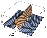
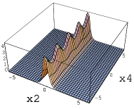
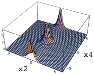
(a) monopole-string	(b) caloron	(c) caloron	(d) instanton
$\mu=2,\ \theta=5\times 10^{-4}$	$\mu=2,\ \theta=0.1$	$\mu=1,\ \theta=1$	$\mu=0.2,\ \theta=5$

Figure 3: Energy density of the calorons in terms of the vortex theory.

Similarly to the ordinary calorons in the Coulomb phase[28, 29], the calorons in the Higgs phase can be continuously deformed the monopole-string or instantons. In fact, in the limit $\theta\rightarrow 0$ with $\mu$ fixed, this solution reduces to the 1/4 BPS monopole-string $b\rightarrow e^{\mu(w-w_{0})}$ as shown in Fig.3(a). There is an another limit $\theta\to\infty$ with $a$ fixed. In this limit this solution reduces to $1/4$ BPS states of an instanton in the Higgs phase as shown in Fig.3(d). For general $\theta$, we find periodic lump solutions inside a vortex which can be understood as the 1/4 BPS caloron as shown in Fig.3(b) and (c). The parameter $a$ is the size of the instanton and $1/\mu$ is the period of the caloron.

In view of this solution, we can guess that the monopole strings with large instanton charges in the compactified theory are unstable as follows. If we compactify the $x^{4}$-direction with radius $R$, the mass of the monopole-string solution $b=e^{\mu(w-w_{0})}$ is $8\pi^{2}R\mu/g^{2}$. To be precise, let us represent $\mu=(k+\tau)/R$ with $k\in{\bf Z}$ and $\tau\in[0,1)$. Then the above mass of the monopole-string can be rewritten as

$$\frac{8\pi^{2}}{g^{2}}k+\frac{4\pi}{\hat{g}^{2}}\Delta m,\quad\left(\frac{\tau}{R}\equiv\Delta m\right).$$ (4.35)

This mass corresponds to the mass of $k$-instantons and a monopole with a “fractional” instanton charge $\tau$. Then the monopole-string with mass $8\pi^{2}R\mu/g^{2}$ can be decomposed into these solitons by continuous deformation like (4.34). Since the aggregate of the decomposed solitons has larger entropy, the monopole-string with instanton charge greater than unity is unstable and may decay into instantons and a monopole-string with the fractional instanton charge, if this system is put at finite tempertures.

5 Conclusion and Discussion

We have solved $1/4$ BPS equations for composite states made of instantons and vortices. We have shown that all solutions are generated by the moduli matrix which is a holomorphic function of $z=x^{1}+ix^{3}$ and $w=x^{2}+ix^{4}$. The moduli matrix contains all solutions with different boundary conditions and/or different topological charges. As a first step toward the complete classification of all solutions, we have specified the moduli matrix for $1/4$ BPS states which can be interpreted as lumps on a single vortex. Small instanton singularities have been shown to correspond to small lump singularities. We have determined the moduli space for a single instanton in the Higgs phase to be the direct product of ${\bf C}^{2}$ and the tangent bundle over ${\bf C}P^{1}$ without zero section. We have clarified the relations between the moduli spaces of 1/4 BPS states for vortices and instantons, of 1/4 BPS states for walls, vortices and monopoles, of 1/2 BPS vortices, and of 1/2 BPS walls. We also have constructed calorons in the Higgs phase which interpolate between instantons and a monopole-string in the Higgs phase.

We did not exhaust all solutions in this paper: our moduli matrix contains more varieties of solutions. The complete classification of all solutions is a very important open problem. Let us discuss this issue. First of all we could consider multiple vortices as host solitons. However the moduli matrix for multiple vortices is not available yet. It is now in progress to specify the moduli parameters in the moduli matrix, and therefore we have to wait for the completion of that work [38] to discuss the multiple lumps on multiple vortices.

Second, if we do not restrict ourselves to solitons which can be understood as lumps on vortices, we can obtain more varieties of solitons. Intersection of two or more vortices cannot be understood as solitons in the effective theory on a host vortex, because the energy of such solitons diverges in the effective theory in general. Instead, we can directly construct solutions of intersecting vortices as follows. In the same model with $N=2$, the following two moduli matrices give configurations with $\nu_{\rm v}=k_{z}(\geq 0)$ vortices in the 1-3 plane and $\nu_{\rm v^{\prime}}=k_{w}(\geq 0)$ vortices in the 2-4 plane

$$H_{0}=\left(\begin{array}[]{cc}z^{k_{z}}&0\\ 0&w^{k_{w}}\end{array}\right),\quad\quad H_{0}=\left(\begin{array}[]{cc}z^{k_{z}}w^{k_{w}}&0\\ 0&1\end{array}\right).$$ (5.5)

The vortices intersect at a point for both cases. It is, however, a trivial intersection for the former case, and they carry no instanton charge. On the other hand, they intersect non-trivially for the latter case, and the intersecting point carries the instanton charge $\nu_{\rm i}=-k_{z}k_{w}$. In this case the instantons give a negative energy contribution. However, there is no inconsistency, since the total energy including vortices is always positive. Since the instanton is stuck at the intersecting point of vortices, it may be called an “intersecton”. It cannot move once the vortices are fixed. We thus conclude that there exist two kinds of instantons; one is what lives inside a vortex and the other is an instanton stuck at the intersection point of vortices. As we have seen, there also exists trivially intersecting vortices. We expect that the most general solution is given by the mixture of these configurations.

Here we show that the intersectons found above essentially exist in $U(1)$ gauge theories. To this end we consider multiple semilocal vortices in the theory with $N_{\rm F}>N_{\rm C}$. We take the strong gauge coupling limit $g^{2}\rightarrow\infty$ to obtain an exact solution. In this limit the model reduces to a nonlinear sigma model whose target space is the cotangent bundle over the complex Grassmann manifold, $T^{*}(G_{N_{\rm F},N_{\rm C}})$ [36]. Then the master equation (2.17) can be solved algebraically as Eq. (2.23). For definiteness we consider a model with $N_{\rm C}=1$ and $N_{\rm F}=4$. The following moduli matrix gives non-trivially intersecting vortices with $\nu_{\rm v}=k_{z},\ \nu_{\rm v^{\prime}}=k_{w}$

$$H_{0}=\left(z^{k_{z}}w^{k_{w}},\ z^{k_{z}},\ w^{k_{w}},\ 1\right).$$ (5.6)

The $\Omega$ can be calculated as

$$\Omega^{g\to\infty}=\Omega_{0}=(|z|^{2}+1)^{k_{z}}(|w|^{2}+1)^{k_{w}}\;$$ (5.7)

and the exact solution can be obtained as $H=(1/\sqrt{\Omega^{g\to\infty}})H_{0}$. The instanton number can be calculated to be the product of vorticities, namely $\nu_{\rm i}=-k_{z}k_{w}$. This solution explicitly shows that the $U(1)$ instantons are stuck at the intersection of vortices. We can show that the instanton charge $\nu_{\rm i}$ changes its sign under the duality transformation $N_{\rm C}$, $\tilde{N}_{\rm C}\equiv N_{\rm F}-N_{\rm C}$ [30]. Therefore, there also exist intersectons with positive instanton charges.

We discuss some more issues in the following. Although we ignore $\Sigma$ and zero-th component of gauge potential $W_{0}$ in this paper, we can also construct electrically charged solitons whose charge is $Q_{e}=(g^{2}/2)\int d^{4}x\ \partial_{m}(\Sigma F_{0m})$ by restoring these fields. The Bogomol’nyi completion gives the most general BPS equations

$$\mathcal{D}_{0}\Sigma=0,\quad F_{m0}+\mathcal{D}_{m}\Sigma=0,\quad\mathcal{D}_{0}H^{i}+i\Sigma H^{i}=0,$$ (5.8)

added to Eq.(2.8) and (2.9). These equations have to be solved with the Gauss’s law

$$\frac{1}{g^{2}}\mathcal{D}_{m}F_{m0}=\frac{i}{g^{2}}\left[\Sigma,\mathcal{D}_{0}\Sigma\right]+\frac{i}{2}\left[H\mathcal{D}_{0}H^{\dagger}-\mathcal{D}_{0}HH^{\dagger}\right].$$ (5.9)

We can show that solutions of these equations are $1/4$ BPS states. If we turn off the FI paramter $c$ and set $H^{i}=0$, these BPS solutions reduces to that for the 1/2 BPS dyonic instanton[43]. The time-independent solutions of the dyonic instantons in the Higgs phase can be obtained as follows. First we solve the BPS equations (2.8) and (2.9) as shown in this paper. Next we set $\partial_{0}=0$ and $W_{0}=-\Sigma$ to solve additional equations (5.8). Finally $\Sigma$ can be obtained by solving the Gauss’s law under a given solution of instantons in the Higgs phase as the background

$$\mathcal{D}_{m}\mathcal{D}_{m}\Sigma=-\frac{g^{2}}{2}\left(HH^{\dagger}\Sigma+\Sigma HH^{\dagger}\right).$$ (5.10)

In superstring theory dyonic instantons in the pure SUSY Yang-Mills theory were found to be supertubes [44] (and see also references in [45]) between parallel D4-branes [46]. Brane constructions for the dyonic instantons in the Higgs phase is an open problem.

Our instantons in the Higgs phase share some properties with non-commutative instantons. First $U(1)$ instantons can exist in the Higgs phase as shown in Eq. (5.6) like non-commutative $U(1)$ instantons [20]. Second their topologies are similar (but not identical) as stated in the footnote 14. The moduli space of (non-commutative) instantons has the hyper-Kähler structure. Although the moduli space of the former has the Kähler structure at least and has real dimensions four multiplied by ${\bf Z}$, we do not know if it has the hyper-Kähler structure. It may be not the case because there remain only two SUSY in the former, but their moduli space may be obtained as a deformation of the moduli space of the latter preserving only the Kähler structure. It is very interesting to explore more simiralities between instantons in the Higgs phase and non-commutative instantons [20]. It is also desired to obtain the ADHM construction for our instantons in the Higgs phase.

Dynamics of instantons within a vortex is equivalent to the dynamics of lumps [14, 15]. Further studys in dynamics of sigma model lumps would clarify dynamics of instantons in more general configurations. Not only classical dynamics but also quantum effects in these solitons are important subjects. It was found by N. Dorey in [47] that the BPS spectra in $d=4$ ${\cal N}=2$ SUSY gauge theory with $N_{\rm F}>N_{\rm C}$ and $d=2$ ${\cal N}=(2,2)$ SUSY ${\bf C}P^{N}$ model with twisted masses completely coincide. One explanation for this coincidence has been given in [13, 10] by considering a monopole inside a vortex. In conformity with these observations, there exist similarities between $d=4$ Yang-Mills instantons and $d=2$ sigma-model instantons (lumps). Our results in the present paper give a further evidence for the relation because we have realized instantons inside a vortex as sigma model lumps on the vortex theory. For instance, small instanton singularities are understood as small lump singularities. It is also quite interesting to generalize the instanton couting [21] to the case of the instantons in the Higgs phase.

Non-Abelian walls found in [30] are recently realized as D-brane configurations in string theory [39]. By doing this the diverse phenomena of non-Abelian walls can be easily understood by dynamics of D-branes. Monopoles in the Higgs phase are also realized by the same brane configuration [13, 11]. Hence we would like to realize the instantons in the Higgs phase by some D-brane configuration, and we expect that the relation between monopoles and instantons in the Higgs phase can be interpreted as a T-duality in such a D-brane configuration, as in the case of the ordinary monopoles and instantons.

References

- [1] A. A. Belavin, A. M. Polyakov, A. S. Schwartz and Y. S. Tyupkin, Phys. Lett. B 59, 85 (1975).
- [2] M. F. Atiyah, N. J. Hitchin, V. G. Drinfeld and Y. I. Manin, Phys. Lett. A 65, 185 (1978).
- [3] I. Affleck, M. Dine and N. Seiberg, Nucl. Phys. B 241, 493 (1984).
- [4] N. Seiberg and E. Witten, Nucl. Phys. B 426, 19 (1994) [Erratum-ibid. B 430, 485 (1994)] [arXiv:hep-th/9407087]; Nucl. Phys. B 431, 484 (1994) [arXiv:hep-th/9408099]; N. Seiberg, Nucl. Phys. B 435, 129 (1995) [arXiv:hep-th/9411149].
- [5] I. Affleck, Nucl. Phys. B191, 429 (1981).
- [6] G. H. Derrick, J. Math. Phys. 5, 1252 (1964).
- [7] N. Manton and P. Sutcliffe, page 85, “Topological solitons”, Cambridge Univ. Press, (2004).
- [8] D. Tong, Phys. Rev. D 69, 065003 (2004) [arXiv:hep-th/0307302].
- [9] R. Auzzi, S. Bolognesi, J. Evslin and K. Konishi, Nucl. Phys. B 686, 119 (2004) [arXiv:hep-th/0312233].
- [10] M. Shifman and A. Yung, Phys. Rev. D 70, 045004 (2004) [arXiv:hep-th/0403149].
- [11] R. Auzzi, S. Bolognesi and J. Evslin, JHEP 0502, 046 (2005) [arXiv:hep-th/0411074].
- [12] M. A. C. Kneipp and P. Brockill, Phys. Rev. D 64, 125012 (2001) [arXiv:hep-th/0104171]; M. A. C. Kneipp, Phys. Rev. D 68, 045009 (2003) [arXiv:hep-th/0211049]; Phys. Rev. D 69, 045007 (2004) [arXiv:hep-th/0308086]; arXiv:hep-th/0401234.
- [13] A. Hanany and D. Tong, JHEP 0404, 066 (2004) [arXiv:hep-th/0403158].
- [14] R. S. Ward, Phys. Lett. B 158, 424 (1985).
- [15] I. Stokoe and W. J. Zakrzewski, Z. Phys. C 34, 491 (1987).
- [16] A. M. Polyakov and A. A. Belavin, JETP Lett. 22, 245 (1975) [Pisma Zh. Eksp. Teor. Fiz. 22, 503 (1975)].
- [17] A. M. Perelomov, Phys. Rept. 146, 135 (1987).
- [18] E. Witten, Nucl. Phys. B460, 541 (1996) [arXiv:hep-th/9511030]; M. R. Douglas, arXiv:hep-th/9512077.
- [19] P. B. Kronheimer and H. Nakajima, Math. Ann. 288, 263 (1990); H. Nakajima, Duke Math. J. 76, 365 (1994).
- [20] N. Nekrasov and A. Schwartz, Commun. Math. Phys. 198, 689 (1998) [arXiv:hep-th/9802068]; K. Furuuchi, Prog. Theor. Phys. 103, 1043 (2000) [arXiv:hep-th/9912047].
- [21] N. A. Nekrasov, Adv. Theor. Math. Phys. 7, 831 (2004) [arXiv:hep-th/0206161].
- [22] Y. Isozumi, M. Nitta, K. Ohashi and N. Sakai, Phys. Rev. D 71, 065018 (2005) [arXiv:hep-th/0405129].
- [23] A. Hanany and D. Tong, JHEP 0307, 037 (2003) [arXiv:hep-th/0306150].
- [24] R. Auzzi, S. Bolognesi, J. Evslin, K. Konishi and A. Yung, Nucl. Phys. B 673, 187 (2003) [arXiv:hep-th/0307287].
- [25] M. Eto, M. Nitta and N. Sakai, Nucl. Phys. B 701, 247 (2004) [arXiv:hep-th/0405161].
- [26] E. Abraham and P. K. Townsend, Phys. Lett. B 291, 85 (1992); J. P. Gauntlett, D. Tong and P. K. Townsend, Phys. Rev. D64, 025010 (2001) [arXiv:hep-th/0012178]; D. Tong, Phys. Rev. D66, 025013 (2002) [arXiv:hep-th/0202012]; JHEP 0304, 031 (2003) [arXiv:hep-th/0303151]; M. Arai, M. Naganuma, M. Nitta, and N. Sakai, Nucl. Phys. B652, 35 (2003) [arXiv:hep-th/0211103]; “BPS Wall in N=2 SUSY Nonlinear Sigma Model with Eguchi-Hanson Manifold” in Garden of Quanta - In honor of Hiroshi Ezawa, Eds. by J. Arafune et al. (World Scientific Publishing Co. Pte. Ltd. Singapore, 2003) pp 299-325, [arXiv:hep-th/0302028]; M. Arai, E. Ivanov and J. Niederle, Nucl. Phys. B 680, 23 (2004) [arXiv:hep-th/0312037].
- [27] J. Scherk and J. H. Schwarz, Nucl. Phys. B 153, 61 (1979).
- [28] B. J. Harrington and H. K. Shepard, Phys. Rev. D 17, 2122 (1978) ; P. Rossi, Nucl. Phys. B 149, 170 (1979); D. J. Gross, R. D. Pisarski and L. G. Yaffe, Rev. Mod. Phys. 53, 43 (1981); A. Actor, Annals Phys. 148, 32 (1983); A. Chakrabarti, Phys. Rev. D 35, 696 (1987).
- [29] K. M. Lee and P. Yi, Phys. Rev. D 56, 3711 (1997) [arXiv:hep-th/9702107]; K. M. Lee, Phys. Lett. B 426, 323 (1998) [arXiv:hep-th/9802012]; T. C. Kraan and P. van Baal, Phys. Lett. B 428, 268 (1998) [arXiv:hep-th/9802049]; Nucl. Phys. B 533, 627 (1998) [arXiv:hep-th/9805168]; Phys. Lett. B 435, 389 (1998) [arXiv:hep-th/9806034]; K. M. Lee and S. H. Yi, Phys. Rev. D 67, 025012 (2003) [arXiv:hep-th/0205274]; R. S. Ward, Phys. Lett. B 582, 203 (2004) [arXiv:hep-th/0312180].
- [30] Y. Isozumi, M. Nitta, K. Ohashi and N. Sakai, Phys. Rev. Lett. 93, 161601 (2004) [arXiv:hep-th/0404198]; Phys. Rev. D 70, 125014 (2004) [arXiv:hep-th/0405194].
- [31] Y. Isozumi, M. Nitta, K. Ohashi and N. Sakai, to appear in the proceedings of 12th International Conference on Supersymmetry and Unification of Fundamental Interactions (SUSY 04), Tsukuba, Japan, 17-23 Jun 2004 [arXiv:hep-th/0409110]; to appear in the proceedings of “NathFest” at PASCOS conference, Northeastern University, Boston, Ma, August 2004 [arXiv:hep-th/0410150].
- [32] D. Tong, Phys. Lett. B 460, 295 (1999) [arXiv:hep-th/9902005].
- [33] M. Eto, Y. Isozumi, M. Nitta, K. Ohashi, K. Ohta, N. Sakai and Y. Tachikawa, Phys. Rev. D (in press) [arXiv:hep-th/0503033].
- [34] N. S. Manton, Phys. Lett. B 110, 54 (1982).
- [35] T. Vachaspati and A. Achucarro, Phys. Rev. D 44, 3067 (1991) ; M. Hindmarsh, Phys. Rev. Lett. 68, 1263 (1992); G. W. Gibbons, M. E. Ortiz, F. Ruiz Ruiz and T. M. Samols, Nucl. Phys. B 385, 127 (1992) [arXiv:hep-th/9203023]; J. Preskill, Phys. Rev. D 46, 4218 (1992) [arXiv:hep-ph/9206216]; M. Hindmarsh, Nucl. Phys. B 392, 461 (1993) [arXiv:hep-ph/9206229]; A. Achucarro and T. Vachaspati, Phys. Rept. 327, 347 (2000) [arXiv:hep-ph/9904229].
- [36] U. Lindström and M. Roček, Nucl. Phys. B 222, 285 (1983); M. Arai, M. Nitta and N. Sakai, Prog. Theor. Phys. 113, 657 (2005) [arXiv:hep-th/0307274]; to appear in the Proceedings of the 3rd International Symposium on Quantum Theory and Symmetries (QTS3), September 10-14, 2003, [arXiv:hep-th/0401084]; to appear in the Proceedings of the International Conference on “Symmetry Methods in Physics (SYM-PHYS10)” held at Yerevan, Armenia, 13-19 Aug. 2003 [arXiv:hep-th/0401102]; to appear in the Proceedings of SUSY 2003 held at the University of Arizona, Tucson, AZ, June 5-10, 2003 [arXiv:hep-th/0402065].
- [37] A. A. Abrikosov, Sov. Phys. JETP 5, 1174 (1957) [Zh. Eksp. Teor. Fiz. 32, 1442 (1957)], [Reprinted in Solitons and Particles, Eds. C. Rebbi and G. Soliani (World Scientific, Singapore, 1984), p. 356]; H. B. Nielsen and P. Olesen, Nucl. Phys. B61, 45 (1973), [Reprinted in Solitons and Particles, Eds. C. Rebbi and G. Soliani (World Scientific, Singapore, 1984), p. 365].
- [38] M. Eto, Y. Isozumi, M. Nitta, K. Ohashi and N. Sakai, in preparation.
- [39] M. Eto, Y. Isozumi, M. Nitta, K. Ohashi, K. Ohta and N. Sakai, “D-brane Construction for Non-Abelian Walls,” [arXiv:hep-th/0412024].
- [40] M. Naganuma, M. Nitta and N. Sakai, Grav. Cosmol. 8, 129 (2002) [arXiv:hep-th/0108133]; R. Portugues and P. K. Townsend, JHEP 0204, 039 (2002) [arXiv:hep-th/0203181].
- [41] H. Oda, K. Ito, M. Naganuma and N. Sakai, Phys. Lett. B 471, 140 (1999) [arXiv:hep-th/9910095].
- [42] K. Ito, M. Naganuma, H. Oda and N. Sakai, Nucl. Phys. B 586, 231 (2000) [arXiv:hep-th/0004188]; Nucl. Phys. Proc. Suppl. 101, 304 (2001) [arXiv:hep-th/0012182]; M. Naganuma, M. Nitta and N. Sakai, Phys. Rev. D 65, 045016 (2002) [arXiv:hep-th/0108179]; in the proceedings of 3rd International Sakharov Conference On Physics, 24-29 Jun 2002, Moscow, Russia [arXiv:hep-th/0210205].
- [43] N. D. Lambert and D. Tong, Phys. Lett. B 462, 89 (1999) [arXiv:hep-th/9907014]; M. Zamaklar, Phys. Lett. B 493, 411 (2000) [arXiv:hep-th/0006090]; E. Eyras, P. K. Townsend and M. Zamaklar, JHEP 0105, 046 (2001) [arXiv:hep-th/0012016].
- [44] D. Mateos and P. K. Townsend, Phys. Rev. Lett. 87, 011602 (2001) [arXiv:hep-th/0103030].
- [45] P. K. Townsend, “Field theory supertubes,” [arXiv:hep-th/0411206].
- [46] D. S. Bak and K. M. Lee, Phys. Lett. B 544, 329 (2002) [arXiv:hep-th/0206185]; S. Kim and K. M. Lee, JHEP 0309, 035 (2003) [arXiv:hep-th/0307048].
- [47] N. Dorey, JHEP 9811, 005 (1998) [arXiv:hep-th/9806056]; N. Dorey, T. J. Hollowood and D. Tong, JHEP 9905, 006 (1999) [arXiv:hep-th/9902134].