LPTENS-05/26

CPHT-RR049.0805

Flux compactifications in string theory:

a comprehensive review

Mariana Graña

Laboratoire de Physique Théorique de l’Ecole Normale Supérieure
24 rue Lhomond, 75231 Paris Cedex, France

Centre de Physique Théorique, Ecole Polytechnique
91128 Palaiseau Cedex, France

Service de Physique Théorique, CEA/Saclay
91191 Gif-sur-Yvette Cedex, France

mariana.grana@cea.fr

Abstract

We present a pedagogical overview of flux compactifications in string theory, from the basic ideas to the most recent developments. We concentrate on closed string fluxes in type II theories. We start by reviewing the supersymmetric flux configurations with maximally symmetric four-dimensional spaces. We then discuss the no-go theorems (and their evasion) for compactifications with fluxes. We analyze the resulting four-dimensional effective theories, as well as some of its perturbative and non-perturbative corrections, focusing on moduli stabilization. Finally, we briefly review statistical studies of flux backgrounds.

1 Introduction

One of the central questions in string theory concerns the existence and viability of semi-realistic four-dimensional vacua. The current paradigm of particle phenomenology prefers an $\mathcal{N}=1$ matter sector with spontaneously broken supersymmetry at low energies. A huge amount of effort in string theory is devoted to finding such spontaneously broken $\mathcal{N}=1$ vacuum with a Standard Model sector.

As soon as the $E_{8}\times E_{8}$ and $SO(32)$ heterotic theories were constructed, vacuum configurations with four-dimensional $\mathcal{N}=1$ supersymmetry were found by compactifying the heterotic string on Calabi-Yau manifolds [2]. Unbroken $\mathcal{N}=1$ supersymmetry at the compactification scale in the heterotic theory is a very stringent requirement. If the vacuum is a product of four-dimensional maximally symmetric space and some compact manifold, the former can only be Minkowski, and the latter is required to be Calabi-Yau. Furthermore, no vacuum expectation value for the NS field strength is allowed. The situation improves when a warped factor multiplying the space-time metric is taken into account [3]. The NS field can acquire a vacuum expectation value, but the price to pay was too high at the time: the internal manifold is no longer Kähler. Not much was known about non Kähler manifolds, and, as a consequence, the resulting four dimensional effective theory was largely unknown. The attraction was therefore concentrated on flux-less Calabi-Yau or toroidal orbifold compactifications of the heterotic theory (with, however, vevs for internal fluxes, which break the gauge group to the Standard Model or GUT groups) [4]. Supersymmetry is spontaneously broken in these models by four-dimensional non-perturbative effects, such as gaugino condensation [5]. Due to the lack of technologies to study non-perturbative phenomena at string level, the structure of non-perturbative effects, as well as the possibility to break supersymmetry spontaneously, are determined by field theoretic considerations. In spite of the enormous progress achieved over the years, the mechanism is not yet satisfactory, as it always leads to negative cosmological constants, and suffers from other cosmological problems [6]. However, heterotic or type I string internal fluxes can, besides breaking the $SO(32)$ group to the Standard Model one, trigger spontaneous supersymmetry breaking [7]. Small tadpoles for the metric and dilaton are not canceled at the classical level in this construction, but are hoped to be canceled by higher loop or non perturbative corrections. Nevertheless, one gets by this mechanism a satisfactory theoretical control of supersymmetry breaking, and consequently a good description of the low energy physics.

The scene changed drastically after the discovery of D-branes as non-perturbative BPS objects in string theory [8]. D-branes can serve as ingredients in constructing four-dimensional standard-like models [9]. Additionally, they constitute the previously missing sources for RR fluxes. Very soon after their discovery, the possibility of finding new supersymmetric vacua for type II string theories with non-vanishing vacuum expectation values for RR field strengths was envisaged [10, 11]. Solutions with background fluxes became rapidly more interesting from the theoretical and phenomenological point of view.

Non-vanishing vacuum expectation values for the field strengths were shown to serve as a way to partially break the $\mathcal{N}=2$ supersymmetry of Calabi-Yau (non) compactifications down to $\mathcal{N}=1$ by mass deformation [12]. In conformally flat six-dimensional spaces, fluxes can break the $\mathcal{N}=4$ supersymmetry to $\mathcal{N}=3,2,1,0$ in a controlled and stable way [13, 14, 15, 16]. Fluxes became an even more attractive mechanism of partially breaking supersymmetry after AdS/CFT correspondence was conjectured [17]: type IIB solutions with 3-form fluxes could realize string theory duals of confining gauge theories [18, 19, 20]. While partially breaking supersymmetry, fluxes give vacuum expectation values to some of the typically large number of massless fields (“moduli”) arising in string theory compactifications [12, 21, 22]. In some IIA scenarios discussed recently [23, 24, 25], fluxes alone can stabilize all moduli classically in a regime where the supergravity approximation can be trusted. Fluxes generate at the same time warped metrics, which can realize large hierarchies [22] as in Randall-Sundrum type models [26, 27].

Fluxes cannot however be turned on at will in compact spaces, as they give a positive contribution to the energy momentum tensor [28, 22]. As a consequence, negative tension sources (orientifold planes) should be added for consistent compactifications of type II theories. The number of units of fluxes allowed has therefore always an upper bound, given by the geometry of the compactification manifold. This still leaves nevertheless a huge amount of freedom, making compactifications in background fluxes one of the most rich and attractive ingredients in the ultimate goal of realizing string-based models of particle physics and early universe cosmology. Looking at the story from the opposite perspective, flux compactifications are perhaps too rich. Despite the flurry of activity in the field, we still lack of an understanding of whether any of the large amount of available perturbative vacua (the dense “discreetuum” [29], or “landscape” [30]) is in any sense preferred over the rest (either dynamical, cosmological or antrhopically). In the absence of a vacuum selection principle, a statistical study of the landscape was advocated as possible guidance principle for the search of the right vacuum [31, 32].

The purpose of this review is to provide a pedagogical exploration of the literature on flux compactifications, from the basic ideas to the recent developments. We do not plan (and cannot be) exhaustive, as the field has evolved enormously, and the amount of literature on the subject is huge. Although we give a large number of references, the citation list is clearly not exhaustive either. We decided to concentrate on type II compactifications with $\mathcal{N}=1$ supersymmetric flux vacua. We discuss the effective four dimensional theories, as well as some of its perturbative and non-perturbative corrections, focusing on moduli stabilization. We also give a brief overview of statistical studies of flux backgrounds.

Inevitably, many recent and not so recent developments in flux compactifications will not be covered in this review. Among them, some of the main subjects not to be discussed (for practical reasons, not for lack of interest) are open string fluxes and open string moduli stabilization. Besides, not much will be said about M-theory flux vacua, and their potential to stabilize moduli. There has been a lot of very recent progress in understanding the open and M-theory landscapes [33], open moduli stabilization by open and closed string fluxes [34, 35, 36] and moduli stabilization in M-theory [21, 37, 38], which is worth a review by itself. Neither do we discuss twisted moduli, and their stabilization mechanisms [24, 39, 40]. In the final summary we mention other topics not covered in this review.

The paper is organized as follows. In section 2 we give the basic definitions to be used all throughout the review. In section 3 we discuss type II $\mathcal{N}=1$ Minkowski backgrounds with flux. In subsection 3.4 we review very briefly generalized complex geometry, with the purpose of describing the internal geometries of $\mathcal{N}=1$ vacua, which we do in subsection 3.5. The reader interested in the main theme of compactifications on (conformally rescaled) Ricci-flat manifolds can skip these two sections, which are not needed to understand most of the rest of the review. In section 4 we discuss the no-go theorems for compactifications with fluxes, and the way string theory avoids them. In section 5 we review the four-dimensional effective theories in Calabi-Yau and Calabi-Yau orientifold compactifications of type II theories. Flux generated potentials and their superpotential origins are discussed in subsections 5.3 and 5.4. We end up the section with a brief discussion of mirror symmetry in flux backgrounds, done in subsection 5.5. In section 6 we review moduli stabilization by fluxes. We discuss the general mechanism of flux stabilization in IIB and IIA Calabi-Yau orientifolds in subsections 6.1 and 6.3, and illustrate with examples for the simpler cases of orientifolds of tori in subsections 6.2 and 6.4 for IIB and IIA respectively. In section 7.1 we discuss some corrections to the low energy effective action, reviewing in subsections 7.3 and 7.4 moduli stabilization including these corrections, and de Sitter vacua. Finally, we give in section 8 a very brief overview of the distributions of flux vacua. We finish by a summary, mentioning some topics not covered in the review.

2 Basic definitions

In this section we give the basic definitions that will be used all along the review. The definitions of some parameters less frequently used, as well as conventions, are left to the Appendix.

The massless bosonic fields of type II superstring theory are the dilaton $\phi$, the metric tensor $g_{MN}$ and the antisymmetric 2-tensor $B_{MN}$ in the NS-NS sector. The massless RR sector of type IIA contains a 1-form and 3-form potentials $C_{M}$, $C_{MNP}$. That of type IIB comprises the axion $C_{0}$, the 2-form potential $C_{MN}$, and the four-form field $C_{MNPQ}$ with self-dual five-form field strength. In type IIB, the two scalars $C_{0}$ and $\phi$ can be combined into a complex field $\tau=C_{0}+ie^{-\phi}$ which parameterizes an $SL(2,{\bf R})/U\left(1\right)$ coset space.

The fermionic superpartners are two Majorana-Weyl gravitinos $\psi^{A}_{M}$, $A=1,2$ of opposite chirality in IIA ($\gamma_{11}\,\psi^{1}_{\rm{IIA}\,M}=\psi^{1}_{\rm{IIA}\,M}\$; $\gamma_{11}\,\psi^{2}_{\rm{IIA}\,M}=-\psi^{2}_{\rm{IIA}\,M}$) and the same chirality in type IIB ($\gamma_{11}\,\psi^{A}_{\rm{IIB}\,M}=\psi^{A}_{\rm{IIB}\,M}$); and two Majorana-Weyl dilatinos $\lambda^{A}$ with opposite chirality than the gravitinos.

Type II theories have $D=10$, $\mathcal{N}$=2 supersymmetry with two Majorana-Weyl supersymmetry parameters $\epsilon^{A}$ of the same chirality as the corresponding gravitinos.

The field strength for the NS flux is defined

$$H=dB\ .$$ (2.1)

For the RR field strengths, we will use the democratic formulation of Ref.[41], who actually considers all RR potentials ($C_{1}...C_{9}$ in IIA, and $C_{0},C_{2}...C_{10}$ in IIB), imposing a self-duality constraint on their field strengths to reduce the doubling of degrees of freedom. The RR field strengths are given by

$$F^{(10)}=dC-H\wedge C+m\,e^{B}=\hat{F}-H\wedge C$$ (2.2)

where $F^{(10)}$ is the formal sum of all even (odd) fluxes in IIA (IIB), $\hat{F}=dC+me^{B}$, and $m\equiv F^{(10)}_{0}=\hat{F}_{0}$ is the mass parameter of IIA. These RR fluxes are constrained by the Hodge-duality relation

$$F^{(10)}_{n}=(-1)^{Int[n/2]}\star F^{(10)}_{10-n}\ ,$$ (2.3)

where $\star$ is a ten-dimensional Hodge star.

The Bianchi identities for the NS flux and the democratic RR fluxes are

$$dH=0\ ,\quad dF^{(10)}-H\wedge F^{(10)}=0\ .$$ (2.4)

When sources are present, there is no globally well-defined potential, and the integral of the field strength over a cycle does is not necessarily zero. When this is the case, there is a non-zero flux. Charges are quantized in string theory , and therefore the fluxes have to obey Dirac quantization conditions. Any flux with a standard Bianchi identity (NS or RR) should satisfy

$$\frac{1}{(2\pi\sqrt{\alpha^{\prime}})^{p-1}}\int_{\Sigma_{p}}\hat{F}_{p}\in\mathbb{Z}$$ (2.5)

for any $p$-cycle $\Sigma_{p}$.

By Poincaré and Hodge duality, there are as many 2- as 4-cycles in homology, while 3-cycles come in pairs $(A,B)$. We therefore define electric and magnetic fluxes for each field strength according to

$$\frac{1}{(2\pi)^{2}\alpha^{\prime}}\int_{A_{K}}H_{3} = m^{K}\ ,\qquad\frac{1}{(2\pi)^{2}\alpha^{\prime}}\int_{B^{K}}H_{3}=e_{K}\ ,\qquad\quad K=1,..,\frac{h^{3}}{2}$$

$$\frac{1}{(2\pi)^{2}\alpha^{\prime}}\int_{A_{K}}\hat{F}_{3} = m^{K}_{\rm{RR}}\ ,\qquad\frac{1}{(2\pi)^{2}\alpha^{\prime}}\int_{B^{k}}\hat{F}_{3}=e_{\rm{RR}\,K}\ ,$$

$$\frac{1}{2\pi\sqrt{\alpha}^{\prime}}\int_{A_{a}}\hat{F}_{2} = m^{a}_{\rm{RR}}\ ,\qquad\frac{1}{(2\pi\sqrt{\alpha}^{\prime})^{3}}\int_{B^{a}}\hat{F}_{4}=e_{\rm{RR}\,a}\ ,\quad\quad\ \,a=1,..,h^{2}.$$ (2.6)

We have not defined an integral flux for $F_{1}$ and $F_{5}$ because there are no non trivial 1 and 5-cycles in Calabi-Yau 3-folds (which will be the manifold we will mostly deal with). The distinction between A and B-cycles is conventional at this level. In non-compact Calabi-Yau’s, the A-cycles are compact, while the B-ones go off to infinity.

We define the Poincare duals to the cycles as $\alpha_{K}=[B^{K}]\,$, $\beta^{K}=[A_{K}]$, $w_{a}=[B^{a}]$, $\tilde{w}^{a}=[A_{a}]$, or equivalently

$$\int_{A_{L}}\alpha_{K} = \int\alpha_{K}\wedge\beta^{L}=\delta_{K}^{L}\ ,\qquad\int_{B^{K}}\beta^{L}=\int\beta^{L}\wedge\alpha_{K}=-\delta_{K}^{L}\$$

$$\int_{A_{a}}\omega_{b} = \int\omega_{a}\wedge\tilde{\omega}^{b}=\delta_{a}^{b}\ ,\qquad\int_{B^{a}}\tilde{\omega}^{b}=\int\tilde{\omega}^{b}\wedge\omega_{a}=-\delta_{a}^{b}$$ (2.7)

where an integral without a subindex indicates an integral over the whole six-dimensional manifold.

These relations imply that the field strengths can be expanded in the following way

$$\frac{1}{(2\pi)^{2}\alpha^{\prime}}H_{3} = m^{K}\alpha_{K}-e_{K}\beta^{K}\ ,\qquad\frac{1}{(2\pi)^{2}\alpha^{\prime}}\hat{F}_{3}=m^{K}_{{\rm RR}}\alpha_{K}-e_{{\rm RR}\,K}\beta^{K}$$

$$\frac{1}{2\pi\sqrt{\alpha^{\prime}}}\hat{F}_{2} = m_{\rm{RR}}^{a}\omega_{a}\ ,\qquad\qquad\frac{1}{(2\pi\sqrt{\alpha^{\prime}})^{3}}\hat{F}_{4}=-e_{\rm{RR}\,a}\,\tilde{\omega}^{a}\$$

$$2\pi\sqrt{\alpha^{\prime}}\hat{F}_{0} = m_{\rm{RR}}^{0}\ ,\qquad\qquad\quad\frac{1}{(2\pi\sqrt{\alpha^{\prime}})^{5}}\hat{F}_{6}=e_{\rm{RR}\,0}\rm{Vol_{6}}$$ (2.8)

In most of the text, we will take $(2\pi)^{2}\alpha^{\prime}=1$. Factors of $(2\pi)^{2}\alpha^{\prime}$ are written explicitly only in a few equations, when they are relevant.

There is a a symplectic $Sp(2\,h^{(1,1)}+2,\mathbb{Z})$ and $Sp(2\,h^{(2,1)}+2,\mathbb{Z})$ invariance, part of which correspond to electric-magnetic duality. We can define the symplectic vectors

$$N=(e_{K},m^{K})\ ,\qquad N^{\rm{IIB}}_{{\rm RR}}=(e_{{\rm RR}\,K},m^{K}_{{\rm RR}})\ ,\qquad N^{\rm{IIA}}_{{\rm RR}}=(e_{{\rm RR}\,A},m^{A}_{{\rm RR}})$$ (2.9)

where $(e_{A\,{\rm RR}},m^{A}_{{\rm RR}})=(e_{{\rm RR}\,0},e_{{\rm RR}\,a},m^{0}_{{\rm RR}},m^{A}_{{\rm RR}})$.

3 Type II Supersymmetric Backgrounds with Flux

In this section we review what are the possible configurations of fluxes and internal geometry that ${\cal N}=1$ supersymmetry allows. By analyzing integrability conditions, it was proved [42, 43, 44] that in the context of type II supergravity, a background that is supersymmetric and whose fluxes satisfy Bianchi identities and equations of motion is a solution to the full equations of motion (whenever there are no mixed external-internal components of the Einstein tensor, which will be our case). In this section we concentrate on supersymmetry conditions, while Bianchi identities and the equations of motion for flux are discussed in section 4.

The analysis of supersymmetry conditions in (unwarped) compactifications of the heterotic string in the presence of NS flux has been carried out in the celebrated paper [2] The absence of warp factor (in the Einstein frame) enforces the flux to vanish. Warped backgrounds with NS flux have been found to be consistent with supersymmetry for the heterotic theory in Ref. [3] (see also [45]), and have been taken up for type II theories using the language of G-structures (to be reviewed in section 3.2) in Refs.[43, 46, 47].

Supersymmetric M-theory compactifications on four-folds to three dimensions were first analyzed in Ref. [48]. M (and F-theory) compactifications with fluxes to three and four dimensions were discussed in Ref. [21, 49], and analyzed using the language of G structures in Refs.[50, 51, 52] (see Ref.[53] for a review and more references). Type IIA (and M-theory) supersymmetric backgrounds on manifolds of $G_{2}$ and SU(3) structure were first studied in Refs.[54, 55, 56] using $G_{2}$ and SU(3) structure techniques.

Supersymmetric type IIB and F-theory backgrounds preserving a particular type of ${\cal N}=1$ supersymmetry with both NSNS and RR fluxes (such that the complex flux $G_{3}$ is imaginary self dual) where studied in Ref. [13, 14] (for a review and more references see [57]). $\mathcal{N}=1$ type IIB flux backgrounds preserving more general supersymmetries were studied in Ref.[58], while the most general $\mathcal{N}=1$ supersymmetric ansatz in manifolds with SU(3) structure (and some with SU(2) structure) has been studied in Refs. [59, 60, 61] (see also Ref.[62]).

Twenty years after the seminal paper by Candelas, Horowitz, Strominger, Witten, and thanks to the work of many people, the most general type II backgrounds compatible with ${\cal N}=1$ supersymmetry on manifolds of SU(3) structure are now known [61, 59, 44, 65, 62], and a lot is known about flux backgrounds on SU(2) structure manifolds [60, 63, 64]. In this section we will review type II supersymmetric solutions in the absence of flux, and in the following sections we review their flux counterparts, following mostly Refs.[61, 63]. Explicit examples of supersymmetric solutions will be given later, mostly in section 6. Before starting to review the technical details, let us note that a classification of supersymmetric solutions from the Killing spinors (and G-structures) has been carried out for example in Refs.[42]. Besides, some supersymmetric solutions with holographic duals were constructed using the symmetries of the construction to make an ansatz for the Killing spinors and the bosonic fields [66]. This method is often referred to as “algebraic Killing spinor technique” [67].

In this review, we will discuss vacua whose four-dimensional space admits maximal space-time symmetry, i.e. Minkowski, anti-de Sitter space ($AdS_{4}$) or de Sitter ($dS_{4}$). These have respectively Poincare, $SO(1,4)$ and $SO(2,3)$ invariance. The most general ten-dimensional metric consistent with four-dimensional maximal symmetry is

$$ds^{2}=e^{2A(y)}\tilde{g}_{\mu\nu}dx^{\mu}dx^{\nu}+g_{mn}dy^{m}dy^{n}\,,\quad\mu=0,1,2,3\,\quad m=1,...,6$$ (3.1)

where $A$ is a function of the internal coordinates called warp factor, $\tilde{g}_{\mu\nu}$ is a Minkowski, $dS_{4}$ or $AdS_{4}$ metric, and $g_{mn}$ is any six dimensional metric.

Demanding maximal symmetry requires the vacuum expectation value of the fermionic fields to vanish. The background should therefore be purely bosonic. As far as the fluxes, we are allowed to turn on only those who have either no leg or four legs along space-time. Therefore the NSNS flux $H_{3}$ can only be internal, while from the RR fluxes, only $F_{4}$ in IIA and $F_{5}$ in IIB are allowed to have external components.

A supersymmetric vacuum where only bosonic fields have non-vanishing vacuum expectation values should obey $<Q_{\epsilon}\chi>=<\delta_{\epsilon}\chi>=0$, where $Q$ is the supersymmetry generator, $\epsilon$ is the supersymmetry parameter and $\chi$ is any fermionic field. In type II theories, the fermionic fields are two gravitinos $\psi^{A}_{M}$, $A=1,2$ and two dilatinos $\lambda^{A}$. In the supergravity approximation, the bosonic parts of their supersymmetry transformations in the string frame

$$\delta\psi_{M}=\nabla_{M}\epsilon+\frac{1}{4}/\!\!\!{H_{M}}{\cal P}\epsilon+\frac{1}{16}e^{\phi}\sum_{n}/\!\!\!\!{F^{(10)}_{n}}\,\Gamma_{M}{\cal P}_{n}\,\epsilon\,,$$ (3.2)

$$\delta\lambda=\left(/\!\!\!{\partial}\phi+\frac{1}{2}/\!\!\!\!H{\cal P}\right)\epsilon+\frac{1}{8}e^{\phi}\sum_{n}(-1)^{n}(5-n)/\!\!\!\!{F^{(10)}_{n}}\,{\cal P}_{n}\epsilon\,.$$ (3.3)

In these equations $M=0,...,10$, $\psi_{M}$ stands for the column vector $\psi_{M}={\psi_{M}^{1}\choose\psi_{M}^{2}}$ containing the two Majorana-Weyl spinors of the same chirality in type IIB, and of opposite chirality in IIA, and similarly for $\lambda$ and $\epsilon$. The $2\times 2$ matrices ${\cal P}$ and ${\cal P}_{n}$ are different in IIA and IIB: for IIA ${\cal P}=\Gamma_{11}$ and ${\cal P}_{n}=\Gamma_{11}^{(n/2)}\sigma^{1}$, while for IIB ${\cal P}=-\sigma^{3}$, ${\cal P}_{n}=\sigma^{1}$ for $\tfrac{n+1}{2}$ even and ${\cal P}_{n}=i\sigma^{2}$ for $\tfrac{n+1}{2}$ odd. A slash means a contraction with gamma matrices in the form $/\!\!\!\!{F_{n}}=\frac{1}{n!}F_{P_{1}...P_{N}}\Gamma^{P_{1}...P_{N}}$, and $H_{M}\equiv\frac{1}{2}H_{MNP}\Gamma^{NP}$. The NS and RR field strengths are defined in (2.1, 2.2). We are using the democratic formulation of Ref. [41] for the RR fields, as explained in section 2.

We want to study flux backgrounds that preserve maximal four dimensional symmetry. We therefore require

$$F^{(10)}_{n}=F_{n}+\rm{Vol}_{4}\wedge\tilde{F}_{n-4}\ .$$ (3.4)

Using the duality relation (2.3), the internal and external components are related by [61]

$$\tilde{F}_{n-4}=(-1)^{Int[n/2]}*F_{10-n}\ .$$ (3.5)

where $*$ is a six-dimensional star. This allows to write the supersymmetry transformation in terms of internal fluxes only $F_{n}$, $n=0,\dots,6$. For instance a non-zero $F^{(10)}_{4}$ with only $\mu$-type indices is traded for a “internal” $F_{6}$ with $m$-type indices. In (3.2), (3.3) this gives twice the contribution for each flux but now $n=0,\dots,6$ only.

3.1 Supersymmetric solutions in the absence of flux

When no fluxes are present, demanding zero VEV for the gravitino variation (3.2) requires the existence of a covariantly constant spinor on the ten-dimensional manifold, i.e. $\nabla_{M}\epsilon=0$. The space-time component of this equation reads

$$\tilde{\nabla}_{\mu}\epsilon+\frac{1}{2}(\tilde{\gamma}_{\mu}\gamma_{5}\otimes/\!\!\!\!\nabla A)\epsilon=0$$ (3.6)

where we have used the standard decomposition of the ten-dimensional gamma matrices (see Appendix A)] and $\tilde{\nabla}$ and $\tilde{\gamma}_{\mu}$ mean a covariant derivative and gamma matrix with respect to $\tilde{g}_{\mu\nu}$.

This yields the following integrability condition

$$[\tilde{\nabla}_{\mu},\tilde{\nabla}_{\nu}]\epsilon=-\frac{1}{2}(\nabla_{m}A)(\nabla^{m}A)\,\gamma_{\mu\nu}\,\epsilon$$ (3.7)

On the other hand,

$$[\tilde{\nabla}_{\mu},\tilde{\nabla}_{\nu}]\epsilon=\frac{1}{4}\tilde{R}_{\mu\nu\lambda\rho}\gamma^{\lambda\rho}\epsilon=\frac{k}{2}\gamma_{\mu\nu}\,\epsilon$$ (3.8)

where we have used that for a maximally symmetric space $R_{\mu\nu\lambda\rho}=k(g_{\mu\lambda}g_{\nu\rho}-g_{\mu\rho}g_{\nu\lambda})$, with $k$ negative for AdS, zero for Minkowski and positive for dS. Since $\gamma_{\mu\nu}$ is invertible, the integrability condition reads

$$k+\nabla_{m}A\nabla^{m}A=0$$ (3.9)

The only possible constant value of $(\nabla A)^{2}$ on a compact manifold is zero, which implies that the the warp factor is constant and the four-dimensional manifold can only be Minkowski space.

To analyze the internal component of the supersymmetry variation, we need to split the supersymmetry spinors into four-dimensional and six-dimensional spinors. For reasons that will become clear shortly, we will use only one internal Weyl spinor (and its complex conjugate) to do the decomposition, which reads

$$\epsilon^{1}_{\text{IIA}} =\xi_{+}^{1}\otimes\eta_{+}+\xi_{-}^{1}\otimes\eta_{-}\ ,$$ (3.10)

$$\epsilon^{2}_{\text{IIA}} =\xi_{+}^{2}\otimes\eta_{-}+\xi_{-}^{2}\otimes\eta_{+}\ ,$$

for type IIA, where $\gamma_{11}\epsilon^{1}_{\text{IIA}}=\epsilon^{1}_{\text{IIA}}$ and $\gamma_{11}\epsilon^{2}_{\text{IIA}}=-\epsilon^{2}_{\text{IIA}}$, and the four and six-dimensional spinors obey $\xi_{-}^{1,2}=(\xi_{+}^{1,2})^{*}$, and $\eta_{-}=(\eta_{+})^{*}$. (By a slight abuse of notation we use plus and minus to indicate both four-dimensional and six-dimensional chiralities.) For type IIB both spinors have the same chirality, which we take to be positive, resulting in the decomposition

$$\epsilon^{A}_{\text{IIB}}=\xi_{+}^{A}\otimes\eta_{+}+\xi_{-}^{A}\otimes\eta_{-}\ ,\qquad A=1,2\ .$$ (3.11)

Inserting these decompositions in the internal component of the gravitino variation, Eq.(3.2), we get the following condition

$$\nabla_{m}\eta_{\pm}=0\,.$$ (3.12)

The internal manifold should therefore have a covariantly constant spinor. This is a very strong requirement from the topological and differential geometrical point of view. It forces the manifold to have reduced holonomy. In the following section we will explain this in more detail (a more detailed pedagogical discussion of special holonomy relevant to the present context can be found for example in Ref. [68]). For the time being, we just state that for six-dimensional manifolds the holonomy group should be SU(3), or a subgroup of it. A six dimensional manifold with SU(3) holonomy is a Calabi-Yau manifold [69, 70]. Such manifolds admit one covariantly constant spinor. To have more than one covariantly constant spinor the holonomy group of the manifold should be smaller than SU(3), and this results in a larger number of supersymmetries preserved. For most of this review, we shall consider the case of manifolds having only one covariantly constant spinor (when turning on fluxes, the covariant constancy condition will be relaxed, but we will still work mostly with manifolds admitting only one non-vanishing spinor) This explains the use of only one internal spinor to decompose the ten dimensional ones in Eqs. (3.10) and (3.11).

When there is one covariantly constant internal spinor, the internal gravitino equation tells us that there are two four-dimensional supersymmetry parameters, $\xi^{1}$ and $\xi^{2}$. This compactification preserves therefore eight supercharges, i.e. $\mathcal{N}=2$ in four dimensions. From the world–sheet point of view, a Calabi-Yau compactification yields a super conformal field theory with (2,2) supersymmetry [70].

In summary, supersymmetric compactifications without fluxes are only possible to unwarped Minkowski four-dimensional space, with a Calabi-Yau manifold as internal space. These compactifications preserve $\mathcal{N}=2$ in four dimensions. Fluxes can break the $\mathcal{N}=2$ supersymmetry spontaneously down to $\mathcal{N}=1$ or even completely in a stable way. In the following sections we will review in detail how this works. As we mentioned before, in order to decompose the ten-dimensional supersymmetry parameters, the internal manifold should admit at least one nowhere vanishing internal spinor. This restricts the class of allowed manifolds to those having reduced structure. We will first review the concept of G-structures, which is central for the development of flux compactifications, and then look at flux backgrounds preserving $\mathcal{N}=1$ supersymmetry.

3.2 Supersymmetric backgrounds with fluxes

In this section we review compactifications preserving the minimal amount of supersymmetry, i.e. $\mathcal{N}=1$ in four dimensions. In order to have some supercharges preserved, or even in the case when all of them are completely broken spontaneously by the fluxes, we need to have globally well defined supercurrents. This requires to have globally well defined spinors on the internal manifold, which is only possible when its structure group is reduced. Let us start by briefly reviewing the main facts about G-structures. For detailed explanations, we refer the reader to the mathematical references Ref. [71, 72, 73, 74]. For a review of G-structures in the context of compactifications with fluxes, see Ref. [47].

In the absence of fluxes, supersymmetry requires a covariantly constant spinor on the internal manifold. This condition actually splits into two parts, first the existence of such a spinor (i.e., the existence of a non-vanishing globally well defined spinor), and second the condition that it is covariantly constant. A generic spinor such as the supercurrent can be decomposed in the same way as the supersymmetry parameters, Eqs (3.10) and (3.11). The first condition implies then the existence of two four-dimensional supersymmetry parameters and thus an effective $\mathcal{N}=2$ four-dimensional action, while the second implies that this action has an $\mathcal{N}=2$ Minkowski vacuum. As far as the internal manifold is concerned, the fist condition is a topological requirement on the manifold, while the second one is a differential condition on the metric, or rather, on its connection. Let us first review the impactions of the first condition.

A globally well defined non-vanishing spinor exists only on manifolds that have reduced structure [71, 72]. The structure group of a manifold is the group of transformations required to patch the orthonormal frame bundle. A Riemannian manifold of dimension $d$ has automatically structure group $SO(d)$. All vector, tensor and spinor representations can therefore be decomposed in representations of $SO(d)$. If the manifold has reduced structure group $G$, then every representation can be further decomposed in representations of $G$.

Let us concentrate on six dimensions, which is the case we are interested in, and the group $G$ being $SU(3)$. On a manifold with $SU(3)$ structure, the spinor representation in six dimensions, in the ${\bf 4}$ of $SO(6)$, can be further decomposed in representations of $SU(3)$ as ${\bf 4}\rightarrow{\bf 3}+{\bf 1}$. There is therefore an $SU(3)$ singlet in the decomposition, which means that there is a spinor that depends trivially on the tangent bundle of the manifold and is therefore well defined and non-vanishing. The converse is also true: a six dimensional manifold that has a globally well defined non-vanishing spinor has structure group $SU(3)$.

We can now go ahead and decompose other $SO(6)$ representations, such as the vector ${\bf 6}$, 2-form ${\bf 15}$ and 3-form ${\bf 20}$ in representations of $SU(3)$. This yields ${\bf 6}\rightarrow{\bf 3}+{\bf\bar{3}}$, ${\bf 15}\rightarrow{\bf 8}+{\bf 3}+{\bf\bar{3}}+{\bf 1}$, ${\bf 20}\rightarrow{\bf 6}+{\bf\bar{6}}+{\bf 3}+{\bf\bar{3}}+{\bf 1}+{\bf 1}$. We can see that there are also singlets in the decomposition of 2-forms and 3-forms. This means that there is also a non-vanishing globally well defined real 2-form, and complex 3-form. These are called respectively $J$ and $\Omega$. We can also see that there are no invariant vectors (or equivalently five-forms), which means in particular that $J\wedge\Omega=0$. A six-form is on the contrary a singlet (and there is only one of them, up to a constant), which means that $J\wedge J\wedge J$ is proportional to $\Omega\wedge\bar{\Omega}$. We use the convention $J\wedge J\wedge J=\tfrac{3i}{4}\Omega\wedge\bar{\Omega}$. $J$ and $\Omega$ determine a metric .

Raising one of the indices of $J$ we get an almost complex structure, which is a map that squares to minus the identity, i.e. $J_{m}\,^{p}J_{p}\,^{n}=-\delta_{m}\,^{n}$. A real matrix that squares to minus the identity has eigenvalues $\pm i$, coming in pairs. The existence of an almost complex structure allows to introduce local holomorphic and antiholomorphic vectors $\partial_{z^{i}}$, $\partial_{z^{\bar{i}}}$, $i=1,2,3$, which are the local eigenvectors with eigenvalues $+i$ and $-i$. If their dual one-forms $dz^{i}$ are integrable, i.e., there exist local functions $f$ such that $dz=df$, and if the transition functions between the different patches are holomorphic, then the definition of complex coordinates is globally consistent. In that case, the complex structure is said to be integrable, or equivalently the manifold is complex.

The condition for integrability of the almost complex structure can be recast in the vanishing of a tensor called Nijenhuis, defined as

$$N_{mn}\,^{p}=2\left(J_{m}\,^{q}\nabla_{[q}J_{n]}\,^{p}-J_{n}\,^{q}\nabla_{[q}J_{m]}\,^{p}\right)\,.$$ (3.13)

A complex structure is integrable if its associated Nijenhuis tensor vanishes. Due to the antisymmetrizations, the covariant derivatives in (3.13) can actually be replaced by an ordinary derivatives.

The SU(3) structure is determined equivalently by the SU(3) invariant spinor $\eta$, or by $J$ and $\Omega$. The latter can actually be obtained from the spinor by

$$J_{mn}=\mp\,2i\,\eta^{\dagger}_{\pm}\gamma_{mn}\eta_{\pm}\,\qquad\Omega_{mnp}=-2i\,\eta^{\dagger}_{-}\gamma_{mnp}\eta_{+}$$ (3.14)

$J_{mn}$ is a (1,1)-form with respect to the almost complex structure $J_{m}\,^{p}$,, while $\Omega$ is a (3,0)-form .

We argued that supersymmetry imposes a topological plus a differential condition on the manifold. So far we have reviewed the topological condition, which amounts to the requirement that the manifold has SU(3) structure. Let us now see what the differential condition is.

In the case of Calabi-Yau 3-folds (this means a Calabi-Yau manifold with three complex dimensions), which are manifolds of SU(3) structure, the SU(3) invariant spinor is also covariantly constant. The metric (or rather the Levi-Civita connection) is said to have SU(3) holonomy. The holonomy group of a connection is the subgroup of O(n) that includes all possible changes of direction that a vector suffers when being parallely transported around a closed loop. In the case of a manifold with SU(3) structure, one can show that there is always a metric compatible connection (i.e., a connection satisfying $\nabla_{m}^{\prime}g_{np}=0$), possibly with torsion, which is also compatible with the structure and such that $\nabla_{m}^{\prime}\eta=0$ [72]. This means that on a manifold with SU(3) structure there is always a connection with or without torsion that has SU(3) holonomy. In the case where this connection is torsionless, the manifold is a Calabi-Yau.

The torsion tensor

$$T_{mn}\,^{p}\in\Lambda^{1}\otimes(su(3)\oplus su(3)^{\perp})$$ (3.15)

where $\Lambda^{1}$ is the space of 1-forms, and comes from the upper index $p$, while the lower indices $mn$ span the space of two forms, which is isomorphic to $so(6)$, the Lie algebra of $SO(6)$. We have also used $so(6)=su(3)\oplus su(3)^{\perp}$. Acting on SU(3) invariant forms, the $su(3)$ piece drops. The corresponding torsion is called the intrinsic torsion, and contains the following representations

$$T^{0}_{mn}\,{}^{p}\in\Lambda^{1}\otimes su(3)^{\perp} = ({\bf 3}\oplus{\bf\bar{3}})\otimes({\bf 1}\oplus{\bf 3}\oplus{\bf\bar{3}})$$ (3.16)

$$= ({\bf 1}\oplus{\bf 1})\oplus({\bf 8}\oplus{\bf 8})\oplus({\bf 6}\oplus{\bf\bar{6}})\oplus 2\,({\bf 3}\oplus{\bf\bar{3}})$$

$$\quad W_{1}\quad\quad\quad W_{2}\quad\quad\quad W_{3}\quad\quad W_{4},W_{5}$$

$W_{1},...,W_{5}$ are the five torsion classes that appear in the covariant derivatives of the spinor, of $J$ and of $\Omega$. $W_{1}$ is a complex scalar, $W_{2}$ is a complex primitive (1,1) form (primitivity means $(W_{2})_{mn}J^{mn}=0$), $W_{3}$ is a real primitive $(2,1)+(1,2)$ form and $W_{4}$ and $W_{5}$ are real vectors ($W_{5}$ is actually a complex (1,0)-form, which has the same degrees of freedom). Antisymetrizing the covariant derivative of $J$ and $\Omega$ and decomposing into SU(3) representations, we can see that $dJ$ should contain $W_{1},W_{3}$ and $W_{4}$, while $W_{1},W_{2}$ and $W_{5}$ appear in $d\Omega$ (see for example Ref. [73] for details). We can therefore write

$$dJ = \tfrac{3}{2}Im\left(\bar{W}_{1}\Omega\right)+W_{4}\wedge J+W_{3}\ ,$$

$$d\Omega = W_{1}J^{2}+W_{2}\wedge J+\bar{W}_{5}\wedge\Omega\ .$$ (3.17)

We give in Eq.(A) in the Appendix the inverse relations, namely $W_{i}$ in terms of $dJ$, $d\Omega$, $J$ and $\Omega$.

A manifold of SU(3) structure is complex if $W_{1}=0=W_{2}$. We can understand that this condition is necessary by noting that the pieces containing $W_{1}$ and $W_{2}$ in $d\Omega$ are (2,2)-forms, while $\Omega$ itself is a (3,0)-form. In a complex manifold, the exterior derivative of a (p, q)-form should only have (p+1, q) and (p, q+1) pieces, which means that if the manifold was complex, $d\Omega$ could only be a (3,1)-form. Therefore for the manifold to be complex, $W_{1}$ and $W_{2}$ must vanish. It can be shown that this condition is also sufficient, and is equivalent to requiring the Nijenhuis tensor defined in Eq.(3.13) to be zero. In a symplectic manifold, the fundamental 2-form, $J$, is closed. A symplectic manifold of SU(3) structure has therefore vanishing $W_{1}$, $W_{3}$ and $W_{4}$. A Kähler manifold is complex and symplectic, which means that the only possible nonzero torsion is $W_{5}$. In that case, the Levi Civita connection has U(3) holonomy. Finally, a Calabi-Yau has SU(3) holonomy, and all torsion classes vanishing. We summarize this and also give the vanishing torsion classes in other special manifolds in Table 3.1.

Manifold	Vanishing torsion class
Complex	$W_{1}=W_{2}=0$
Symplectic	$W_{1}=W_{3}=W_{4}=0$
Half-flat	$\text{Im}W_{1}=\text{Im}W_{2}=W_{4}=W_{5}=0$
Special Hermitean	$W_{1}=W_{2}=W_{4}=W_{5}=0$
Nearly Kähler	$W_{2}=W_{3}=W_{4}=W_{5}=0$
Almost Kähler	$W_{1}=W_{3}=W_{4}=W_{5}=0$
Kähler	$W_{1}=W_{2}=W_{3}=W_{4}=0$
Calabi-Yau	$W_{1}=W_{2}=W_{3}=W_{4}=W_{5}=0$
“Conformal” Calabi-Yau	$W_{1}=W_{2}=W_{3}=3W_{4}-2W_{5}=0$

Table 3.1: Vanishing torsion classes in special SU(3) structure manifolds.

3.3 $\mathcal{N}=1$ Minkowski vacua (and beyond)

We have discussed the topological condition on the internal manifold required in order to have some supersymmetry preserved. In this section, we will see what is the differential condition that $\mathcal{N}=1$ supersymmetry imposes. This differential condition will link the allowed torsion classes to the fluxes, i.e. given an SU(3) structure manifold with certain non-vanishing torsion classes, the allowed fluxes are completely determined by the torsion.

We know that imposing SU(3) structure on the manifold allows us to decompose the two ten-dimensional spinors as in Eqs. (3.10), (3.11). We have to insert now these decompositions in the gravitino and dilatino variations, Eqs.(3.2)-(3.2). But before doing that, we should notice that if we leave the four dimensional spinors $\xi^{1,2}$ generic, then the supersymmetry preserved would be $\mathcal{N}=2$ instead of $\mathcal{N}=1$. We need therefore a relation between $\xi^{1}$ and $\xi^{2}$. Demanding maximal four dimensional symmetry only allows a trivial relation between $\xi^{1}$ and $\xi^{2}$, namely they should be proportional. The (complex) constant of proportionality can actually be a function of internal space, which can be included in the definition of six dimensional spinors. We will therefore use

$$\epsilon^{1}_{\text{IIA}} =\xi_{+}\otimes\,(a\,\eta_{+})+\xi_{-}\otimes(\bar{a}\,\eta_{-})\qquad\quad\epsilon^{1}_{\text{IIB}}=\xi_{+}\otimes(a\,\eta_{+})+\xi_{-}\otimes(\bar{a}\,\eta_{-})$$ (3.18)

$$\epsilon^{2}_{\text{IIA}} =\xi_{+}\otimes\,(\bar{b}\,\eta_{-})+\xi_{-}\otimes(b\,\eta_{+})\qquad\quad\,\epsilon^{2}_{\text{IIB}}=\xi_{+}\otimes(b\,\eta_{+})+\xi_{-}\otimes(\bar{b}\,\eta_{-})$$

where $a$ and $b$ are complex functions. $\mathcal{N}=1$ supersymmetry links $a$ and $b$, and how they are related tells us how the $\mathcal{N}=1$ vacuum sits in the underlying $\mathcal{N}=2$ effective four dimensional theory.

When inserting these spinors in the supersymmetry variations, Eqs.(3.2, 3.3), the four-dimensional pieces can be factored out, and we get equations involving the six-dimensional parts of the spinors. It is useful to decompose the resulting spinors in a basis, given by $\eta_{+},\gamma^{m}\eta_{-},\gamma^{m}\eta_{+},\eta_{-}$, where the first (last) two have positive (negative) chirality. We can write schematically the resulting equations for the positive chirality spinor as follows

$$\delta\Psi_{\mu}: P\,\eta_{+}+P_{m}\gamma^{m}\eta_{-}=0\,,$$

$$\delta\Psi_{m}: Q_{m}\eta_{+}+Q_{mn}\gamma^{n}\eta_{-}=0\,,$$

$$\delta\lambda: R\,\eta_{+}+R_{m}\gamma^{m}\eta_{-}=0\,.$$ (3.19)

$P,Q$ and $R$ contain contributions coming from the torsion, the NS and RR fluxes, warp factor $e^{2A}$, cosmological constant $\Lambda$ and derivatives of the functions $a$ and $b$ used in the decomposition (3.18). In Table 3.2 we indicate how the different representations contribute to $P.Q$ and $R$. We are using that $\eta_{+}$ is a Clifford(6) vacuum, annihilated by $\gamma^{i}\eta_{+}=0$.

	Torsion	NSNS flux	RR flux	$\Lambda$	$\partial_{m}A$	$\partial_{m}a$
1	$Q_{\bar{\imath}j}$	$Q_{\bar{\imath}j},R$	$P$	$P$	-	-
3	$Q_{i}$	$Q_{i},R_{i}$	$P_{i},Q_{i},R_{i}$	-	$P_{i}$	$Q_{i}$
6	$Q_{ij}$	$Q_{ij}$	$Q_{ij}$	-	-	-
8	$Q_{\bar{\imath}j}$	$Q_{\bar{\imath}j}$	$Q_{\bar{\imath}j}$	-	-	-

Table 3.2: Decomposition of supersymmetry equations representations.

The explicit expressions (for the case $\Lambda=0$) for these tensors are given in Ref. [61]. Eqs. (3.19) give a relation between the torsion, fluxes, warp factor and cosmological constant in each representation. We will skip the details of the derivation done in [61] (see also Refs.[60, 59, 65, 62, 44]) and quote the results. Tables 3.3 and 3.4, taken from Ref. [61], give all the possible $\mathcal{N}=1$ Minkowski vacua with SU(3) structure for type IIA and type IIB theories (for $AdS_{4}$ vacua, see for example Refs. [44, 65, 62]).

IIA	$a=0$ or $b=0$ (A)	$a=b\,e^{i\beta}$ (BC)
1	$W_{1}=H_{3}^{(1)}=0$
	$F_{0}^{(1)}=\mp F_{2}^{(1)}=F_{4}^{(1)}=\mp F_{6}^{(1)}$	$F_{2n}^{(1)}=0$
8		generic $\beta$	$\beta=0$
	$W_{2}=F_{2}^{(8)}=F_{4}^{(8)}=0$	$W_{2}^{+}=e^{\phi}F_{2}^{(8)}$ $W_{2}^{-}=0$	$W_{2}^{+}=e^{\phi}F_{2}^{(8)}+e^{\phi}F_{4}^{(8)}$ $W_{2}^{-}=0\ \ \ \ \ \ \ \ \$
6	$W_{3}=\mp*_{6}H_{3}^{(6)}$	$W_{3}=H_{3}^{(6)}=0$
3	$\bar{W}_{5}=2W_{4}=\mp 2iH_{3}^{(\bar{3})}=\bar{\partial}\phi$ $\bar{\partial}A=\bar{\partial}a=0$	$F_{2}^{(\bar{3})}=2i\bar{W}_{5}=-2i\bar{\partial}A=\frac{2}{3}i\bar{\partial}\phi$, $W_{4}=0$

Table 3.3: Possible $\mathcal{N}=1$ vacua in IIA.

IIB	$a=0$ or $b=0$ (A)	$a=\pm ib$ (B)		$a=\pm b$ (C)	(ABC)
1	$W_{1}=F^{(1)}_{3}=H_{3}^{(1)}=0$
8	$W_{2}=0$
6	$F_{3}^{(6)}=0$ $W_{3}=\pm*H_{3}^{(6)}$	$W_{3}=0$ $e^{\phi}F_{3}^{(6)}=\mp*H_{3}^{(6)}$		$H_{3}^{(6)}=0$ $W_{3}=\pm e^{\phi}*F_{3}^{(6)}$	(3.20)
3	$\bar{W}_{5}=2W_{4}=\mp 2iH_{3}^{(\bar{3})}=2\bar{\partial}\phi$ $\bar{\partial}A=\bar{\partial}a=0$	$e^{\phi}F_{5}^{(\bar{3})}=\frac{2}{3}i\bar{W}_{5}=iW_{4}=-2i\bar{\partial}A=-4i\bar{\partial}\log a$ $\bar{\partial}\phi=0$		$\pm e^{\phi}F_{3}^{(\bar{3})}=2i\bar{W}_{5}=$ $-2i\bar{\partial}A=-4i\bar{\partial}\log a=$ $-i\bar{\partial}\phi$	(3.21)
		F	$e^{\phi}F_{1}^{(\bar{3})}=2e^{\phi}F_{5}^{(\bar{3})}=$ $i\bar{W}_{5}=iW_{4}=i\bar{\partial}\phi$

Table 3.4: Possible $\mathcal{N}=1$ vacua in IIB.

The last column in Table 3.4 corresponds to intermediate (“ABC”) solutions, satisfying

$$2ab\,W_{3} = e^{\phi}\,(a^{2}+b^{2})\,*_{6}F^{(6)}_{3}$$

$$(a^{2}-b^{2})\,W_{3} = -(a^{2}+b^{2})\,*_{6}H_{3}^{(6)}$$ (3.20)

$$2ab\,H_{3}^{(6)} = -e^{\phi}\,(a^{2}-b^{2})\,F^{(6)}_{3}$$

$$\begin{array}[]{l}e^{\phi}F^{(\bar{3})}_{3}=\frac{-4i\,ab(a^{2}+b^{2})}{a^{4}-2ia^{3}b+2iab^{3}+b^{4}}\,\bar{\partial}a\,,\\ e^{\phi}F^{(\bar{3})}_{5}=\frac{-4\,ab(a^{2}-b^{2})}{a^{4}-2ia^{3}b+2iab^{3}+b^{4}}\,\bar{\partial}a\,,\\ H_{3}^{(\bar{3})}=\frac{-2i(a^{2}+b^{2})(a^{2}-b^{2})}{a^{4}-2ia^{3}b+2iab^{3}+b^{4}}\,\bar{\partial}a\,,\end{array}\quad\begin{array}[]{l}W_{4}=\frac{2(a^{2}-b^{2})^{2}}{a^{4}-2ia^{3}b+2iab^{3}+b^{4}}\bar{\partial}a\,,\\ \bar{W}_{5}=\frac{2(a^{4}-4a^{2}b^{2}+b^{4})}{a^{4}-2ia^{3}b+2iab^{3}+b^{4}}\bar{\partial}a\,,\\ \end{array}\quad\begin{array}[]{l}\bar{\partial}A=-\frac{4(ab)^{2}}{a^{4}-2ia^{3}b+2iab^{3}+b^{4}}\bar{\partial}a\,,\\ \bar{\partial}\phi=\frac{2(a^{2}+b^{2})^{2}}{a^{4}-2ia^{3}b+2iab^{3}+b^{4}}\bar{\partial}a\,.\end{array}$$ (3.21)

$a$ and $b$ are two complex functions, satisfying $|a|^{2}+|b|^{2}=e^{A}$. There is also a gauge freedom in their phases: rescaling $\eta_{+}\rightarrow e^{i\psi}\eta_{+}$ (or equivalently $(a,b)\rightarrow e^{i\psi}\,(a,b)$), then $\Omega\rightarrow e^{2i\psi}\Omega$, leaving $J$ invariant. As a consequence, $(W_{1},W_{2})\rightarrow e^{2i\psi}(W_{1},W_{2})$ and $W_{5}\rightarrow W_{5}+2id\psi$. From the tables we can see that $W_{1}$ is always zero in vacua, while only one of $W_{2}^{\pm}$ is nonzero in some IIA solutions. Furthermore, the transformation of $a,b$ and that of $W_{5}$ cancel out in the supersymmetry transformations. This means that the overall phase of $ab$ can be fixed by rotating $W_{2}$ (table 3.3 is given in a fixed gauge). As a consequence, from the four real parameters in $a,b$, one is fixed by the normalization condition and another one by the gauge choice and consequently only two are physical. All $\mathcal{N}=1$ vacua with SU(3) structure can therefore be parameterized by two angles, as argued in Ref. [59, 61], in the form

$$a = e^{A/2}\,cos\,\alpha\,e^{i\tfrac{\beta}{2}}$$

$$b = e^{A/2}\,sin\alpha\,e^{-i\tfrac{\beta}{2}}$$ (3.22)

These two angles parameterize a $U(1)_{R}$ subspace in the $SU(2)_{R}$ symmetry of the $\mathcal{N}=2$ underlying effective theory [75].

Note that in IIA there are no intermediate solutions (the solutions on the second column of Table 3.3, for which the susy parameters are of “interpolating” type BC, do not depend on the interpolating parameter $\beta$). Type A corresponds to a solution with NS flux only (plus, in IIA, possible additional RR flux in singlet representations) which is common to IIA, IIB and the heterotic theory, found in Ref. [3] (see Ref. [76] for an extensive analysis). It involves a complex non Kähler manifold ($W_{1}=W_{2}=0$, but $W_{3}\neq 0$). In the second column, Type BC, the solution has RR flux only, and corresponds to the dimensional reduction of an M-theory solution on a seven-dimensional manifold with $G_{2}$ holonomy [55]. The fact that there are no intermediate solutions was explained in Ref. [61] by looking at the eleven dimensional origin of the solutions: M-theory compactifications on seven manifolds with $G_{2}$ structure group where shown in Ref. [77] to forbid fluxes, thus leading to compactifications on manifolds of $G_{2}$ holonomy. Their dimensional reduction gives the second column of Table 3.3. In order to allow non-trivial fluxes, the structure group on the seven dimensional manifold should be further reduced to $SU(3)$ or subgroups thereof. An $SU(3)$ structure in seven dimensions involves a vector in addition to the fundamental 2-form and holomorphic 3-form of its six dimensional counterpart . If the reduction to six dimensions involves a second vector, then the resulting structure group of the six-dimensional manifold is $SU(2)$ rather than $SU(3)$. In order to get $SU(3)$ structure in six dimensions, the two vectors should coincide. In this case, the M-theory four-form flux reduces purely to NS three-form flux (plus possibly some additional RR flux in singlet representations, corresponding to M-theory flux along space-time) giving the first column in Table 3.3.

In IIB, on the contrary, there are solutions with intermediate values of $\alpha$ and $\beta$. Types A, B and C are special because these angles are constant. Type A solution in the first column is the same as the first column in IIA (setting the RR singlets in the latter case to zero), and corresponds to the solution with NS flux only [3]. Type C, S-dual to type A, has RR flux only, and the same non-vanishing torsion classes as type A. Type B, on the other hand, have, besides RR 5-form flux, RR as well as NSNS 3-form fluxes. They are related by a Hodge duality [13, 14], usually expressed in terms of the complex 3-form flux

$$G_{3}=F_{3}-ie^{-\phi}H_{3}=\hat{F}_{3}-\tau H_{3}\$$ (3.23)

($\tau=C_{0}+ie^{-\phi}$ the complex combination of axion-dilaton). In Type B solutions, $G_{3}$ is imaginary self dual and has no singlet (0,3) representation (no flux gets a vev in a singlet representation in IIB, as Table 3.4 shows)

$$*\,G_{3}=i\,G_{3}\ \quad\text{and}\quad G_{(0,3)}=0\ .$$ (3.24)

The complex 3-form flux $G_{3}$, being imaginary self dual and having no singlet or vector representation is therefore (2,1) and primitive with respect to the complex structure defined by $\Omega$. For the solution on the first row in the 3 representation (the one not labeled with an “F”), the six dimensional manifold is a conformal Calabi-Yau (a manifold whose metric is related to that of a Calabi-Yau by a conformal factor). This can be seen from the torsion classes $W_{1}=W_{2}=W_{3}=0$, $2W_{5}=3W_{4}=-6\,\bar{\partial}A$ (cf. Table 3.1), which means that the six dimensional metric is

$$ds^{2}_{6}=e^{-2A}\widehat{ds}^{2}_{6}\,\,(\rm{CY})\ .$$ (3.25)

The conformal factor is therefore the inverse of the warp factor, and it is related to the RR 5-form flux. This class of $\mathcal{N}=1$ solutions is the most “popular” one, as it involves a Calabi-Yau manifold, whose mathematical properties are very well known. For most of this review, we will concentrate on this very well explored class of solutions. They are dual to M-theory solutions on Calabi-Yau 4-folds found by Becker and Becker [48]. Finally, there is an F-theory-like type B solution (labeled by an “F”), that involves imaginary self-dual 3-form flux, and additionally a non constant holomorphic axion-dilaton $\tau=\tau(z)$. The six-dimensional manifold is still complex, but no longer conformal Calabi-Yau, as the torsions $W_{4}$ and $W_{5}$ are equal, rather than having a ration of $2/3$.

Note that for the three types, A,B and C, there is always a complex flux-torsion combination that is (2,1) and primitive:

$$\rm{TypeA} :\ \,\ \ \ \ \ \ \ dJ\pm i\,H_{3}\qquad\,\text{is (2,1) and primitive}$$ (3.26)

$$\rm{TypeB} :\ \ \ \ \ \ \ \ \,F_{3}\mp ie^{-\phi}\,H_{3}\ \ \text{is (2,1) and primitive}$$

$$\rm{TypeC} :\ d(e^{-\phi}J)\pm i\,F_{3}\qquad\ \,\text{is (2,1) and primitive}$$

where the $\pm$ correspond to the two possible relations between $a$ and $b$ in Table 3.4.

Dp-branes and O-planes preserve supersymmetries such that $\epsilon^{1}=\gamma^{\perp}\epsilon^{2}$, where “$\perp$” stands for directions perpendicular to the D-brane or O-plane (see for example [78]). For D3-branes and O3-planes, $\gamma^{\perp}$ is the product of six gammas in Euclidean space, which has eigenvalues $\pm i$. This means that D3-branes and O3-planes preserve supersymmetries of the type $a=\pm ib$, which is of type B (the plus (minus) corresponds to D3 (anti-D3)). (Note also that when $a=\pm ib$, the complex spinor $\epsilon^{1}+i\epsilon^{2}$ has a definite positive (negative) four-dimensional chirality.) The antisymmetric product of two gamma matrices has also $\pm i$ eigenvalues, and consequently D7-branes and O7-planes preserve type B supersymmetries. The product of four gamma matrices have eigenvalues $\pm 1$, and therefore the supersymmetries preserved by D5/D9-branes and O5/O9-planes is of type C. branes wrapped on collapsed two cycles have the supersymmetries of the lower dimensional brane, i.e. for example D5-branes wrapped on the collapsed 2-cycles of the conifold has type B supersymmetries [22]. D3/D5 or D3/NS5 bound states have instead intermediate BC or AB supersymmetries [58]. In type IIA, O6 planes wrapped on Special Lagrangian cycles preserve type BC supersymmetries, where the phase $\beta$ corresponds to the overall phase of $\Omega$, which is a gauge choice, as argued below Eq.(3.21).

The explicit IIB solutions worked out so far are mostly in the classes A,B or C. Starting from non compact cases, the prominent ones that have a holographic dual interpretation are Maldacena-Nuñez (MN) [20], Klebanov-Strassler (KS) [19] and Polchinski-Strassler (PS) solutions [18]. MN, corresponding to NS5-branes wrapped on 2-cycles, is a non compact regular type A $\mathcal{N}=1$ background. It’s S-dual version, constructed also in Ref. [20], is a type C solution. KS is a regular non compact type B solution, where the Calabi-Yau in question is the conifold. This solution can be “compactified” by adding orientifold 3-planes [22], in the sense that it can be used as a local IR throat geometry of a compact Calabi-Yau, as we will review in sections 4, 6.1. PS solution, corresponding to D5-branes or NS5-branes wrapped on finite 2-cycles with induced D3-charge does not have any of the above supersymmetries, neither an interpolating type. Despite the exact solution is not known yet (PS is constructed perturbatively), it is expected not to have SU(3) structure, but a more reduced one. So do the flow solutions of Ref. [66], which have SU(2) structure, and where obtained using the algebraic killing spinor technique [67].

In the following, we give the reference to some of the type II solutions discussed in the literature.

Type B backgrounds of IIB involving Calabi-Yau hypersurfaces in weighted projective spaces were constructed for example in Refs. [79, 80, 81]. There are many compact type B solutions involving manifolds with a smaller structure group than $SU(3)$, but which still have supersymmetries obeying the type B condition, $a=ib$. In these cases, there is more than one well defined spinor, out of which a subset can be preserved, leading to $\mathcal{N}=1$ up to $\mathcal{N}=4$ supersymmetries in four dimensions. The latter, $\mathcal{N}=4$, is a solution with 5-form but no 3-form flux, like $AdS_{5}\times S^{5}$. Turning on 3-form fluxes, type B supersymmetries are preserved if the complex 3-form flux is (2,1) and primitive with respect to any of the complex structures defined by the preserved spinors. A solution with $\mathcal{N}=3$ on a six-torus (which has trivial structure group) was constructed in this fashion in Ref. [15]. $\mathcal{N}=2$ (and $\mathcal{N}=1$) solutions on orientifolds of $K^{3}\times T^{2}$ (with structure group $SU(2)$), were studied for example in Refs. [21, 82]. One of the first constructions of $\mathcal{N}=1$ solutions on orientifolds of tori, which will be discussed in detail in section 6.2, is Ref. [83]. Solutions with various $\mathcal{N}$ on tori, and in particular the possibility of connecting them by spherical domain walls is discussed in Ref. [16]. $\mathcal{N}=1$ type B flux solutions relevant to particle phenomenology, i.e. containing chiral matter arising at the intersections of magnetized D-branes in representations close to the Standard Model were constructed for example in Ref. [84, 168] using tori (see also Ref.[85] for their construction from type I), and in Ref. [39] involving conifolds.

Most of the remaining known compact solutions (type C in IIB, with O5-planes, and type BC in IIA, involving O6-planes) were obtained by T-dualizing type B solutions of IIB, and involve manifolds of trivial structure. Refs.[86, 87] for example, constructed IIB type C solutions on twisted tori (see [88]), starting from type B solutions on orientifolded (by O3’s) tori. The twisted tori in question are complex, non Kähler (they have $W_{3}=e^{\phi}*F_{3}\neq 0$). IIA type BC solutions (supersymmetric and non supersymmetric) on twisted tori were also constructed in Refs. [23, 25] (the latter having some relevance to particle phenomenology) by minimizing the flux induced potential. Ref. [25] showed that the supersymmetric Minkowski vacua have $W_{2}=e^{\phi}F_{2}$ (implying that the internal manifold is not complex), while AdS vacua have additionally $W_{1}\neq 0$. More references for compact solutions will be given in section 6, when discussing moduli stabilization

As for (non compact) solutions with intermediate supersymmetries, those corresponding to bound states of D3/D5 branes in flat space were obtained in Ref. [89, 90] by T-dualizing D4-brane solutions of IIA. Ref. [91] found a one parameter family of regular IIB solutions interpolating between Maldacena-Nuñez (type C) and Klebanov-Strassler (type B), using the interpolating ansatz for the metric and fluxes of Ref. [92].

Finally, let us comment that some of these flux solutions can be related by duality to flux-less solutions, as nicely shown in Refs. [93, 94], and also to non geometric backgrounds [95], as discussed in Ref. [96].

3.4 Internal manifold and generalized complex geometry

In this section we discuss a unifying mathematical description of all internal manifolds arising in supersymmetric flux backgrounds. This description involves generalized complex geometry [97, 98]. Readers interested in flux compactifications on Ricci-flat manifolds like Calabi-Yau or tori can skip the following two subsections, and go directly to section 4. Sections 4 and on involve mostly Ricci-flat manifolds, except some remarks made in section 5, more precisely at the end of sections 5.1, 5.3, 5.4 and in most of section 5.5.

Looking back at Table 3.4 we can see that for all IIB vacua with SU(3) structure, the internal manifold is complex (see Table 3.1). For IIA, on the other hand, there is solution involving a complex manifold, the one on the first column (type A), while all other solutions are symplectic. A single differential geometric description of the allowed internal manifolds once the back-reaction to the fluxes is taken to account should therefore unify complex and symplectic geometry. Amazingly enough, there is such a description: both are generalized complex manifolds in generalized complex geometry. Generalized complex geometry, proposed by Hitchin [97] and developed in detail by his student Gualtieri [98], was born out of the idea of adding the B-field to differential geometry. One of the first outcomes is that complex and symplectic manifolds are special cases of generalized complex manifolds, which means that generalized complex geometry not only contains complex and symplectic geometry, but it also extends it. In this section we review very briefly the basic ideas that are useful in the context of flux compactifications. For more detail, we refer the reader to the original references Ref. [97, 98]. Generalized complex geometry has been used in the context of flux compactifications from the space-time point of view in Refs. [61, 99, 100, 101, 63, 75]; from the world-sheet perspective in Refs. [102]; in topological strings, D-branes and mirror symmetry [103, 104, 105]; most of these papers contain some introduction to generalized complex geometry.

Usual complex geometry deals with the tangent bundle of a manifold $T$, whose sections are vectors $X$, and separately, with the cotangent bundle $T^{*}$, whose sections are 1-forms $\zeta$. In generalized complex geometry the tangent and cotangent bundle are joined as a single bundle, $T\oplus T^{*}$. Its sections are the sum of a vector field plus a one-form $X+\zeta$. The standard machinery of complex geometry can be generalized to this bundle. On this even-dimensional bundle, one can construct a generalized almost complex structure ${\mathcal{J}}$, which is a map of $T\oplus T^{*}$ to itself that squares to $-\mathbb{I}_{2d}$ ($d$ is real the dimension of the manifold). This is analogous to an almost complex structure $I_{m}\,^{n}$ which is a bundle map from $T$ to itself that squares to $-\mathbb{I}_{d}$. As for an almost complex structure, ${\mathcal{J}}$ must also satisfy the hermiticity condition ${\mathcal{J}}^{t}{\mathcal{G}}{\mathcal{J}}={\mathcal{G}}$, with the respect to the natural metric on $T\oplus T^{*}$, ${\mathcal{G}}={{0\ \ 1}\choose{1\ \ 0}}$.

Usual complex structures $I$ are naturally embedded into generalized ones ${\mathcal{J}}$: take ${\mathcal{J}}$ to be

$${\mathcal{J}}_{1}\equiv\left(\begin{array}[]{cc}I&0\\ 0&-I^{t}\end{array}\right)\,,$$ (3.27)

with $I_{m}\,^{n}$ a regular almost complex structure (i.e. $I^{2}=-\mathbb{I}_{d}$). This ${\mathcal{J}}$ satisfies the desired properties, namely ${\mathcal{J}}^{2}=-\mathbb{I}_{2d}$, ${\mathcal{J}}^{t}{\mathcal{G}}{\mathcal{J}}={\mathcal{G}}$. Another example of generalized almost complex structure can be built using a non degenerate two–form $J_{mn}$,

$${\mathcal{J}}_{2}\equiv\left(\begin{array}[]{cc}0&-J^{-1}\\ J&0\end{array}\right)\,.$$ (3.28)

Given an almost complex structure $I_{m}\,^{n}$, one can build holomorphic and antiholomorphic projectors $\pi_{\pm}=\frac{1}{2}(\mathbb{I}_{d}\pm iI)$. Correspondingly, projectors can be build out of a generalized almost complex structure, $\Pi_{\pm}=\frac{1}{2}(\mathbb{I}_{2d}\pm i{\mathcal{J}})$. There is an integrability condition for generalized almost complex structures, analogous to the integrability condition for usual almost complex structures. For the usual complex structures, integrability, namely the vanishing of the Nijenhuis tensor, can be written as the condition $\pi_{\mp}[\pi_{\pm}X,\pi_{\pm}Y]=0$, i.e. the Lie bracket of two holomorphic vectors should again be holomorphic. For generalized almost complex structures, integrability condition reads exactly the same, with $\pi$ and $X$ replaced respectively by $\Pi$ and $X+\zeta$, and the Lie bracket replaced by the Courant bracket on $T\oplus T^{*}$. The Courant bracket does not satisfy Jacobi identity in general, but it does on the $i$–eigenspaces of ${\mathcal{J}}$. In case these conditions are fulfilled, we can drop the “almost” and speak of generalized complex structures.

For the two examples of generalized almost complex structure given above, ${\mathcal{J}}_{1}$ and ${\mathcal{J}}_{2}$, integrability condition turns into a condition on their building blocks, $I_{m}\,^{n}$ and $J_{mn}$. Integrability of ${\mathcal{J}}_{1}$ enforces $I$ to be an integrable almost complex structure on $T$, and hence $I$ is a complex structure, or equivalently the manifold is complex. For ${\mathcal{J}}_{2}$, which was built from a two-form $J_{mn}$, integrability imposes $dJ=0$, thus making $J$ into a symplectic form, and the manifold a symplectic one.

These two examples are not exhaustive, and the most general generalized complex structure is partially complex, partially symplectic. Explicitly, a generalized complex manifold is locally equivalent to the product $\mathbb{C}^{k}\times(\mathbb{R}^{d-2k},J)$, where $J=dx^{2k+1}\wedge dx^{2k+2}+...+dx^{d-1}\wedge dx^{d}$ is the standard symplectic structure and $k\leq d/2$ is called rank, which can be constant or even vary over the manifold (jump by two at certain special points or planes).

There is an algebraic one to one correspondence between generalized almost complex structures and pure spinors of Clifford(6,6). In string theory, the picture of generalized almost complex structures emerges naturally from the world–sheet point of view, while that of pure spinors arises on the space-time side.

Spinors on $T$ transform under Clifford(6), whose algebra is $\{\gamma^{m},\gamma^{n}\}=2g^{mn}$. There is a representation of this algebra in terms of forms. We can take $\gamma^{m}=dx^{m}\wedge+g^{mn}\iota_{n}$. These satisfy the Clifford(d) algebra. The algebra of Clifford(d,d) is instead

$$\{\Gamma^{m},\Gamma^{n}\}=0\ ,\qquad\{\Gamma^{m},\Gamma_{n}\}=\delta^{m}_{n}\ ,\qquad\{\Gamma_{m},\Gamma_{n}\}=0\ .$$

$\Gamma^{m}$ and $\Gamma_{m}$ are independent, they cannot be obtained from one another by raising or lowering indices with the metric. There is also a representation of this algebra in terms of forms, namely

$$\Gamma^{m}=dx^{m}\wedge\ ,\qquad\Gamma_{n}=\iota_{n}\ .$$ (3.29)

The holomorphic 3-form $\Omega$ is a good vacuum of Clifford(6,6), as it is annihilated by the holomorphic $\Gamma^{i}$ and the antiholomorphic $\Gamma_{\bar{\imath}}$. These are half of the total gamma matrices, which implies that $\Omega$ is a pure Clifford$(6,6)$ spinor. Acting with the other half, $\Gamma^{\bar{\imath}}$ and $\Gamma_{i}$ we get forms of all possible degrees. Clifford(6,6) spinors are therefore equivalent to (p,q)-forms.

Using the Clifford map, a Clifford$(6,6)$ spinor can also be mapped to a bispinor [61, 100]:

$$C\equiv\sum_{k}\frac{1}{k!}C^{(k)}_{i_{1}\ldots i_{k}}dx^{i_{i}}\wedge\ldots\wedge dx^{i_{k}}\qquad\longleftrightarrow\qquad/\!\!\!C\equiv\sum_{k}\frac{1}{k!}C^{(k)}_{i_{1}\ldots i_{k}}\gamma^{i_{i}\ldots i_{k}}_{\alpha\beta}\ .$$ (3.30)

On a space of SU(3) structure, there is a nowhere vanishing SU(3) invariant Clifford(6) spinor $\eta$. Out of it, we can construct two nowhere vanishing SU(3,3) invariant bispinors by tensoring $\eta$ with its dagger, namely [61, 101]

$$\Phi_{+}=\eta_{+}\otimes\eta_{+}^{\dagger}\ ,\qquad\Phi_{-}=\eta_{+}\otimes\eta_{-}^{\dagger}\ .$$ (3.31)

(and its complex conjugates). Using Fierz identities, this tensor product can be written in terms of the bilinears in Eq.(3.14) by

$$\eta_{+}\otimes\eta^{\dagger}_{\pm}=\frac{1}{4}\sum_{k=0}^{6}\frac{1}{k!}\eta^{\dagger}_{\pm}\gamma_{i_{1}...i_{k}}\eta_{+}\gamma^{i_{k}...i_{1}}$$ (3.32)

Using the Clifford map (3.30) backwards, the tensor products in (3.31) are identified with regular forms. From now on, we will use $\Phi_{\pm}$ to denote just the forms.

The subindices plus and minus in $\Phi_{\pm}$ denote the Spin(6,6) chirality: positive corresponds to an even form, and negative to an odd form. Irreducible Spin(6,6) representations are actually “Majorana-Weyl”, namely they are of definite parity –”Weyl”– and real –”Majorana”–.

The explicit expression for the Clifford$(6,6)$spinors in (3.31) in terms of the defining forms for the SU(3) structure is

$$\Phi_{+}=\eta_{+}\otimes\eta^{\dagger}_{+}=\frac{1}{8}e^{-iJ}\ ,\qquad\Phi_{-}=\eta_{+}\otimes\eta^{\dagger}_{-}=-\frac{i}{8}{\Omega}\ .$$ (3.33)

The forms in (3.31, 3.33) are pure. This can be seen from writing the usual gamma matrices acting on the left of $\Phi$ (denoted as $\buildrel\to\over{\gamma^{m}}$) and on the right (denoted as $\buildrel\leftarrow\over{\gamma^{m}}$) in terms of the Clifford$(6,6)$ gamma matrices (3.29)

$$\buildrel\to\over{\gamma^{m}}=\frac{1}{2}(dx^{m}\wedge+g^{mn}\iota_{n})\ ,\qquad\buildrel\leftarrow\over{\gamma^{m}}=\frac{1}{2}(dx^{m}\wedge\pm g^{mn}\iota_{n})\ \,,$$ (3.34)

where the $\pm$ sign depends on the parity of the spinor on which $\buildrel\leftarrow\over{\gamma^{m}}$ acts. We can check now that the forms (3.31) are indeed pure: the six gamma matrices that annihilate them are

$$(\delta+iI)_{m}{}^{n}\gamma_{n}\,\eta_{+}\otimes\eta_{\pm}^{\dagger}=0\ ,\qquad\eta_{+}\otimes\eta_{\pm}^{\dagger}\,\gamma_{n}(\delta\mp iI)_{m}{}^{n}=0\ .$$ (3.35)

where $I$ is the almost complex structure on the tangent bundle.

On a space of SU(3) structure on $T$, there are therefore two SU(3,3) invariant pure forms (and their complex conjugates), $e^{iJ}$ and $\Omega$. This implies that the structure group on $T\oplus T^{*}$ , which is generically SO(d,d), is reduced in this case to SU(3)$\times$SU(3) [98, 100] .

There is a one to one correspondence between a a pure spinor $\Phi$ and a generalized almost complex structure ${\mathcal{J}}$. It maps the $+i$ eigenspace of ${\mathcal{J}}$ to the annihilator space of the spinor $\Phi$. Under this correspondence

$$\Phi_{-}=-\frac{i}{8}\,\Omega\ \leftrightarrow \mathcal{J}_{1}$$

$$\Phi_{+}=\frac{1}{8}\,e^{-iJ} \leftrightarrow \mathcal{J}_{2}$$ (3.36)

where ${\mathcal{J}}_{1}$ and ${\mathcal{J}}_{2}$ are defined in (3.27, 3.28).

Integrability condition for the generalized complex structure corresponds on the pure spinor side to the condition

${\mathcal{J}}$ is integrable $\Leftrightarrow$ $\exists$ vector $v$ and 1-form $\zeta$ such that $d\Phi=(v\llcorner+\zeta\wedge)\Phi$

A generalized Calabi-Yau [97] is a manifold on which a closed pure spinor exists:

Generalized Calabi-Yau $\Leftrightarrow$ $\exists$ $\Phi$ pure such that $d\Phi=0$

From the previous property, a generalized Calabi-Yau has obviously an integrable complex structure. Examples of Generalized Calabi-Yau manifolds are symplectic manifolds and complex manifolds with trivial torsion class $W_{5}$ (i.e., if $W_{1}=W_{2}=0$, and $\bar{W}_{5}=\bar{\partial}f$ -cf.(3.2)- then $\Phi=e^{-f}\Omega$ is closed).

There is also the possibility of twisting by a closed three–form $H$. Using a three–form, the Courant bracket can be modified, and with it the integrability condition. In terms of “integrability” of the pure spinors $\Phi$, adding $H$ amounts to twisting the differential condititions for integrability and for Generalized Calabi-Yau. More precisely,

“Twisted” Generalized Calabi-Yau $\Leftrightarrow$ $\exists$ $\Phi$ pure, and $H$ closed such that $(d-H\wedge)\Phi=0$

Decomposing $\Phi$ in forms, $\Phi=\sum_{k}\varphi_{k}$, the twisted Generalized Calabi-Yau condition implies $d\varphi_{k}-H_{3}\wedge\varphi_{k-2}=0$ for every $k$. Note that this twisted exterior derivative appeared already in the definition of the modified RR fields, Eq.(2.2) and in their Bianchi identities $(d-H\wedge)F^{(10)}=0$.

Before relating this discussion to $\mathcal{N}=1$ flux vacua, let us say that for very little price, one can describe manifolds with SU(2) structure using the same formalism. SU(2) structures in six dimensions are defined by two nowhere vanishing spinors $\eta^{1},\eta^{2}$ that are never parallel. A bilinear of the form (3.14) with one gamma matrix made out of them, defines a complex vector, namely

$$\eta^{1\,\dagger}_{+}\gamma^{m}\eta^{2}_{-}=v^{m}-iv^{\prime m}\ .$$ (3.37)

Therefore, differently from the SU(3) case, on manifolds with SU(2) structure there is a nowhere vanishing vector . It is possble to describe SU(3) and SU(2) structures on the same footing. For that, we define [101]

$$\eta^{2}_{+}=c\,\eta^{1}_{+}+(v+iv^{\prime})_{m}\gamma^{m}\eta^{1}_{-}\ ,$$ (3.38)

where $c$ is a function of the internal manifold, and we let the norm of the vector $v+iv^{\prime}$ vary over the manifold. The SU(3) structure case corresponds to $|v(p)+iv^{\prime}(p)|=0,\forall p\in M$ (and therefore $c=1$ to keep $\eta^{2}$ normalized), while in the SU(2) case $|v(p)+iv^{\prime}(p)|\neq 0,\forall p\in M$. The intermediate cases, where the norm vanishes at some points on the manifold, is better described as an SU(3)$\times$SU(3) structure on $T\oplus T^{*}$  [101], as we will explain shortly.

Using $\eta^{1}$ and $\eta^{2}$, we can build the pure spinors (3.31), where the one daggered is, say, $\eta^{2}$. Their explcit form is [101, 63]

$$\Phi_{+} = \eta^{1}_{+}\otimes\eta^{2\,\dagger}_{+}=\frac{1}{8}(\bar{c}\,e^{-i\,j}-i\omega)\wedge e^{-iv\wedge v^{\prime}}\ ,$$

$$\Phi_{-} = \eta^{1}_{+}\otimes\eta^{2\,\dagger}_{-}=-\frac{1}{8}(e^{-i\,j}+ic\,\omega)\wedge(v+iv^{\prime})\ .$$ (3.39)

These are given in terms of the local SU(2) structure defined by $(\eta^{1},\eta^{2})$: $j$ and $\omega$ are the (1,1) and (2,0)-forms on the local four dimensional space orthogonal to $v$ and $v^{\prime}$. The SU(3) structure defined by $\eta^{1}$ is given by $J=j+v\wedge v^{\prime}$, $\Omega=w\wedge(v+iv^{\prime})$.

Very much like in (3.35) one can show that $\Phi_{\pm}$ of (3.4) are pure: just replace $I$ by $I_{1}$ ($I_{2}$) in the eq. on the left (right) of (3.35), where $I_{1}$ ($I_{2}$) is the almost complex structures defined by $\eta_{1}$ ($\eta_{2}$). One can similarly show that they are compatible (see footnote 12). Therefore, the existence of $\Phi_{\pm}$ implies that the structure group on $T\oplus T^{*}$  is SU(3)$\times$SU(3). SU(3) and SU(2) structures on $T$ are just particular cases of SU(3)$\times$SU(3) structures on $T\oplus T^{*}$ .

3.5 $\mathcal{N}=1$ flux vacua as Generalized Calabi-Yau manifolds

Following Refs.[97, 63], we show in this section that the internal manifold for all the $\mathcal{N}=1$ vacua shown in Tables 3.3 and 3.4 (and also vacua with SU(2) structure, or more generally with SU(3)$\times$SU(3) structure on $T\oplus T^{*}$ ) are Generalized Calabi-Yau’s.

As we reviewed in the previous sections, as a result of demanding $\delta\Psi_{m}=\delta\lambda=0$, supersymmetry imposes differential conditions on the internal spinor $\eta$. These differential conditions turn into differential conditions for the pure Clifford$(6,6)$ spinors $\Phi_{\pm}$, defined in (3.33,3.4). We quote the results of Ref. [63], skipping the technical details of the derivation. $\mathcal{N}=1$ supersymmetry requires

$$e^{-2A+\phi}(d+H\wedge)(e^{2A-\phi}\tilde{\Phi}_{+}) = 0\,,$$ (3.40)

$$e^{-2A+\phi}(d+H\wedge)(e^{2A-\phi}\tilde{\Phi}_{-}) = dA\wedge\bar{\tilde{\Phi}}_{-}-\frac{1}{16}e^{\phi}\Big{[}(|a|^{2}-|b|^{2})F_{\mathrm{IIA}\,-}-i(|a|^{2}+|b|^{2})*F_{\mathrm{IIA}\,+}\Big{]}$$

for type IIA, and

$$e^{-2A+\phi}(d-H\wedge)(e^{2A-\phi}\tilde{\Phi}_{+}) = dA\wedge\bar{\tilde{\Phi}}_{+}+\frac{1}{16}e^{\phi}\Big{[}(|a|^{2}-|b|^{2})F_{\mathrm{IIB}\,+}-i(|a|^{2}+|b|^{2})*F_{\mathrm{IIB}\,-}\Big{]}$$

$$e^{-2A+\phi}(d-H\wedge)(e^{2A-\phi}\tilde{\Phi}_{-}) = 0\,,$$ (3.41)

for type IIB.

In these equations

$$F_{\mathrm{IIA}\,\pm}=F_{0}\pm F_{2}+F_{4}\pm F_{6}\ ,\qquad F_{\mathrm{IIB}\,\pm}=F_{1}\pm F_{3}+F_{5}\ ,$$ (3.42)

and $\tilde{\Phi}_{\pm}$ are unnormalized Clifford$(6,6)$ pure spinors. They are constructed as in (3.4), but out of unnormalized spinors $\tilde{\eta}^{1,2}$ defined by

$$\tilde{\eta}^{1}_{+}=a\,\eta^{1}_{+}\ ,\qquad\tilde{\eta}^{2}_{+}=b\,\eta^{2}_{+}\ .$$ (3.43)

These are the internal spinors that build the $\mathcal{N}=1$ supersymmetry parameter (cf. Eq. (3.18) and Tables 3.3, 3.4, which are specialized to the case $\eta^{1}=\eta^{2}$). $\tilde{\Phi}_{\pm}$ are therefore related to $\Phi_{\pm}$ in (3.33) or (3.4) by

$$\tilde{\Phi}_{+}=a\bar{b}\,\Phi_{+}\ ,\qquad\tilde{\Phi}_{-}=ab\,\Phi_{-}$$ (3.44)

$\mathcal{N}=1$ supersymmetry imposes the following relation between these norms

$$d|a|^{2}=|b|^{2}dA\ ,\qquad d|b|^{2}=|a|^{2}dA\ ,$$ (3.45)

for both IIA and IIB. According to the definitions given in the previous section, Eqs. (3.40) and (3.5) tell us that all $\mathcal{N}=1$ vacua on manifolds with SU(3)$\times$SU(3) structure on $T\oplus T^{*}$ (which includes the case of SU(3) and SU(2) structures on $T$) are twisted Generalized Calabi-Yau’s. We can also see from (3.40), (3.5) that RR fluxes act an obstruction for integrability of the second pure spinor.

Specializing to the pure SU(3) structure case, i.e. for $\Phi_{\pm}$ given in Eq.(3.33), and looking at (3.4), we see that the Generalized Calabi-Yau manifold is complex in IIB and (twisted) symplectic in IIA. For the general SU(3)$\times$SU(3) case, $\mathcal{N}=1$ vacua can be realized in hybrid complex–symplectic manifolds, i.e. manifolds with $k$ complex dimensions and $6-2k$ (real) symplectic ones. In particular, given the criralities of the preserved Clifford$(6,6)$ spinors, the rank $k$ must be even in IIA and odd in IIB (equal respectively to 0 and 3 in the pure SU(3) case).

One very important comment is in order: in the IIA and IIB type A solutions of Tables 3.3-3.4, either $a$ or $b$ vanishes. This implies, via Eq.(3.44), that $\tilde{\Phi}_{\pm}=0$. For this case, Eqs.(3.40,3.5) just impose $F=0$, which is indeed the case in type A solutions, but they do not say anything about the integrability properties of the associated generalized almost complex structures. We know that for type A the internal manifold is complex [3]. However, the relation $W_{3}=*H_{3}$, satisfied in type A solutions, say that the manifold is not twisted symplectic (which needs $W_{3}=H_{3}$). Therefore, we should be careful when saying that IIA solutions in manifolds of SU(3) structure are twisted symplectic: this is not true for type A, which is a valid IIA solution. The more general statement that all $\mathcal{N}=1$ vacua are twisted Generalized Calabi–Yau’s is nevertheless true, as type A involves a complex manifold, which is a particular case of Generalized Calabi–Yau.

A final comment before we move on to discuss the problems related to compactification, is that $\mathcal{N}=2$ vacua with NS fluxes only, where shown to satisfy Eqs. 3.40, 3.5 for $\tilde{\Phi}_{\pm}=\Phi_{\pm}$, $F_{\rm{IIA}}=F_{\rm{IIB}}=A=0$ [101].

4 No-go theorems for compact solutions with fluxes

The integrated equations of motion (or integrability conditions, of the type (3.7)) yield restrictive no-go theorems that under quite general conditions rule out warped compactifications to Minkowski or de Sitter spaces in the presence of fluxes [28, 106, 22, 43, 47]. We will review first the general argument given in Ref. [28], and then discuss the no-go’s from Bianchi identities, and the need to introduce localized sources.

4.1 Four dimensional Einstein equation and no-go

Ref. [28] showed that for any solution, supersymmetric or not, the flux contribution to the energy momentum tensor is always positive, ruling out compact internal spaces when these are turned on. This can be seen from the trace reversed Einstein’s equation in ten dimensions

$$R_{MN}=T_{MN}-\frac{1}{8}g_{MN}T_{L}^{L}\,.$$ (4.1)

For the metric (3.1), the four-dimensional components of Einstein’s equation imply

$$R_{\mu\nu}=\tilde{R}_{\mu\nu}-\tilde{g}_{\mu\nu}\left(\nabla^{2}A+2(\nabla A)^{2}\right)=T_{\mu\nu}-\frac{1}{8}e^{2A}\tilde{g}_{\mu\nu}T_{L}^{\,L}\,.$$ (4.2)

Contracting with $\tilde{g}^{\mu\nu}$ on both sides we find

$$\tilde{R}+e^{2A}(-T_{\mu}^{\,{\mu}}+\frac{1}{2}T_{L}^{\,L})=4\left(\nabla^{2}A+2(\nabla A)^{2}\right)=2e^{-2A}\nabla^{2}e^{2A}$$ (4.3)

where the contractions on the stress energy tensor are done with the full ten-dimensional metric. For Minkowski and de Sitter compactifications, $\tilde{R}\geq 0$. Defining

$$\hat{T}=-T_{\mu}^{\,{\mu}}+\frac{1}{2}T_{L}^{\,L}=\frac{1}{2}(-T_{\mu}^{\,{\mu}}+T_{m}^{\,m})\,$$ (4.4)

and using the expression for the energy momentum tensor for an n-form flux

$$T_{MN}=F_{MP_{1}...P_{n-1}}F_{N}^{P_{1}...P_{n-1}}-\frac{1}{2n}g_{MN}F^{2}\,,$$ (4.5)

we arrive at

$$\hat{T}=-F_{\mu P_{1}...P_{n-1}}F^{\mu P_{1}...P_{n-1}}+\frac{n-1}{2n}F^{2}\,.$$ (4.6)

In this equation, fluxes along space-time and internal fluxes make separate contributions , which means that we can consider them independently. Let us first consider internal components of the flux, for which the contribution to (4.6) is

$$\hat{T}_{\rm{int}}=\frac{n-1}{2n}F^{2}\geq 0\ .$$ (4.7)

All internal fluxes give therefore a strictly positive contribution to the trace of the energy momentum tensor, except for the one form flux, whose contribution vanishes. As for fluxes along space-time, the first term in 4.6 gives

$$F_{\mu P_{1}...P_{n-1}}F^{\mu P_{1}...P_{n-1}}=\frac{4}{n}F^{2}\,.$$ (4.8)

We find therefore

$$\hat{T}_{\rm{ext}}=-\frac{(9-n)}{2n}F^{2}\geq 0$$ (4.9)

where we have used $F^{2}\leq 0$ since we are considering temporal components of $F$. All fluxes with external components give also strictly positive contributions, expect for $F_{9}$, which gives a vanishing contribution (the same as its dual, purely internal, $F_{1}$).

We have therefore shown that all fluxes give a strictly positive contribution to the second term in 4.3, except for $F_{1}$, whose contribution vanishes, and $F_{0}$, whose consideration was shown in Ref. [28] to lead to similar no-go theorems. Multiplying (4.3) by $e^{2A}$ and integrating (4.3) over the internal manifold, we get the (in)famous no-go theorems: the right hand side vanishes, while the left hand side is non-negative for de Sitter or Minkowski spaces. We see therefore that without taking localized sources or higher derivative corrections to the equations of motion into account, a compactification to de Sitter space, for which the first term in the left hand side of 4.3 is also positive, is completely ruled out. Compactifications to Minkowski space are allowed in the presence of one-form flux only, while in compactifications to anti de-Sitter spaces, the cosmological constant is related to the square of the fluxes.

Let us now see, following Ref. [22], how the inclusion of localized sources modifies the argument. Localized sources give an extra contribution to (4.1)

$$R_{MN}=T_{MN}-\frac{1}{8}g_{MN}T_{L}^{\,L}+T^{\,\rm{loc}}_{MN}-\frac{1}{8}g_{MN}T_{L}^{\,L\,\rm{loc}}$$ (4.10)

Eq. (4.3) gets accordingly an additional term

$$\tilde{R}+e^{2A}\frac{1}{2}\left(\hat{T}^{\rm{flux}}+\hat{T}^{\rm{loc}}\right)=2e^{-2A}\nabla^{2}e^{2A}\,.$$ (4.11)

In order to avoid the no-go theorem, the sources should give a negative contribution to $\hat{T}$, canceling that of the fluxes. For compactifications to Minkowski space, localized sources should obey the following identity

$$\sum_{i}\int\left(\hat{T}_{i}^{\rm{flux}}+\hat{T}_{i}^{\rm{loc}}\right)=0\,.$$ (4.12)

Ref. [22] showed that a p-brane extended along space-time and wrapped over a (p-3)-cycle $\Sigma$ has

$$\hat{T}^{\rm{loc}}=\frac{7-p}{2}T_{p}\delta(\Sigma)$$ (4.13)

where

$$T_{p}=(2\pi\sqrt{\alpha}^{\prime})^{-(p+1)}e^{\frac{p-3}{4}\phi}$$ (4.14)

is the positive Einstein-frame brane tension. This implies that for $p<7$ the branes also give a positive contribution to Einstein’s equation. In order to compactify we need to include negative tension objects. String theory does have such negative tension objects: orientifold planes, and can therefore evade no-go theorems. Note that constructions involving only D7-branes and one form flux (F-theory) avoid no-go theorems, as none of these gives a contribution to the stress tensor. But F-theory does have its ”no-go”, or rather, an upper bound for the number D7-branes, which arises due to their induced D3-charge. We will come back to this in section 4.2.

One final remark before moving on: the no-go theorems discussed in this section apply to any solution, regardless of its supersymmetry properties.

4.2 Bianchi identities and equations of motion for flux: tadpole cancellation conditions

We saw that the integrated Einstein’s equation gives a no-go theorem for compactifications with fluxes. In the case of supersymmetric flux backgrounds, on which we concentrate in this review, Einstein’s equation is automatically satisfied if in addition to supersymmetry, we demand Bianchi identity and the the equation of motion for the fluxes. A proof of this for IIA is given for example in Ref.[44], and assumes that there is no crossed time-spatial component of the Einstein tensor, which is always the case in the compactifications we are interested in. The no-go theorems in supersymmetric solutions should therefore arise from integrated Bianchi identities or integrated equations of motion for the fluxes. This can be understood by the BPS nature of supersymmetric solutions, in which charges are equal to tensions. Einstein’s equation gives no-go theorems based on the effective tension of the fluxes, while Bianchi identities and the equations of motion for the fluxes restrict the magnetic and electric charges of the solution. In the case of IIB type B solutions Bianchi identity (or the equation of motion) for the self-dual flux $F_{5}$ is exactly the same as the trace of Einstein’s equation, Eq.(4.11). For other solutions like type A or C, Bianchi identities impose stronger conditions than (4.11), as the the latter is just a single piece in the former. Besides imposing how much negative charge we need in order to allow a compact space, they tell us how this charge should be localized, or in other words, what supersymmetric cycles should the orientifolds wrap.

The Bianchi identities for the NS flux and the ”democratic” RR fluxes are given in (2.4). Due to the self-duality relation (2.3), Bianchi identity contains also the equation of motion for the fluxes, which is

$$d(\star F^{(10)}_{n})\pm(-1)^{Int[n/2]}H\wedge F^{(10)}_{8-n}=0\ ,\quad+(-):\rm{IIA(IIB)}\ ,$$ (4.15)

or equivalently

$$d(\star F^{(10)}_{n})+H\wedge\star F^{(10)}_{n+2}=0$$ (4.16)

for both IIA and IIB.

Inserting the decomposition (3.4), using (3.5) and the warped metric (3.1) yields the following Bianchi identities and equation of motion for the internal RR fluxes

$$(d-H\wedge)\ \ F=0$$

$$(d-H\wedge)\,(e^{4A}*F)=0$$ (4.17)

Integrating these over the appropriate cycles leads to no-go type conditions: the integral of $dF$ over a compact cycle is zero, while supersymmetry equations enforce relations of the type $F\sim*H$, which yields a positive number after integrating over the same cycle. We will make this more precise in the next section. This is in general stronger than the no-go from Einstein’s equation applied to supersymmetric solutions. Bianchi identities’ no-go’s can be again avoided by including orientifolds, which are BPS sources of negative charge proportional to the tension. The cancellation conditions are often referred to as cancellation of NS or RR tadpoles: the net NS charge or RR charge of the solution has to be zero, where the charges correspond to localized, smeared or effective sources (fluxes) extending along space-time.

Adding to (4.2) the contribution from the localized sources we get

$$dF_{n}=H_{3}\wedge F_{n-2}+(2\pi\sqrt{\alpha^{\prime}})^{n-1}\,\rho^{\rm{loc}}_{8-n}$$ (4.18)

where $\rho^{\rm{loc}}_{8-n}$ is the dimensionless charge density of the $8-n$-dimensional (in space only) magnetic source for $F_{n}$, which contains a $\delta^{n+1}(\vec{x}-\vec{x}_{i})$.

In type IIA, tadpole cancellation conditions come from D4, D6 and D8-brane sources extended along space-time. However, D4 and D8-branes would wrap 1 and 5-cycles respectively in the internal manifold. In Calabi-Yau, which is the case we will deal mostly in this review, there are no non-trivial 1 and 5-cycles, and therefore such tadpole cancellation conditions do not arise. The only tadpole cancellation condition in Calabi-Yau compactifications of IIA arise from D6-branes, which are electric sources for $F_{8}^{(10)}$, and magnetic sources for it’s dual field, $F_{2}^{(10)}=F_{2}$ (cf. Eq.(3.4)). For localized sources consisting of D6-branes and O6-planes extended along space-time and wrapped on a 3-cycle $\tilde{\Sigma}_{3}$, Bianchi identity (4.18) integrated over the dual cycle $\Sigma_{3}$ (i.e. intersecting $\tilde{\Sigma}_{3}$ once) yields the IIA tadpole cancellation condition

$$N_{\rm{D6}}(\tilde{\Sigma}_{3})-2\,N_{\rm{O6}}(\tilde{\Sigma}_{3})+\frac{F_{0}}{2\pi\sqrt{\alpha^{\prime}}}\,\int_{\Sigma_{3}}H_{3}=0\ ,$$ (4.19)

where $F_{0}$ is the mass parameter of IIA, and $N_{D6}$, $N_{O6}$ are the number of D6-branes and O6-planes wrapped on the cycle $\tilde{\Sigma}_{3}$, dual to $\Sigma_{3}$. Explicitly, a D6-brane wrapping $n_{K}$ times the cycle $A_{K}$ and $n^{\prime K}$ times the cycle $B^{K}$ (these are defined in Eq.(2)), or in other words a D6-brane wrapping $\tilde{\Sigma}_{3}=n_{K}A_{K}+n^{\prime K}B^{K}$, would contribute $-n_{K}$ units to (4.19) when $\Sigma_{3}=B^{K}$, and $n^{\prime K}$ for $\Sigma_{3}=A_{K}$.

In type IIB, there are tadpole cancellation conditions coming from D3, D5 and D7-branes. D7-branes, as we saw, do not contribute to the energy momentum tensor, and neither does the flux $F^{(10)}_{1}$ for which they are magnetic sources. They do contribute however to a tadpole for D3, as a wrapped D7-brane has induced D3-charge is we take into account the first $\alpha^{\prime}$ correction to its action. This is best seen in the language of F-theory, as we will review shortly.

D5-branes extended along space-time and wrapped on an internal 2-cycle $\tilde{\Sigma}_{2}$ are electric sources for $F^{(10)}_{7}$ and magnetic sources for $F^{(10)}_{3}=F_{3}$. Bianchi identity (4.18) integrated over the dual 4-cycle $\Sigma_{4}$ reads

$$N_{\rm{D5}}(\tilde{\Sigma}_{2})-\,N_{\rm{O5}}(\tilde{\Sigma}_{2})+\frac{1}{(2\pi)^{2}\alpha^{\prime}}\,\int_{\Sigma_{4}}H_{3}\wedge F_{1}=0\ .$$ (4.20)

D3-branes extended along space-time are electric sources for $\tilde{F}_{1}$, and magnetic sources for $F_{5}$. These are 6-dimensional Hodge duals of each other, as can be seen from Eq.(3.5). D3-branes are point-like in 6-dimensions, and therefore the tadpole cancellation condition involves an integral over the whole 6-dimensional space. It reads

$$N_{\rm{D3}}-\frac{1}{4}N_{\rm{O3}}+\frac{1}{(2\pi)^{4}\alpha^{\prime 2}}\int H_{3}\wedge F_{3}=0\ .$$ (4.21)

Using the integral fluxes of Eq.(2), the number of units of D3-charge induced by the 3-form fluxes is

$$N_{\rm{flux}}=\frac{1}{(2\pi)^{4}\alpha^{\prime 2}}\int H_{3}\wedge F_{3}=\left(e_{K}m^{K}_{{\rm RR}}-m^{K}e_{K\,{\rm RR}}\right)=N\,\eta\,N^{t}_{{\rm RR}}\ .$$ (4.22)

where we have used the symplectic vectors (2.9) and the symplectic matrix $\eta$ is $\eta=\left(\begin{array}[]{cc}0&1\\ -1&0\end{array}\right)$.

The models of Calabi-Yau orientifolds with D3 and/or D7-branes admit a description as F-theory [107] compactified on a Calabi-Yau four-fold $X_{4}$ with an elliptic fibration structure $\pi$ over a three-fold base $M$. This corresponds to a type IIB compactification on $M$ with a dilaton-axion at a point $p\in M$ equal to the complex structure modulus of the fiber $\pi^{-1}(p)$, and 7-branes at the singularities of the fibration $\pi$. The tadpole condition for such a construction, which will be of use in section 8, is

$$N_{\rm{D3}}+N_{\rm{flux}}=\frac{\chi(X_{4})}{24}$$ (4.23)

where $N_{\rm{flux}}$ is defined as in (4.22) (the integral being on the base $M$) and $\chi$ is the Euler number of the four-fold. The right hand side arises from the induced D3 charge of the wrapped D7-branes. The orientifold limit [108] corresponds to the special case in which the singularities are $D_{4}$ singularities, giving an O7-plane and four coincident D7-branes at each singularity.

The tadpole cancellation condition for NS5 branes is common to IIA and IIB. These are magnetic sources for $H_{3}$, whose Bianchi identity in the presence of sources is

$$dH_{3}=\rho_{\rm{NS5}}$$ (4.24)

In type I/heterotic theory the right hand side of (4.24) gets the higher order correction $\alpha^{\prime}({\rm tr}F\wedge F-{\rm tr}R\wedge R)$ (see for example [78]).

4.3 Bianchi identities and special type IIB solutions

Bianchi identities, when specialized to special type IIB A, B and C backgrounds in Table 3.4, give a particularly simple second order equation.

In type A, the relevant Bianchi identity is that for NS flux. This flux is related to the fundamental form $J$ by [3] (we are taking the upper sign in Table 3.4)

$$H_{3}=i(\partial-\bar{\partial})J_{2}$$ (4.25)

where $\partial$ is the holomorphic exterior derivative. Bianchi identity (4.24) then gives [3]

$$dH_{3}=-2i\partial\bar{\partial}J_{2}=\rho_{\rm{NS5}}\ .$$ (4.26)

In type C, which is the S-dual of type A, the corresponding equation is [109]

$$dF_{3}=2i\partial\bar{\partial}(e^{-2A}J_{2})=H_{3}\wedge F_{1}+(2\pi\sqrt{\alpha^{\prime}})^{2}\,\rho^{\rm{loc}}_{5}\ .$$ (4.27)

In type B solutions, the relevant Bianchi identity is the one for $F_{5}$. $F_{5}$ is related to the warp factor by

$$F_{5}^{(10)}=(1+\star)\,[d(e^{4A})\wedge dx^{0}\wedge dx^{1}\wedge dx^{2}\wedge dx^{3}]\$$ (4.28)

or equivalently

$$F_{5}=e^{-4A}\,*d(e^{4A})\ .$$ (4.29)

Let us rewrite the metric (3.1) in the form

$$ds^{2}=e^{2A}\eta_{\mu\nu}dx^{\mu}dx^{\nu}+e^{-2A}{\hat{g}}_{mn}dx^{m}dx^{n}\ .$$ (4.30)

For the type B solution with constant dilaton (i.e., the one not labelled by “F” in Table 3.4), the metric $\hat{g}_{mn}$ is Calabi-Yau (see Eq. (3.25)). Bianchi identity for $F_{5}$ is then reduced to

$$-\hat{\nabla}^{2}e^{-4A}=\hat{*}\left(H_{3}\wedge F_{3}+(2\pi)^{4}\alpha^{\prime 2}\,\rho^{\rm{loc}}_{3}\right)$$ (4.31)

where a hat indicates an operation with respect to the metric $\hat{g}_{mn}$. Using the ISD property of the complex 3-form flux in type B solutions, Eq.(3.24), we obtain [13]

$$-\hat{\nabla}^{2}e^{-4A}=(2\pi)^{4}\alpha^{\prime 2}\rho_{3}(x)+\frac{e^{\phi}}{12}G_{mnp}\bar{G}^{\widehat{mnp}}$$ (4.32)

where $\rho_{3}$ is here is a 0-form, equal to $\sum\delta(x-x^{i})$ for all D3 and O3 sources.

Note that to arrive at (4.32) we have used only two of the specific features of type B solutions, namely imaginary self-duality of $G_{3}$, and the relation between $F_{5}$ and the warp factor (4.28). On the contrary, we have not used any of properties of $\tilde{g}_{mn}$. The two properties that we did use can however be derived directly from the equations of motion if we just demand a BPS-type inequality for the energy momentum tensor of all localized sources [22]:

$$\frac{1}{2}\hat{T}^{\rm{loc}}\geq T_{3}\rho_{3}{(x)}\,.$$ (4.33)

where $T_{3}$ is the tension of a D3-brane, given in (4.14).

Giddings-Kachru-Polchinski (GKP) [22] (see also Ref. [110]) showed that this BPS-type condition determines the form of the solution completely. In order to show it, GKP start from the most general five form flux preserving 4-dimensional Poincare symmetry, which is actually very similar to (4.28), but instead of $e^{4A}$ we should write a general function $f$. The equation for $f$ coming from the Bianchi identity for $F_{5}^{(10)}$ would be very similar to (4.32), but $G_{mnp}$ should be replaced by be $i*(G_{3})_{mnp}$, since in going from (4.31) to (4.32) we have used ISD of the 3-form flux. GKP subtract this equation to the trace of the four-dimensional Einstein’s equation, Eq.(4.11) (with $\tilde{R}=0$). In (4.3), GKP insert in $\hat{T}^{\rm{flux}}$ the energy momentum tensor for the NS and RR 3-form fluxes. The substraction gives the following equation in the Einstein frame

$$\hat{\nabla}^{2}(e^{4A}-f) = e^{2A+\phi}\frac{1}{6}\left|*G_{3}-iG_{3}\right|^{2}+e^{-6A}\left|\partial(e^{4A}-f)\right|^{2}$$ (4.34)

$$+(2\pi)^{8}\alpha^{\prime 4}e^{2A}\left[\frac{1}{2}\hat{T}^{\rm{loc}}-T_{3}\rho_{3}^{\rm{loc}}\right]\,.$$

The left hand side of (4.34) integrates to zero on a compact manifold, while assuming (4.33), all the terms on the right hand side are non-negative. This means that in the case that all the localized sources obey (4.33), a warped compactification to Minkowski space is allowed only if: i) the warp factor and the four-form potential are related by $e^{4A}=f$, i.e., the five-form flux is as in type B, Eq.(4.28); ii) the complex 3-form flux is imaginary self-dual; iii) the inequality (4.33) is saturated.

D3-branes, O3-planes and D7-branes and O7-planes wrapped on the four-cycles arising in F-theory saturate the inequality (4.33), while D5 and anti-D3-branes satisfy (but do not saturate) it. However, D5-branes wrapped on collapsed 2-cycles saturate the inequality. O5 and anti O3-planes, on the contrary, do not satisfy the inequality. We are obviously not allowed to add any number of the sources saturating the inequality as we want: although their contribution to (4.34) is zero, (4.21) or (4.23) should still be satisfied.

Finally, the internal components of the Ricci tensor and the axion-dilaton $\tau$ must satisfy, in the Einstein frame,

$$\hat{R}_{mn} = \frac{(2\pi)^{8}\alpha^{4}}{4}e^{2\phi}\partial_{\{m}\tau\partial_{n\}}\bar{\tau}+(2\pi)^{7}\left(T^{\rm{D7}}_{mn}-\frac{1}{8}\hat{g}_{mn}T^{\rm{D7}}\right)\,,$$ (4.35)

$$\hat{\nabla}^{2}\tau = -ie^{\phi}(\hat{\nabla}\tau)^{2}-4(2\pi)^{7}e^{-2\phi}\frac{1}{\sqrt{-g}}\frac{\delta\hat{S}_{\rm{D7}}}{\delta\hat{\tau}}\,.$$

In summary, if all localized sources satisfy (4.33), the necessary and sufficient conditions for a warped solution are i) an internal manifold satisfying (4.35); ii) five form flux given by (4.28); iii) ISD complex 3-form flux; iv) the inequality (4.33) saturated.

Note that i), ii) and iii) are the same as in type B solutions. However, GKP have not at all imposed supersymmetry. Imaginary self-duality of the complex 3-form flux is less restrictive than the conditions for a supersymmetric type B solution: it allows for a (1,2) non-primitive component (i.e., a component of the form $J_{2}\wedge w_{(0,1)}$, which is in the $\bar{3}$ representation of SU(3)), and a (0,3)–singlet piece. Both pieces should be zero in a supersymmetric solution. Note that for an internal manifold with SU(3) structure, there are no nontrivial closed 1-forms, which means that $\bar{3}$ representations of the 3-form flux are not allowed. In the absence of singlet representations of the 3-form flux, the solution is exactly of the type B form. With no D7-branes, it corresponds to the solution without a label “F”, for which the internal space is conformal Calabi–Yau ($2W_{5}=3W_{4}$), and the dilaton is constant. When D7–branes are present, the internal space is no longer conformal Calabi–Yau, but obeys instead (4.35) with nontrivial $\nabla\tau$, and has $W_{4}=W_{5}=\partial\phi$. From this, we conclude that we can obtain a non-supersymmetric solution starting from a type B solution of Table 3.4, and turning on a (0,3) component of 3-form flux.

From now on we will concentrate on flux compactifications on Ricci flat manifolds (mostly SU(3) holonomy, and therefore Calabi-Yau, except in sections 6.2,6.4, where we discuss moduli stabilization for flux compactifications on tori). We will come back briefly to the non Ricci-flat geometries at the end of sections 5.3, 5.4 and in section 5.5.

5 Four Dimensional Effective Theories

To obtain the four dimensional effective theory for a given compactification, we should perform a Kaluza-Klein (KK)reduction of the ten-dimensional type II supergravities on a compact internal manifold, and keep only some finite set of massless modes. As is standard in KK reduction, massless modes for each supergravity field (metric, dilaton and B-field in the NS sector, and RR potentials in the RR sector) correspond to harmonic forms on the internal manifold.

5.1 Effective theory for compactifications of type II

When the internal manifold is Calabi–Yau, and no fluxes are turned on, the four-dimensional effective action is well known: it corresponds to an $\mathcal{N}=2$ ungauged supergravity, whose matter content depends on which type II theory we look at [111, 112, 113, 114]. Let us very briefly review how this effective action.

A Calabi–Yau has one harmonic 0-form -a constant-, one (3,0)-form -$\Omega$-, one (0,3)-form -$\bar{\Omega}$, and one (3,3)-form -the volume-. Additionally, it has $h^{(1,1)}$ harmonic (1,1) and (2,2)-forms and $h^{(2,1)}$ harmonic (2,1) and (1,2)-forms. The total number of harmonic 3-forms is therefore $2h^{(2,1)}+2$. Finally, there are no harmonic 1 and 5-forms. Table 5.1 gives a basis of harmonic forms. The forms satisfy the normalizations given in (2).

Cohomology group	basis
$H^{(1,1)}$	$w_{a}$              $a=1,..,h^{(1,1)}$
$H^{(0)}\oplus H^{(1,1)}$	$w_{A}=(1,w_{a})$   $A=0,..,h^{(1,1)}$
$H^{(2,2)}$	$\tilde{w}^{a}$              $a=1,..,h^{(1,1)}$
$H^{(2,1)}$	$\chi_{k}$              $k=1,..,h^{(2,1)}$
$H^{(3)}$	$(\alpha_{K},\beta^{K})$        $K=0,..,h^{(2,1)}$

Table 5.1: Basis of harmonic forms in a Calabi–Yau manifold.

In the NS sector, the dilaton is “expanded” in the only scalar harmonic form. The B-field can have purely external or internal components. The former is expanded in the only internal scalar, while the latter is expanded in the basis $w_{a}$. As for the metric, the 4D massless fields correspond to deformations that respect the Calabi-Yau condition. It was shown in Ref. [115] that the deformations $\delta g_{i\bar{\jmath}}$ correspond to deformations of the fundamental form $J_{2}$, expanded in the basis of $h^{(1,1)}$ harmonic forms. $\delta g_{ij}$ correspond on the contrary to deformations of the complex structure, which are in one to one correspondence with the harmonic (2,1)-forms. We have therefore the following expansions for the deformations of the fields in the NS sector:

$$\phi(x,y) = \phi(x)\,,$$

$$g_{i\bar{\jmath}}(x,y) = iv^{a}(x)(\omega_{a})_{i\bar{\jmath}}(y)\ ,\qquad g_{ij}(x,y)=i\bar{z}^{k}(x)\left(\frac{(\bar{\chi}_{k})_{i\bar{k}\bar{l}}\,\Omega^{\bar{k}\bar{l}}\,_{j}}{|\Omega|^{2}}\right)(y)\ ,$$ (5.1)

$$B_{2}(x,y) = B_{2}(x)+b^{a}(x)\omega_{a}(y)\,.$$

Here, all the $x$-dependent fields are the moduli of the 4D theory. In the NS sector we get a total of $2\,(h^{(1,1)}+1)+h^{(2,1)}$ moduli.

In the RR sector, we perform the following expansions

$$C_{1}(x,y) = C^{0}_{1}(x)\ ,$$

$$C_{3}(x,y) = C^{a}_{1}(x)\,\omega_{a}(y)+\xi^{K}(x)\alpha_{K}(y)-\tilde{\xi}_{K}(x)\beta^{K}(y)\,$$ (5.2)

for type IIA, and

$$C_{0}(x,y) = C_{0}(x)\ ,$$

$$C_{2}(x,y) = C_{2}(x)+c^{a}(x)\omega_{a}(y)\,,$$

$$C_{4}(x,y) = V_{1}^{K}(x)\,\alpha_{K}(y)+\rho_{a}(x)\tilde{\omega}^{a}(y)\,$$ (5.3)

for type IIB. In the expansion of $C_{4}$ we have used the self duality of $F_{5}^{(10)}$, which connects the terms expanded in $\alpha_{K}$ to the ones that would be expanded in in the forms $\beta_{K}$, and similarly for $\rho_{a}$, which are dual to $h^{(1,1)}$ tensors $D_{2}$ coming from expanding in the basis $\omega_{a}$.

These moduli arrange into the $\mathcal{N}=2$ multiplets shown in Tables 5.2 and 5.3, taken from Ref. [116, 117]

gravity multiplet	$1$	$(g_{\mu\nu},C^{0}_{1})$
vector multiplets	$h^{(1,1)}$	$(C_{1}^{a},v^{a},b^{a})$
hypermultiplets	$h^{(2,1)}$	$(z^{k},\xi^{k},\tilde{\xi}_{k})$
tensor multiplet	$1$	$(B_{2},\phi,\xi^{0},\tilde{\xi}_{0})$

Table 5.2: Type IIA moduli arranged in $\mathcal{N}=2$ multiplets.

gravity multiplet	$1$	$(g_{\mu\nu},V^{0}_{1})$
vector multiplets	$h^{(2,1)}$	$(V_{1}^{k},z^{k})$
hypermultiplets	$h^{(1,1)}$	$(v^{a},b^{a},c^{a},\rho_{a})$
tensor multiplet	$1$	$(B_{2},C_{2},\phi,C_{0})$

Table 5.3: Type IIB moduli arranged in $\mathcal{N}=2$ multiplets.

Inserting the expansions (5.1), (5.1) in the ten-dimensional type IIA action, and (5.1), (5.1) in the IIB one and integrating over the Calabi-Yau, one obtains a standard four-dimensional $\mathcal{N}=2$ ungauged supergravity action (for a review of $\mathcal{N}=2$ supergravity see for example Ref. [118]), whose forms is [11, 113] (for details, see for example Refs. [119, 120, 116, 117, 121, 122, 123])

$$S^{(4)}_{\rm{IIA}} = \int_{M_{4}}-\tfrac{1}{2}R*\mathbf{1}+\tfrac{1}{2}\text{Re}\mathcal{N}_{AB}\,F^{A}\wedge F^{B}+\tfrac{1}{2}\text{Im}\mathcal{N}_{AB}\,F^{A}\wedge*F^{B}$$

$$-G_{ab}\,dt^{a}\wedge*d\bar{t}^{b}-h_{uv}\,dq^{u}\wedge*dq^{v}\ ,$$

for type IIA, and

$$S_{\rm{IIB}}^{(4)} = \int_{M_{4}}-\tfrac{1}{2}R*{\mathbf{1}}+\tfrac{1}{2}\text{Re}\mathcal{M}_{KL}\,{F}^{K}\wedge{F}^{L}+\tfrac{1}{2}\text{Im}\mathcal{M}_{KL}\,{F}^{K}\wedge*{F}^{L}$$ (5.5)

$$\qquad-G_{kl}\,dz^{k}\wedge*d\bar{z}^{l}-h_{pq}\,d\tilde{q}^{p}\wedge*d\tilde{q}^{q}\ .$$

Let us explain these expressions. In the gauge kinetic part, the field strengths are $F^{A}=dC_{1}^{A}=(dC_{1}^{0},dC_{1}^{a})$ in the IIA action (5.1), and $F^{K}=dV_{1}^{A}=(dV_{1}^{0},dV_{1}^{k})$ in the IIB action (5.5). The gauge kinetic coupling matrices $\mathcal{N}$ and $\mathcal{M}$, given below in Eq.(5.18), depend on the scalars in the respective vector multiplets. In IIA, these are the complex combination of Kähler and B-field deformations $t^{a}$, called complexified Kähler deformations, and defined

$$B+iJ=(b^{a}+iv^{a})\,\omega_{a}\equiv t^{a}\,\omega_{a}\ .$$ (5.6)

In IIB, the scalars in the vector multiplet moduli space are the complex structure deformations $z^{k}$, or the periods, defined as [115]

$$Z^{K}=\int\Omega\wedge\beta^{K}=\int_{A_{K}}\Omega\,,\qquad\mathcal{F}_{K}=\int\Omega\wedge\alpha_{K}=\int_{B^{K}}\Omega\,.$$ (5.7)

Using these, $\Omega$ can be expanded as

$$\Omega=Z^{K}\alpha_{K}-\mathcal{F}_{K}\beta^{K}\ .$$ (5.8)

It turns out that the Jacobian $\partial_{l}(Z^{k}/Z^{0})$ is invertible, and therefore $Z^{K}$ can actually be viewed as projective coordinates. One can introduce special coordinates $z^{k}=Z^{K}/Z^{0}$, which are the $h^{(2,1)}$ complex structure deformations in (5.1). These are the scalars in the vector multiplets in type IIB, Table 5.3, and also part of the scalars in the IIA hypermultiplets, Table 5.3.

The scalars in the vector multiplets span a special Kähler manifold of complex dimension $h^{1,1}$ and $h^{2,1}$ in IIA and IIB respectively, whose metric $G_{ab}$ and $G_{kl}$ will be given shortly. The scalars in the hypermultiplets span a quaternionic manifold whose coordinates are $q^{u}$, $u=0,...,h^{(2,1)}$ and $u=0,...,h^{(1,1)}$ for IIA and IIB respectively. The explicit expression for the quaternionic metric $h_{uv}$ was found in Ref. [112], and is given for example in Refs. [121, 123].

The metric and Kähler potential in the vector multiplet moduli space will be important later, so let us give their explicit form. The Kähler potential for the vector multiplet moduli space in IIA, which is spanned by the complexified Kähler deformations $t^{a}$, is given by [115, 124]

$$K=-\ln\Big{[}\frac{4}{3}\int J\wedge J\wedge J\Big{]}=-\ln\big{[}\tfrac{i}{6}\mathcal{K}_{abc}(t-\bar{t})^{a}(t-\bar{t})^{b}(t-\bar{t})^{c}\big{]}=-\ln\tfrac{4}{3}\mathcal{K}\ ,$$ (5.9)

where $\mathcal{K}$ is six times the volume of the Calabi-Yau manifold, and $\mathcal{K}_{abc}$ are the intersection numbers defined by

$$\mathcal{K}_{abc} = \int\omega_{a}\wedge\omega_{b}\wedge\omega_{c}\ ,\qquad\qquad\qquad\mathcal{K}_{ab}=\int\omega_{a}\wedge\omega_{b}\wedge J=\mathcal{K}_{abc}v^{c}$$ (5.10)

$$\mathcal{K}_{a} = \int\omega_{a}\wedge J\wedge J=\mathcal{K}_{abc}v^{b}v^{c}\ ,\qquad\ \mathcal{K}=\int J\wedge J\wedge J=\mathcal{K}_{abc}v^{a}v^{b}v^{c}\ .$$

The metric $G_{ab}$ in the IIA vector multiplet moduli space obtained from the Kähler potential (5.9) is

$$G_{ab}=\partial_{t^{a}}\partial_{\bar{t}^{b}}K=-\frac{3}{2}\left(\frac{\mathcal{K}_{ab}}{\mathcal{K}}-\frac{3}{2}\frac{\mathcal{K}_{a}\mathcal{K}_{b}}{\mathcal{K}^{2}}\right)=\frac{3}{2\mathcal{K}}\int\omega_{a}\wedge*\omega_{b}\ .$$ (5.11)

In type IIB, the scalars in the vector multiplet moduli space are the complex structure deformations $z^{k}$. They span again a Kähler manifold, with Kähler potential given by

$$K=-\ln\Big{[}i\int\Omega\wedge\bar{\Omega}\Big{]}=-\ln i\Big{[}\bar{Z}^{K}{\mathcal{F}}_{K}-Z^{K}\bar{\mathcal{F}}_{K}\Big{]}\ .\ ,$$ (5.12)

The metric derived from this potential is given by [115]

$$G_{kl}=-\frac{\int\chi_{k}\wedge\bar{\chi}_{l}}{\int\Omega\wedge\bar{\Omega}}\ .$$ (5.13)

Both Kähler potentials for the scalars in the vector multiplet moduli space (5.9) for IIA and (5.12) for IIB, can be derived from a holomorphic prepotential $\mathcal{F}$, namely

$$K(z)=i\left(\bar{z}^{i}\frac{\partial\mathcal{F}}{\partial z^{i}}-z^{i}\frac{\partial\bar{\mathcal{F}}}{\partial\bar{z}^{i}}\right)\,.$$ (5.14)

For type IIA, the prepotential is

$${\mathcal{G}}=-\frac{1}{6}\mathcal{K}_{abc}\frac{t^{a}\,t^{b}\,t^{c}}{t^{0}}$$ (5.15)

where $t^{0}$ is an extra coordinate set to 1 after differentiation, and introduced such that the prepotential is homogeneous of degree two.

We are now ready to give the expression for the matrices $\mathcal{M}$ and $\mathcal{N}$ in (5.1, 5.5):

$$\text{Re}\mathcal{N} = \ \ \left(\begin{array}[]{cc}-\frac{1}{3}\mathcal{K}_{abc}b^{a}b^{b}b^{c}&\frac{1}{2}\mathcal{K}_{abc}b^{b}b^{c}\\ \frac{1}{2}\mathcal{K}_{abc}b^{b}b^{c}&-\mathcal{K}_{abc}b^{c}\end{array}\right)\ ,$$ (5.18)

$$\text{Im}\mathcal{N} = -\frac{\mathcal{K}}{6}\left(\begin{array}[]{cc}1+4G_{ab}b^{a}b^{b}&-4G_{ab}b^{b}\\ -4G_{ab}b^{b}&4G_{ab}\end{array}\right)\ ,$$ (5.21)

$$\mathcal{M}_{KL} = \overline{{\mathcal{F}}}_{KL}+2i\frac{(\text{Im}\;{\mathcal{F}})_{KM}Z^{M}(\text{Im}\;{\mathcal{F}})_{LN}Z^{N}}{Z^{N}(\text{Im}\;\mathcal{\mathcal{F}})_{NM}Z^{M}}\ .$$

where the $(0,0)$, $(0,1)$, $(1,0)$ and $(1,1)$ elements in the matrix expression for $\mathcal{N}$ give its $(0,0),(0,a),(a,0)$ and $(a,b)$ components, $\mathcal{F}_{KL}=\partial_{L}\mathcal{F}_{K}$.

Before moving on to a discussion of Calabi-Yau orientifolds, let us make a short pause and discuss following Ref.[75] the effective four-dimensional theories arising from compactifications on manifolds of SU(3) structure (or more generally, SU(3)$\times$SU(3) structure, as discussed in sections 3.4, 3.5).

Hitchin showed [97, 125] that there is a Special Kähler structure on the space of generalized almost complex structures (for usual almost complex structures, this bundle is known as the twistor bundle [126]). The space of generalized complex structures is the space of stable, real, even or odd forms $\{\text{Re}\Phi_{+}\}$, $\{\text{Re}\Phi_{-}\}$. In the SU(3) structure case, these are the spaces of symplectic structures $J$ and complex structures $\rho=\text{Re}\Omega$ (see Eq. (3.33)). The spinor $\Phi_{+}$ can actually be truly complexified by adding the B-field. Explicitly,

$$\Phi_{+}=\frac{i}{8}e^{-(B+iJ)}\ ,\qquad\Phi_{-}=\frac{1}{8}\Omega$$ (5.22)

where the relative factors of $i$ with respect to (3.33) are introduced for later convenience.

$\text{Re}\Phi_{+},\text{Re}\Phi_{-}$ belong to irreducible (“Majorana-Weyl”) Spin(6,6) representations, as discussed just above (3.33). The imaginary part of the complex spinors $\Phi_{\pm}$ is obtained from the real part by $\text{Im}\Phi_{\pm}=*\text{Re}\Phi_{\pm}$ . The complex Clifford$(6,6)$ spinors $\Phi_{\pm}=\text{Re}\Phi_{\pm}+i\,\text{Im}\Phi_{\pm}$ are pure.

The Kähler metric for the space of generalized complex structures is obtained from the following Kähler potential

$$K_{\pm}=-\ln\Big{[}i\int\left<\Phi_{\pm},\bar{\Phi}_{\pm}\right>\Big{]}$$ (5.23)

where the “Mukai” pairing $\left<{\cdot},{\cdot}\right>$ is defined

$$\left<{\Psi_{+}},{\Phi_{+}}\right> \equiv\Psi_{6}\wedge\Phi_{0}-\Psi_{4}\wedge\Phi_{2}+\Psi_{2}\wedge\Phi_{4}-\Psi_{0}\wedge\Phi_{6}\ ,$$ (5.24)

$$\left<{\Psi_{-}},{\Phi_{-}}\right> \equiv\Psi_{5}\wedge\Phi_{1}-\Psi_{3}\wedge\Phi_{3}+\Psi_{1}\wedge\Phi_{5}\ ,$$

(the subscripts denote the degree of the component form).

A straightforward but very important observation is that for the case of SU(3) structures, i.e. for $\Phi_{\pm}$ in (5.22), the Kähler potentials in (5.23) have exactly the same expressions as their Calabi-Yau counterparts, given in Eqs. 5.9, 5.12. The (big) difference is that $\Phi_{\pm}$ in (5.23) need not be closed, or in other words, need not correspond to an integrable structure, as it does in the case of Calabi-Yau structures. Furthermore, the Kähler potential (5.23) applies also to the general case of SU(3)$\times$SU(3) structures (by using (3.4) for $\Phi_{\pm}$), or in other words to hybrid complex–symplectic structures (again, not necessarily integrable).

Let us now return to the more familiar case of Calabi-Yau manifolds, and orientifold them.

5.2 Effective theory for Calabi-Yau orientifolds

The presence of orientifolds projects out part of the spectra shown in Tables 5.2 and 5.3. For type IIA, the only orientifold consistent with supersymmetry in a Calabi-Yau is an O6, extended along space-time and wrapping a Special Lagrangian internal 3-cycle. In type IIB, supersymmetry allows for O3, O5, O7 and O9 planes, the O5 and O7 wrapping holomorphic 2- and 4-cycles respectively.

O6 planes can be included when the Calabi-Yau has a symmetry $\sigma$ which is involutive ($\sigma^{2}=1$), isometric (leaves the metric invariant) and antiholomorphic ($\sigma J_{n}\,^{m}=-J_{n}\,^{m}$). The antiholomorphic involution acts on the holomorphic 3-form as $\sigma^{*}\Omega=e^{2i\theta}\bar{\Omega}$, where $\theta$ is some phase (and $\sigma^{*}$ denotes the pull-back of $\sigma$). One can eliminate $\theta$ by redefining $\Omega$. From now on we will take $\theta=0$. A consistent truncation of the spectrum is obtained when the theory is modded out by $(-1)^{F_{L}}\Omega_{p}\sigma$, where $F_{L}$ is the space-time fermion number in the left moving sector, and $\Omega_{p}$ is the world–sheet parity, which exchanges left and right movers [127, 128, 116].

In type IIB, the involution is also isometric but this time it is holomorphic. There are two possible actions on the holomorphic 3-form $\Omega$, namely $\sigma^{*}\Omega=\pm\Omega$. The plus sign leads to O5/O9 planes, while the minus sign to O3/O7. The theory can be consistently modded out respectively by $(-1)^{F_{L}}\Omega_{p}\sigma$ and $\Omega_{p}\sigma$ [127, 128, 117].

Table 5.4 gives the transformations of NSNS and RR under the action of $(-1)^{F_{L}}$, and $\Omega_{p}$.

	$\phi$	$g$	$B_{2}$	$C_{0}$	$C_{1}$	$C_{2}$	$C_{3}$	$C_{4}$
$(-1)^{F_{L}}$	$+$	$+$	$+$	$-$	$-$	$-$	$-$	$-$
$\Omega_{p}$	$+$	$+$	$-$	$-$	$+$	$+$	$-$	$-$

Table 5.4: Parity of the bosonic fields under the actions of $(-1)^{F_{L}}$, and $\Omega_{p}$.

The massless states that survive the orientifold projection are those that are even under the combined action of $(-1)^{F_{L}}\Omega_{p}\,\sigma$ for O3/O7 as well as O6, and even under $\Omega_{p}\,\sigma$ for O5/O9. For example, the B-field is odd under $(-1)^{F_{L}}\Omega_{p}$ and is also odd under $\Omega_{p}$ only. This implies that in the presence of any O-plane, the only components of B that survive are those that are odd under $\sigma$.

The space of harmonic p-forms, $H^{p}$, splits into two eigenspaces under the action of $\sigma$ with eigenvalues plus and minus one. In IIA, $\sigma$ is antiholomorphic, which implies that the spaces $H^{(p,q)}$ are not in general eigenspaces of $\sigma$ (i.e. $\sigma$ sends $H^{(p,q)}$ into $H^{(q,p)}$). $H^{(1,1)}$ splits into $H^{(1,1)}_{\pm}$ and so does $H^{(2,2)}$, which splits into $H^{(2,2)}_{\pm}$. $H^{(2,1)}\oplus H^{(1,2)}$ splits into halves of dimension $h^{(2,1)}$ each, with positive and negative eigenvalues, and $H^{(3,0)}\oplus H^{(0,3)}$ splits into two 1-dimensional spaces with positive and negative eigenvalues. As an example, from the massless modes of the B-field given in Table 5.2, $b^{a}$ and $B_{2}$, only a subset of $b^{a}$, namely those multiplying a 2-form in $H^{(1,1)}_{-}$, survive. The same is true for $v^{a}$, the Kähler deformations of the metric. Opposite to this, the vector $C_{1}^{a}$, which is in the same $\mathcal{N}=2$ multiplet than the complexified Kähler deformations and comes from $C_{3}$, should be expanded in harmonic forms in $H^{(1,1)}_{+}$. We see that the vector and the scalars in the $\mathcal{N}=2$ vector multiplet split, building $h^{(1,1)}_{-}$ $\mathcal{N}=1$ vector multiplets, and $h^{(1,1)}_{+}$ $\mathcal{N}=1$ chiral multiplets. The same is true for the rest: all the original $\mathcal{N}=2$ multiplets break into $\mathcal{N}=1$ multiplets. Table 5.5, taken from Ref. [123], shows the surviving IIA multiplets after the orientifold projections. The moduli $\xi_{K}$ in Table 5.5 correspond to a combination of the $\mathcal{N}=2$ moduli $(\xi^{0},\xi^{k},\tilde{\xi}_{k},\tilde{\xi}_{0})$, namely those in $H^{3}_{+}$, of dimension $h^{3}_{+}=h^{(2,1)}+1$. The modulus $ReZ^{0}$ in Table 5.5 corresponds to the dilaton (for details, see Ref. [116, 123]).

	O6
gravity multiplet	$1$	$g_{\mu\nu}$
vector multiplets	$h^{(1,1)}_{+}$	$C_{1}^{\alpha}$
chiral multiplets	$h^{(1,1)}_{-}$	$(v^{a},b^{a})$
chiral multiplets	$h^{(2,1)}+1$	$(ReZ^{K},\xi^{K})$

Table 5.5: Type IIA moduli arranged in $\mathcal{N}=1$ multiplets for O6 compactifications.

In type IIB, the involution $\sigma$ is holomorphic. This implies that its eigenspaces are inside $H^{(p,q)}$, i.e. $H^{(p,q)}=H^{(p,q)}_{+}\oplus H^{(p,q)}_{-}$. Table 5.6 shows the surviving IIB multiplets after the orientifold projections.

	O3/O7		O5/O9
gravity multiplet	$1$	$g_{\mu\nu}$	$1$	$g_{\mu\nu}$
vector multiplets	$h^{(2,1)}_{+}$	$V_{1}^{\alpha}$	$h^{(2,1)}_{-}$	$V_{1}^{k}$
	$h^{(2,1)}_{-}$	$z^{k}$	$h^{(2,1)}_{+}$	$z^{\alpha}$
chiral multiplets	$h^{(1,1)}_{+}$	$(v^{\alpha},\rho_{\alpha})$	$h^{(1,1)}_{+}$	$(v^{\alpha},c^{\alpha})$
	$h^{(1,1)}_{-}$	$(b^{a},c^{a})$	$h^{(1,1)}_{-}$	$(b^{a},\rho_{a})$
	$1$	$(\phi,C_{0})$	$1$	$(\phi,C_{2})$

Table 5.6: Type IIB moduli arranged in $\mathcal{N}=1$ multiplets for O3/O7 and O5/O9 orientifolds.

The moduli spaces spanned by the scalars split again into that of the scalars in the vector multiplets, and that of the hypermultiplets. They are both Kähler, and are appropriate subspaces of the special Kähler and quaternionic spaces of the $\mathcal{N}=2$ moduli spaces of the previous section. The effective actions for the type II Calabi-Yau orientifold compactifications have the standard $\mathcal{N}=1$ form [129], namely

$$S^{(4)}_{\mathcal{N}=1}=-\int_{M_{4}}\tfrac{1}{2}R*\mathbf{1}+K_{I\bar{J}}DM^{I}\wedge*D\bar{M}^{\bar{J}}+\tfrac{1}{2}\text{Re}f_{\alpha\beta}\ F^{\alpha}\wedge*F^{\beta}+\tfrac{1}{2}\text{Im}f_{\alpha\beta}\ F^{\alpha}\wedge F^{\beta}+V*\mathbf{1}\ .$$ (5.25)

Here $M^{I}$ denote the complex scalars in the chiral multiplets. The potential $V$ is given in terms of the superpotential $W$ and the D-terms $D_{\alpha}$ by

$$V=e^{K}\big{(}K^{I\bar{J}}D_{I}W{D_{\bar{J}}\bar{W}}-3|W|^{2}\big{)}+\tfrac{1}{2}\,(\text{Re}\;f)^{-1\ \alpha\beta}D_{\alpha}D_{\beta}\ ,$$ (5.26)

where we have used the Kähler covariant derivatives, defined as

$$D_{I}W=\partial_{I}W+W\partial_{I}K\,.$$ (5.27)

The expressions for the gauge kinetic coupling matrix $f_{\alpha\beta}$ are truncated versions of their $\mathcal{N}=2$ counterparts $\mathcal{N}_{AB}$ and $\mathcal{M}_{KL}$. These give the couplings of the $h^{(1,1)}_{+}$ gauge fields $C^{\alpha}$ for type IIA, and for IIB the $h^{(2,1)}_{+}$ gauge fields $V^{\alpha}$ and $h^{(2,1)}_{-}$ $V^{k}$ for O3/O7 and O5/O9 projections respectively.

In order to write the Kähler potential for the scalars in the chiral multiplets, one needs to identify the good Kähler coordinates, i.e. the complex coordinates $M^{I}$ such that the action is of the form (5.25). It turns out that the subset of the scalars in the $\mathcal{N}=2$ vector multiplets that survive the projections, namely $t^{a}=b^{a}+iv^{a}$ in IIA and $z^{k}$ for IIB O3/O7 or $z^{\alpha}$ for O5/O9 are good Kähler coordinates. Their Kähler potential and metric also have the same formal expressions as in $\mathcal{N}=2$, namely (5.11) for type IIA, but where $a$ runs only in $h^{(1,1)}_{-}$, and (5.13) in IIB, with $k$ running up to $h^{(2,1)}_{-}$ for O3/O7 and $h^{(2,1)}_{+}$ for O5/O9. For the chiral multiplets, the story is more complicated. In type IIA, the Kähler coordinates (i.e., the coordinates such that the action takes the form 5.25) corresponding to the complex structure moduli and the dilaton are encoded in the expansion of the complex 3-form field

$$\Omega_{c}=C_{3}+2iRe(C\Omega) = \Big{(}\xi^{\kappa}+2i\,Re(C\,Z^{\kappa})\Big{)}\alpha_{\kappa}+\Big{(}\tilde{\xi}_{\lambda}+2i\,Re(C\,\mathcal{F}_{\lambda})\Big{)}\beta^{\lambda}$$ (5.28)

$$\equiv N^{\kappa}\alpha_{\kappa}+T_{\lambda}\beta^{\lambda}$$

where $C$ is a “compensator” field proportional to $e^{-\phi}$ (see Ref. [116] for details), and $(\alpha_{\kappa},\beta^{\lambda})$ is a basis of even 3-forms, $\kappa=0,...,\tilde{h}$, $\lambda=\tilde{h}+1,...,h^{2,1}$ ($\tilde{h}$, which determines how many of the $\alpha$’s are even, is basis dependent, but the total number of complex structure moduli is obviously basis independent, equal to $h^{(2,1)}+1$). Finally, the IIA Kähler potential is given by [116]

$$K_{\rm{O6}}=-\,\ln\Big{[}\tfrac{4}{3}\int J\wedge J\wedge J\Big{]}-2\,\ln\Big{[}\int\text{Re}(C\Omega)\wedge*\text{Re}(C\Omega)\Big{]}\,,$$ (5.29)

where this should be written in terms of the right Kähler coordinates defined in Eqs.(5.6) and (5.28).

In type IIB, the Kähler coordinates depend on what kind of orientifold projection is performed. For O3/O7 projections, these are the complex structure moduli $z^{k}$ and [117]

$$\tau = C_{0}+ie^{-\phi}\ ,\qquad G^{a}=c^{a}-\tau b^{a}\ ,$$ (5.30)

$$T_{\alpha} = \frac{1}{2}\mathcal{K}_{\alpha}+i\rho_{\alpha}-\frac{i}{2(\tau-\bar{\tau})}\,\mathcal{K}_{\alpha bc}G^{b}(G-\bar{G})^{c}\ ,$$

where the intersection numbers $\mathcal{K}_{\alpha bc}$ and $\mathcal{K}_{\alpha}$ are defined in the same way as the $\mathcal{N}=2$ counterparts (5.10), but taking the appropriate basis. The Kähler potential is

$$K_{\rm{O3/O7}}=-\ln\Big{[}-i\int\Omega(z)\wedge\bar{\Omega}(\bar{z})\Big{]}-\ln\left[-i(\tau-\bar{\tau})\right]-2\,\ln\tfrac{1}{6}\mathcal{K}(\tau,G,T)\,$$ (5.31)

where $\mathcal{K}$ has the same formal expression as in (5.10) as a function of $v^{\alpha}$, but $v^{\alpha}$ should be re-expressed in terms of the Kähler coordinates $\tau,G^{a},T_{\alpha}$. This cannot be done explicitly, except for the case in which there is only one $v$ (and therefore one $T_{\alpha}\equiv T$), i.e. when $h^{(1,1)}_{+}=1$. If additionally $h^{(1,1)}_{-}=0$, we get a particularly simple and familiar expression for the Kähler potential [22], namely

$$-2\,\ln\mathcal{K}=-3\ln\left[T+\bar{T}\right]\ .$$ (5.32)

The Kähler potential for the chiral multiplets in type IIB O3/O7 compactifications coming from $\mathcal{N}=2$ hypermultiplets, i.e. the last term in Eq. (5.31), satisfies a very important property, namely [117, 131]

$$\partial_{I}K\partial_{\bar{J}}K\,K^{I\bar{J}}=3\ ,$$ (5.33)

for $I=(G^{a},T_{\alpha})$ . This is a no-scale type condition [130]. When there is a nontrivial superpotential (which is the case in the presence of fluxes), the condition (5.33) implies that the positive contribution to the potential (5.26) offsets the negative one $-3|W|^{2}$, and we therefore get $V\geq 0$. This equality can be easily checked in the simple case of one Kähler modulus, Eq. (5.32).

For O5/O9 orientifolds, the right Kähler coordinates are again the complex structure moduli $z^{\alpha}$, and the combinations [116]

$$t^{\alpha} = e^{-\phi}v^{\alpha}-ic^{\alpha}\ ,\qquad A_{a}=\Theta_{ab}b^{b}+i\rho_{a}\ ,$$

$$S = \frac{1}{6}e^{-\phi}\mathcal{K}+ih-\tfrac{1}{4}(\text{Re}\Theta^{-1})^{ab}A_{a}(A+\bar{A})_{b}\ ,$$ (5.34)

where we have defined

$$\Theta_{ab}(t)=\mathcal{K}_{ab\alpha}t^{\alpha}\ ,\qquad\int C_{6}=h+\tfrac{1}{2}\rho_{a}b^{a}$$ (5.35)

(i.e. $h$ is an appropriate dual to $C_{2}$). The Kähler potential for O5/O9 is given by

$$K_{\rm{O5/O9}}=-\ln\Big{[}-i\int\Omega\wedge\bar{\Omega}\Big{]}-\ln\left[\tfrac{1}{6}\int e^{-3\phi}J\wedge J\wedge J\right]-\,\ln\tfrac{1}{3}e^{-\phi}\mathcal{K}(S,A_{a},t^{\alpha})\ ,$$ (5.36)

where the first term is a function of the complex structure moduli, the second a function of the moduli $t^{\alpha}$ only, and in the last one one should solve for $\mathcal{K}$ in terms of $(S,A_{a},t^{\alpha})$ using (5.35).

5.3 Flux induced potential and gauged supergravity

We showed in section 3 that fluxes back react on the geometry, and a Calabi-Yau manifold is no longer a solution to the equations of motion. If however the typical energy scale of the fluxes is much lower than the KK scale, we can assume that the spectrum of sections 5.1 and 5.2 is the same, except that some of the massless modes acquire a mass due to the fluxes. The energy scale of, for example, 3-form fluxes can be estimated using the quantization condition (2), and is given by $\frac{N_{\rm flux}\alpha^{\prime}}{R^{3}}$ (where $N_{\rm flux}$ are the number of units of 3-form flux). The KK scale is $\frac{1}{R}$. The former is much lower than the latter when the radius is much bigger than $\sqrt{N}_{\rm flux}$ times the string scale, which is in any case needed from the start in order to neglect $\alpha^{\prime}$-corrections to the action. This truncation of the spectrum to those modes that are massless in the absence of fluxes is standard in flux compactifications, and it is shown to yield a consistent $\mathcal{N}=2$ or $\mathcal{N}=1$ gauged supergravity action, depending whether one starts with a Calabi-Yau [10, 11, 12, 132, 133, 134, 119, 120, 135, 79, 15, 136] or a Calabi-Yau orientifold [116, 117]. A similar argument was used in Ref. [122] to show that is it possible to do a consistent truncation to a set of light modes in the case of compactifications on half flat manifolds with fluxes, and generalized in Ref. [75] to the case of any SU(3) structure manifold, such that the resulting action has the standard form of $\mathcal{N}=2$ gauged supergravity. In this section we will concentrate on the case of Calabi-Yau compactifications with fluxes, and only say a few comments about these more general constructions at the end.

Turning on RR fluxes in type IIA and keeping the same light spectrum of Calabi-Yau compactifications amounts to doing the replacements

$$dC_{1}\rightarrow dC_{1}+m_{\rm{RR}}^{a}\omega_{a}\ ,\qquad dC_{3}\rightarrow dC_{3}-e_{\rm{RR}\,a}\tilde{\omega}^{a}\ .$$ (5.37)

Reducing the ten dimensional action in the presence of these fluxes leads to the following new terms in the four dimensional action [120]

$$S_{\rm{RR}}=\int_{M_{4}}-B_{2}\wedge J_{2}-\frac{1}{2}M^{2}\,B_{2}\wedge*B_{2}-\frac{1}{2}M_{T}^{2}\,B_{2}\wedge B_{2}-V\ ,$$ (5.38)

where

$$J_{2} = -e_{\rm{RR}\,A}F^{A}+m_{\rm{RR}}^{A}\left(\text{Im}\mathcal{N}_{AB}*F^{B}+\text{Re}\mathcal{N}_{AB}F^{B}\right)$$

$$M^{2}_{B_{2}} = -m_{\rm{RR}}^{A}\,\text{Im}\mathcal{N}_{AB}\,m_{\rm{RR}}^{B}$$

$$M^{2}_{T\,B_{2}} = -m_{\rm{RR}}^{A}\,\text{Re}\mathcal{N}_{AB}\,m_{\rm{RR}}^{B}+m_{\rm{RR}}^{A}\,e_{\rm{RR}\,A}$$ (5.39)

$$V_{\rm{IIA\,{\rm RR}}} = -\frac{e^{4\phi}}{2}(e_{\rm{RR}\,A}-\bar{\mathcal{N}}_{AC}\,m_{\rm{RR}}^{C})(\text{Im}\mathcal{N})^{AB}(e_{\rm{RR}\,B}-\bar{\mathcal{N}}_{BD}\,m_{\rm{RR}}^{D})$$

We see from (5.38) that RR fluxes induce Green-Schwarz type couplings, regular and topological mass terms for the tensor $B_{2}$, and a potential that renders massive some of the scalars in the vector multiplets. When magnetic fluxes are present, the tensor $B_{2}$ becomes massive by a Stückelberg- type mechanism, namely it “eats” one combination of the $C_{1}^{a}$ gauge vectors, which becomes pure gauge once the magnetic fluxes are introduced. The potential in (5.3) depends on the scalars in the vector multiplets, namely the complexified Kähler deformations. The effect of RR fluxes is summarized in Tables 5.7 and 5.8.

The extra terms in the action coming from turning on RR fluxes where shown to be consistent with a standard $\mathcal{N}=2$ gauged supergravity in Ref. [120] for the case $m^{I}=0$, when there are no massive tensors. The introduction of magnetic fluxes is also consistent with an $\mathcal{N}=2$ gauged supergravity with massive tensors [137], in which case the tensor is not dual to a scalar but rather to a massive vector.

In IIB, RR fluxes are introduced by

$$dC_{2}\rightarrow dC_{2}+m_{\rm{RR}}^{K}\alpha_{K}-e_{\rm{RR}\,K}\,\beta^{K}\ .$$ (5.40)

Inserting this in the Lagrangian results in the same new terms as in IIA, Eq. (5.38), where the definitions as in IIA, Eq. (5.3), just replacing $\mathcal{N}$ by $\mathcal{M}$, and the indices $A,B,..$ by $K,L,...$ (i.e. the sums are from $0$ to $h^{(2,1)}$). Therefore, RR fluxes in IIB have the same effect as in IIA, namely induce Green-Schwarz type couplings, regular and topological mass terms for the tensor $B_{2}$, and a potential that renders massive some of the scalars in the vector multiplets. This is summarized in Tables 5.7 and 5.8.

NS fluxes are introduced in IIA and IIB by modifying

$$dB_{2}\rightarrow dB_{2}+m^{K}\alpha_{K}-e_{K}\,\beta^{K}\ .$$ (5.41)

In type IIA, NS fluxes give gauge charges to the scalars $a$ (dual to $B_{2}$) and $(\xi^{K},\tilde{\xi}_{K})$ in the tensor and hypermultiplets respectively, whose ordinary derivatives in (5.1) are replaced by covariant derivatives. The only vector field participating in these gaugings is the graviphoton, who as a consequence acquires a mass. Fluxes also generate a potential for the scalars $(\phi,z^{k},\xi^{K},\tilde{\xi}_{K})$ in the hyper and tensor multiplets. The potential is given by by [120]

$$V_{\rm{IIA}\,\rm{NS}} = -\frac{e^{2\phi}}{4\mathcal{K}}(e_{K}+\mathcal{M}_{KM}\,m^{M})(\text{Im}\mathcal{M})^{KL}(e_{L}+\bar{\mathcal{M}}_{LN}\,m^{N})$$ (5.42)

$$+\frac{e^{4\phi}}{2\mathcal{K}}(m^{K}\tilde{\xi}_{K}-e_{K}\xi^{K}+e_{0})^{2}\ .$$

Note that the matrix entering the NS flux potential is $\mathcal{M}$, rather than $\mathcal{N}$ (cf. Eq. (5.3)), which means that the scalars that get a potential are all in hypermultiplets. Note also that among all the axions $(\tilde{\xi}_{K},\xi^{K})$, only a single combination of them, namely $m^{K}\tilde{\xi}_{K}-e_{K}\xi^{K}$, gets a potential. We will come back to this in section 6.

In IIB, NS electric fluxes gauge the scalars in the tensor multiplet, namely the (appropriate) dual of $B_{2}$ (see Ref. [114] for the redefinitions of the quaternionic coordinates) and the dual of $C_{2}$ [11, 119, 122]. Opposite to the case in type IIA, the vectors that gauge these scalars are those in the vector multiplets, and not the graviphoton. One combination of these vectors acquires therefore a mass. Electric fluxes also generate a potential for the scalars in the vector multiplet, and the axion-dilaton. Finally, magnetic fluxes give a mass to $C_{2}$. The flux generated potential is given by

$$V_{\rm{IIB}\,\rm{NS}}=-\frac{e^{4\phi}}{2\mathcal{K}}\left(C_{0}^{2}+\frac{e^{-2\phi}}{2\mathcal{K}}\right)e_{K}(\text{Im}\mathcal{M})^{KL}e_{L}\ .$$ (5.43)

The effect of fluxes is summarized in Tables 5.7 and 5.8. The scalars gauged by the fluxes are always “axions” in hyper (or tensor) multiplets: $\xi,\tilde{\xi},B_{2}$ in type IIA, and $B_{2}$, $C_{2}$ in type IIB. The quaternionic metric in the hypermultiplet moduli space has translational isometries, corresponding to shifts of these scalars. Fluxes gauge these translational isometries. The partial derivatives in the action turn into covariant derivatives, namely

$$\partial_{\mu}q^{u}\rightarrow D_{\mu}q^{u}=\partial_{\mu}q^{u}-k_{A}^{u}C_{\mu}^{A}$$ (5.44)

where $k_{A}^{u}$ are the Killing vectors, and $C_{\mu}^{A}$ are the vectors in the vector multiplet that participating in the gauging. In type IIA, without magnetic RR flux, the gauging are [120]

$$k_{a}^{B}=2e_{{\rm RR}\,a}\ ,\qquad k_{0}^{B}=(m^{K}\tilde{\xi}_{K}-e_{K}\xi^{K})\ ,\qquad k_{0}^{\xi^{K}}=m^{K}\delta^{u\,\xi^{K}}\ ,\qquad k_{0}^{\tilde{\xi}^{K}}=e_{K}\ .$$ (5.45)

where $B$ is the scalar dual to $B_{2}$ (massless in the absence of magnetic RR flux). In type IIB, for electric RR and NS flux the Killing vectors are

$$k_{K}^{B}=2e_{{\rm RR}\,K}+e_{K}\xi^{0}\ ,\qquad k_{K}^{\tilde{\xi}^{0}}=e_{K}\ .$$ (5.46)

Ref. [138] showed that the isometries corresponding to these Killing vectors are not lifted by quantum corrections (instantons) to the quaternionic metric.

The flux generated potentials can be studied similarly in the case of Calabi-Yau orientifold compactifications [117, 116]. In O6 compactifications of type IIA, the tensor $B_{2}$ is projected out of the spectrum, so there are no massive tensors arising from the introduction of fluxes. The flux term that does survive the projection is the potential term in (5.3), i.e. RR fluxes give potential terms to the scalars $v^{a},b^{a};a=1,...,h^{(1,1)}_{-}$. NS fluxes can also be combined in a potential term of the form (5.3) which depends on the scalars in the $h^{(2,1)}+1$ chiral multiplets. Ref. [116] showed that in the language of $\mathcal{N}=1$ supergravity, this potential arises from a superpotential, to be reviewed in the next section, and no D-term.

In type IIB, O3/O7 orientifolds project out the tensors $B_{2},C_{2}$ and the graviphoton. This means that from the combined action of RR and NS fluxes, Eq. (5.3) –replacing $\mathcal{N}$ by $\mathcal{M}$ and $A,B,...$ by $K,L,...$– and (5.43), only the potential survives. This potential is a truncated version of the sum of the potentials in (5.3) and (5.42), with indices running from $0$ to $h^{(2,1)}_{-}$ (i.e. there is a potential for the complex structure moduli $z^{k}$ and the axion-dilaton). Its explicit expression in terms of the coupling matrix $\mathcal{M}$ and the fluxes can be found in Ref. [117]. We will see in next sections that the potential can be derived from a superpotential, as in Eq.(5.26), and no D-term. In the case of O5/O9 planes, the tensor $C_{2}$ is not projected out from the spectrum, and it acquires a mass when NS magnetic fluxes are present. The potential due to the fluxes is again a truncated version of (5.3) and (5.43). There are two distinguished pieces, one containing RR fluxes, for which there is a sum from $0$ to $h^{(2,1)}_{+}$ (i.e., it corresponds again a potential for the complex structure moduli and the dilaton), and another one for NS fluxes, whose sum runs from $1$ to $h^{(2,1)}_{+}$, which is also a potential for complex structure moduli. It was shown in Ref. [116] that the piece of the potential involving RR fluxes can be derived from a superpotential as we will review in the next section, while the NS fluxes give rise to a D-term.

Table 5.7 shows which scalars get a nontrivial potential due to RR and NS fluxes, for Calabi-Yau, and Calabi-Yau orientifolds .

	IIA			IIB
	$\mathcal{N}=2$	$\mathcal{N}=1$ (O6)		$\mathcal{N}=2$	$\mathcal{N}=1$ (O3/O7)		$\mathcal{N}=1$ (O5/O9)
RR flux	$(v^{a},b^{a})$	$(v^{a},b^{a})$	F	$z^{k}$	$z^{k}$	F	$\ \ \ \ z^{k}\ \ \ \$	F
NS flux	$(z^{k},\xi^{0},\phi)$	$(Re\,Z^{k},\xi^{0})$	F	$z^{k},\phi,C_{0}$	$z^{k},\phi,C_{0}$	F	$z^{k}$	D

Table 5.7: Scalars that get a potential in the presence of fluxes in CY compactifications.

Note that in type IIB the $4\,h^{(1,1)}$ moduli in hypermultiplets (or $2\,h^{(1,1)}$ complexified Kähler moduli in the orientifolded theory) do not get a potential by fluxes. In type IIA, the ones that do not get a potential are $2h^{(2,1)}$ scalars in hypermultiplets (or $h^{(2,1)}$ scalars in chiral multiplets in the orientifolded theory). This means that fluxes could potentially be the only ingredient needed to stabilize all moduli in compactifications of type IIA on rigid manifolds ($h^{(2,1)}=0$), but in type IIB there is no way of stabilizing all moduli, as $h^{(1,1)}\geq 1$ (there is at least the volume modulus). We will come back to this issue at length in section 6.

Before discussing the flux induced superpotentials, let us pose for a moment and discuss the effect of fluxes in the case of manifolds with SU(3) structure, not necessarily Calabi-Yau’s. As we mention at the beginning of this subsection, in a similar spirit than the one used to study the effect of fluxes on Calabi-Yau manifolds, Refs. [122, 75] argued that in the case of manifolds with SU(3) structure, it is possible to do a consistent truncation to a finite set of light modes. The light modes are obtained by expanded in a set of p-forms, out of which some are not closed. The non closure is proportional to the torsion, which as shown in Refs. [122, 75], plays a very similar role as the fluxes (see also Ref. [139]). We know in fact [140, 122] that some of the torsion classes in Eqs.(3.16, 3.2) are mirror to NS flux, as we will briefly discuss in section 5.5. By this procedure, Ref.[75] showed that the resulting action has the standard form of $\mathcal{N}=2$ gauged supergravity (we have shown already in Eq.(5.23) that the moduli space of complex structures and Kähler deformations is Kähler).

To be more precise, torsion is encoded in the non-closure of the forms in the basis

$$d\omega_{a} =m_{a}^{K}\,\alpha_{K}-e_{aL}\,\beta^{L}\ ,$$ (5.47)

$$d\tilde{\omega}^{a} =0\ ,$$

$$d\alpha_{K} =-e_{aK}\tilde{\omega}^{a}\ ,$$

$$d\beta^{K} =m_{a}^{K}\tilde{\omega}^{a}\ .$$

The forms used here are denoted in the same way as in the case of Calabi-Yau manifolds, but we should bear in mind that here they are clearly not harmonic (or at least some of them are not), and furthermore the indices $a$ and $K$ run from $1$ to $b_{J}$ and from $0$ to $b_{\Omega}$, where $b_{J}$ and $b_{\Omega}$ are respectively the dimensions of the finite dimensional set of light 2 and 3-forms respectively. Furthermore, the “light” spectrum is shown to be the same as in the Calabi-Yau case, Tables 5.2, 5.3, with $h^{(1,1)}$, $h^{(2,1)}$ in IA (Table 5.2) replaced respectively by $b_{J}$, $b_{\Omega}$, and the opposite in IIB (Table 5.3) (but differently from the CY case, these are not massless in the presence of RR and NS flux).

We will not give the details of the derivation, but just quote that the resulting low energy action is consistent with $\mathcal{N}=2$ gauged supergravity. Table 5.8, taken from Ref. [75], summarizes the effect of fluxes and torsion in the four-dimensional action

	IIA	IIB
electric RR-flux $e_{\textrm{RR}}$	Green–Schwarz coupling	Green-Schwarz coupling
magnetic RR-flux $m_{\textrm{RR}}$	massive tensor $B_{2}$	massive tensor $B_{2}$
electric NS-flux $e_{0}$	massive $C_{1}^{0}$	1 massive $V_{1}^{k}$
magnetic NS-flux $m_{0}$	massive $C_{1}^{0}$	massive tensor $C_{2}$
electric torsion $e_{aK}$	massive $C_{1}^{a}$	massive $V_{1}^{k}$
magnetic torsion $m_{a}^{K}$	massive $C_{1}^{a}$	massive tensors $D_{2}^{a}$

Table 5.8: Effect of fluxes and torsion in the $\mathcal{N}=2$ four dimensional action.

5.4 Flux induced superpotential

In the previous section we showed that fluxes induce a potential for certain moduli in type II Calabi-Yau and type II Calabi-Yau orientifolds (and we also briefly discussed the effect of fluxes on manifolds of SU(3) structure). We mentioned that in compactifications yielding $\mathcal{N}=1$ actions, this potential can be fully derived from a superpotential, except in the case of Calabi-Yau O5 compactifications, where the NS-flux generated potential comes from a D-term.

A flux generated superpotential was proposed by Gukov-Vafa-Witten (GVW) [141] for M- theory compactifications to three dimensions on Calabi-Yau four-folds. GVW showed that the tension for BPS domain walls (five-branes wrapping a four cycle of the CY 4-fold) separating vacua coincided with the jump in the superpotential when going from one vacua to the other. Taylor and Vafa [142] showed a similar result for type IIB Calabi-Yau 3-folds, where the BPS domain walls correspond in that case to five branes wrapped around 3-cycles in the Calabi-Yau. They also proposed a type IIA superpotential along the lines of Gukov’s for Calabi-Yau four-folds [143].

The type IIB superpotential for compactifications of Calabi-Yau 3-folds, and Calabi-Yau O3/O7 generated by the fluxes is

$$W_{O3/O7}=\int G_{3}\wedge\Omega=(e_{K\,{\rm RR}}-i\tau e_{K})Z^{K}-(m^{K}_{{\rm RR}}-i\tau m^{K})\mathcal{F}_{K}$$ (5.48)

where in the last equality we have used Eqs. (2), (2), (3.23) and (5.6). This superpotential depends on the complex structure moduli through $\Omega$, and on the dilaton-axion, by the definition of $G_{3}$. On the contrary, the Kähler moduli, $v^{\alpha},\rho_{\alpha}$, as well as the moduli coming from $B_{2}$ and $C_{2}$, $b^{a}$ and $c^{a}$ do not appear in the superpotential.

The potential is obtained from this superpotential by computing the Kähler covariant derivatives, Eq.(5.26). The Kähler potential for the chiral multiplets in O3/O7 compactifications is given in Eqs. (5.12) and (5.31). The Kähler covariant derivatives are given by

$$D_{\tau}W = \frac{i}{2}e^{\phi}\int\bar{G}_{3}\wedge\Omega+iG_{ab}b^{a}b^{b}\ W\ ,\qquad D_{T_{\alpha}}W\ =-2\ \frac{v^{\alpha}}{\mathcal{K}}\ W\ ,$$

$$D_{G^{a}}W = 2iG_{ab}b^{b}\ W\ ,\qquad\qquad\ \ \quad\qquad\qquad D_{z^{k}}W\ =\int G_{3}\wedge\chi_{k}\ ,$$ (5.49)

where we have used

$$\frac{\partial\Omega}{\partial z^{k}}=k_{k}\,\Omega+\chi_{k}$$ (5.50)

Inserting (5.49) in (5.26), we get the following potential for Calabi-Yau O3/O7 compactifications (the metric $K^{I\bar{J}}$ is given explicitly for example in Ref. [144]))

$$V_{\rm{O3/O7}}=\frac{18ie^{\phi}}{\mathcal{K}^{2}\int\Omega\wedge\bar{\Omega}}\left(\int\bar{G}_{3}\vphantom{\bar{G}}\wedge\Omega\int G_{3}\wedge\bar{\Omega}+G^{kl}\int G_{3}\wedge\chi_{k}\int\bar{G}_{3}\vphantom{\bar{G}}\wedge\bar{\chi}_{l}\right)\ .$$ (5.51)

As anticipated from the no-scale condition (5.33), this potential is positive semi-definite. It contains both RR and NS fluxes, and depends on the axion-dilaton and complex structure moduli, in agreement with the gauged supergravity result obtained by KK reduction, summarized in Table 5.7. Furthermore, inserting the expansions for all the forms given in the previous sections, it can be shown that it agrees with the sum of (5.3) (for type IIB, i.e. with $\mathcal{N}$ replaced by $\mathcal{M}$) and (5.42).

Another check of GVW superpotential comes from supersymmetry conditions [22]. A Minkowski vacuum should satisfy $W=0,D_{I}W=0$. From (5.49) we see that these are satisfied provided

$$W=0,\ D_{I}W=0\ \ \ \ \Rightarrow\ \ \ \ \int G_{3}\wedge\Omega=0\ ;\int\bar{G}_{3}\wedge\Omega=0\ ;\int G_{3}\wedge\chi_{k}=0\ .$$ (5.52)

These equations imply that in a fixed complex structure, there are no (0,3), (3,0) or (1,2) pieces in $G_{3}$, or in other words, $G_{3}$ should be (2,1). Since there are non non-trivial 1-forms in a CY, $G_{3}$ is automatically primitive. Then $G_{3}$ satisfies the type B supersymmetric conditions discussed in section 3.3 (see Table 3.4). It is easy to see that when $G_{3}$ is (2,1), the full potential (5.51) is zero. As we discuss below Table 3.4, the supersymmetries preserved by a type B solution are the same as those for O3/O7 planes, so it is expected that supersymmetry conditions resulting from the GVW superpotential fall into type B class. Note however that if one adds (2,1) complex 3-form flux on a Calabi-Yau manifold, the back–reacted geometry is no longer a product, but it is a warped product, and the internal manifold is no longer Calabi-Yau. It is nevertheless “as close as it gets”, namely the torsion classes $W_{1},\,W_{2},\,W_{3}$ are zero, and the only non vanishing classes are in the ${\bf 3}$ representation. Furthermore, for the case $\tau=const$ –no D7-branes– (corresponding in Table 3.4 to the row without an “F”), the internal manifold is conformally Ricci-flat. As discussed below Table 3.4, the conformal factor is the inverse of the warp factor. The warp factor behaves at large radius like $e^{2A}\sim 1+O(g_{s}\,N\,\alpha^{\prime 2}r^{-4})$, where $N$ is the number of D3-branes, or the units of 3-form flux. Therefore, it is a usually argued that in the large radius, weak coupling limit, where one trusts the supergravity approximation, the effect of the warping is negligible. An honest computation of supersymmetry conditions via a superpotential and Kähler potential should nevertheless include the warping. A first step toward this was put forward in Refs. [145, 146, 147], who considered KK-reductions in warped products with a conformal Calabi–Yau factor. In particular, it was claimed in Ref. [145, 147] that the warp factor affects the $N=1$ Kähler potential, but not the superpotential.

In the case of O5/O9 planes, Ref. [117] showed that RR fluxes generate a superpotential, while NS fluxes generate a D-term. The superpotential for this case is the Gukov-Vafa-Witten one, setting $H_{3}$ to zero, i.e.

$$W_{O5/O9}=\int\hat{F}_{3}\wedge\Omega=e_{K\,{\rm RR}}Z^{K}-m^{K}_{{\rm RR}}\mathcal{F}_{K}\ .$$ (5.53)

This superpotential depends on the complex structure moduli only, which implies that all its Kähler covariant derivatives except the one along the complex structure moduli are proportional to $W$ itself. The derivative along the complex structure moduli, $D_{z^{\alpha}}W$ gives the same expression as in (5.49), with $G_{3}$ replaced by $F_{3}$. This gives the F-term piece of the potential

$$V_{\rm{O5/O9,F}}=\frac{18ie^{\phi}}{\mathcal{K}^{2}\int\Omega\wedge\bar{\Omega}}\left(\int\hat{F}_{3}\wedge\Omega\int\hat{F}_{3}\wedge\bar{\Omega}+G^{kl}\int\hat{F}_{3}\wedge\chi_{k}\int\hat{F}_{3}\wedge\bar{\chi}_{l}\right)\ ,$$ (5.54)

which agrees with (5.3) after truncating appropriately the sum over moduli.

Imposing the Minkowski supersymmetric vacuum conditions $W=0,D_{I}W=0$, one gets that $F_{3}$ should have no (0,3) or (1,2) piece. Since $F_{3}$ is real, the F-term conditions would set all the components of $F_{3}$ to zero. On the other hand, we argued that O5/O9 planes preserve type C supersymmetries, and we therefore expect to get a type C solution, which, according to Table 3.4, can have non vanishing $F_{3}$. There is nevertheless no contradiction, because we see from Table 3.4 that a primitive component of $F_{3}$ generates the torsion class $W_{3}$. The internal manifold is then no longer Calabi-Yau, in a much more drastic way than in type B, namely, besides the torsion in ${\bf 3}$ representations, there is torsion in the ${\bf 6}$ representation. This means that in order to get supersymmetry conditions for type C solutions, one should consider a more general superpotential for manifolds of SU(3) structure, not necessarily Calabi-Yau. We will come back to this issue shortly.

In Type IIA, the potential comes from a superpotential of the form [143, 142, 116, 23]

$$W_{O6} = \int H_{3}\wedge\Omega_{c}+\int\hat{F}_{A}\wedge e^{(B+iJ)}$$

$$= T_{\lambda}m^{\lambda}-N^{\kappa}e_{\kappa}+e_{0\,{\rm RR}}+e_{a\,{\rm RR}}t^{a}+\tfrac{1}{2}\mathcal{K}_{abc}m_{{\rm RR}}^{a}t^{b}t^{c}+\tfrac{1}{6}m_{{\rm RR}}^{0}\mathcal{K}_{abc}t^{a}t^{b}t^{c}\ ,$$

where $F_{A}=F_{0}+F_{2}+F_{4}+F_{6}$, $t^{a}$ is defined in Eq.(5.6) and $N^{\kappa},T_{\lambda}$ in Eq. (5.28).

This superpotential depends on all the O6 moduli, and so does the corresponding potential, which agrees with the expression from previous section obtained by doing a KK reduction. This is a fundamental difference between IIA and IIB flux superpotential, and will become very important in next section when we discuss moduli stabilization. As in the case of Calabi-Yau O5/O9 compactifications, variations of this superpotential do not yield the $\mathcal{N}=1$ supersymmetry conditions for IIA shown in Table 3.3. The reason for this is the same as in O5/O9 case, namely $\mathcal{N}=1$ type IIA vacua in manifolds of $SU(3)$ structure have either NS flux and nonzero torsion $W_{3}$, or RR flux and nonzero $W_{2}$. In one case the manifold is non-Kähler, and in the other it is not even complex, so we do not expect to get the supersymmetry conditions in Table 3.3 from variations of superpotential for Calabi-Yau orientifolds 5.4. What should be varied instead is the general superpotential for manifolds of SU(3) structure, to which we turn.

The superpotentials given so far, namely Eqs. (5.48, 5.53,5.4), can be obtained from the supersymmetry variation of the gravitino [133], whose generic form is

$$\delta\psi_{\mu}=\nabla_{\mu}\xi+ie^{K/2}W\gamma_{\mu}\xi^{*}\ .$$ (5.56)

where $\xi$ is the (four-dimensional) $\mathcal{N}=1$ supersymmetry parameter and $K$ and $W$ are the $\mathcal{N}=1$ Kähler potential and superpotential. Given the ten-dimensional supersymmetry transformation of the gravitino (3.2), inserting the decomposition of the ten-dimensional supersymmetry spinor (3.18), and the Kähler potentials (5.31,5.36,5.29), we obtain the superpotentials (5.48, 5.53,5.4) [135]. The O3/O7, O5/O9 and O6 superpotentials (5.48, 5.53,5.4) are actually obtained using respectively $a=ib$, $a=b$ and $a=be^{i\beta}$ in (3.18), which are the supersymmetries preserved by O3, O5 and O6 planes (cf. Tables 3.3, 3.4).

The reason why we mention this is that this procedure allows us to obtain the superpotential for SU(3) structure manifolds, not necessarily Calabi-Yau’s. In order to do this, we just need to insert the appropriate covariant derivative for the internal spinor. This was done in Ref.[148] for the heterotic theory, in Ref.[149] for M-theory, and in Ref.[75] for type II theories (see also Ref.[150] for IIA). We quote the results of Ref.[75], and refer the reader to the original reference for details. The general $\mathcal{N}=1$ superpotential for unwarped compactifications manifolds of SU(3) structure is

$${W}_{\text{IIA}} = \int\bar{a}^{2}\,e^{-\phi}\langle\Phi_{+},d\bar{\Phi}_{-}\rangle-\int\bar{b}^{2}\,e^{-\phi}\langle\Phi_{+},d\Phi_{-}\rangle+2\int\bar{a}\bar{b}\,\left<{\Phi_{+}},{\hat{F}_{\text{IIA}}}\right>,$$

$${W}_{\text{IIB}} = \int\bar{a}^{2}\,e^{-\phi}\left<{\Phi_{-}},{d\Phi_{+}}\right>+\int\bar{b}^{2}\,e^{-\phi}\left<{\Phi_{-}},{d\bar{\Phi}_{+}}\right>-2i\int\bar{a}\bar{b}\,\left<{\Phi_{-}},{\hat{F}_{\text{IIB}}}\right>.$$ (5.57)

where $\Phi_{\pm}$ are given in (5.22) and $\hat{F}_{\text{IIA}}$ and $\hat{F}_{\text{IIB}}$ are the sum of the RR fluxes, as in (3.42). This superpotential is similar to the one proposed in Ref. [151], which is expressed in terms of periods of pairs of Calabi-Yau mirror manifolds.

Inserting $a=ib$ in (5.4) we get the GVW superpotential for O3/O7 orientifolds of Calabi-Yau 5.48. With $a=b$, we recover the RR part of O5/O9 superpotential 5.53, which gets modified by a torsion piece, namely

$$W_{O5/O9,\rm{nonCY}}=\int(\,e^{-\phi}\,dJ+\hat{F}_{3})\wedge\Omega\ .$$ (5.58)

For $a=0$ in IIA or IIB, we get the heterotic superpotential [76, 148]

$$W_{\rm{het}}=\int e^{-\phi}\,(dJ+iH)\wedge\Omega\ .$$ (5.59)

Finally, for $a=ib$ in IIA we get, after integrating by parts the NS piece, the “torsional O6” superpotential

$$W_{O6,\rm{nonCY}}=\int e^{-\phi}\,(dJ+iH)\wedge\text{Re}\,\Omega+i\int{\hat{F}_{\rm{IIA}}}\wedge e^{B+iJ}\ ,$$ (5.60)

whose RR and NS pieces were proposed respectively in Refs.[143] and [122], and checked explicitly for twisted tori in Ref. [23]. These superpotentials have the right holomorphic dependence on the respective chiral multiplets.

The superpotentials (5.4) were obtained for (unwarped) compactifications on manifolds of SU(3) structure. Nevertheless, Ref.[75] conjectures that (5.4) is also valid for manifolds of SU(3)$\times$SU(3) structure on $T\oplus T^{*}$  (which comprises the cases of SU(3) and SU(2) structures on $T$), if we just replace $\Phi_{\pm}$ by the appropriate Clifford$(6,6)$ spinors, given in (3.4) (where $\Phi_{+}$ would have to include a factor of $e^{-B}$)

5.5 Mirror symmetry

In this section we review the state of the art about mirror symmetry for flux backgrounds.

To start with, let us very briefly review the main ideas of mirror symmetry in Calabi-Yau compactifications. (See for example [152] for a review). String theory compactified on a Calabi-Yau three-fold gives a four dimensional $\mathcal{N}=2$ theory. From the world-sheet point of view, this compactification yields a 2-dimensional $(2,2)$ superconformal field theory (SCFT) whose marginal operators belong to the (chiral,chiral) and (antichiral,chiral) rings, of respective dimensions $h^{0,q}(M,\Lambda^{p}T)=h^{p,q}(M)$ and $h^{0,q}(M,\Lambda^{p}T^{*})=h^{3-p,q}(M)$. From the conformal field theory point of view, there is a trivial symmetry corresponding to the exchange of a relative sign between the two U(1) currents, by which $(c,c)\leftrightarrow(a,c)$. However, on the geometrical level this symmetry is far from being trivial, as it amounts for example to the exchange $h^{2,1}\leftrightarrow h^{1,1}$ on the Calabi-Yau cohomologies. It implies that for a given (2,2) SCFT, there are two interpretations, as a string theory compactified on two topologically very different manifolds, $M$ and $\tilde{M}$ such that

$$h^{p,q}(M)=h^{3-p,q}\,(\tilde{M})\ .$$ (5.61)

This very nontrivial symmetry is called “mirror symmetry”, and the manifolds $M$ and $\tilde{M}$ are mirror pairs. IIA compactified on $M$ is identical to a IIB compactification on $\tilde{M}$. In particular, the complex structure moduli space of $M$ is identified to the Kähler moduli space of $\tilde{M}$, as well as their respective prepotentials, i.e. [114]

$$Z^{K}=(Z^{0},Z^{0}z^{k})\ \longleftrightarrow \ t^{A}=(1,t^{a})$$

$$\mathcal{F}_{K} \longleftrightarrow {\cal G}^{A}$$ (5.62)

Furthermore, the whole multiplets are mapped, as the effective actions resulting from Calabi-Yau compactifications respect the exchange (see Tables 5.2, 5.3)

$$(\xi^{K},\tilde{\xi}_{K})\ \ \ \longleftrightarrow\ \ \ (c^{A},\rho_{A})=(C_{2},c^{a},C_{0},\rho_{a})$$ (5.63)

Mirror symmetry was also shown to hold at the level of effective actions in Calabi-Yau orientifolds in the large volume, large complex structure limit in Ref. [116].

The question we are interested in, is to what extent mirror symmetry survives when fluxes are present, or how should this symmetry be modified. We will try to answer this question from the effective supergravity point of view.

There are several very important aspects of this question to take into account. The first one is that introducing fluxes generically breaks supersymmetry spontaneously. When fluxes are present, we are led to look for mirror symmetry of the effective actions rather than on vacua [122, 75, 153]. The second aspect is that from (5.61) we expect fluxes in even cohomologies to be mapped to fluxes in odd cohomologies. For RR fluxes this is fine, as IIA contains fluxes in even cohomologies, while those of IIB are in odd. NS flux however belongs to an odd cohomology, and its “mirror” is an even NS “flux”: torsion [140, 122]. Therefore, the right setup to study mirror symmetry in the presence of fluxes is that of compactifications on manifolds with torsion, or more precisely on manifolds with SU(3) structure. This also relates to the first aspect: the effective action whose vacua are backgrounds with non zero flux should be those resulting from compactifications on SU(3) structure manifolds, rather than Calabi-Yau’s.

Working on manifolds of SU(3) structure, Ref. [122] made precise the conjecture in Ref. [140], showing that the mirror of the NS flux $H_{3}$ is the torsion of half-flat manifolds, namely $\text{Re}W_{1}$, $\text{Re}W_{2}$. Ref. [104] obtained the mirror symmetry map for general SU(3) structure manifolds, and Ref. [153] its topological version. These results are obtained by extending the Strominger-Yau-Zaslow (SYZ) procedure [154] for Calabi-Yau manifolds to manifolds of SU(3) structure. SYZ conjectured that every Calabi–Yau with a mirror is a $T^{3}$ Special Lagrangian fibration over a 3-dimensional base, and mirror symmetry is T-duality along the $T^{3}$ fiber. Assuming that the SU(3) structure manifolds in question have this $T^{3}$ fibration, Refs. [122, 104, 153] perform three T-dualities along the fiber.

Let us first discuss mirror symmetry (or 3 T-dualities) in terms of the defining objects of the structure, $J$ and $\Omega$ (or equivalently the spinor $\eta$). Using the T-duality rules for the supersymmetry parameter [155], one can see that by 3 T-dualities there is an exchange of $\eta_{+}$ with $\eta_{-}$. Using this in (3.31), it is natural to conjecture that mirror symmetry is an exchange of pure spinors, namely [104]

$$\Phi_{+}\ \longleftrightarrow \ \Phi_{-}\$$ (5.64)

$$e^{B+iJ}\ \longleftrightarrow \ \Omega\$$

where in the last line we have specialized to manifolds of SU(3) structure (see 3.33, 5.22)). Ref. [104] checked this conjecture explicitly by performing 3 T-dualities on a $T^{3}$–fibered metric and a B-field of fiber-base type. Mirror symmetry exchanges therefore the two Clifford$(6,6)$ pure spinors. We expect (5.64) to hold also for the general case of SU(3)$\times$SU(3) structures on $T\oplus T^{*}$.

We want now to introduce fluxes on the SU(3) structure manifolds. The SYZ picture of mirror symmetry makes it clear that RR fluxes are mapped among themselves (even fluxes in IIA are mapped to odd fluxes in IIB), while NS fluxes are mixed with metric components via T-duality (see for example Refs. [156, 157] for constructions relevant to this discussion). The explicit mirror symmetry map involving NS fluxes and torsion for manifolds of SU(3) structure found in Ref. [104] is

$$i(W_{3}+iH^{(6)})_{ij}+\Omega_{ijk}(\bar{W}_{4}+iH^{(\bar{3})})^{k} \longleftrightarrow -2i\bar{W}^{2}_{i\bar{\jmath}}-2g_{i\bar{\jmath}}(\bar{W}_{1}+3iH^{(\bar{1})})$$

$$(W_{5}-W_{4}-iH^{(3)})_{i} \longleftrightarrow (W_{5}-W_{4}-iH^{(3)})_{\bar{\imath}}\ ,$$ (5.65)

or in a more compact version

$$(\nabla J+H)_{ijk}\ \ \ \longleftrightarrow\ \ \ (\nabla J-H)_{i\bar{\jmath}\bar{k}}\ .$$ (5.66)

This comes from the exchange of $\eta_{+}$ and $\eta_{-}$ under the T-dualities, which results in $Q_{ij}\leftrightarrow Q_{i\bar{\jmath}}$ and $Q_{i}\leftrightarrow-\bar{Q}_{\bar{\imath}}$, where the $Q$’s are defined in (3.19). Actually, all the matrices in (3.19) entering the full supersymmetry transformations $\delta\lambda,\delta\Psi_{M}$ where shown to follow such an exchange [61], if in addition

$$F_{\rm{IIA}}\ \ \ \longleftrightarrow\ \ \ F_{\rm{IIB}}\ .$$ (5.67)

The $\mathcal{N}=1$ supersymmetry equations for the Clifford$(6,6)$ pure spinors (3.40, 3.5) respect the mirror symmetry maps (5.64, 5.67). Eqs. (5.5, 5.67) can be understood as the result of mirror symmetry exchange of SU(3) representations ${\bf 6}+{\bf\bar{3}}\leftrightarrow{\bf 8}+{\bf 1}$ [104].

We turn now to the specific question of mirror symmetry of the $\mathcal{N}=2$ effective actions resulting from compactifications on SU(3) structure manifolds in the presence of fluxes. The Kähler potentials for the vector multiplet moduli space in SU(3) structure compactifications, spanned by the lines of pure spinors $\Phi_{+}$ and $\Phi_{-}$ for IIA and IIB respectively, are indeed mapped to one another, as can be seen from (5.23). The $\mathcal{N}=2$ flux generated potential, which can be derived from the mass matrix for the gravitinos, and is an $\mathcal{N}=2$ version of the superpotential, was also shown in Ref. [75] to respect the mirror symmetry maps (5.64, 5.67). The $\mathcal{N}=1$ superpotential is comprised in its $\mathcal{N}=2$ version, namely it is obtained by projecting the $\mathcal{N}=2$ on a plane orthogonal to the $\mathcal{N}=1$ preserved spinor in the $SU(2)_{R}$-symmetry space (the parallel projection gives the D-term). As a result, it also satisfies the mirror maps if we do appropriate mirror projections, as can be seen from (5.4).

Performing the explicit expansion of $\Phi_{\pm}$ and the RR potentials in the basis of “light modes” of Refs. [122, 75], one can see that the kinetic terms in the effective actions are symmetric under the maps (5.5, 5.63) (remember nevertheless that these are not “moduli”, as some of them are massive due to the torsion and fluxes). In the presence of RR and only electric NS fluxes (the latter include torsion, see Eq.(5.47)), the IIA and IIB $\mathcal{N}=2$ superpotential are symmetric under (5.5, 5.63) if fluxes are mapped via [120, 122, 75]

$$(e_{\rm{RR}\,K},m_{\rm{RR}}^{K})\ \ \longleftrightarrow \ \ (e_{\rm{RR}\,A},m_{\rm{RR}}^{A})$$

$$e_{A\,K}\ \ \longleftrightarrow e_{K\,A}\ .$$ (5.68)

where NS flux and torsion have been combined in the flux $e_{A\,K}\equiv(e_{K},e_{a\,K})$. For the magnetic NS fluxes, Ref. [75] shows that the $\mathcal{N}=2$ potentials are not mirror symmetric. In particular, as summarized in Table 5.8, magnetic fluxes give rise to a massive tensor in IIB, while in IIA this is not the case. This seems to contradict the conjecture (5.64), which has torsion and H-flux hidden in $d\Phi_{\pm}$ (see footnote 27). However, the expansion in light modes of Ref.[75] is specialized to the case of SU(3) structure, where $\Phi_{-}$ contains only a 3-form (see 5.22), and not all odd forms, as in the case of SU(3)$\times$SU(3) structures (see 3.4). The seeming paradox is therefore expected to be resolved by considering the more general SU(3)$\times$SU(3) structures.

6 Moduli stabilization by fluxes

In the previous section we discussed the flux generated potentials and superpotentials in Calabi-Yau compactifications and in general SU(3) structure manifolds. From now on, we will concentrate on compactifications on Calabi-Yau orientifolds. The presence of the flux induced potentials implies that some of the moduli of Calabi-Yau compactifications cease to be moduli, i.e. they acquire mass due to the fluxes. This is one of the main reasons, if not the main one, which makes compactifications with fluxes so attractive, being a very active domain of research over the past five years.

Let us first explain why we need to understand the ultimate mechanism of moduli stabilization. Scalars which remain massless lead to long range interactions. The coupling of these scalars to matter (both in standard compactifications and in brane-world scenarios) is not universal. This implies that different types of matter get different accelerations from these long range forces, violating the principle of equivalence. High precision measurements of the principle of equivalence have tested the ratio of inertial to gravitational mass up to 1 part in $10^{13}$ [158]. Such a “fifth force” should therefore be very weak, or sufficiently short ranged not to violate experiments. If moduli remain massless, we do not expect their couplings to all types of matter to be so much smaller than that of gravity, which implies that in any realistic theory, all “moduli” should be massive. Furthermore, if the vacuum expectation value of the moduli fields, most notably the volume modulus, can be anything, string theory looses any predictability.

If the flux generated potential for moduli has local minima, moduli will be stabilized at the values where one of these minima lie. If the vacua is at a minimum of the potential which is not the absolute minimum, there is an instability against tunneling through a barrier to the absolute minimum (see Ref. [159] for a review of moduli and microphysics). In many cases, notably for the GVW superpotential, the resulting potential has flat or runaway directions. In such cases, fluxes fix only some of the moduli, and in order to obtain realistic theories one needs to invoke non perturbative effects to stabilize the remaining moduli. Once moduli are stabilized, the overall consistency requires that the dilaton is fixed at small values, i.e. $g_{s}=e^{<\phi>}\ll 1$ and the overall volume, or average radius, at large values in string units, i.e. $R\sim<\int\mathcal{K}_{\alpha\beta\gamma}v^{\alpha}v^{\beta}v^{\gamma}>^{1/6}\gg\sqrt{\alpha}^{\prime}$.

We will start by reviewing moduli stabilization in orientifolds (O3) of Calabi-Yau manifolds, following Ref. [22], and specializing on a compact version of the conifold. Then, we will discuss moduli stabilization on tori, focusing on the case of O3 orientifolds of $T^{6}$ and following Ref. [83]

As mentioned in the introduction, we will not cover stabilization of moduli by open string fluxes, or stabilization of open string moduli. We refer the reader to some of the original references [36, 160, 34]. Besides, we will not cover moduli stabilization in M-theory [37, 38], and in the heterotic theory [161, 76, 139].

6.1 Moduli stabilization in type IIB Calabi-Yau orientifolds

In this subsection we review the mechanism of moduli stabilization in type IIB Calabi-Yau orientifolds, following mainly Giddings-Kachru-Polchinski (GKP) [22], who focused on (a compact version of) the conifold. Later developments for other Calabi-Yau manifolds can be found for example in Refs. [79, 80, 162, 163, 164, 81], who considered Calabi-Yau hypersurfaces in wighted projective spaces.

The superpotential for Calabi-Yau O3 compactifications is given in Eq.(5.48). The conditions for a supersymmetric Minkowski vacuum

$$W=0\ ,\qquad D_{I}W=0\ ,$$ (6.1)

result in $2h^{(2,1)}_{-}+2$ real equations, since the covariant derivative of the superpotential along the Kähler moduli is proportional to $W$ itself (see 5.49). (Note that this implies that the condition $W=0$ comes automatically from demanding supersymmetry, and therefore there are no supersymmetric $AdS_{4}$ vacua in this construction). The $2h^{(2,1)}_{-}+2$ equations are independent of the Kähler moduli $(v^{\alpha},\rho_{\alpha}),\,(b^{a},c^{a})$, which remain unfixed. Turning on appropriate fluxes, it is possible to fix $2h^{(2,1)}_{-}+2$ real moduli, namely the complex structure $z^{k}$ and the dilaton-axion $\tau=C_{0}+ie^{-\phi}$. The fact that the complex structure moduli and the dilaton are fixed in type B solutions is easy to understand from the supersymmetry conditions: given a set of fluxes $(e_{K},m^{K},e_{\rm{RR},K},m_{\rm{RR}}^{K})$, there are only some fixed complex structures and axion-dilaton which make the complex 3-form flux $G_{3}$ (2,1) (the axion-dilaton enters in the definition of $G_{3}$). If there is no complex structure and $\tau$ such that $G_{3}$ is (2,1), then either there is a solution but it is not supersymmetric (this would be the case if there is some complex structure and $\tau$ for which $G_{3}$ is (2,1) plus (0,3)), or there is no solution at all for that set of fluxes.

GKP discuss moduli stabilization in a compact version of Klebanov-Strasssler [19], i.e. on a manifold with a local region with a deformed conifold geometry, embedded in a compact manifold with an O3 identification. GKP assumed $h^{(1,1)}_{-}=0$, i.e. no $(b^{a},c^{a})$ moduli, and $h^{(2,1)}_{-}=h^{(1,1)}_{+}=1$, i.e. one complex structure modulus and one Kähler modulus, although the results are easily generalized to any $h^{(2,1)}_{-}$, $h^{(1,1)}_{+}$, as they explain.

The deformed conifold is a cone over a space with topology $S^{2}\times S^{3}$. It is described by complex coordinates $(w_{1},w_{2},w_{3},w_{4})$ subject to

$$w^{2}_{1}+w^{2}_{2}+w^{2}_{3}+w^{2}_{4}=z$$ (6.2)

where the complex parameter $z$ is the complex structure modulus, which controls the size of the $S^{3}$. Since $h^{(2,1)}_{-}=1$, there are four non-trivial 3-cycles. In the vicinity of the conifold, there are two relevant cycles: the $S^{3}$, called A, which intersects once the dual cycle B . The Klebanov-Strassler solution has $M$ units of $F_{3}$-flux through the A-cycle, and $-K$ units of $H_{3}$ on the B-cycle, i.e. $e_{1}=-K$, $m^{1}_{\rm{RR}}=M$ (cf. Eq.(2)). Using this in (5.48), we get

$$W=-M\mathcal{F}(z)+K\tau z\,$$ (6.3)

$\mathcal{F}(z)$ has an expansion of the form $\mathcal{F}(z)=\frac{z}{2\pi i}\ln z+$ analytic terms. Inserting this in (6.3) we get from the Minkowski vacuum condition, $W=0$, that the complex structure is fixed to an exponentially small value

$$z\sim e^{-\frac{2\pi K}{Mg_{s}}}\ .$$ (6.4)

GKP show that this also satisfies $D_{z}W=0$ in the regime $\tfrac{K}{g_{s}}\gg 1,\tfrac{K}{Mg_{s}}\gg 1$. In order to satisfy the other F-term constrain, $D_{\tau}W=0$, GKP showed that in the compact case one needs to turn on additional fluxes on the two remaining 3-cycles $A^{\prime},B^{\prime}$. Calling $-K^{\prime}$ the number of units of $H_{3}$ on the B’ cycle, and $z^{\prime}(z)$ the period of $\Omega$ along the $A^{\prime}$ cycle (of order 1), all the susy conditions (6.1) stabilize the complex structure modulus and dilaton at

$$\bar{\tau}=\frac{M\mathcal{F}(0)}{K^{\prime}z^{\prime}(0)}\,,\qquad z\sim e^{\frac{2\pi K}{K^{\prime}}Im[\mathcal{F}(0)/z^{\prime}(0)]}\ .$$ (6.5)

This implies that by appropriate choices of the fluxes, the dilaton can be fixed at weak coupling, and $z$ is small. The complex structure being stabilized at a small value has interesting phenomenological consequences, as the warp factor will be very small close to the end of the throat (located at the points where the $S^{3}$ shrinks to zero). This is because the warp factor, which solves (4.32), goes for D3-branes like $e^{4A}\sim r^{4}$, where $r$ is the conical coordinate. The resolution of the conifold cuts this off at $r\propto w^{2/3}\propto z^{1/3}$, which means that there is a minimum, (but non zero) warp factor

$$e^{2A_{\rm{min}}}\sim z^{2/3}\sim e^{-\frac{4\pi K}{3K^{\prime}}}\text{Im}[\mathcal{F}(0)/z^{\prime}(0)]$$ (6.6)

which generates a large hierarchy of scales. This a string realization of Randall-Sundrum type models [26] à la Verlinde [27], where the compact region plays the role of IR brane, and the size of hierarchy is a function of the fluxes.

As in all type B solutions, the Kähler moduli (in this case just the overall volume) is not stabilized by the fluxes.

6.2 Moduli stabilization in type IIB orientifolds of tori

In this section we discuss moduli stabilization in compactifications of type IIB on tori. We will present one of the first examples discussed in the literature, that of Kachru-Schulz-Trivedi (KST) [83], consisting compactifications on $T^{6}$ with orientifold 3-planes. Other more complicated examples have been worked out in the literature after KST. In particular, moduli stabilization on orientifolds (O3) of $T^{6}/({\mathbb{Z}}_{2}\otimes{\mathbb{Z}}_{2})$ orbifolds, where there are twisted and untwisted sectors, is discussed in Refs. [165, 166, 167, 168]. Stabilization in orientifolds of $T^{6}/{\mathbb{Z}}_{N}$ and in generic $T^{6}/({\mathbb{Z}}_{N}\otimes{\mathbb{Z}}_{M})$ is analyzed reaspecively in Refs. [169, 40]. In these examples, the effect of D9-brane fluxes –which can stabilize some Kähler moduli and also lead to a chiral open string sector with potential interest for phenomenology– is additionally considered. Moduli Stabilization in $K3\times T^{2}/{\mathbb{Z}_{2}}$ is discussed in Refs. [170, 171, 34], where in the latter D3 and D7-brane moduli and fluxes are also taken into account.

KST study $\mathcal{N}=1$ compactifications on a $T^{6}/{\mathbb{Z}}_{2}$ orientifold with NS flux and RR flux $F_{3}$. Since there are O3 planes, we expect the supersymmetries of the solution to be of type B. We should be careful however in applying the conditions from supersymmetry outlined Table 3.4, since a torus is a manifold of trivial structure, while the results of Table 3.4 concern manifolds of SU(3) structure. The fact that the structure group is more reduced than SU(3) means that there is more than one nowhere vanishing spinor that we can use in the decomposition (3.10). This can lead to solutions that are very different from those of Table 3.4, as we showed in section 3.4 (for example, the internal manifold need not be complex. Nevertheless, KST showed that the supersymmetry parameter of their solution uses only one internal spinor, as in the case of SU(3) structure, Eq. (3.10). The supersymmetry conditions are therefore those of type B in Table 3.4, except that when the structure group is more reduced than SU(3) there are harmonic 1-forms, and therefore the condition of $G_{3}$ being primitive has to be further imposed (in the SU(3) structure case, the absence of harmonic 1-forms made this condition automatic, and we only needed to impose that $G_{3}$ be (2,1)). This will be very important, as it will allow to fix some of the Kähler moduli, which are otherwise unfixed in the Calabi-Yau case.

The moduli for O3 compactifications in Calabi-Yau manifolds are given in Table 5.6. In the case of a torus, we have to take into account that the structure group is trivial. This implies that besides $h^{(2,1)}_{-}=9$, $h^{(1,1)}_{+}=9$, we have to consider also the cohomologies $h^{(1,0)}_{-}=h^{(2,0)}_{+}=h^{(3,1)}_{+}=h^{(3,2)}_{-}=3$ and their conjugates ($h^{(0,1)}_{-}=3$, etc). Note that in $T^{6}/\mathbb{Z}_{2}$, all even (odd) forms are even (odd) with respect to the involution $\sigma$. Therefore, $h^{(2,1)}_{+}=h^{(1,1)}_{-}=0$. The additional cohomologies add 12 extra vectors coming from $B_{\mu m}$ and $C_{\mu m}$, and six extra scalars from $C_{(3,1)}$ and $C_{(1,3)}$. This gives a total of 12 vectors, 21 scalars from the metric (9 from the Kähler moduli $v^{\alpha}$ and 12 (real) from complex structure deformations , 15 scalars from $C_{4}$ (9 scalars $\rho_{\alpha}$ plus 6 extra from $C_{(3,1)}$ and $C_{(1,3)}$) and 2 from the axion-dilaton. These arrange into multiplets of $\mathcal{N}=4$, as the existence of 4 nowhere vanishing vectors plus the orientifold projection implies that the effective four-dimensional action is $\mathcal{N}=4$. The graviton, 6 gauge bosons and the axion dilaton are in the $\mathcal{N}=4$ supergravity multiplet, and the others build, together with their fermionic partners, six vector multiplets with one vector and six scalars each. The scalars span the manifold

$$\mathcal{M}_{\mathcal{N}=4}=\frac{SU(1,1)}{U(1)}\times\frac{SO(6,6)}{SO(6)\times SO(6)}\ ,$$ (6.7)

where the first factor corresponds to the dilaton-axion, and the second to the scalars in the vector multiplets.

The explicit solution is constructed as follows. First, let $x^{i},y^{i}$, $i=1,2,3$ be six real coordinates on the torus, with periodicities $x^{i}\equiv x^{i}+1$, $y^{i}\equiv y^{i}+1$, and take the holomorphic 1-forms to be

$$dz^{i}=dx^{i}+\kappa^{ij}dy^{j}\ .$$ (6.8)

The matrix $\kappa^{ij}$ specifies the complex structure. The holomorphic 3-form is

$$\Omega=dz^{1}\wedge dz^{2}\wedge dz^{3}\,.$$ (6.9)

The basis $(\alpha_{K},\beta^{L})$ from Eq. (2), where $K=0,..,9$ is taken to be

$$\alpha_{0} = dx^{1}\wedge dx^{2}\wedge dx^{3}\ ,$$

$$\alpha_{ij} = \frac{1}{2}\epsilon_{ilm}dx^{l}\wedge dx^{m}\wedge dy^{j}\ ,$$ (6.10)

$$\beta^{ij} = -\frac{1}{2}\epsilon_{jlm}dy^{l}\wedge dy^{m}\wedge dx^{j}\,$$

$$\beta^{0} = dy^{1}\wedge dy^{2}\wedge dy^{3}\ .$$

The holomorphic 3-form $\Omega$ in (6.9) is given in this basis by

$$\Omega=\alpha_{0}+\alpha_{ij}\kappa^{ij}-\beta^{ij}({\rm cof}\kappa)_{ij}+\beta^{0}(\det\kappa)\ ,$$ (6.11)

where

$$({\rm cof}\kappa)_{ij}\equiv(\det\kappa)\kappa^{-1,{\rm T}}={1\over 2}\,\epsilon_{ikm}\epsilon_{jpq}\kappa^{kp}\kappa^{mq}\ .$$ (6.12)

The NS 3-form fluxes along these 3-cycles are denoted $e_{0}$, $e_{ij}$, $m^{0}$ and $m^{ij}$ (see Eq. 2), and similarly for the RR fluxes, adding a subindex “RR”. The number of units of flux is constrained by the tadpole cancellation condition (4.21). In $T^{6}/{\mathbb{Z}}_{2}$, there are $2^{6}$ O3-planes, giving a negative contribution of $-16$ to the tadpole (4.21), leading to the following condition

$$N_{\rm{D3}}+\frac{1}{2}\frac{1}{(2\pi)^{4}\alpha^{\prime 2}}\int_{T^{6}}H_{3}\wedge F_{3}=N_{\rm{D3}}+\frac{1}{2}\left(e_{K}m^{K}_{{\rm RR}}-m^{K}e_{K\,{\rm RR}}\right)=16$$ (6.13)

where the factor $1/2$ comes from the volume of $T^{6}/{\mathbb{Z}}_{2}$, which is half the volume of $T^{6}$.

The type B, KST solution has additionally 5-form flux, and nontrivial warp factor whose Laplacian is given by (4.32). The internal manifold is not a torus, but a conformally rescaled torus. However, as usually done in this class of examples [22, 15], it is argued that at large radius and weak coupling one can neglect the warping (and five-form flux) and treat the moduli space as if it was that of a Calabi-Yau. One should nevertheless demand that the integrated Bianchi identity for $F_{5}$ is satisfied, or in other words, satisfy Eq.(6.13).

For the given setup, the GVW superpotential (5.48) is

$$W=(m^{0}_{{\rm RR}}-\tau m^{0})\det\kappa-(m^{ij}_{{\rm RR}}-\tau m^{ij})({\rm cof}\kappa)_{ij}-(e_{ij\,{\rm RR}}-\tau e_{ij})\kappa^{ij}-(e_{0\,{\rm RR}}-\tau e_{0})\ .$$ (6.14)

The supersymmetry conditions reduce to eleven equations, namely

$$W-\partial_{\tau}W = 0\ \Rightarrow\ m^{0}_{{\rm RR}}\det\tau-m^{ij}_{{\rm RR}}({\rm cof}\kappa)_{ij}-e_{ij\,{\rm RR}}\kappa^{ij}-e_{0\,{\rm RR}}=0$$ (6.15)

$$\partial_{\kappa}W = 0\ \Rightarrow\ m^{0}\det\kappa-m^{ij}({\rm cof}\kappa)_{ij}-e_{ij}\kappa^{ij}-e_{0}=0$$ (6.16)

$$\partial_{\kappa^{ij}}W = 0\ \Rightarrow\ (m^{0}_{{\rm RR}}-\tau\,m^{0})({\rm cof}\kappa)_{kl}-(m^{ij}_{{\rm RR}}-\tau\,m^{ij})\epsilon_{ikm}\epsilon_{jln}\kappa^{mn}$$ (6.17)

$$\ \ \ \,\qquad\quad\qquad\qquad\qquad\ \qquad-(e_{ij\,{\rm RR}}-\tau\,e_{ij})\delta^{i}_{k}\delta^{j}_{l}=0\ .$$

In these equations, the condition $W=0$ is a consequence of demanding vanishing F-terms along the Kähler moduli, $D_{T_{\alpha}}W=0$ (see (5.49)). When $W=0$, the Kähler covariant derivatives reduce to ordinary derivatives.

Eqs(6.15) are eleven complex coupled non linear equations for ten complex variables, namely the axion-dilaton and the 9 complex structure moduli $\kappa^{ij}$. Generically, these cannot be solved, and supersymmetry is broken, or even more, for a given set of fluxes, there might be no solution at all to the equations of motion. Besides (6.15), we should additionally impose the 3-form flux to be primitive, i.e.

$$J_{2}\wedge G_{3}=0\,.$$ (6.18)

These are six real equations ($J\wedge G$ is a five-form, with six different components) for the nine Kähler moduli $v^{\alpha}$, which means that generically, and differently from the Calabi-Yau case, only three of them remain unfixed.

KST work out several $\mathcal{N}=1$ vacua. Let us briefly discuss one of them. Taking the flux matrices to be diagonal, namely

$$(e_{ij},m^{ij},e_{ij\,{\rm RR}},m^{ij}_{{\rm RR}})=(e,m,e_{{\rm RR}},m_{{\rm RR}})\,\delta_{ij}\ ,$$ (6.19)

the complex structure matrix that solves (6.15) should be proportional to the identity

$$\kappa^{ij}=\kappa\,\delta^{ij}\ .$$ (6.20)

This means that the torus factorizes as $T^{6}=T^{2}\times T^{2}\times T^{2}$ with respect to the complex structure. $\kappa$ turns out to be the root of a third degree polynomial equation where the coefficients are given by the fluxes. Additionally, $\tau$ is fixed by he third equation in (6.15). Let us take for example the set of fluxes

$$(e_{0},e_{ij},m^{ij},m^{0},e_{0\,{\rm RR}},e_{ij\,{\rm RR}},m^{ij}_{{\rm RR}},m^{0}_{{\rm RR}})=(2,-2\delta_{ij},-2\delta^{ij},-4,2,0,0,2)\ .$$ (6.21)

These fluxes contribute $N_{\rm{flux}}=12$ to the tadpole cancellation condition (4.21, 4.22), and therefore for consistency we should add 4 D3-branes. KST showed that the complex structure modulus and the axion-dilaton moduli are fixed for these fluxes at $\kappa=\tfrac{1}{2}\tau=e^{\frac{2\pi i}{3}}$.

Generically six of the Kähler moduli are fixed by the primitivity condition (6.18). However, in the example at hand, KST showed that only 3 are fixed, and we are left with 6 flat directions given by the 3 radii of the $T^{2}$’s ($J_{i\bar{\imath}}$), plus the components $J_{1\bar{2}}+J_{2\bar{1}}$, and the same for ${1,3}$ and ${2,3}$.

Note that the coupling constant $g_{s}$ in this example is fixed at a value where perturbative corrections are important, namely $g_{s}=1/\sqrt{3}$. It is possible however to chose fluxes such that $g_{s}$ is fixed in the perturbative regime.

6.3 Moduli stabilization in type IIA Calabi-Yau orientifolds

In this section we discuss stabilization of moduli in type IIA Calabi-Yau (O6) orientifolds. As already mentioned, there are two main differences between the mechanisms of moduli stabilization by fluxes in type IIA and type IIB. The first difference is that the potential in type IIA depends on complex structure as well as Kähler moduli, while its IIB counterpart depends on the complex structure moduli, but not the Kähler moduli. This means that a priori fluxes alone could fix all the moduli in IIA. But most importantly, in IIA there are no vacua (neither Minkowski, nor Anti-de-Sitter) that involve a Calabi-Yau manifold (or better a conformal Calabi-Yau, as is the case of type B solutions in IIB). Even more, one can see from Table 3.3 that Minkowski vacua in IIA involving manifolds of SU(3) structure have either $W_{3}$ or $W_{2}$ non-zero, or in other words, are either non-Kähler, or non-complex. Besides, Ref. [65] showed that Anti-de-Sitter vacua with internal manifolds of SU(3) structure are only possible with “type BC” supersymmetries (i.e., those in the second column of Table 3.3), with $a=be^{i\beta}$), and have non-vanishing $W_{1}$ (besides non-vanishing $W_{2}^{+}$ when there is 2-form flux in the 8 representation), which means that they are not complex. $W_{1}$, as well as the mass parameter of type IIA and the singlets in 4-form flux and NS flux, are all proportional to the cosmological constant. In summary, Minkowski or AdS vacua involving manifolds of SU(3) structure are far from being Calabi-Yau: they are either non-symplectic ($W_{3}\neq 0$) or non complex ($W_{1}\neq 0$ or $W_{2}\neq 0$ or both). This means that using the Calabi-Yau orientifold superpotential 5.4 to determine vacua is just not correct. One should consider instead the general superpotential for SU(3) structure manifolds, Eq. (5.4). Nevertheless, as Ref. [24] argues, one can use the Calabi-Yau superpotentials and Kähler potential to attempt to determine the vacua and dynamics in terms of the properly corrected superpotential and Kähler potential. In any case, the reason why we review moduli stabilization mechanism in type IIA Calabi-Yau orientifolds is to understand the next subsection, which deals with tori: when the SU(3) structure is broken to SU(2) or further, a conformally Ricci-flat space is a possible vacuum of IIA [65]. Furthermore, when there are no non-trivial 1-forms on the manifold, i.e. when $h^{1}=0$, their moduli spaces are the same as those of a Calabi-Yau (or Calabi-Yau orientifold), and moduli stabilization works in the same way as for Calabi-Yau’s (with the caveat that again for discussing moduli, we will have to neglect the effect of the warping –or conformal factor–). The example studied in Ref. [24], namely a $T^{6}/({\mathbb{Z}}_{3}\otimes{\mathbb{Z}}_{3})$, is precisely of this type.

After this long discussion of the differences between the IIA and IIB flux induced superpotentials and moduli stabilization mechanisms, let us review the technicalities of IIA moduli stabilization on Calabi-Yau orientifolds, following Ref. [24].

The superpotential for Calabi-Yau O6 is given in (5.4), and the proper Kähler coordinates are given in Eqs. (5.6) and (5.28). Supersymmetric vacua are given by the conditions $D_{I}W=0$, for $I=(N^{\kappa},T_{\lambda},t^{a})$. The conditions $D_{N^{\kappa}}W=0,D_{T_{\lambda}}W=0$ give

$$e_{\lambda}+2ie^{2D}W\text{Im}(C\mathcal{F}_{\lambda}) = 0\ ,$$

$$m^{\kappa}+2ie^{2D}W\text{Im}(CZ^{\kappa}) = 0$$ (6.22)

where $e^{2D}=6e^{2\phi}/(\int J\wedge J\wedge J)$, is a real function of the dilaton and Kähler moduli $t^{a}$. Given that $C$ and $D$ are real, vanishing of the imaginary part of (6.3) implies that the real part of the superpotential is zero:

$$\text{Re}W = \tilde{\xi}_{\lambda}m^{\lambda}-\xi^{\kappa}e_{\kappa}+$$ (6.23)

$$\text{Re}\left(e_{0\,{\rm RR}}+e_{a\,{\rm RR}}t^{a}+\tfrac{1}{2}\mathcal{K}_{abc}m_{{\rm RR}}^{a}t^{b}t^{c}+\tfrac{1}{6}m_{{\rm RR}}^{0}\mathcal{K}_{abc}t^{a}t^{b}t^{c}\right)=0\ .$$

This single equation is the only condition involving the axions, which means that only one combination of them is fixed by the fluxes. Therefore, the remaining $h^{(2,1)}$ axions are not fixed by the fluxes, and have to be stabilized by other (non perturbative) mechanisms. These are nevertheless the only moduli that cannot be stabilized by fluxes in type IIA Calabi-Yau orientifolds. The real parts of (6.3) say that if any NS flux is non-zero, then $ImW$ has to be nonzero. Given that $ImW\neq 0$, the real parts of (6.3) are $h^{(2,1)}$ real equations that generically fix the $h^{(2,1)}$ (real) complex structure moduli in terms of the dilaton. Note that there are $h^{(2,1)}+1$ real NS fluxes, so we did not expect to have the $h^{(2,1)}+1$ (real) complex structure at the same time as the $h^{(2,1)}+1$ axions fixed by the NS fluxes.

The Kähler moduli $t^{a}$ appear in the RR piece of the superpotential. Its Kähler covariant derivative $D_{t^{a}}W$ also splits into a real and imaginary part. Since the Kähler potential for $t^{a}$ depends only on their real part, $v^{a}$, the imaginary part of the Kähler covariant derivative contains just the regular derivative. To be more explicit, we have to impose

$$\text{Im}(D_{t^{a}}W)=\text{Im}(\partial_{t^{a}}W)=0\ \Rightarrow b^{a}=-\frac{m^{a}_{{\rm RR}}}{m^{0}_{{\rm RR}}}\ .$$ (6.24)

All the moduli $b^{a}$ are therefore fixed. The real part of the Kähler covariant derivative gives, after some algebraic manipulations, $h^{(1,1)}_{-}$ simple quadratic equations for the $h^{(1,1)}_{-}$ moduli $v^{a}$, which are therefore generically fixed. Finally Ref. [24] showed that the dilaton also gets stabilized.

In summary, in massive Type IIA Calabi-Yau O6 compactifications with fluxes, enforcing $D_{I}W=0$, for $W$ given by (5.4), leads to an $AdS_{4}$ supersymmetric vacuum with all Kähler moduli $(v^{a},b^{a})$ generically stabilized; all complex structure moduli and dilaton $(Re(Z^{k}),Im(\mathcal{F}_{\lambda}))$ stabilized, but only one combination of the axions $(\xi^{\kappa},\tilde{\xi}_{\lambda})$ fixed, while the remaining $h^{(2,1)}$ stay massless.

6.4 Moduli stabilization in type IIA orientifolds of tori

In this section, we illustrate the mechanism of moduli stabilization in type IIA orientifolds of tori with a specific example: an orientifold (O6) of the orbifold $T^{6}/({\mathbb{Z}}_{3}\otimes{\mathbb{Z}}_{3})$, constructed in Ref. [24]. We will concentrate on supersymmetric vacua, but we note that Ref. [24] considers additionally stabilization of moduli in non supersymmetric cases, by inspecting the minima of the potential. At the end of the section, we mention briefly other constructions of O6 orientifolds of twisted tori (i.e., manifolds of trivial structure but not trivial holonomy).

As stressed in the previous section, the back reaction of the fluxes in IIA allows for vacua involving conformally Ricci-flat manifolds (or orbifolds/orientifolds thereof) only when the structure group is more reduced than SU(3). This is the case of tori, whose structure group is trivial, and, as we will see, can support supersymmetric fluxes. Furthermore, as also stressed in previous sections, if $h^{1}=0$, as is the case for the orbifold $T^{6}/({\mathbb{Z}}_{3}\otimes{\mathbb{Z}}_{3})$, the moduli spaces and moduli fixing mechanisms work as in Calabi-Yau manifolds.

We will show, following Ref. [24], that differently from the case of type B compactifications, fluxes fix all moduli (since $h^{(2,1)}=0$ for this orbifold), and they can do it at arbitrarily large volume and weak coupling. Let us review how this magic works.

The orbifold $T^{6}/({\mathbb{Z}}_{3}\otimes{\mathbb{Z}}_{3})$ is constructed as follows: the torus is parameterized by 3 complex coordinates $dz^{i}=dx^{i}+i\,dy^{i}$ (the ${\mathbb{Z}}_{3}$ action does not leave any freedom in the choice of complex structure), with the periodicity condition

$$z^{i}\equiv z^{i}+1\equiv z^{i}+\alpha$$ (6.25)

with $\alpha=e^{\pi\,i/3}$. The two $\mathbb{Z}_{3}$ actions are given by

$$T:(z^{1},z^{2},z^{3}) \rightarrow \alpha^{2}(z^{1},z^{2},z^{3})$$

$$Q:(z^{1},z^{2},z^{3}) \rightarrow (\alpha^{2}z^{1}+\frac{1+\alpha}{3},\alpha^{4}z^{2}+\frac{1+\alpha}{3},z^{3}+\frac{1+\alpha}{3})\ .$$ (6.26)

$T$ has 27 fixed points, while $Q$, is freely acting. The result is a Ricci-flat manifold (with curvature concentrated at 9 ${\mathbb{Z}}_{3}$ singularities), and Euler number $\chi=24$. The Euler number being non zero implies that there are no nowhere vanishing vectors, i.e. $h^{1}=0$, which in turn makes the whole Calabi-Yau moduli business work for this case. The other Hodge numbers are $h^{(2,1)}=0$, $h^{(1,1)}=3_{u}+9_{t}$ (meaning 3 untwisted moduli and 9 twisted moduli). The twisted moduli are localized at the singularities, and correspond to blow-up modes. In this review article we will not discuss twisted moduli and twisted moduli stabilization. We refer the reader to Ref. [24] for the discussion of blow up mode stabilization (see also Refs. [39, 40]).

The O6 projection is given by $(-1)^{F_{L}}\Omega_{p}\sigma$, for the involution $\sigma$

$$\sigma:z^{i}\rightarrow-\bar{z}^{i}\ \Rightarrow\ x^{i}\rightarrow-x^{i}\ ,\ y^{i}\rightarrow y^{i}$$ (6.27)

The $h^{(1,1)}_{u}=3$ untwisted normalized two- and four-forms and the $h^{3}=2h^{(2,1)}+2=2$ normalized three-forms are

$$w_{i} = 2(3)^{1/6}dx^{i}\wedge dy^{i}=i(3)^{1/6}dz^{i}\wedge d\bar{z}^{i}\qquad\qquad\quad\qquad\qquad\quad\ \ \,\,\ \,(-)$$

$$\alpha_{0} = (12)^{1/4}\left(dy^{1}\wedge dy^{2}\wedge dy^{3}-\frac{1}{2}\epsilon_{ijk}dx^{i}\wedge dx^{j}\wedge dy^{k}\right)\ \ \qquad\qquad(+)$$

$$\beta^{0} = (12)^{1/4}\left(dx^{1}\wedge dx^{2}\wedge dx^{3}-\frac{1}{2}\epsilon_{ijk}dy^{i}\wedge dy^{j}\wedge dx^{k}\right)\ \ \qquad\qquad(-)$$

$$\tilde{w}^{i} = \frac{4}{3}(dx^{j}\wedge dy^{j})\wedge(dx^{k}\wedge dy^{k})=-\frac{1}{3}(dz^{j}\wedge d\bar{z}^{j})\wedge(dz^{k}\wedge d\bar{z}^{k})\ \ \ \,(+)$$ (6.28)

where in parenthesis we have indicated the parity under $\sigma$, and we have used $\int_{T^{6}/({\mathbb{Z}}_{3})^{2}}dx^{1}\wedge dx^{2}\wedge dx^{3}\wedge dy^{1}\wedge dy^{2}\wedge dy^{3}=\tfrac{1}{8\sqrt{3}}$. The O6 is wrapped along $A_{0}$, the cycle dual to $\beta^{0}$. The holomorphic 3-form $\Omega$ is given by

$$\Omega=\frac{1}{\sqrt{2}}(\alpha_{0}+i\beta_{0})=i(3)^{1/4}dz^{i}\wedge dz^{2}\wedge dz^{3}\ .$$ (6.29)

For this orientifold, Table 5.5 tells us that the untwisted moduli are a total of 8 real scalars: 6 of them are in 3 chiral multiplets $t^{i}=b^{i}+iv^{i}$, $i=1,2,3$ (cf. Eq.(5.6)), and the remaining two are the dilaton (written in the table as $ReZ^{0}$) and an axion $\xi^{0}$ coming from $C_{3}$ along $\alpha_{0}$ (cf. Eq.(5.28)).

Now we want to turn on fluxes on this orientifold. The NS flux $H_{3}$ should be odd under $\sigma$, which implies that it should be along $\beta^{0}$. The RR fluxes $F_{0}$ and $F_{4}$ should be even, while $F_{2}$ and $F_{6}$ are odd. We can therefore turn on the following fluxes

$$H_{3}=-e_{0}\beta^{0}\ ,\quad F_{0}=m^{0}_{{\rm RR}}\ ,\quad F_{2}=m^{i}_{{\rm RR}}w_{i}\ ,\quad F_{4}=-e_{{\rm RR}\,i}\tilde{w}^{i}\ ,\quad F_{6}=e_{{\rm RR}\,0}\ .$$ (6.30)

The tadpole cancellation condition (4.19) enforces

$$m^{0}_{{\rm RR}}e_{0}=-2\ .$$ (6.31)

This means that the NS flux and the mass parameter are basically fixed by the tadpole (up to four choices $\pm(1,-2)$ or $\pm(2,-1)$), but we are free to add any number of $F_{2}$, $F_{4}$ and $F_{6}$ fluxes. We can use (6.31) to write the full solution in terms of RR fluxes only.

From $\text{Im}(D_{t^{a}}W)=0$, Eq.(6.24) we know that the Kähler moduli $b^{a}=Re(t^{a})$ are stabilized at the ratio of the mass parameter and the two-form flux, namely

$$b^{i}=-\frac{m^{i}_{{\rm RR}}}{m^{0}_{{\rm RR}}}\ .$$ (6.32)

We said that the condition $\text{Re}(D_{t^{a}}W)=0$ gives $h^{(1,1)}_{-}$ quadratic equations for the moduli $v^{a}=Im(t^{a})$. Ref.[24] showed that the solution to the $h^{(1,1)}_{-}=3$ equations that one gets for the $T^{6}/{\mathbb{Z}}_{3}^{2}$ are

$$v^{i}=\frac{1}{9|\hat{e}_{{\rm RR}\,i}|}\left(5\frac{\hat{e}_{{\rm RR}\,1}\,\hat{e}_{{\rm RR}\,2}\,\hat{e}_{{\rm RR}\,3}}{m^{0}_{{\rm RR}}}\right)^{1/2}\ ,\quad\hat{e}_{{\rm RR}\,i}\equiv e_{{\rm RR}\,i}-81\frac{m^{j}_{{\rm RR}}m^{k}_{{\rm RR}}}{m^{0}_{{\rm RR}}}\ .$$ (6.33)

We showed that the complex structure equation $D_{N_{\kappa}}W=0$ splits into a real and an imaginary part. The imaginary part stabilizes the dilaton at

$$e^{-\phi}=\frac{12\sqrt{3}}{5}(v^{1}v^{2}v^{3})^{1/2}=\frac{4\sqrt{3}}{241|m^{0}_{{\rm RR}}|}\left(5\frac{\hat{e}_{{\rm RR}\,1}\,\hat{e}_{{\rm RR}\,2}\,\hat{e}_{{\rm RR}\,3}}{m^{0}_{{\rm RR}}}\right)^{1/2}\ .$$ (6.34)

We argued that the real part of $D_{N_{\kappa}}W=0$, Eq. (6.23) implies that only one axion $\xi$ is fixed by the fluxes. In the example at hand there is only one axion, bingo!. It is stabilized at

$$\xi^{0}=-2\left(\frac{e_{{\rm RR}\,0}}{m^{0}_{{\rm RR}}}+\frac{e_{{\rm RR}\,i}m_{{\rm RR}}^{i}}{(m^{0}_{{\rm RR}})^{2}}-162\frac{m^{1}_{{\rm RR}}m_{{\rm RR}}^{2}m_{{\rm RR}}^{2}}{(m^{0}_{{\rm RR}})^{3}}\right)\ .$$ (6.35)

In summary, the orientifold of the $T^{6}/({\mathbb{Z}}_{3}\otimes{\mathbb{Z}}_{3})$ orbifold worked out in Ref. [24] has all moduli stabilized. The Kähler moduli $t^{i}=b^{i}+iv^{i}$ are stabilized at the values given by Eqs. (6.32)-(6.33), and the fixed dilaton-axion is given in (6.34)-(6.35). Let us make a few very important comments about the solution. First, this example with trivial structure has the same moduli as a Calabi-Yau because $h^{1}=0$. Second, all moduli can be fixed thanks to the property $h^{(2,1)}=0$, otherwise there would be $h^{(2,1)}$ axions unfixed. Third, all the vacuum expectation values of the scalars depend on the mass parameter of type IIA $m^{0}_{{\rm RR}}$, which by the tadpole cancellation condition (6.31) is fixed to be $\pm 1$ or $\pm 2$. Last but not least, the flux parameters $e_{{\rm RR}\,i}$ can be anything, since they do not enter the tadpole cancellation condition (neither do the $F_{2}$ fluxes $m^{i}_{{\rm RR}}$, which give the same qualitative behavior). If we take all $\hat{e}_{{\rm RR}\,i}\sim N$, the radii and the dilaton are stabilized at

$$\hat{e}_{{\rm RR}\,i}\sim N\ \Rightarrow\ \sqrt{v^{i}}\sim R\sim N^{1/4}\ ,\ g_{s}\sim N^{-3/2}\ .$$ (6.36)

Therefore, the stabilization can be done at arbitrarily large radius of compactification and weak coupling. Furthermore, inserting the stabilized moduli in the superpotential (5.4), we get that the cosmological constant is parametrically small, namely

$$\Lambda=-3e^{K}|W|^{2}\sim N^{-9/2}\ ,$$ (6.37)

where we have used $\rm{exp}(-2\,\ln[\int\text{Re}(C\Omega)\wedge*\text{Re}(C\Omega)])=e^{4\phi}/(\rm{vol})^{2}$ (see Refs.[116, 24] for details).

Let us analyze these vacua from the point of view of supersymmetry conditions discussed in section 3.3. First of all, the supersymmetric vacua are all AdS, since the superpotential is not zero. The NS flux has obviously only a singlet component, proportional to $i(\Omega-\bar{\Omega})$. Then, setting the two-form RR fluxes $m^{i}_{{\rm RR}}=0$ for convenience, it is not hard to show using (6.33) that the four-form flux $F_{4}$ is proportional to $J^{2}\propto\epsilon^{ijk}e_{i\,RR}\,w_{j}\wedge w_{k}$, namely it is also in the singlet representation. Therefore, this solution contains only singlets in the fluxes, which give a parametrically small cosmological constant, but not a torsion class $W_{1}$. This singlets are nevertheless not that innocent, as they allow us to fix all moduli, and in a region were supergravity approximation holds.

Needless to say again how differently moduli stabilization works in type IIA and type IIB! Even if needless, let us stress again the two main differences: first, in IIB, the fluxes that stabilize moduli enter the tadpole cancellation, so we are not free to make them as large as we want. Secondly, in IIB Calabi-Yau orientifolds, no Kähler moduli are fixed. This is better in the case of tori, where some Kähler moduli are fixed by the primitivity condition $J\wedge G=0$. However, there will always be at least one unfixed Kähler modulus, the overall volume, since as GKP showed, all the type B conditions are invariant under rescalings of the metric. In type IIA the unfixed moduli are all but one axionic partners of the complex structure moduli and dilaton In manifolds with a rigid complex structure, as the one discussed in this section, there is only one axion, and therefore all the moduli are fixed. All this agrees with the results from section 5.3, summarized in Table 5.7.

Other discussions of closed moduli stabilization in IIA tori are given in Refs. [23, 25]. Ref. [23] studied moduli stabilization in O6 orientifolds of the orbifold $T^{6}/({\mathbb{Z}}_{2}\otimes{\mathbb{Z}}_{2})$ including torsion (usually called metric fluxes), and found by exploiting the underlying gauged supergravities, that all untwisted moduli can in principle be stabilized by fluxes and torsion. Ref. [25] studied moduli stabilization in general orientifolds of Calabi-Yau twisted tori (with torsion, or “metric fluxes”), by analyzing the superpotential (5.60). They found that some axions remain unfixed in Minkowski vacua, while all moduli can be stabilized in some AdS ones.

7 Moduli stabilization including non perturbative effects and De Sitter vacua

We saw in the previous sections that fluxes are usually not enough to stabilize all moduli. In particular, we reviewed in section 6.1 that in type IIB compactifications on Calabi-Yau orientifolds, fluxes stabilize the complex structure moduli and the dilaton, but leave Kähler moduli unfixed. There are nevertheless perturbative and non perturbative corrections to the leading order Kähler potential and superpotential considered in previous sections that can help in stabilizing the remaining moduli. In this section we discuss these corrections, concentrating on their effect on moduli stabilization, and whether they lead to de Sitter vacua. We will mainly focus on type IIB compactifications on Calabi-Yau orientifolds.

7.1 Corrections to the low energy action

Corrections to the low energy effective supergravity action are governed by the Planck scale, which in string theory is given by $M_{P}^{8}=\frac{1}{g_{s}^{2}(\alpha^{\prime})^{4}}$. In the low energy limit, the dimensionless parameter $\tfrac{l_{P}}{R}$, where $R$ is a characteristic length of the solution, controls the corrections. One then thinks of the corrections as a double series expansion in $g_{s}$ and $\alpha^{\prime}$. There are perturbative and non perturbative corrections to the supergravity action. The non perturbative arise from world-sheet or brane instantons. A world-sheet or a p-brane wrapping a topologically non-trivial space-like 2-cycle or p-cycle $\Sigma$ on the internal manifold gives instanton corrections which are suppressed by $e^{-\frac{Vol(\Sigma)}{2\pi\alpha^{\prime}}}$. This will be the main effect stabilizing the Kähler moduli. As we will briefly discuss, the number of fermion zero modes on the instanton world-volumes dictates whether these corrections are there or not.

Let us discuss the perturbative corrections in the case of $\mathcal{N}=1$ compactifications, concentrating on compactifications of IIB on Calabi-Yau orientifolds. The ten dimensional supergravity action is corrected by a series of $\alpha^{\prime}$ terms, coming from higher derivative terms in the action:

$$S=S_{(0)}+\alpha^{\prime 3}S_{(3)}+...+\alpha^{\prime n}S_{(n)}+...+S^{CS}_{(0)}+S_{(0)}^{\rm{loc}}+\alpha^{\prime 2}S_{(2)}^{\rm{loc}}\ ,$$ (7.1)

where $S^{CS}$ are the Chern-Simons terms, and $S^{\rm{loc}}$ the localized p-brane actions. In addition to higher derivative corrections contributing to (7.1), there are string loop corrections to the action, both for the bulk and for the localized pieces, whose effect is less known. They are suppressed by powers of $g_{s}$. Some of these corrections were computed for IIB orientifolds of various tori with D5/D9 and D3/D7 branes in Refs. [172, 173] (see also Ref. [174] for the case of $\mathcal{N}=2$ compactifications). String loop corrections to the bulk effective action appear nevertheless at order $\alpha^{\prime 3}$, so their effects are subsumed in the expansion (7.1), as a further $g_{s}$ expansion of each term.

The term $S_{(3)}$ contains ${\mathcal{R}}^{4}$ corrections to the action (where ${\mathcal{R}}$ is the Ricci scalar), as well as ${\mathcal{R}}-F_{p}$ terms mixing flux and curvature. These corrections break the no-scale structure of the flux generated potential, both at string tree level [175] and at one loop [172]. Considering the scalings of all possible $\alpha^{\prime 3}$ correction to the bulk type IIB action compactified on a Calabi-Yau orientifold in the presence of fluxes, Refs. [163, 164] conclude that the leading term has a scaling ${\mathcal{O}}(\alpha^{\prime 3}/R^{6})$ relative to the zeroth order term, in agreement with the result of Ref.  [175].

Higher derivative corrections to the localized sources, $\alpha^{\prime n}S_{(n)}^{\rm{loc}}$ lead to a potential energy in the case of D7-branes, but not D3-branes [164]. The $\alpha^{\prime 2}$ correction to the D7-brane action gives their effective D3-brane charge and tension [22]. In F-theory this effective charge is given in terms of the Euler number of the fourfold by $Q_{3}^{D7}=-\frac{\chi}{24}$. This adds the constant term in the F-theory version of the tadpole cancellation condition, Eq.(4.23). Higher $\alpha^{\prime}$ corrections to the D7-brane action do not lead to potential energy.

The corrections just outlined lead to corrections to the four dimensional Kähler potentials and superpotentials. The $\mathcal{N}=1$ Kähler potential receives corrections at every order in perturbation theory, while the superpotential receives non-perturbative corrections only. Considering leading $\alpha^{\prime}$ corrections, the Kähler potential and superpotential can be written

$$K = K_{0}+K_{\rm{p}}+K_{\rm{np}}$$

$$W = W_{0}+W_{\rm{np}}\ .$$ (7.2)

where $K_{\rm{p}}$ comes from the corrections discussed above, $K_{\rm{np}}$ comes mainly from fundamental string wordlsheet instantons, and $W_{\rm{np}}$ comes from string non perturbative effects such as D-brane instantons (or similarly, from gaugino condensation on D-branes).

Refs. [176, 163, 164] analyze the effect of of these corrections on the potential (5.26), namely

$$V=V_{0}+V_{K_{\rm{p}}}+V_{W_{\rm{np}}}+...$$ (7.3)

where

$$V_{0}\sim W_{0}^{2}\ ,\qquad V_{K_{\rm{p}}}\sim W_{0}^{2}K_{\rm{p}}\ ,\qquad V_{W_{\rm{np}}}\sim W_{\rm{np}}^{2}+W_{0}W_{\rm{np}}\ .$$ (7.4)

As discussed above, in four dimensional supergravities arising from compactifications of type II theories on Calabi-Yau orientifolds with D-branes, we have more information about $W_{\rm{np}}$ (coming from field theoretic considerations, though) than about the perturbative corrections to the Kähler potential, $K_{\rm{p}}$. We wish therefore to see whether there is any regime in which the latter can be neglected, and moduli stabilization can be studied just including the non perturbative corrections to the superpotential, as is the case in the KKLT scenario [184] to be discussed in next section. If the tree level superpotential $W_{0}$ vanishes, then the first contribution to the potential is proportional to $W_{\rm{np}}^{2}$, and we can safely ignore $K_{\rm{p}}$. Similarly, if $W_{0}\ll 1$ in suitable units, then the tree level superpotential can have similar magnitude than the non-perturbative superpotential, leading to

$$W_{0}\sim W_{\rm{np}}\ \Rightarrow W_{\rm{np}}^{2}\sim V_{W_{\rm{np}}}\gg V_{K_{\rm{p}}}\sim W_{\rm{np}}^{2}K_{\rm{p}}\ .$$ (7.5)

This is the relevant behavior for the KKLT scenario to be reviewed in section 7.3. Finally, when $\tfrac{W_{\rm{np}}}{K_{\rm{p}}}<W_{0}\ll 1$, the perturbative effects dominate, and it is not consistent to neglect them. Considering non perturbative corrections to the superpotential while at the same time neglecting perturbative corrections to the Kähler potential is therefore justified only when the flux generated superpotential $W_{0}$ is zero, or of the same order of magnitude than the non-perturbative “correction”.

7.2 Non perturbative corrections to the superpotential

There are two classes of effects that lead to corrections to the superpotential depending on the Kähler moduli of IIB compactifications: gaugino condensation and D-brane instantons.

Gaugino condensation arises in D7-branes: in the presence of 3-form flux, many or all of the world-volume matter fields acquire masses [34, 177]. If at the same time fluxes stabilize the D7’s at coincident locus, gaugino condensation is expected to occur at energy scales much lower than the mass scale, where the low energy dynamics is that of pure $\mathcal{N}=1$ SYM.

Euclidean D3 branes wrapping 4-cycles can also lead to non-perturbative potentials. Non-perturbative superpotentials will arise when the D3-branes in question lift to M5-branes wrapping a “vertical” divisor $D$ (where vertical means that it wraps the fiber directions that shrink in the F-theory limit) and that supports two fermionic zero modes [178].

The behavior of the non-perturbative superpotential with the Kähler moduli is similar in both cases, gaugino condensation and D-brane instantons. Here we will discuss the brane instanton case. For euclidean D3-branes wrapping a four-cycle dual to $n^{\alpha}w_{\alpha}$, the non-perturbative superpotential is is given by [179, 180, 151]

$$W_{\rm{np}}=B_{n}e^{-2\pi n^{\alpha}T_{\alpha}}$$ (7.6)

where $B_{n}$ are one loop determinants that depend on the expectation values of the complex structure moduli, and $T_{\alpha}$ are the Kähler moduli defined in (5.30), whose real part gives the volume of the cycle $[w_{\alpha}]$ (we are taking here $h^{(1,1)}_{-}=0$). The non-perturbative superpotential depends therefore on Kähler moduli, which were absent in the flux induced GVW superpotential (5.48). We will see in next section that taking into account this non perturbative correction to the superpotential can lead to Calabi-Yau O3/O7 compactifications with all moduli stabilized.

The one loop determinants $B_{n}$ are non-vanishing whenever the instantons support two fermionic zero modes. In the absence of background flux, this is translated into a condition on the M-theory divisor, which should have holomorphic Euler characteristic (called sometimes arithmetic genus) one, $\chi(D)=\sum_{p}(-1)^{p}h^{(0,p)}(D)=1$. It has been argued recently [181, 182, 183] that this requirement is relaxed in the presence of background flux, and branes wrapping divisors of holomorphic Euler characteristic $\chi(D)\geq 1$ can contribute to the non-perturbative superpotential. For example, Ref. [183] showed that in type IIB string theory compactified on a $K3\times T^{2}/{\mathbb{Z}}_{2}$ orientifold, a D3-brane wrapped on $K3$ sitting at the O7 fixed point on the $T^{2}$ would have $\chi(D)=2$ in the absence of fluxes. The presence of complex 3-form flux with two legs along the holomorphic 2-form on $K3$ and the third leg along the antiholomorphic direction on $T^{2}$ (making it overall (2,1) and primitive) lifts some zero modes, leaving $\chi(D_{\rm{flux}})=1$, thus allowing for instanton contributions to the superpotential.

7.3 Moduli stabilization including non perturbative effects

Considering the non-perturbative corrections to the superpotential discussed in the previous section, all moduli can be stabilized in type IIB compactifications on Calabi-Yau orientifolds. The idea was first put up in the seminal paper of Kachru-Kallosh-Linde-Trivedi (KKLT) [184], where it was shown that besides having all moduli stabilized in this type of compactifications, it is possible to obtain de Sitter vacua by adding a small number of anti-D3-branes. In this section we will first review how the inclusion of a non-perturbative superpotential can lead to moduli stabilization, following KKLT. We will then mention the explicit supersymmetric and non supersymmetric examples constructed in the literature, and finally, in the next section, we will review how de Sitter spaces arise in these construction.

KKLT study IIB flux compactifications on Calabi-Yau O3 orientifolds with $h^{(2,1)}$ arbitrary, and $h^{(1,1)}_{+}=1$, $h^{(1,1)}_{-}=0$, i.e. with any number of complex structure moduli but with a single Kähler modulus $T$, whose real part is $\text{Re}T=\tfrac{1}{2}\mathcal{K}^{2/3}\sim R^{4}$ (where $\mathcal{K}$ is the overall volume, $R$ the radius of compactification), as in Eq.(5.32).

3-form fluxes generate a superpotential for the complex structure moduli and dilaton- axion. Using the quantization conditions (2) and the fact that the 3-cycles have volumes $R^{3}$, the complex structure moduli and dilaton have masses of order $m\sim\tfrac{\alpha^{\prime}}{R^{3}}$. KKLT set the complex structure moduli and the dilaton axion equal to their VEVs, and concentrate then on the effective field theory for the volume modulus $T$. In the presence of D3-brane instantons there is a non-perturbative superpotential for the Kähler modulus $T$, Eq.(7.6). A single instanton will lead to the a total superpotential of the form (7.1), namely

$$W=W_{0}+Be^{-2\pi T}$$ (7.7)

where $W_{0}$ is the contribution coming from the fluxes. Setting the axion $\rho=0$, and defining $\sigma\equiv ReT=\frac{1}{2}\mathcal{K}^{2/3}$ a supersymmetric minimum satisfying $D_{T}W=0$ is attained at

$$W_{0}=-Be^{-2\pi\sigma_{cr}}\left(1+\frac{4\pi}{3}\sigma_{cr}\right)\ ,$$ (7.8)

(to perform the Kähler covariant derivative we have used the Kähler potential (5.32)). The volume is therefore stabilized at $\mathcal{K}_{cr}=(2\sigma_{cr})^{3/2}$, which can take reasonably large values for sufficiently small $|W_{0}|$.

Inserting this in the potential (5.26), we get that the minimum leads to an AdS vacuum

$$V_{\rm{min}}=-3(e^{K}|W|^{2})_{\rm{min}}=-\frac{2\pi^{2}B^{2}e^{-4\pi\sigma_{cr}}}{3\sigma_{cr}}\ .$$ (7.9)

A few comments are in order. First, note that we need $W_{0}\neq 0$ for the complete stabilization to work. In section 6.1, when we discussed the supersymmetry conditions, we set $D_{I}W_{0}=0$, as well as $W_{0}=0$. Looking at Eqs.(5.49), we see however that if we do not consider derivatives along the Kähler moduli $T_{\alpha}$, and take $h^{(1,1)}_{-}=0$ (i.e., no $G^{a}$ moduli), the supersymmetry conditions are just $\int\bar{G}_{3}\wedge\Omega=\int G_{3}\wedge\chi_{k}=0$, or in other words, $G_{3}$ must be ISD -(2,1) primitive plus (0,3)-. If we consider a (0,3) piece of the complex 3-form flux, the superpotential does not vanish. If we had just the flux superpotential, this will break supersymmetry, as $D_{T_{\alpha}}W_{0}\neq 0$. However, KKLT have shown that taking into account the non perturbative corrections to the superpotential, (0,3) pieces of the 3-form flux can lead to supersymmetric (AdS) vacua. This piece has to be fine tuned, though, to give $e^{K}|W_{0}|^{2}\ll 1$, otherwise there is no large radius minimum of the potential. Examples of flux vacua with $e^{K}|W_{0}|^{2}\sim 10^{-3}$ and less were constructed in Refs. [79, 179]. The statistical results, as we will review in section 8, suggest that even smaller values are possible, and conclude that the fraction of vacua having $e^{K_{0}}|W_{0}|^{2}\leq\epsilon$ scales like $\epsilon$ [32].

There are several critiques to the KKLT procedure, to be discussed shortly. These critiques do not affect the main results, but they do affect the detailed physics, and therefore tell us that KKLT should be taken only as a toy model of complete moduli stabilization in compactifications of IIB Calabi-Yau orientifolds.

The first critique is that the procedure of obtaining an effective potential for light moduli via non-perturbative corrections after integrating out moduli that are assumed to be heavy at the classical level is in general not correct (see for example Refs.[185, 186, 164]). In some cases, this two step procedure can fail, giving rise to tachyonic directions [185]. One should instead minimize the full potential, which has additional terms (mixing the light and heavy modes). This is a highly involved procedure, which has not been carried out in the explicit examples of full stabilization worked out in the literature [179, 187, 38].

Another critique, outlined in section 7.1, is that the corrections to the Kähler potential, both perturbative and non-perturbative in nature, have not been taken into account. As reviewed in that section, Refs. [176, 163, 164] show that the $\alpha^{\prime}$ corrections to the Kähler potential are subleading whenever $W_{0}\sim W_{np}$. Otherwise, the perturbative corrections to the Kähler potential dominate, and one should include them in order to analyze the details of the potential. At large volumes, the vev of the GVW superpotential, Eq. (7.8), is indeed larger than the non-perturbative one, and according to Refs. [176, 163, 164], perturbative $\alpha^{\prime}$ corrections start to take over. Taking into account the known $\alpha^{\prime}$ correction to the Kähler potential computed in Ref. [175], Refs. [176, 163, 164] show that there is a large volume minimum which for sufficiently small values of $W_{0}$ coexists with the KKLT minimum.

Finally, Ref. [179] argues that in order to stabilize the Kähler moduli at strictly positive radii, one needs a sufficient number of distinct divisors, which excludes the case of internal manifolds with $h^{(1,1)}=1$, as in the toy model of KKLT.

In the past year, explicit examples of type IIB orientifold compactifications were constructed with all moduli (also twisted and open string moduli) stabilized [179, 187, 38]. Ref. [179] studied Calabi-Yau four-folds with Fano and ${\mathbb{P}}^{1}$ fibered base. Out of 92 models with fano base, they found 29 in which all Kähler moduli can be stabilized by arithmetic genus one divisors. The simplest one is ${\mathcal{F}}_{18}$, which has 89 complex structure moduli. Ref. [187] discusses an orientifold of the Calabi-Yau resolved orbifold $T^{6}/\mathbb{Z}_{2}^{2}$, while Ref. [38] studies M-theory on $K3\times K3$, dual to type IIB on $K3\times T^{2}/{\mathbb{Z}_{2}}$, where the flux modification to the condition $\chi(D)=1$ plays a prominent role. We will not review these explicit constructions, but just remark that Ref.  [187] argues that moduli can be stabilized supersymmetrically in the perturbative regime for reasonable values of $W_{0}$. Furthermore, the corrections to the Kähler potential $K_{p}$, $K_{np}$ coming respectively from the tree level $\alpha^{\prime 3}$ correction of Ref. [175] and string worlsheet instantons are estimated to be small. There is no quantitative analysis of string loop corrections, but Ref. [187] argues that there are no expected reasons to believe that these will destabilize the solution for the values of $g_{s}$ found.

Refs.  [163, 164] find that if in addition to the non perturbative superpotential one considers the $\alpha^{\prime 3}$ corrections to the Kähler potential of [175] in generic Calabi-Yau orientifolds with $h^{(2,1)}>h^{(1,1)}>1$, all geometric moduli can be stabilized, and there are non-supersymmetric AdS minima at exponentially large volume. Taking the example of the orientifold of $\mathbb{P}^{4}_{[1,1,1,6,9]}$, Refs.  [163, 164] show that as $|W_{0}|$ increases, the perturbative corrections dominate the non-perturbative ones, and including these corrections there is a large volume minimum which for small values of $W_{0}$ coexists with the KKLT minimum. Very recently, Ref.[188] argued, along the lines of Refs. [173, 189], that $\alpha^{\prime}$ corrections to the Kähler potential (tree level and string loop) should be enough to stabilize all moduli in a IIB orientifold compactification, without the need of non-perturbative corrections. Explicit models with the volume stabilized at large radius are not yet constructed, though.

7.4 De Sitter vacua

After having fixed all moduli, KKLT outline the construction of de Sitter vacua. In order to get de Sitter solutions from IIB flux compactifications, one should uplift the AdS vacuum found after having fixed all moduli, as discussed in the previous section. KKLT do this by adding a small number of anti-D3-branes at the bottom of the warped throat. Other uplifting mechanisms involve adding D7-brane fluxes [190]; starting with a local nonzero minimum of the no-scale potential (which does depend on the overall volume through the factor $e^{K}$) and expanding around it [191]; Let us review here the KKLT uplifting procedure.

We start by cooking up together all the ingredients of the previous sections, namely ISD fluxes, D3-branes, orientifold planes and instantons (or gaugino condensation on D7-branes). Let us assume nevertheless that the tadpole cancellation condition (4.21) is not satisfied, and we need a small number of anti-D3-branes to satisfy it. Anti-D3-branes in the warped geometry created by ISD fluxes, break supersymmetry explicitly and do not have translational moduli (see for example Refs. [192]), and are driven to the end of the throat, where the warp factor is minimized. The potential energy of such $\overline{\rm{D3}}$-brane is proportional to $e^{4A}$ at the location of the brane, and inversely proportional to the square of the volume (see for example Refs. [192, 144]). Adding a small number $n$ of $\overline{\rm{D3}}$-branes, there is an extra contribution to the potential of the previous section, given by

$$V_{{\overline{D}3}}=\frac{D}{\sigma^{3}}=\frac{D}{(\text{Re}T)^{3}}\ ,$$ (7.10)

where the coefficient $D$ is proportional to $n$ and $e^{4A}$ at the position of the branes. Adding this to the potential from the previous section, obtained by inserting the superpotential (7.7) and Kähler potential (5.32) into the $\mathcal{N}=1$ potential (5.26), we get

$$V=\frac{B\pi e^{-2\pi\sigma}}{\sigma^{2}}\left(Be^{-2\pi\sigma}\left(1+\frac{2\pi}{3}\sigma\right)+W_{0}\right)+\frac{D}{\sigma^{3}}\ .$$ (7.11)

This potential has few terms because the no scale structure of the Kähler potential, Eq. (5.33), gives the cancellation $K^{T\bar{T}}\partial_{T}K\partial_{\bar{T}}K|W|^{2}-3|W|^{2}=0$. There are two extrema of the potential, a local minimum at positive energy and a maximum separating the de Sitter minimum from the vanishing potential at infinity. By fine tuning $D$, it is easy to get very small positive energy, at large values of $\sigma$, i.e. at large volume. Figure 1, taken from [184] shows the potential as a function of $\sigma$ for $W_{0}=-10^{-4}$, $B=1$, $D=3\times 10^{-9}$, and KKLT take $2\pi=0.1$ in the non-perturbative superpotential (7.6).

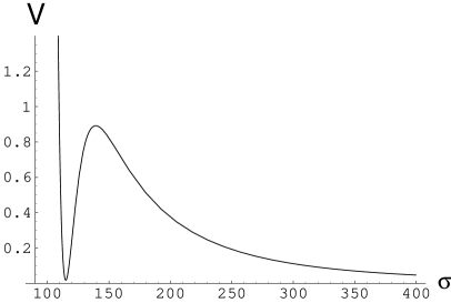
Figure 1: Potential (7.11) multiplied by $10^{15}$, taken from Ref.[184].

Actually, the value of $\sigma$ that minimizes the potential, $\sigma_{cr}$, is just slightly shifted from the one that gives the AdS minimum of the previous section, Eq.(7.9). The effect of the last term in (7.11), coming from the $\overline{\rm{D3}}$-branes, is therefore to lift the AdS minimum without changing too much the shape around the minimum.

The different versions of the uplifting mechanisms (Refs. [190, 191]) differ in the precise shape of the uplifting potential (7.10), but have the same overall behavior. The breaking of supersymmetry is spontaneous instead of explicit, as it is in KKLT. However, there are consistency requirements to combine D-term breaking with a non-perturbative superpotential (see Refs. [193, 194] for details).

Note that the de Sitter vacuum just obtained is metastable, as there is a runaway behavior to infinite volume. This is expected for many reasons. On one hand, it has become clear on entropy grounds that de Sitter space cannot be a stable state in any theory of quantum gravity [195]. On the other hand, the runaway behavior is a standard feature of all string theories [196]. Ref. [197] argues very generically that a positive vacuum energy in a space with extra dimensions implies an unstable universe toward decompactification. KKLT showed nevertheless that the lifetime of the dS vacuum is large in Planck times (it can be longer than the cosmological time scale $\sim 10^{10}$ years), and shorter than the recurrence time $t_{r}\sim e^{S}$, where $S$ is the dS entropy [195, 197]. Ref. [198] explored the possible decay channels of the KKLT de Sitter vacuum, finding, in agreement with KKLT, that even the fastest decays have decay times much greater than the age of our universe.

Let us note again that due to the critiques discussed in the previous section, KKLT is a toy model for getting de Sitter vacua in IIB compactifications. Differently from the case of AdS vacua, no explicit models with dS vacua were constructed so far (some partial constructions can be found for example in Ref.[199]). On top of the difficulties already discussed in stabilizing all moduli in a controlled way, there is an extra fine tuning needed in order to make the constant $D$ sufficiently small, and get at the same a long lived vacuum. There are however no fundamental reasons to doubt the existence of such explicit dS vacua.

Uplifts to de Sitter of IIA rigid Calabi-Yau orientifold flux vacua of the type discussed in section 6.4 were considered in Ref.[200] (see also Ref.[136] for moduli stabilization in IIA including corrections, and possible de Sitter vacua). De Sitter vacua are possible after taking into account non-perturbative corrections to the superpotential, and perturbative corrections to the Kähler potential. The latter give rise to a positive contribution analogous to the anti-D3-brane one of KKLT. Similarly, de Sitter vacua can be obtained from heterotic M-theory [201], using background fluxes and membrane instantons / gaugino condensation on the hidden boundary. In a very different spirit, Ref.[202] finds de Sitter vacua from flux compactifications on products of Riemann surfaces, while Ref.[203] finds dS vacua in supercritical string theories.

8 Distributions of flux vacua

It is somewhat clear from all the previous sections that the number of possible string/M theory vacua is very large. Despite the fact that as of today none of them fully reproduces the Standard Model data (hierarchy of masses, CKM matrix, etc, which in string theory vacua depend on moduli vevs), the hope is that adding sufficient number of ingredients to the soup, many of them could. This raises the “vacuum selection problem”: among the very large number (not clear whether it is even finite) of possible vacua, we have no idea which one is relevant, and how to find it. If there is no vacuum selection principle, i.e. no a priori condition that points toward the right candidate vacuum, the only way to find our vacuum seems to be by just enumerating all possible vacua, and testing each one against present observations. Since all possible vacua are too many (may be even infinite), Douglas and collaborators [204, 31, 32, 205] have advocated for a statistical study of the “landscape” of vacua, which could give some guidance principle for the search of the right vacuum. Let us review the basic ideas, and some of their results.

Given a set of effective $\mathcal{N}=1$ supergravity theories, i.e. a set of Kähler potentials $K_{i}$ and superpotentials $W_{i}$, with the same configuration space (the space in which the moduli take values), the first ingredient needed is the density $\rho$ of (susy or non susy) vacua. Integrating this density over a region $R$ in configuration space gives the number of vacua which stabilize moduli in that region, i.e.

$$\mathcal{N}_{\rm{vac},R}=\int_{R}d^{2n}z\,\rho(z)$$ (8.1)

where $z$ are the $n$ complex moduli fields. This density is given by

$$\rho(z)=\sum_{i}\delta^{n}(V^{\prime}_{i}(z))\,\,|{\rm det}\,V^{\prime\prime}_{i}(z)|$$ (8.2)

where $V_{i}$ is the $\mathcal{N}=1$ potential (5.26) for $K_{i}$, $W_{i}$. If the vacua are supersymmetric, this can be written in terms of the Kähler covariant derivatives as

$$\rho(z)_{\rm{susy}}=\sum_{i}\delta^{n}(DW_{i}(z))\,\delta^{n}(\overline{DW}_{i}(\bar{z}))\,\,|{\rm{det}}\,D^{2}W_{i}(z)|\ ,$$ (8.3)

where the Jacobian $D^{2}W$ is a $2n\times 2n$ matrix

$$D^{2}W=\left(\begin{array}[]{cc}D_{\bar{I}}D_{J}W(z)&\ D_{I}D_{J}W(z)\\ D_{\bar{I}}D_{\bar{J}}\bar{W}(\bar{z})&\ D_{I}D_{\bar{J}}\bar{W}(\bar{z})\end{array}\right)\ .$$ (8.4)

One can also find a density of supersymmetric vacua with a given cosmological constant, by multiplying (8.3) by $\delta(\Lambda-(-3e^{K_{i}}|W_{i}(z)|^{2}))$.

The ensemble of vacua that Douglas and collaborators consider are flux compactifications of F-theory on Calabi-Yau four-folds, or their IIB orientifolds limit. In the case of IIB vacua with 3-form fluxes on a Calabi-Yau orientifold, the Kähler potentials $K_{i}$ are all the same, Eq.(5.31) (or an equivalent expression with $\tau$ and $z$ together for the four-fold), while the superpotentials $W_{i}$, given in (5.48) are labeled by the $4(h^{2,1}_{-}+1)$ fluxes $(e_{K},m^{K},e_{K\,RR},m^{K}_{\rm RR})$. The tadpole cancellation condition (4.23) gives an upper bound for the number of units of flux (assuming we do not want to introduce $\overline{D3}$-branes), given by

$$N_{\rm{flux}}=e_{K}m^{K}_{{\rm RR}}-m^{K}e_{K\,{\rm RR}}=N\eta N\leq N_{*}\ ,\qquad N_{*}=\frac{\chi(X_{4})}{24}\ .$$ (8.5)

Let us illustrate this with the simplest example, considered in Ref. [31], of a rigid Calabi-Yau 3-fold ($h^{2,1}=0$). The only modulus of the theory appearing the flux superpotential is $\tau$, which is stabilized by the GVW superpotential (5.48)

$$W=(m^{0}F_{0}-e_{0}Z^{0})\tau+(-m^{0}_{{\rm RR}}F_{0}+e_{0\,{\rm RR}}Z^{0})\equiv C\tau+D\ .$$ (8.6)

The constants $Z^{0}=\int_{A}\Omega;\,F^{0}=\int_{B}\Omega$ are determined by the geometry of the Calabi-Yau.

Supersymmetric vacua obey

$$D_{\tau}W=\partial_{\tau}W-\frac{W}{\tau-\bar{\tau}}=-\frac{C\bar{\tau}+D}{\tau-\bar{\tau}}=0\ \ \ \Rightarrow\ \ \bar{\tau}=-\frac{D}{C}\ .$$ (8.7)

One can now scan all the possible values of $(e_{0},m^{0},e_{0,\,{\rm RR}},m^{0}_{\rm RR})$ satisfying the inequality (8.5), and get the corresponding value of the stabilized axion-dilaton. Taking $Z^{0}=1$, $\mathcal{F}_{0}=i$, $N_{*}=150$ and doing if necessary an $SL(2,{\mathbb{Z}})$ transformation to each resulting $\tau$ such that it is in the fundamental domain , Ref. [32] gets the distribution shown in Figure 2.

Figure 2: Values of $\tau$ for rigid CY flux vacua with $N_{*}=150$, $(Z^{0},\mathcal{F}_{0})=(1,i)$ , taken from Ref.[32].

The simplest example of flux vacua already gives an intricate distribution, from which it is hard to obtain any number (although Douglas and collaborators succeed in doing so), like for example the total number of vacua. However, Refs. [31, 32] show that for a sufficiently large region, the density of vacua per unit volume in moduli space can be well approximated by a constant, equal to $2\pi N_{*}^{2}$. This is a good approximation for disks of radii $R$ in moduli space if $R>\sqrt{1/N_{*}}$. The total number of vacua, Eq.(8.1), is therefore

$$\mathcal{N}_{\rm{susy}\,{vac}}(N_{\rm{flux}}<N_{*}) = \int_{\mathcal{M}_{\tau}}\rho(\tau)d^{2}\tau$$

$$\approx \int_{\mathcal{M}_{\tau}}2\pi N_{*}^{2}\frac{d^{2}\tau}{(2\text{Im}\tau)^{2}}=2\pi N_{*}^{2}\int_{\mathcal{M}_{\tau}}g_{\tau\bar{\tau}}\,d^{2}\tau=2\pi N_{*}^{2}\,\frac{\pi}{12}\ .$$

It is hard to believe looking at Figure 2 that the density is constant. One sees on one hand an accumulation of vacua close to the boundary, at $\tau$ =1, and with a sparser distribution for larger $\tau$. Additionally, there are voids around the points $\tau=ni$. The higher density for lower values of $\text{Im}\tau$ is just due to the modular invariant metric in moduli space, $d^{2}\tau/(2\text{Im}\tau)^{2}$. Regarding the holes, these are interpreted in Ref. [32] as consequences of the special conical shape of the region containing vacua. In any case, there is a very large degeneracy of vacua at the points $\tau=ni$ (there are for example 240 vacua at $\tau=2i$) which offsets the empty spaces, making the constant density approximation good for sufficiently large radii.

The rigid Calabi-Yau is a particularly simple case, we do not expect in general the density of vacua to be well approximated by a constant. But we do need a continuous approximation to the density in order to extract numbers out of Eq.(8.1). Such continuous approximation will replace the sum over the integer values of the fluxes by an integral, namely

$$\sum_{(e,m,e_{{\rm RR}},m_{{\rm RR}})\ \in\mathbb{Z}}\rightarrow\int\prod_{K=0}^{h^{2,1}_{-}}de_{K}\,dm^{K}\,de_{K,\,RR}\,dm^{K}_{{\rm RR}}\ .$$ (8.9)

(For a detailed discussion about the limitations of this approximation, see Ref. [31].) This integral should be cut off at a value given by the upper bound (8.5), i.e. it should be supplemented by a step function $\Theta(N_{\rm{flux}}-N_{*})$. Collecting all the pieces together, Ref [31] arrives at

$$\mathcal{N}_{\rm{susy}\,{vac}} = \sum_{\rm{susy}\ {vac}}\Theta(N_{\rm{flux}}-N_{*})$$

$$\approx \frac{1}{2\pi i}\int_{C}\frac{d\alpha}{\alpha}e^{\alpha N_{*}}\int d^{2p}z\int d^{4p}Ne^{-\frac{\alpha}{2}N\eta N}\delta^{p}(DW(z))\,|{\rm det}\,D^{2}W(z)|$$

where we have used the Laplace transform in $\alpha$ of the step function, and defined $p=h^{2,1}_{-}+1$.

Skipping the details of the calculation, which the reader is welcome to follow from Refs. [31, 32], we quote the result. A good approximation for the number of type IIB O3/O7 supersymmetric vacua inside a region $R$ in moduli space is given by

$$\mathcal{N}_{\rm{susy}\,{vac}}\,(N_{\rm{flux}}\leq N_{*})\approx\frac{(2\pi N_{*})^{2p}}{\pi^{p}(2p)!}\int_{R}{\rm{det}}({\mathbb{R}}+J\,{\mathbb{I}})\ ,\quad p=h^{2,1}_{-}+1\ .$$ (8.11)

In this equation, ${\mathbb{R}}$ is the curvature two-form in the $2p$ dimensional moduli space expressed as a $p\times p$ matrix, namely $({\mathbb{R}})_{ab}=R_{k\bar{l}ab}\,dz^{k}\wedge d\bar{z}^{l}$ ($a,b$ are orthonormal frame indices, and $k,l$ tangent space indices in moduli space); $J$ is the Kähler two-form $J_{k\bar{l}}\,dz^{k}\wedge d\bar{z}^{l}$ and ${\mathbb{I}}$ is the $p\times p$ identity matrix $\delta_{ab}$.

We see that the constant density for the case of a rigid Calabi-Yau is replaced by a “topological” density

$$\rho(z)_{\rm susy}=\frac{(2\pi N_{*})^{2p}}{\pi^{p}(2p)!}\rm{det}({\mathbb{R}}+J\,{\mathbb{I}})\ .$$ (8.12)

This is actually an “index” density: it counts the number of vacua with signs, i.e. dropping the absolute value of the determinant in Eq.(8.3). It therefore gives a lower bound to the density of vacua. Ref. [31] argues that (8.12) is a good lower bound for the number of flux vacua for $N_{*}\gg 2p\gg 1$, and that the total number of vacua is probably (8.11) multiplied by $c^{2p}$, with some $c\sim 1$.

The index density (8.12) agrees with the constant $2\pi N_{*}^{2}$ per unit volume in $\mathcal{M}_{\tau}$ for the rigid ($p=1$) case. This means that the vacuum expectation values of the dilaton, or the string coupling constant, is in good approximation uniformly distributed. Integrating the density over a fundamental domain in moduli space, gives the number of supersymmetric flux vacua for a given Calabi-Yau.

Given the formula for the total number of vacua, the first question to ask is whether this number is finite. It has been conjectured that the volumes of these moduli spaces are finite [207], which restricts the question of finiteness to possible divergences coming from the curvature. A typical case in which the curvature diverges is the neighborhood of a conifold point. However, Ref. [31] shows that for the complex structure moduli space of the mirror quintic (expecting conifold points on other CY’s to have the same behavior), in spite of $R$ being singular, the integral is finite. With more moduli there might be more complicated degenerations, but there is reasonable hope that the number $\mathcal{N}_{\rm{susy}\,{vac}}(N_{\rm{flux}}<N_{*})$ is finite .

Let us now illustrate with the next to simplest example: a moduli space of complex dimension $p=2$, i.e. consisting of the dilaton-axion plus one complex structure modulus, $\mathcal{M}=\mathcal{M}_{\tau}\times\mathcal{M}_{Y}$. The metric ${\mathbb{R}}+J\,{\mathbb{I}}$ is

$${\mathbb{R}}+J\,{\mathbb{I}}=\left(\begin{array}[]{cc}R_{0}+J_{0}+J_{1}&0\\ 0&R_{1}+J_{0}+J_{1}\end{array}\right)$$ (8.13)

where we have defined

$$\begin{array}[]{cc}R_{0}\equiv R_{\tau\bar{\tau}}\,d\tau\wedge d\bar{\tau}\ \ ,&J_{0}\equiv J_{\tau\bar{\tau}}\,d\tau\wedge d\bar{\tau}\\ R_{1}\equiv R_{z\bar{z}}\,dz\wedge d\bar{z}\ \ ,&J_{1}\equiv J_{z\bar{z}}\,dz\wedge d\bar{z}\end{array}$$ (8.14)

It is easy to check that for the metric on $\mathcal{M}_{\tau}$, given by the Kähler potential $K=-\ln\left[-i(\tau-\bar{\tau})\right]$, $R_{0}=-2J_{0}$. The determinant of (8.14) is therefore given by

$$\rm{det}({\mathbb{R}}+J\,{\mathbb{I}})=(-J_{0}+J_{1})\wedge(R_{1}+J_{0}+J_{1})=-J_{0}\wedge R_{1}\ .$$ (8.15)

Inserting this in (8.11), and using $\int_{\mathcal{M}_{\tau}}J_{0}=\tfrac{\pi}{12}$ (cf. Eq.(8)), gives

$$\mathcal{N}_{\rm{susy}\,{vac}}\,(N_{\rm{flux}}\leq N_{*})\approx-\frac{(2\pi N_{*})^{4}}{\pi^{2}4!}\frac{\pi}{12}\int_{\mathcal{M}_{Y}}R_{z\bar{z}}\,dz\wedge d\bar{z}=-\frac{(2\pi N_{*})^{4}}{4!\,6}\chi(\mathcal{M}_{Y})$$ (8.16)

In this next to simplest example, the number of vacua is therefore just proportional to the Euler characteristic of the complex structure modulus space (and to the usual power $N_{*}^{2p}=N_{*}^{4}$).

Let us apply this to a manifold $Y$ with a conifold degeneration [32]. As in the case of the deformed conifold of section 6.1 (see below Eq.(6.3)), the periods are $Z(z)=z$, $\mathcal{F}(z)=\frac{z}{2\pi i}+$ analytic terms. Inserting this in the Kähler potential (5.31), we get $K\approx-\ln[\tfrac{1}{2\pi}|z|^{2}\ln|z|^{2}]$. This gives the following metric near $z=0$

$$g_{z\bar{z}}\approx c\,\,\ln\frac{1}{|z|^{2}}$$ (8.17)

where $c=e^{K_{0}}/2\pi$, with $K_{0}$ the Kähler potential at $z=0$. The curvature is therefore

$$R_{z\bar{z}}\approx-\frac{1}{|z|^{2}\,\ln|z|^{2}}\ .$$ (8.18)

This implies that the density (8.12) diverges at the conifold point, $z=0$. The integral over a finite domain $|z|<R$ is nevertheless finite, namely

$$\mathcal{N}_{\rm{susy}\,{vac}}\,(N_{\rm{flux}}\leq N_{*})\approx-\frac{(2\pi N_{*})^{4}}{\pi^{2}4!}\frac{\pi}{12}\int_{|z|<R}R_{z\bar{z}}\,dz\wedge d\bar{z}\approx\frac{(\pi N_{*})^{4}}{18\,\ln\frac{1}{R^{2}}}$$ (8.19)

The logarithmic dependence implies that a very large number of vacua are extremely close to the conifold point. For example, for $N_{*}=100$, there are about one million vacua with $|z|<10^{-100}$. This is a good feature from the phenomenological point of view, since small vev’s for the complex structure modulus generate large hierarchies [22], as in Eq.(6.6).

Very similarly to the example with $p=2$, we can compute the number of vacua for tori with diagonal period matrix, i.e. take $\kappa^{ij}$ in Eq. (6.8) to be $\kappa^{ij}=\kappa^{i}\,\delta^{ij}$. There are 4 complex moduli: 3 complex structure $\kappa^{i}$ and the dilaton-axion. Given the holomorphic 3-form in Eq. (6.9), the Kähler potential, Eq.(5.31), is

$$K = -\ln[-i(\tau-\bar{\tau})]-\ln\Big{[}-i\int\Omega(\kappa)\wedge\overline{\Omega}(\bar{\kappa})\Big{]}$$ (8.20)

$$= -\ln[-i(\tau-\bar{\tau})]-\ln[\rm{det}\,\text{Im}\kappa]=-\sum_{p=0}^{3}{\rm ln}[-i(w^{p}-\bar{w}^{p})]$$

where ${\rm w^{p}}=(\tau,\kappa^{i})$. There are therefore four copies of the moduli space $\mathcal{M}_{\tau}$. When building the 4 x 4 matrix (8.15), we can use $R_{i}=-2\,J_{i}$, (see below Eq.(8.14)). We therefore have

$$\rm{det}({\mathbb{R}}+J\,{\mathbb{I}})=8\,J_{0}\wedge J_{1}\wedge J_{2}\wedge J_{3}\ .$$ (8.21)

This is a combinatoric factor times the volume form of the total moduli space. The fundamental region has a permutation symmetry, i.e. is preserved by $SL(2,{\mathbb{Z}})^{p}\times S_{p}$, so its volume is

$$V_{p}=\frac{1}{p!}\left(\frac{\pi}{12}\right)^{p}$$ (8.22)

The number of vacua is therefore

$$\mathcal{N}_{\rm{susy}\,{vac}}(N_{\rm{flux}}<N_{*})=8\frac{(2\pi N_{*})^{8}}{\pi^{4}8!}\frac{1}{4!}\left(\frac{\pi}{12}\right)^{4}=\frac{1}{3}\frac{(2\pi N_{*})^{8}}{(12)^{4}\,8!}\ .$$ (8.23)

For $N_{*}=16$, which is the value for a $T^{6}$ with 64 O3-planes, we have about four million supersymmetric vacua.

Typical Calabi-Yau’s have many more complex structure moduli, leading to many more possible vacua. For example, Ref. [79] finds several supersymmetric flux vacua for the Calabi-Yau 3-fold hypersurface in $WP_{1,1,1,1,4}$. The 3-fold has $h^{2,1}=149$, and its orientifold descends from the F-theory Calabi-Yau 4-fold in $WP_{1,1,1,1,8,12}$, which has $\chi/24=972$. We can roughly estimate the number of vacua to be of the order $10^{230}$.

After looking at these huge numbers of vacua, we can convince ourselves that searching for vacua one by one until we reach the right one does not seem to be a clever idea. It is true nevertheless that we are not imposing any observational constraint on these vacua (like cosmological constant, spectrum…). Imposing such constraints the numbers should reduce. Clearly, none of these vacua has a positive cosmological constant, but we could nevertheless demand that $|W|$ is smaller than a given value such that the KKLT (or its variations thereof) uplifting mechanism could work. Let us see then how the constraint $|W|^{2}\leq\lambda_{*}$ reduces the numbers.

$|W|^{2}<\lambda$ is enforced by inserting a delta $\delta(|W|^{2}-\lambda)$ in (8) and integrate over $\lambda$ up to $\lambda_{*}$. This seems like an easy task to do. However, there is no nice topological formula such as (8.11) for the index density when one includes this restriction. Instead, Eq. (8.12) becomes

$$\rho(z,\lambda)_{\rm susy}=\Theta(N_{*}-\lambda)\frac{(2p)!\,(N_{*}-\lambda)^{2p-1}}{(\pi N_{*})^{p}}\sum_{k=0}^{p}\frac{c_{k}(z)}{(2p-1-k)!}\left(\frac{\lambda}{N_{*}-\lambda}\right)^{k}\ ,$$ (8.24)

where $c_{k}(z)$ are homogeneous polynomial functions. We see that the cosmological constant is smaller than $N_{*}$, and the density for $\lambda\sim N_{*}$ is suppressed by a factor $(N_{*}-\lambda)^{p-1}$. Because of this suppression, for large $p$ we expect the distribution to be peaked at small $\lambda$. Integrating (8.24) up to a small value $\lambda_{*}$, we see that the fraction of vacua with $|\lambda|\leq\lambda_{*}$ behaves like $\lambda_{*}/N_{*}$ (in units of $1/(2\pi\sqrt{\alpha^{\prime}})^{4}$). This implies that the smallest cosmological constant is of order $\alpha^{\prime 2}/\mathcal{N}_{\rm{vac}}$. Vacuum multiplicity would therefore help in solving the cosmological constant problem.

Another important feature about the distribution of flux vacua, is that it is suppressed in the large complex structure region. With one complex structure modulus, and in the large complex structure limit, the Kähler potential $\int\Omega\wedge\bar{\Omega}$ has an expansion of the form $-{\rm ln}[i(z-\bar{z})^{3}]$, resembling the expression for the Kähler moduli $t$, Eq.(5.9). We saw that for this Kähler potential $R_{z\bar{z}}\propto g_{z\bar{z}}$, and therefore the density of vacua per unit volume in moduli space is constant. The index density (8.12) goes therefore like $d\rho(z)\sim g_{z\bar{z}}d^{2}z\sim\frac{d^{2}z}{(z-\bar{z})^{2}}$. This density behaves like that of Figure 2. We see therefore that the large complex structure limit region is strongly suppressed. In the mirror IIA picture, $\text{Im}z$ is mapped to $\text{Im}t\sim V^{1/3}$ (where $V$ is the volume). This gives a number of vacua that falls off with volume as $V^{-1/3}$. For $n$ complex structure moduli (or many Kähler moduli in the mirror picture), there is a large volume falloff as $V^{-n/3}$.

Ref. [206] studies the density of non supersymmetric (F-breaking) flux vacua, given by (8.2). We will not review the details here, but just quote one of their main results. The number of metastable vacua with F-term supersymmetry breaking scale $M_{\rm{s\not usy}}<M_{*}$ inside a region $R$ is related to that of supersymmetric vacua by

$$N_{\rm{s\not usy},\rm{R}}(M_{\rm{s\not usy}}<M_{*})=M^{2}_{*}N_{\rm{susy},\rm{R}}\ .$$ (8.25)

If one imposes additionally that the cosmological constant be smaller than a given small value $\lambda_{*}$, this ratio is

$$N_{\rm{s\not usy},\rm{R}}(M_{\rm{s\not usy}}<M_{*},\lambda<\lambda_{*})=M^{12}_{*}\lambda_{*}N_{\rm{susy},\rm{R}}\ ,\qquad\lambda_{*}<|F|,|W|$$ (8.26)

Low scale supersymmetry breaking is therefore disfavored

As mentioned, there is no constraint imposed regarding the matter content of these flux vacua. In that respect, Ref. [204] gives a first estimate of the fraction of vacua that have Standard Model spectrum (see Ref. [209] for some explicit D-brane models statistics). The case analyzed corresponds to SM matter arising from D6-branes in IIA wrapping 3 cycles of Calabi-Yau’s. The fraction of vacua that have a $U(3)\times U(2)\times U(1)^{2}$ gauge group is roughly $10^{-6}$. While the estimates of Ref [204] are very crude, the conjecture is that ignoring values for the couplings, the fraction of models which realize the standard model spectrum is closer to ${\mathcal{O}}(10^{-10})$ than to ${\mathcal{O}}(10^{-100})$.

Let us summarize the prominent features of the distribution of supersymmetric vacua.

$\bullet$ The density of dilaton-axion vev’s is constant per unit volume in moduli space.
$\bullet$ Vacua accumulate near conifold points.
$\bullet$ The distribution of values of cosmological constant is uniform near zero.
$\bullet$ The distribution has a falloff at large complex structure, or in the mirror manifold, at large volume as $\mathcal{N}\sim V^{-\frac{p-1}{3}}$.
$\bullet$ High scale supersymmetry breaking is favored.

Statistics of M-theory vacua have been put forward in the same spirit in Ref. [218], while some “rudimentary statistics” in a simple IIA toy model are performed in Ref. [24].

Although still a bit premature to drive final conclusions from the distributions of flux vacua, Douglas and collaborators have made a big step toward developing a statistical approach to flux compactifications. The first conclusion seems to be that even after imposing metastability, acceptable supersymmetry breaking and a Standard Model spectrum, the number of vacua seems to be very large, probably too large to be explored one by one, making it useful to study their distribution statistically. This distribution shows many simple properties, such as large volume and low supersymmetry breaking suppression.

To finish this section, let us point out that the distribution of supersymmetric IIB flux vacua (8.12), in particular its behavior on the moduli space geometry as $\rm{det}({\mathbb{R}}+J\,{\mathbb{I}})$; its growth with $N_{*}$ as $N_{*}^{2p}$ as well as its conifold attractor point have been tested using Monte Carlo experiments in Refs. [80, 162] (see also Ref. [210]). Ref. [80] studies the mirror of an orientifold of the CY hypersurface in $P_{1,1,1,1,4}$, which has $p=2$ (one complex structure modulus) and $N_{*}=972$. Refs. [162, 211] analyze the mirror of the CY hypersurface $P_{1,1,2,2,6}$, which has two complex structure moduli.

9 Summary and future prospects

It is clear that flux compactifications in string theory has been an extremely active and fruitful area of research, particularly in the past five years. The main reason for this flurry of activity is that fluxes are the only known perturbative mechanism that stabilizes moduli. In many setups, most notably in all IIB compactifications on Calabi-Yau’s or tori, closed string fluxes are not enough to stabilize all moduli. Therefore, other perturbative and non perturbative mechanisms, some of which we do not have enough theoretical control yet, have to be invoked. However, fluxes were shown very recently to be enough to stabilize all moduli in IIA compactifications on rigid tori and on twisted tori, and similarly all moduli can in principle be stabilized in IIB by considering additionally open string fluxes. While stabilizing moduli, fluxes break supersymmetry partially or completely in a stable way, and generate warp factors, giving stringy mechanisms of realizing large hierarchies. Fluxes have also served as an ingredient in the construction of semi-realistic four-dimensional vacua with Standard Model spectra.

In all these models, the back-reaction of the geometry is basically neglected. The back-reacted internal geometry involves, in all flux backgrounds, manifolds with torsion. In spite of the recent progress in understanding their mathematical properties, and therefore the four-dimensional resulting physics, many of the very basic questions such as what are their moduli spaces are still widely unanswered. However, conformally-Ricci-flat manifolds (like conformal Calabi-Yau’s or tori) allow for non trivial fluxes, and give us a way of studying the effective theories with the available mathematical tools (in most cases neglecting, however, the conformal factor). In the absence of fluxes, these leave $\mathcal{N}=8,4,2$ unbroken supersymmetries in four-dimensions, while turning on fluxes breaks these to $\mathcal{N}=4,3,2,1,0$. Most of the analysis of moduli stabilization has been carried out in this class of compactifications.

There are explicit constructions of flux compactifications with all moduli stabilized. In type IIB, these use non-perturbative effects in sufficiently sophisticated internal manifolds that have the right cycles to support the corrections, and are non-supersymmetric. In type IIA, the explicit constructions involve rigid orientifolds of tori orbifolds, where all moduli can be stabilized in $\mathcal{N}=1$ supersymmetric AdS vacua, or orientifolds of twisted tori, where there are additional Minkowski vacua with all moduli fixed except for some axions. Besides, metastable de Sitter vacua in IIB can also be attained using (supersymmetry breaking) fluxes and non-perturbative effects.

Flux compactifications have many additional interconnected aspects / applications that we have not discussed in depth in this review, or have not discussed at all. First of all, there is much more to report about the gauged supergravity interpretation of certain flux compactifications [212, 23] (for a short review, see [213]). Besides, we have not discussed the relation between flux compactifications on twisted tori and Scherk-Schwarz compactifications [214] (see Refs.[157, 215]). Neither have we discussed non-geometric backgrounds [95], which are sometimes dual to geometric flux vacua. Another undiscussed area is that of topological strings [221], in particular the attractor mechanism [222] and the Ooguri-Strominger-Vafa conjecture [223].

On a more phenomenological level, fluxes generate supersymmetric and soft supersymmetry breaking terms on D-branes [144, 216, 177, 217], which can stabilize open string moduli [35, 36, 34]. (In the presence of fluxes, the supersymmetric cycles wrapped by D-branes are also modified, in order to minimize the action [43, 220].) Soft-supersymmetry breaking effects and moduli stabilization in KKLT type scenarios has been discussed extensively (see for example [164, 185, 219]). Some other phenomenological applications that we have not discussed much are, for example, the landscape of supersymmetry breaking vacua and supersymmetry breaking scales [224] (see Ref. [32] for a statistical analysis); and models of inflation embedded in flux compactification scenarios, started most notably by Ref. [225].

Some non-compact flux backgrounds play a very important role in AdS/CFT, as they can realize string duals of confining gauge theories (see [226] for a review). Latest developments along these lines involve the recent explicit construction of conical Calabi-Yau metrics over the Sasaki-Einstein manifolds $Y^{p,q}$ [227] and $L^{p,q,r}$ [228]. Their dual conformal field theories were found in Ref. [229]. However, there are no complex structure deformations on these manifolds, and opposite to the case in Klebanov-Strassler’s solution, adding 3-form fluxes does not seem to lead to regular supersymmetric backgrounds [230].

By turning on appropriate fluxes (which requires sometimes some fine tuning), moduli are stabilized in the regime where we can trust the effective field theory approximation. This needs a (string frame) volume or radius much bigger than the KK and string scales, ans a small coupling constant (or more the more restrictive condition $g_{s}N_{\rm{flux}}\ll 1$). Nevertheless, specific (small) numbers like the cosmological constant in non-supersymmetric solutions are subject to corrections which can be of the same order of magnitude as the leading order value, and cannot therefore be fully trusted. Corrections are however expected to be small if the vacuum energy is itself much smaller than the string scale and KK scale to the fourth power. In any case, leaving aside the phenomenology of scales, it is conceivable that in some of these backgrounds a subsector of the theory develops an instability, and we are dropping in the effective Lagrangian a KK or stringy mode which is tachyonic. Backgrounds with NS fluxes can be studied in the other extreme regime, where the internal space is very small, but world-sheet techniques are powerful enough, like in orientifolds of Gepner models [231] (see Ref [232] for a search of vacua with Standard Model spectra in Gepner models). The analysis of backgrounds with RR flux using world-sheet techniques is on the contrary still far from being available, although a lot of progress in this direction is expected (or hoped) to happen: a new formalism for a covariant quantization of the superstring which allows to study backgrounds with RR flux was introduced a few years ago [233]. As as of today, however, loop amplitudes have only been obtained in highly symmetric backgrounds like $AdS_{5}\times S^{5}$ or the pp-wave.

A fair concluding remark would be that we have made huge progress in the past years, but there is still a lot of work ahead of us to see whether the available models of flux compactifications are as copious and rich as they appear today, and whether our four-dimensional world is one of them.

Appendix A Conventions

$\bullet$ We use the following index notation

- $\mu,\nu,...=0,...,3$ label external coordinates.

- $m,n,...=1,...,6$ label real internal coordinates.

- $i,j=1,2,3$, $\bar{\imath},\bar{\jmath}=1,2,3$ label internal complex coordinates.

- $M,N,...=0,...,9$ label all coordinates.

$\bullet$ We switch back and forth between Einstein frame and string frame. Section 3 is entirely in string frame. Most of section 4 is also in string frame, except Eqs. (4.14), (4.34) and (4.35) (all taken from Ref.[22]), which are in Einstein frame. Sections 5 and on are in Einstein frame.

$\bullet$ The different RR field strengths used (standard, modified, internal, external) are

-$\hat{F}_{n}=dC_{n-1}$ is the standard RR field strength, and $F^{(10)}$ is the modified one. Explicitly,

$$F^{(10)}=dC-H\wedge C+m\,e^{B}=\hat{F}-H\wedge C$$ (A.1)

-The modified flux is split into internal and external components according to

$$F^{(10)}_{n}=F_{n}+\rm{Vol}_{4}\wedge\tilde{F}_{n-4}\ .$$ (A.2)

Hodge dualities among the components given in Eqs (2.3, 3.5).

$\bullet$ A $\star$ symbol means 10-dimensional Hodge duality, while we use $*$ for internal (6D) Hodge duality.

$\bullet$ Whenever factors of $\alpha^{\prime}$ are not written explicitly, we are taking $(2\pi)^{2}\alpha^{\prime}=1$.

$\bullet$ We use the standard decomposition of the ten-dimensional gamma matrices $\Gamma^{M}=(\Gamma^{\mu},\Gamma^{m})$ as

$$\Gamma^{\mu}=\gamma^{\mu}\otimes 1,\quad\mu=0,1,2,3\ ,\qquad\Gamma^{m}=\gamma_{5}\otimes\gamma^{m}\ ,\quad m=1,\ldots,6\ ,$$ (A.3)

and

$$\gamma_{5}=\tfrac{i}{4!}\epsilon_{\mu\nu\lambda\rho}\gamma^{\mu\nu\lambda\rho}\,,\qquad\gamma_{7}=-\tfrac{i}{6!}\epsilon_{mnpqrs}\gamma^{mnpqrs}\,,\qquad\gamma_{11}=\gamma_{5}\,\gamma_{7}$$ (A.4)

The $\gamma^{m}$ are Hermitean, as are the $\gamma^{\mu}$, except $\gamma^{0}$ which is antihermitean.

$\bullet$ A slash is defined in the following way

$$/\!\!\!\!{F_{n}}=\frac{1}{n!}F_{P_{1}...P_{N}}\Gamma^{P_{1}...P_{N}}\ ,\qquad\Gamma^{P_{1}...P_{N}}=\Gamma^{[P_{1}}...\Gamma^{P_{N}]}\ .$$ (A.5)

For the SU(3) structure, the norm of the normalized spinor is

$$\eta^{\dagger}\eta=\eta_{+}^{\dagger}\eta_{+}+\eta_{-}^{\dagger}\eta_{-}=1\ .$$ (A.6)

$\bullet$ The fundamental 2-form and holomorphic 3-form constructed from this spinor as in (3.14) obey

$$J\wedge J\wedge J=\frac{3i}{4}\,\Omega\wedge\bar{\Omega}\ .$$ (A.7)

$\bullet$ The decomposition of a 2-,3-,4-,5- and 6-form in SU(3) representations used in section 3.3 is

$$F_{1} = F_{1}^{(3)}+F_{3}^{(\bar{3})}$$

$$F_{2} = \frac{1}{3}F_{2}^{(1)}\,J+\text{Re}(F_{2}^{(3)}\llcorner\overline{\Omega})+F_{2}^{(8)}\,,$$

$$F_{3} = -\frac{3}{2}\,{\rm Im}(F_{3}^{(1)}\bar{\Omega})+(F_{3}^{(3)}+F_{3}^{(\bar{3})})\wedge J+F_{3}^{(6)}+F_{3}^{(\bar{6})}\,,$$

$$F_{4} = \frac{1}{6}F_{4}^{(1)}J\wedge J+Re(F_{4}^{(3)}\wedge\overline{\Omega})+F_{4}^{(8)}\,,$$

$$F_{5} = (F_{5}^{(3)}+F_{5}^{(\bar{3})})\wedge J\wedge J\,,$$

$$F_{6} = \frac{1}{6}F_{6}^{(1)}\,J\wedge J\wedge J\,,$$ (A.8)

The inverse relations are

$$(F_{1}^{(3)})_{i} = F_{i}$$

$$F_{2}^{(1)} = \frac{1}{2}F_{mn}J^{mn}=F_{i\bar{\jmath}}J^{i\bar{\jmath}}$$

$$F_{3}^{(1)} = -\frac{i}{36}F^{ijk}\Omega_{ijk}\,,\qquad\quad(F_{3}^{(3)})_{i}=\frac{1}{4}F_{imn}J^{mn}\,,\qquad(F_{3}^{(6)})_{ij}=F^{kl}\,_{(i}\Omega_{j)kl}$$

$$F_{4}^{(1)} = \frac{1}{8}F^{mnpq}J_{mn}J_{pq}\,,\qquad(F_{4}^{(3)})_{k}=\frac{1}{24}F_{k}\,^{ijl}\Omega_{ijl}\,$$

$$(F_{5}^{(3)})_{i} = \frac{1}{16}F_{i}^{mnpq}J_{mn}J_{pq}\,$$

$$F_{6}^{(1)} = \frac{1}{48}F^{mnpqrs}J_{mn}J_{np}J_{qr}$$ (A.9)

These can be used to obtain the torsion classes in (3.2) in terms of $dJ,d\Omega,J$ and $\Omega$.

References

References

- [1]
- [2] Candelas, Horowitz, Strominger, Witten P. Candelas, G. T. Horowitz, A. Strominger and E. Witten, “Vacuum Configurations For Superstrings,” Nucl. Phys. B 258, 46 (1985).
-
[3]
C. M. Hull,
“Superstring Compactifications With Torsion And Space-Time
Supersymmetry,”
Print-86-0251 (CAMBRIDGE)
A. Strominger, “Superstrings With Torsion,” Nucl. Phys. B 274 (1986) 253. -
[4]
Some of the first constructions are
E. Witten,
“New Issues In Manifolds Of SU(3) Holonomy,”
Nucl. Phys. B 268, 79 (1986).
B. R. Greene, K. H. Kirklin, P. J. Miron and G. G. Ross, “A Three Generation Superstring Model. 2. Symmetry Breaking And The Low-Energy Theory,” Nucl. Phys. B 292, 606 (1987).
I. Antoniadis, J. R. Ellis, J. S. Hagelin and D. V. Nanopoulos, “An Improved SU(5) X U(1) Model From Four-Dimensional String,” Phys. Lett. B 208, 209 (1988) [Addendum-ibid. B 213, 562 (1988)].
For the most recent heterotic string Satandard Model construction, see V. Braun, Y. H. He, B. A. Ovrut and T. Pantev, “A heterotic standard model,” Phys. Lett. B 618, 252 (2005) [arXiv:hep-th/0501070]. -
[5]
J. P. Derendinger, L. E. Ibanez and H. P. Nilles,
“On The Low-Energy D = 4, N=1 Supergravity Theory Extracted From The D = 10,
N=1 Superstring,”
Phys. Lett. B 155, 65 (1985).
M. Dine, R. Rohm, N. Seiberg and E. Witten, “Gluino Condensation In Superstring Models,” Phys. Lett. B 156, 55 (1985).
- [6] For a review, see for example F. Quevedo, “Lectures on superstring phenomenology,” arXiv:hep-th/9603074.
- [7] C. Bachas, “A Way to break supersymmetry,” arXiv:hep-th/9503030.
- [8] J. Polchinski, “Dirichlet-Branes and Ramond-Ramond Charges,” Phys. Rev. Lett. 75, 4724 (1995) [arXiv:hep-th/9510017].
-
[9]
For a review, see for example
A. M. Uranga,
“Chiral four-dimensional string compactifications with intersecting
D-branes,”
Class. Quant. Grav. 20, S373 (2003)
[arXiv:hep-th/0301032].
E. Kiritsis, “D-branes in standard model building, gravity and cosmology,” Fortsch. Phys. 52, 200 (2004) [arXiv:hep-th/0310001].
D. Lust, “Intersecting brane worlds: A path to the standard model?,” Class. Quant. Grav. 21, S1399 (2004) [arXiv:hep-th/0401156]. - [10] J. Polchinski and A. Strominger, “New Vacua for Type II String Theory,” Phys. Lett. B 388 (1996) 736 [arXiv:hep-th/9510227].
- [11] J. Michelson, “Compactifications of type IIB strings to four dimensions with non-trivial classical potential,” Nucl. Phys. B 495, 127 (1997) [arXiv:hep-th/9610151].
- [12] T. R. Taylor and C. Vafa, “RR flux on Calabi-Yau and partial supersymmetry breaking,” Phys. Lett. B 474 (2000) 130 [arXiv:hep-th/9912152].
- [13] M. Graña and J. Polchinski, “Supersymmetric three-form flux perturbations on AdS(5),” Phys. Rev. D 63, 026001 (2001) [arXiv:hep-th/0009211]; “Gauge / gravity duals with holomorphic dilaton,” Phys. Rev. D 65, 126005 (2002) [arXiv:hep-th/0106014].
- [14] S. S. Gubser, “Supersymmetry and F-theory realization of the deformed conifold with three-form flux,” arXiv:hep-th/0010010.
- [15] A. R. Frey and J. Polchinski, “N = 3 warped compactifications,” Phys. Rev. D 65, 126009 (2002) [arXiv:hep-th/0201029].
- [16] S. Kachru, X. Liu, M. B. Schulz and S. P. Trivedi, “Supersymmetry changing bubbles in string theory,” JHEP 0305, 014 (2003) [arXiv:hep-th/0205108].
- [17] J. M. Maldacena, “The large N limit of superconformal field theories and supergravity,” Adv. Theor. Math. Phys. 2, 231 (1998) [Int. J. Theor. Phys. 38, 1113 (1999)] [arXiv:hep-th/9711200].
- [18] J. Polchinski and M. J. Strassler, “The string dual of a confining four-dimensional gauge theory,” arXiv:hep-th/0003136.
- [19] I. R. Klebanov and M. J. Strassler, “Supergravity and a confining gauge theory: Duality cascades and chiSB-resolution of naked singularities,” JHEP 0008, 052 (2000) [arXiv:hep-th/0007191].
- [20] J. M. Maldacena and C. Nuñez, “Towards the large N limit of pure N = 1 super Yang Mills,” Phys. Rev. Lett. 86, 588 (2001) [arXiv:hep-th/0008001].
- [21] K. Dasgupta, G. Rajesh and S. Sethi, “M theory, orientifolds and G-flux,” JHEP 9908, 023 (1999) [arXiv:hep-th/9908088].
- [22] S. B. Giddings, S. Kachru and J. Polchinski, “Hierarchies from fluxes in string compactifications,” Phys. Rev. D 66, 106006 (2002) [arXiv:hep-th/0105097].
-
[23]
J. P. Derendinger, C. Kounnas, P. M. Petropoulos and F. Zwirner,
“Superpotentials in IIA compactifications with general fluxes,”
Nucl. Phys. B 715, 211 (2005)
[arXiv:hep-th/0411276].
G. Villadoro and F. Zwirner, “N = 1 effective potential from dual type-IIA D6/O6 orientifolds with general fluxes,” JHEP 0506, 047 (2005) [arXiv:hep-th/0503169]. - [24] O. DeWolfe, A. Giryavets, S. Kachru and W. Taylor, “Type IIA moduli stabilization,” arXiv:hep-th/0505160.
- [25] P. G. Camara, A. Font and L. E. Ibanez, “Fluxes, moduli fixing and MSSM-like vacua in a simple IIA orientifold,” arXiv:hep-th/0506066.
-
[26]
L. Randall and R. Sundrum,
“A large mass hierarchy from a small extra dimension,”
Phys. Rev. Lett. 83, 3370 (1999)
[arXiv:hep-ph/9905221].
L. Randall and R. Sundrum, “An alternative to compactification,” Phys. Rev. Lett. 83, 4690 (1999) [arXiv:hep-th/9906064]. - [27] H. L. Verlinde, “Holography and compactification,” Nucl. Phys. B 580, 264 (2000) [arXiv:hep-th/9906182].
- [28] J. M. Maldacena and C. Nuñez, “Supergravity description of field theories on curved manifolds and a no go theorem,” Int. J. Mod. Phys. A 16, 822 (2001) [arXiv:hep-th/0007018].
- [29] R. Bousso and J. Polchinski, “Quantization of four-form fluxes and dynamical neutralization of the cosmological constant,” JHEP 0006, 006 (2000) [arXiv:hep-th/0004134].
- [30] L. Susskind, “The anthropic landscape of string theory,” arXiv:hep-th/0302219.
- [31] S. Ashok and M. R. Douglas, “Counting flux vacua,” JHEP 0401, 060 (2004) [arXiv:hep-th/0307049].
-
[32]
F. Denef and M. R. Douglas,
“Distributions of flux vacua,”
JHEP 0405, 072 (2004)
[arXiv:hep-th/0404116].
F. Denef and M. R. Douglas, “Distributions of nonsupersymmetric flux vacua,” JHEP 0503, 061 (2005) [arXiv:hep-th/0411183]. - [33] B. S. Acharya, F. Denef and R. Valandro, “Statistics of M theory vacua,” JHEP 0506, 056 (2005) [arXiv:hep-th/0502060].
- [34] D. Lust, P. Mayr, S. Reffert and S. Stieberger, “F-theory flux, destabilization of orientifolds and soft terms on D7-branes,” arXiv:hep-th/0501139.
- [35] R. Blumenhagen, M. Cvetic, F. Marchesano and G. Shiu, “Chiral D-brane models with frozen open string moduli,” JHEP 0503, 050 (2005) [arXiv:hep-th/0502095].
-
[36]
I. Antoniadis, A. Kumar and T. Maillard,
“Moduli stabilization with open and closed string fluxes,”
arXiv:hep-th/0505260.
J. Gomis, F. Marchesano and D. Mateos, “An open string landscape,” arXiv:hep-th/0506179.
M. P. Garcia del Moral, “A new mechanism of Kahler moduli stabilization in type IIB theory,” arXiv:hep-th/0506116. - [37] B. S. Acharya, “A moduli fixing mechanism in M theory,” arXiv:hep-th/0212294.
- [38] P. S. Aspinwall and R. Kallosh, “Fixing all moduli for M-theory on K3 x K3,” arXiv:hep-th/0506014.
- [39] J. F. G. Cascales, M. P. Garcia del Moral, F. Quevedo and A. M. Uranga, “Realistic D-brane models on warped throats: Fluxes, hierarchies and moduli stabilization,” JHEP 0402, 031 (2004) [arXiv:hep-th/0312051].
- [40] D. Lust, S. Reffert, W. Schulgin and S. Stieberger, “Moduli stabilization in type IIB orientifolds. I: Orbifold limits,” arXiv:hep-th/0506090.
- [41] E. Bergshoeff, R. Kallosh, T. Ortin, D. Roest and A. Van Proeyen, “New formulations of D = 10 supersymmetry and D8 - O8 domain walls,” Class. Quant. Grav. 18, 3359 (2001) [arXiv:hep-th/0103233].
-
[42]
J. P. Gauntlett and S. Pakis,
“The geometry of D = 11 Killing spinors. ((T),”
JHEP 0304, 039 (2003)
[arXiv:hep-th/0212008].
O. A. P. Mac Conamhna, “Refining G-structure classifications,” Phys. Rev. D 70, 105024 (2004) [arXiv:hep-th/0408203].
J. Gillard, U. Gran and G. Papadopoulos, “The spinorial geometry of supersymmetric backgrounds,” Class. Quant. Grav. 22, 1033 (2005) [arXiv:hep-th/0410155].
M. Cariglia and O. A. P. Mac Conamhna, “Null structure groups in eleven dimensions,” arXiv:hep-th/0411079.
U. Gran, G. Papadopoulos and D. Roest, “Systematics of M-theory spinorial geometry,” Class. Quant. Grav. 22, 2701 (2005) [arXiv:hep-th/0503046].
U. Gran, J. Gutowski, G. Papadopoulos and D. Roest, “Systematics of IIB spinorial geometry,” arXiv:hep-th/0507087. - [43] J. P. Gauntlett, D. Martelli, S. Pakis and D. Waldram, “G-structures and wrapped NS5-branes,” Commun. Math. Phys. 247, 421 (2004) [arXiv:hep-th/0205050].
- [44] D. Lust and D. Tsimpis, “Supersymmetric AdS(4) compactifications of IIA supergravity,” JHEP 0502, 027 (2005) [arXiv:hep-th/0412250].
- [45] B. de Wit, D. J. Smit and N. D. Hari Dass, “Residual Supersymmetry Of Compactified D = 10 Supergravity,” Nucl. Phys. B 283, 165 (1987).
- [46] G. L. Cardoso, G. Curio, G. Dall’Agata, D. Lust, P. Manousselis and G. Zoupanos, “Non-Kaehler string backgrounds and their five torsion classes,” Nucl. Phys. B 652, 5 (2003) [arXiv:hep-th/0211118].
- [47] J. P. Gauntlett, D. Martelli and D. Waldram, “Superstrings with intrinsic torsion,” Phys. Rev. D 69, 086002 (2004) [arXiv:hep-th/0302158].
- [48] K. Becker and M. Becker, “M-Theory on Eight-Manifolds,” Nucl. Phys. B 477, 155 (1996) [arXiv:hep-th/9605053].
- [49] G. Curio and A. Krause, “Four-flux and warped heterotic M-theory compactifications,” Nucl. Phys. B 602, 172 (2001) [arXiv:hep-th/0012152].
- [50] K. Behrndt and C. Jeschek, “Fluxes in M-theory on 7-manifolds and G structures,” JHEP 0304, 002 (2003) [arXiv:hep-th/0302047].
- [51] P. Kaste, R. Minasian and A. Tomasiello, “Supersymmetric M-theory compactifications with fluxes on seven-manifolds and G-structures,” JHEP 0307, 004 (2003) [arXiv:hep-th/0303127].
- [52] D. Martelli and J. Sparks, “G-structures, fluxes and calibrations in M-theory,” Phys. Rev. D 68, 085014 (2003) [arXiv:hep-th/0306225].
- [53] D. Constantin, “Flux compactification of M-theory on compact manifolds with Spin(7) holonomy,” arXiv:hep-th/0507104.
- [54] P. Kaste, R. Minasian, M. Petrini and A. Tomasiello, “Kaluza-Klein bundles and manifolds of exceptional holonomy,” JHEP 0209, 033 (2002) [arXiv:hep-th/0206213].
- [55] P. Kaste, R. Minasian, M. Petrini and A. Tomasiello, “Nontrivial RR two-form field strength and SU(3)-structure,” Fortsch. Phys. 51, 764 (2003) [arXiv:hep-th/0301063].
- [56] G. Dall’Agata and N. Prezas, “N = 1 geometries for M-theory and type IIA strings with fluxes,” Phys. Rev. D 69, 066004 (2004) [arXiv:hep-th/0311146].
- [57] A. R. Frey, “Warped strings: Self-dual flux and contemporary compactifications,” arXiv:hep-th/0308156.
- [58] A. R. Frey and M. Graña, “Type IIB solutions with interpolating supersymmetries,” Phys. Rev. D 68, 106002 (2003) [arXiv:hep-th/0307142].
- [59] A. R. Frey, “Notes on SU(3) structures in type IIB supergravity,” JHEP 0406, 027 (2004) [arXiv:hep-th/0404107].
- [60] G. Dall’Agata, “On supersymmetric solutions of type IIB supergravity with general fluxes,” Nucl. Phys. B 695, 243 (2004) [arXiv:hep-th/0403220].
- [61] M. Graña, R. Minasian, M. Petrini and A. Tomasiello, “Supersymmetric backgrounds from generalized Calabi-Yau manifolds,” JHEP 0408, 046 (2004) [arXiv:hep-th/0406137].
- [62] K. Behrndt, M. Cvetic and P. Gao, “General type IIB fluxes with SU(3) structures,” Nucl. Phys. B 721, 287 (2005) [arXiv:hep-th/0502154].
- [63] M. Grãna, R. Minasian, M. Petrini and A. Tomasiello, “Generalized structures of N = 1 vacua,” arXiv:hep-th/0505212.
- [64] J. Bovy, D. Lust and D. Tsimpis, “N = 1,2 supersymmetric vacua of IIA supergravity and SU(2) structures,” arXiv:hep-th/0506160.
-
[65]
K. Behrndt and M. Cvetic,
“General N = 1 supersymmetric flux vacua of (massive) type IIA string
theory,”
arXiv:hep-th/0403049
K. Behrndt and M. Cvetic, “General N = 1 supersymmetric fluxes in massive type IIA string theory,” Nucl. Phys. B 708, 45 (2005) [arXiv:hep-th/0407263]. -
[66]
K. Pilch and N. P. Warner,
“A new supersymmetric compactification of chiral IIB supergravity,”
Phys. Lett. B 487, 22 (2000)
[arXiv:hep-th/0002192].
K. Pilch and N. P. Warner, “N = 1 supersymmetric solutions of IIB supergravity from Killing spinors,” arXiv:hep-th/0403005.
N. Halmagyi, K. Pilch, C. Romelsberger and N. P. Warner, “Holographic duals of a family of N = 1 fixed points,” arXiv:hep-th/0506206. -
[67]
C. N. Gowdigere, D. Nemeschansky and N. P. Warner,
“Supersymmetric solutions with fluxes from algebraic Killing spinors,”
Adv. Theor. Math. Phys. 7, 787 (2004)
[arXiv:hep-th/0306097].
K. Pilch and N. P. Warner, “Generalizing the N = 2 supersymmetric RG flow solution of IIB supergravity,” Nucl. Phys. B 675, 99 (2003) [arXiv:hep-th/0306098]. - [68] S. S. Gubser, “Special holonomy in string theory and M-theory,” arXiv:hep-th/0201114.
- [69] For an introduccion to Calabi-Yau manifolds see P. Candelas, “Introduction to Complex Manifolds”, Lectures at the 1987 Trieste Spring School. For a more detailed mathematical reference, see P.Griffiths and J.Harris, “Principles of Algebraic Geometry”, John Wiley and Sons, 1978; K.Kodaira, “Complex Manifolds and Deformations of Complex Structures”, Springer, 1986.
- [70] For a review of Calabi-Yau manifolds in string theory, see for example B. R. Greene, “String theory on Calabi-Yau manifolds,” arXiv:hep-th/9702155.
- [71] S. Salamon, “Riemannian Geometry and Holonomy Groups”, Vol. 201 of Pitman Research Notes in Mathematics, Longman, Harlow, 1989.
- [72] D. Joyce, Compact Manifolds with Special Holonomy, Oxford University Press, Oxford, 2000.
- [73] S. Chiossi and S. Salamon, “The Intrinsic Torsion of and Structures,” in Differential geometry, Valencia, 2001, pp. 115, [math.DG/0202282].
- [74] T. Friedrich and S. Ivanov, “Parallel spinors and connections with skew-symmetric torsion in string theory,” Asian Journal of Mathematics 6 , 303 (2002) [arXiv:math-dg/0102142]
- [75] M. Graña, J. Louis and D. Waldram, “Hitchin functionals in N = 2 supergravity,” arXiv:hep-th/0505264.
-
[76]
K. Becker, M. Becker, K. Dasgupta and P. S. Green,
“Compactifications of heterotic theory on non-Kaehler complex manifolds.
I,”
JHEP 0304, 007 (2003)
[arXiv:hep-th/0301161].
K. Becker, M. Becker, P. S. Green, K. Dasgupta and E. Sharpe, “Compactifications of heterotic strings on non-Kaehler complex manifolds. II,” Nucl. Phys. B 678, 19 (2004) [arXiv:hep-th/0310058]. - [77] P. Kaste, R. Minasian and A. Tomasiello, “Supersymmetric M-theory compactifications with fluxes on seven-manifolds and G-structures,” JHEP 0307, 004 (2003) [arXiv:hep-th/0303127].
- [78] J. Polchinski, “String theory. Vol. 2: Superstring theory and beyond,”. Cambridge, UK: Univ. Pr. (1998) 531 p.
- [79] A. Giryavets, S. Kachru, P. K. Tripathy and S. P. Trivedi, “Flux compactifications on Calabi-Yau threefolds,” JHEP 0404, 003 (2004) [arXiv:hep-th/0312104].
- [80] A. Giryavets, S. Kachru and P. K. Tripathy, “On the taxonomy of flux vacua,” JHEP 0408, 002 (2004) [arXiv:hep-th/0404243].
- [81] O. DeWlfe, “Enhanced symmetries in multiparameter flux vacua,” arXiv:hep-th/0506245.
- [82] P. K. Tripathy and S. P. Trivedi, “Compactification with flux on K3 and tori,” JHEP 0303, 028 (2003) [arXiv:hep-th/0301139].
- [83] S. Kachru, M. B. Schulz and S. Trivedi, “Moduli stabilization from fluxes in a simple IIB orientifold,” JHEP 0310, 007 (2003) [arXiv:hep-th/0201028].
-
[84]
J. F. G. Cascales and A. M. Uranga,
“Chiral 4d N = 1 string vacua with D-branes and NSNS and RR fluxes,”
JHEP 0305, 011 (2003)
[arXiv:hep-th/0303024].
F. Marchesano and G. Shiu, “Building MSSM flux vacua,” JHEP 0411, 041 (2004) [arXiv:hep-th/0409132].
F. Marchesano and G. Shiu, “MSSM vacua from flux compactifications,” Phys. Rev. D 71, 011701 (2005) [arXiv:hep-th/0408059].
J. Kumar and J. D. Wells, “Surveying Standard Model Flux Vacua on ,” arXiv:hep-th/0506252. - [85] M. Berg, M. Haack and B. Kors, “An orientifold with fluxes and branes via T-duality,” Nucl. Phys. B 669, 3 (2003) [arXiv:hep-th/0305183].
- [86] S. Kachru, M. B. Schulz, P. K. Tripathy and S. P. Trivedi, “New supersymmetric string compactifications,” JHEP 0303, 061 (2003) [arXiv:hep-th/0211182].
- [87] M. B. Schulz, “Superstring orientifolds with torsion: O5 orientifolds of torus fibrations and their massless spectra,” Fortsch. Phys. 52, 963 (2004) [arXiv:hep-th/0406001].
- [88] C. M. Hull and R. A. Reid-Edwards, “Flux compactifications of string theory on twisted tori,” arXiv:hep-th/0503114.
- [89] J. C. Breckenridge, G. Michaud and R. C. Myers, “More D-brane bound states,” Phys. Rev. D 55, 6438 (1997) [arXiv:hep-th/9611174].
- [90] M. S. Costa and G. Papadopoulos, “Superstring dualities and p-brane bound states,” Nucl. Phys. B 510, 217 (1998) [arXiv:hep-th/9612204].
- [91] A. Butti, M. Graña, R. Minasian, M. Petrini and A. Zaffaroni, “The baryonic branch of Klebanov-Strassler solution: A supersymmetric family of SU(3) structure backgrounds,” JHEP 0503, 069 (2005) [arXiv:hep-th/0412187].
- [92] G. Papadopoulos and A. A. Tseytlin, “Complex geometry of conifolds and 5-brane wrapped on 2-sphere,” Class. Quant. Grav. 18, 1333 (2001) [arXiv:hep-th/0012034].
- [93] M. B. Schulz, “Calabi-Yau duals of torus orientifolds,” arXiv:hep-th/0412270.
- [94] P. S. Aspinwall, “An analysis of fluxes by duality,” arXiv:hep-th/0504036.
-
[95]
S. Hellerman, J. McGreevy and B. Williams,
“Geometric constructions of nongeometric string theories,”
JHEP 0401, 024 (2004)
[arXiv:hep-th/0208174].
A. Flournoy, B. Wecht and B. Williams, “Constructing nongeometric vacua in string theory,” Nucl. Phys. B 706, 127 (2005) [arXiv:hep-th/0404217].
C. M. Hull, “A geometry for non-geometric string backgrounds,” arXiv:hep-th/0406102. - [96] J. Shelton, W. Taylor and B. Wecht, “Nongeometric Flux Compactifications,” arXiv:hep-th/0508133.
- [97] N.Hitchin, “Generalized Calabi–Yau manifolds,” [arXiv: math.DG/0209099].
- [98] M. Gualtieri, “Generalized Complex Geometry,” Oxford University DPhil thesis (2004) [arXiv:math.DG/0401221].
- [99] M. Graña, R. Minasian, M. Petrini and A. Tomasiello, “Type II strings and generalized Calabi-Yau manifolds,” Comptes Rendus Physique 5, 979 (2004) [arXiv:hep-th/0409176].
- [100] F. Witt, “Special metric structures and closed forms,” Oxford University DPhil thesis (2004) [arXiv:math.DG/0502443].
- [101] C. Jeschek and F. Witt, “Generalised G(2)-structures and type IIB superstrings,” JHEP 0503, 053 (2005) [arXiv:hep-th/0412280].
-
[102]
U. Lindstrom, R. Minasian, A. Tomasiello and M. Zabzine,
“Generalized complex manifolds and supersymmetry,”
Commun. Math. Phys. 257, 235 (2005)
[arXiv:hep-th/0405085].
U. Lindstrom, M. Rocek, R. von Unge and M. Zabzine, “Generalized Kaehler geometry and manifest N = (2,2) supersymmetric nonlinear sigma-models,” arXiv:hep-th/0411186.
M. Zabzine, “Hamiltonian perspective on generalized complex structure,” arXiv:hep-th/0502137. -
[103]
A. Kapustin and Y. Li,
“Topological sigma-models with H-flux and twisted generalized complex
manifolds,”
arXiv:hep-th/0407249.
R. Zucchini, “A sigma model field theoretic realization of Hitchin’s generalized complex geometry,” JHEP 0411, 045 (2004) [arXiv:hep-th/0409181]; “Generalized complex geometry, generalized branes and the Hitchin sigma model,” JHEP 0503, 022 (2005) [arXiv:hep-th/0501062].
V. Pestun and E. Witten, “The Hitchin functionals and the topological B-model at one loop,” arXiv:hep-th/0503083.
P. Grange and R. Minasian, “Modified pure spinors and mirror symmetry,” arXiv:hep-th/0412086.
O.Ben-Bassat, Mitya Boyarchenko, “Submanifolds of generalized complex manifolds” [arXiv:math.AG/0309013].
P. Koerber, “Stable D-branes, calibrations and generalized Calabi-Yau geometry,” arXiv:hep-th/0506154.
L. Martucci and P. Smyth, “Supersymmetric D-branes and calibrations on general N = 1 backgrounds,” arXiv:hep-th/0507099. - [104] S. Fidanza, R. Minasian and A. Tomasiello, “Mirror symmetric SU(3)-structure manifolds with NS fluxes,” Commun. Math. Phys. 254, 401 (2005) [arXiv:hep-th/0311122].
- [105] O.Ben-Bassat, “Mirror symmetry and generalized Complex Manifolds”, [arXiv:math.AG/0405303].
- [106] S. Ivanov and G. Papadopoulos, “A no-go theorem for string warped compactifications,” Phys. Lett. B 497, 309 (2001) [arXiv:hep-th/0008232].
- [107] C. Vafa, “Evidence for F-Theory,” Nucl. Phys. B 469, 403 (1996) [arXiv:hep-th/9602022].
- [108] A. Sen, “Orientifold limit of F-theory vacua,” Phys. Rev. D 55, 7345 (1997) [arXiv:hep-th/9702165].
- [109] M. Graña, R. Minasian, M. Petrini and A. Tomasiello, work in progress.
- [110] A. Buchel, “On effective action of string theory flux compactifications,” Phys. Rev. D 69, 106004 (2004) [arXiv:hep-th/0312076].
- [111] S. Cecotti, S. Ferrara and L. Girardello, “Geometry Of Type II Superstrings And The Moduli Of Superconformal Field Theories,” Int. J. Mod. Phys. A 4 (1989) 2475.
-
[112]
S. Ferrara and S. Sabharwal,
“Dimensional Reduction Of Type II Superstrings,”
Class. Quant. Grav. 6 (1989) L77;
“Quaternionic Manifolds For Type II Superstring Vacua Of Calabi-Yau Spaces,” Nucl. Phys. B 332 (1990) 317. - [113] M. Bodner, A. C. Cadavid and S. Ferrara, “(2,2) Vacuum Configurations For Type IIA Superstrings: N=2 Supergravity Lagrangians And Algebraic Geometry,” Class. Quant. Grav. 8 (1991) 789.
- [114] M. Bodner and A. C. Cadavid, “Dimensional Reduction Of Type IIb Supergravity And Exceptional Quaternionic Manifolds,” Class. Quant. Grav. 7 (1990) 829.
- [115] P. Candelas and X. de la Ossa, “Moduli Space Of Calabi-Yau Manifolds,” Nucl. Phys. B 355, 455 (1991).
- [116] T. W. Grimm and J. Louis, “The effective action of type IIA Calabi-Yau orientifolds,” Nucl. Phys. B 718, 153 (2005) [arXiv:hep-th/0412277].
- [117] T. W. Grimm and J. Louis, “The effective action of N = 1 Calabi-Yau orientifolds,” Nucl. Phys. B 699, 387 (2004) [arXiv:hep-th/0403067].
-
[118]
L. Andrianopoli, M. Bertolini, A. Ceresole, R. D’Auria,
S. Ferrara, P. Fre and T. Magri,
“N = 2 supergravity and N = 2 super Yang-Mills theory on general scalar
manifolds: Symplectic covariance, gaugings and the momentum map,”
J. Geom. Phys. 23, 111 (1997)
[arXiv:hep-th/9605032].
L. Andrianopoli, M. Bertolini, A. Ceresole, R. D’Auria, S. Ferrara and P. Fre’, “General Matter Coupled N=2 Supergravity,” Nucl. Phys. B 476, 397 (1996) [arXiv:hep-th/9603004]. - [119] G. Dall’Agata, “Type IIB supergravity compactified on a Calabi-Yau manifold with H-fluxes,” JHEP 0111, 005 (2001) [arXiv:hep-th/0107264].
- [120] J. Louis and A. Micu, “Type II theories compactified on Calabi-Yau threefolds in the presence of background fluxes,” Nucl. Phys. B 635, 395 (2002) [arXiv:hep-th/0202168].
- [121] S. Gurrieri, “N = 2 and N = 4 supergravities as compactifications from string theories in 10 dimensions,” Ph.D. thesis, arXiv:hep-th/0408044.
- [122] S. Gurrieri, J. Louis, A. Micu and D. Waldram, “Mirror symmetry in generalized Calabi-Yau compactifications,” Nucl. Phys. B 654, 61 (2003) [arXiv:hep-th/0211102].
- [123] T. W. Grimm, “The effective action of type II Calabi-Yau orientifolds,”, Ph.D. thesis, arXiv:hep-th/0507153.
- [124] A. Strominger, “Yukawa Couplings In Superstring Compactification,” Phys. Rev. Lett. 55 (1985) 2547.
-
[125]
N. J. Hitchin,
“The geometry of three-forms in six and seven dimensions,”
arXiv:math.dg/0010054.
N. J. Hitchin, “Stable forms and special metrics,” arXiv:math.dg/0107101. - [126] S.Salomon, “Harmonic and holomorphic maps,” Lecture notes in Mathematics, 1164, Sprimger-Verlag, 1984.
- [127] I. Brunner and K. Hori, “Orientifolds and mirror symmetry,” JHEP 0411, 005 (2004) [arXiv:hep-th/0303135].
- [128] B. Acharya, M. Aganagic, K. Hori and C. Vafa, “Orientifolds, mirror symmetry and superpotentials,” arXiv:hep-th/0202208.
- [129] J. Wess and J. Bagger, “Supersymmetry And Supergravity,” Princeton University Press, Princeton, 1992.
-
[130]
E. Cremmer, S. Ferrara, C. Kounnas and D. V. Nanopoulos,
“Naturally Vanishing Cosmological Constant In N=1 Supergravity,”
Phys. Lett. B 133, 61 (1983);
J. R. Ellis, A. B. Lahanas, D. V. Nanopoulos and K. Tamvakis, “No - Scale Supersymmetric Standard Model,” Phys. Lett. B 134, 429 (1984);
R. Barbieri, E. Cremmer and S. Ferrara, “Flat And Positive Potentials In N=1 Supergravity,” Phys. Lett. B 163 (1985) 143. -
[131]
R. D’Auria, S. Ferrara and M. Trigiante,
“c-map,very special quaternionic geometry and dual Kähler spaces,”
Phys. Lett. B 587 (2004) 138
[arXiv:hep-th/0401161];
R. D’Auria, S. Ferrara and M. Trigiante, “Homogeneous special manifolds, orientifolds and solvable coordinates,” Nucl. Phys. B 693 (2004) 261 [arXiv:hep-th/0403204]. - [132] P. Mayr, “On supersymmetry breaking in string theory and its realization in brane worlds,” Nucl. Phys. B 593 (2001) 99 [arXiv:hep-th/0003198].
-
[133]
G. Curio, A. Klemm, D. Lüst and S. Theisen,
“On the vacuum structure of type II string compactifications on Calabi-Yau spaces with H-fluxes,”
Nucl. Phys. B 609 (2001) 3
[arXiv:hep-th/0012213].
G. Curio, A. Klemm, B. Körs and D. Lüst, “Fluxes in heterotic and type II string compactifications,” Nucl. Phys. B 620 (2002) 237 [arXiv:hep-th/0106155]. - [134] M. Haack and J. Louis, “M-theory compactified on Calabi-Yau fourfolds with background flux,” Phys. Lett. B 507 (2001) 296 [arXiv:hep-th/0103068].
- [135] M. Becker and D. Constantin, “A note on flux induced superpotentials in string theory,” JHEP 0308, 015 (2003) [arXiv:hep-th/0210131].
- [136] S. Kachru and A. K. Kashani-Poor, “Moduli potentials in type IIA compactifications with RR and NS flux,” JHEP 0503, 066 (2005) [arXiv:hep-th/0411279].
-
[137]
G. Dall’Agata, R. D’Auria, L. Sommovigo and S. Vaula,
“D = 4, N = 2 gauged supergravity in the presence of tensor multiplets,”
Nucl. Phys. B 682, 243 (2004)
[arXiv:hep-th/0312210].
R. D’Auria, L. Sommovigo and S. Vaula, “N = 2 supergravity Lagrangian coupled to tensor multiplets with electric and magnetic fluxes,” JHEP 0411, 028 (2004) [arXiv:hep-th/0409097]. - [138] A. K. Kashani-Poor and A. Tomasiello, “A stringy test of flux-induced isometry gauging,” arXiv:hep-th/0505208.
- [139] B. de Carlos, S. Gurrieri, A. Lukas and A. Micu, “Moduli stabilisation in heterotic string compactifications,” arXiv:hep-th/0507173.
- [140] C. Vafa, “Superstrings and topological strings at large N,” J. Math. Phys. 42, 2798 (2001) [arXiv:hep-th/0008142].
- [141] S. Gukov, C. Vafa and E. Witten, “CFT’s from Calabi-Yau four-folds,” Nucl. Phys. B 584, 69 (2000) [Erratum-ibid. B 608, 477 (2001)] [arXiv:hep-th/9906070].
- [142] T. R. Taylor and C. Vafa, “RR flux on Calabi-Yau and partial supersymmetry breaking,” Phys. Lett. B 474, 130 (2000) [arXiv:hep-th/9912152].
- [143] S. Gukov, “Solitons, superpotentials and calibrations,” Nucl. Phys. B 574, 169 (2000) [arXiv:hep-th/9911011].
- [144] M. Graña, T. W. Grimm, H. Jockers and J. Louis, “Soft supersymmetry breaking in Calabi-Yau orientifolds with D-branes and fluxes,” Nucl. Phys. B 690, 21 (2004) [arXiv:hep-th/0312232].
- [145] O. DeWolfe and S. B. Giddings, “Scales and hierarchies in warped compactifications and brane worlds,” Phys. Rev. D 67, 066008 (2003) [arXiv:hep-th/0208123].
- [146] S. P. de Alwis, “On potentials from fluxes,” Phys. Rev. D 68, 126001 (2003) [arXiv:hep-th/0307084].
- [147] S. B. Giddings and A. Maharana, “Dynamics of warped compactifications and the shape of the warped landscape,” arXiv:hep-th/0507158.
- [148] S. Gurrieri, A. Lukas and A. Micu, “Heterotic on half-flat,” Phys. Rev. D 70, 126009 (2004) [arXiv:hep-th/0408121].
- [149] T. House and A. Micu, “M-theory compactifications on manifolds with G(2) structure,” Class. Quant. Grav. 22, 1709 (2005) [arXiv:hep-th/0412006].
- [150] T. House and E. Palti, “Effective action of (massive) IIA on manifolds with SU(3) structure,” Phys. Rev. D 72, 026004 (2005) [arXiv:hep-th/0505177].
- [151] P. Berglund and P. Mayr, “Non-perturbative superpotentials in F-theory and string duality,” arXiv:hep-th/0504058.
- [152] S. Hosono, A. Klemm and S. Theisen, “Lectures on mirror symmetry,” arXiv:hep-th/9403096.
- [153] A. Tomasiello, “Topological mirror symmetry with fluxes,” JHEP 0506, 067 (2005) [arXiv:hep-th/0502148].
- [154] A. Strominger, S. T. Yau and E. Zaslow, “Mirror symmetry is T-duality,” Nucl. Phys. B 479, 243 (1996) [arXiv:hep-th/9606040].
- [155] S. F. Hassan, “T-duality, space-time spinors and R-R fields in curved backgrounds,” Nucl. Phys. B 568, 145 (2000) [arXiv:hep-th/9907152].
- [156] P. Bouwknegt, J. Evslin and V. Mathai, “T-duality: Topology change from H-flux,” Commun. Math. Phys. 249, 383 (2004) [arXiv:hep-th/0306062].
- [157] A. Dabholkar and C. Hull, “Duality twists, orbifolds, and fluxes,” JHEP 0309, 054 (2003) [arXiv:hep-th/0210209].
- [158] See for example C. M. Will, “The confrontation between general relativity and experiment,” Living Rev. Rel. 4, 4 (2001) [arXiv:gr-qc/0103036].
- [159] E. Silverstein, “TASI / PiTP / ISS lectures on moduli and microphysics,” arXiv:hep-th/0405068.
- [160] P. G. Camara, L. E. Ibañez and A. M. Uranga, “Flux-induced SUSY-breaking soft terms on D7-D3 brane systems,” Nucl. Phys. B 708, 268 (2005) [arXiv:hep-th/0408036].
-
[161]
G. Curio and A. Krause,
“G-fluxes and non-perturbative stabilisation of heterotic M-theory,”
Nucl. Phys. B 643, 131 (2002)
[arXiv:hep-th/0108220].
G. L. Cardoso, G. Curio, G. Dall’Agata and D. Lust, “BPS action and superpotential for heterotic string compactifications with fluxes,” JHEP 0310, 004 (2003) [arXiv:hep-th/0306088].
E. I. Buchbinder and B. A. Ovrut, “Vacuum stability in heterotic M-theory,” Phys. Rev. D 69, 086010 (2004) [arXiv:hep-th/0310112].
S. Gukov, S. Kachru, X. Liu and L. McAllister, “Heterotic moduli stabilization with fractional Chern-Simons invariants,” Phys. Rev. D 69, 086008 (2004) [arXiv:hep-th/0310159].
G. Curio, A. Krause and D. Lust, “Moduli stabilization in the heterotic / IIB discretuum,” arXiv:hep-th/0502168. - [162] J. P. Conlon and F. Quevedo, “On the explicit construction and statistics of Calabi-Yau flux vacua,” JHEP 0410, 039 (2004) [arXiv:hep-th/0409215].
- [163] V. Balasubramanian, P. Berglund, J. P. Conlon and F. Quevedo, “Systematics of moduli stabilisation in Calabi-Yau flux compactifications,” JHEP 0503, 007 (2005) [arXiv:hep-th/0502058].
- [164] J. P. Conlon, F. Quevedo and K. Suruliz, “Large-Volume Flux Compactifications: Moduli Spectrum and D3/D7 Soft Supersymmetry Breaking,” arXiv:hep-th/0505076.
- [165] R. Blumenhagen, D. Lust and T. R. Taylor, “Moduli stabilization in chiral type IIB orientifold models with fluxes,” Nucl. Phys. B 663, 319 (2003) [arXiv:hep-th/0303016].
- [166] J. F. G. Cascales and A. M. Uranga, “Chiral 4d N = 1 string vacua with D-branes and NSNS and RR fluxes,” JHEP 0305, 011 (2003) [arXiv:hep-th/0303024].
-
[167]
F. Marchesano and G. Shiu,
“MSSM vacua from flux compactifications,”
Phys. Rev. D 71, 011701 (2005)
[arXiv:hep-th/0408059].
F. Marchesano and G. Shiu, “Building MSSM flux vacua,” JHEP 0411, 041 (2004) [arXiv:hep-th/0409132]. -
[168]
M. Cvetic and T. Liu,
“Supersymmetric Standard Models, Flux Compactification and Moduli
Stabilization,”
Phys. Lett. B 610, 122 (2005)
[arXiv:hep-th/0409032].
M. Cvetic, T. Li and T. Liu, “Standard-like models as type IIB flux vacua,” Phys. Rev. D 71, 106008 (2005) [arXiv:hep-th/0501041]. - [169] A. Font, “Z(N) orientifolds with flux,” JHEP 0411, 077 (2004) [arXiv:hep-th/0410206].
- [170] P. K. Tripathy and S. P. Trivedi, “Compactification with flux on K3 and tori,” JHEP 0303, 028 (2003) [arXiv:hep-th/0301139].
- [171] L. Andrianopoli, R. D’Auria, S. Ferrara and M. A. Lledo, “4-D gauged supergravity analysis of type IIB vacua on K3 x T**2/Z(2),” JHEP 0303, 044 (2003) [arXiv:hep-th/0302174].
-
[172]
M. Berg, M. Haack and B. Kors,
“Loop corrections to volume moduli and inflation in string theory,”
Phys. Rev. D 71, 026005 (2005)
[arXiv:hep-th/0404087].
M. Berg, M. Haack and B. Kors, “String loop corrections to Kaehler potentials in orientifolds,” arXiv:hep-th/0508043. - [173] G. von Gersdorff and A. Hebecker, “Kaehler corrections for the volume modulus of flux compactifications,” arXiv:hep-th/0507131.
- [174] I. Antoniadis, R. Minasian, S. Theisen and P. Vanhove, “String loop corrections to the universal hypermultiplet,” Class. Quant. Grav. 20, 5079 (2003) [arXiv:hep-th/0307268].
- [175] K. Becker, M. Becker, M. Haack and J. Louis, “Supersymmetry breaking and alpha’-corrections to flux induced potentials,” JHEP 0206, 060 (2002) [arXiv:hep-th/0204254].
- [176] V. Balasubramanian and P. Berglund, “Stringy corrections to Kaehler potentials, SUSY breaking, and the cosmological constant problem,” JHEP 0411, 085 (2004) [arXiv:hep-th/0408054].
-
[177]
P. G. Camara, L. E. Ibañez and A. M. Uranga,
“Flux-induced SUSY-breaking soft terms on D7-D3 brane systems,”
Nucl. Phys. B 708, 268 (2005)
[arXiv:hep-th/0408036].
D. Lust, S. Reffert and S. Stieberger, “Flux-induced soft supersymmetry breaking in chiral type IIb orientifolds with D3/D7-branes,” Nucl. Phys. B 706, 3 (2005) [arXiv:hep-th/0406092].
D. Lust, S. Reffert and S. Stieberger, “MSSM with soft SUSY breaking terms from D7-branes with fluxes,” arXiv:hep-th/0410074. - [178] E. Witten, “Non-Perturbative Superpotentials In String Theory,” Nucl. Phys. B 474, 343 (1996) [arXiv:hep-th/9604030].
- [179] F. Denef, M. R. Douglas and B. Florea, “Building a better racetrack,” JHEP 0406, 034 (2004) [arXiv:hep-th/0404257].
- [180] L. Gorlich, S. Kachru, P. K. Tripathy and S. P. Trivedi, “Gaugino condensation and nonperturbative superpotentials in flux compactifications,” JHEP 0412, 074 (2004) [arXiv:hep-th/0407130].
- [181] P. K. Tripathy and S. P. Trivedi, “D3 brane action and fermion zero modes in presence of background flux,” JHEP 0506, 066 (2005) [arXiv:hep-th/0503072].
- [182] N. Saulina, “Topological constraints on stabilized flux vacua,” Nucl. Phys. B 720, 203 (2005) [arXiv:hep-th/0503125].
-
[183]
R. Kallosh, A. K. Kashani-Poor and A. Tomasiello,
“Counting fermionic zero modes on M5 with fluxes,”
JHEP 0506, 069 (2005)
[arXiv:hep-th/0503138].
E. Bergshoeff, R. Kallosh, A. K. Kashani-Poor, D. Sorokin and A. Tomasiello, “An index for the Dirac operator on D3 branes with background fluxes,” arXiv:hep-th/0507069. - [184] S. Kachru, R. Kallosh, A. Linde and S. P. Trivedi, “De Sitter vacua in string theory,” Phys. Rev. D 68, 046005 (2003) [arXiv:hep-th/0301240].
- [185] K. Choi, A. Falkowski, H. P. Nilles, M. Olechowski and S. Pokorski, “Stability of flux compactifications and the pattern of supersymmetry breaking,” JHEP 0411, 076 (2004) [arXiv:hep-th/0411066].
- [186] S. P. de Alwis, “Effective potentials for light moduli,” arXiv:hep-th/0506266.
- [187] F. Denef, M. R. Douglas, B. Florea, A. Grassi and S. Kachru, “Fixing all moduli in a simple F-theory compactification,” arXiv:hep-th/0503124.
- [188] M. Berg, M. Haack and B. Kors, “On Volume Stabilization by Quantum Corrections,” arXiv:hep-th/0508171.
- [189] K. Bobkov, “Volume stabilization via alpha’ corrections in type IIB theory with fluxes,” JHEP 0505, 010 (2005) [arXiv:hep-th/0412239].
- [190] C. P. Burgess, R. Kallosh and F. Quevedo, “de Sitter string vacua from supersymmetric D-terms,” JHEP 0310, 056 (2003) [arXiv:hep-th/0309187].
- [191] A. Saltman and E. Silverstein, “The scaling of the no-scale potential and de Sitter model building,” JHEP 0411, 066 (2004) [arXiv:hep-th/0402135].
- [192] S. Kachru, J. Pearson and H. L. Verlinde, “Brane/flux annihilation and the string dual of a non-supersymmetric field theory,” JHEP 0206, 021 (2002) [arXiv:hep-th/0112197].
- [193] G. Villadoro and F. Zwirner, “de Sitter vacua via consistent D-terms,” arXiv:hep-th/0508167.
- [194] E. Dudas and S. K. Vempati, “Large D-terms, hierarchical soft spectra and moduli stabilisation,” arXiv:hep-th/0506172.
- [195] See for example N. Goheer, M. Kleban and L. Susskind, “The trouble with de Sitter space,” JHEP 0307, 056 (2003) [arXiv:hep-th/0212209].
- [196] M. Dine and N. Seiberg, “Is The Superstring Weakly Coupled?,” Phys. Lett. B 162, 299 (1985).
-
[197]
S. B. Giddings,
“The fate of four dimensions,”
Phys. Rev. D 68, 026006 (2003)
[arXiv:hep-th/0303031].
S. B. Giddings and R. C. Myers, “Spontaneous decompactification,” Phys. Rev. D 70, 046005 (2004) [arXiv:hep-th/0404220]. - [198] A. R. Frey, M. Lippert and B. Williams, “The fall of stringy de Sitter,” Phys. Rev. D 68, 046008 (2003) [arXiv:hep-th/0305018].
- [199] R. Brustein and S. P. de Alwis, “Moduli potentials in string compactifications with fluxes: Mapping the discretuum,” Phys. Rev. D 69, 126006 (2004) [arXiv:hep-th/0402088].
- [200] F. Saueressig, U. Theis and S. Vandoren, “On de Sitter vacua in type IIA orientifold compactifications,” arXiv:hep-th/0506181.
- [201] M. Becker, G. Curio and A. Krause, “De Sitter vacua from heterotic M-theory,” Nucl. Phys. B 693, 223 (2004) [arXiv:hep-th/0403027].
- [202] A. Saltman and E. Silverstein, “A new handle on de Sitter compactifications,” arXiv:hep-th/0411271.
-
[203]
E. Silverstein,
“(A)dS backgrounds from asymmetric orientifolds,”
arXiv:hep-th/0106209.
A. Maloney, E. Silverstein and A. Strominger, “De Sitter space in noncritical string theory,” arXiv:hep-th/0205316. - [204] M. R. Douglas, “The statistics of string / M theory vacua,” JHEP 0305, 046 (2003) [arXiv:hep-th/0303194].
- [205] M. R. Douglas, “Basic results in vacuum statistics,” Comptes Rendus Physique 5, 965 (2004) [arXiv:hep-th/0409207].
- [206] F. Denef and M. R. Douglas, “Distributions of nonsupersymmetric flux vacua,” JHEP 0503, 061 (2005) [arXiv:hep-th/0411183].
- [207] J. H. Horne and G. W. Moore, “Chaotic coupling constants,” Nucl. Phys. B 432, 109 (1994) [arXiv:hep-th/9403058].
- [208] M. R. Douglas, talk given at Strings 2005, Toronto, July 2005, avalable online at http://www.fields.utoronto.ca/audio/05-06/strings/douglas/
- [209] R. Blumenhagen, F. Gmeiner, G. Honecker, D. Lust and T. Weigand, “The statistics of supersymmetric D-brane models,” Nucl. Phys. B 713, 83 (2005) [arXiv:hep-th/0411173].
- [210] O. DeWolfe, A. Giryavets, S. Kachru and W. Taylor, “Enumerating flux vacua with enhanced symmetries,” JHEP 0502, 037 (2005) [arXiv:hep-th/0411061].
- [211] A. Misra and A. Nanda, “Flux vacua statistics for two-parameter Calabi-Yau’s,” Fortsch. Phys. 53, 246 (2005) [arXiv:hep-th/0407252].
-
[212]
Some references are
L. Andrianopoli, R. D’Auria, S. Ferrara and M. A. Lledo,
“Gauging of flat groups in four dimensional supergravity,”
JHEP 0207, 010 (2002)
[arXiv:hep-th/0203206].
S. Ferrara and M. Porrati, “N = 1 no-scale supergravity from IIB orientifolds,” Phys. Lett. B 545, 411 (2002) [arXiv:hep-th/0207135].
L. Andrianopoli, R. D’Auria, S. Ferrara and M. A. Lledo, “4-D gauged supergravity analysis of type IIB vacua on K3 x T**2/Z(2),” JHEP 0303, 044 (2003) [arXiv:hep-th/0302174].
C. Angelantonj, S. Ferrara and M. Trigiante, “New D = 4 gauged supergravities from N = 4 orientifolds with fluxes,” JHEP 0310, 015 (2003) [arXiv:hep-th/0306185].
C. Angelantonj, R. D’Auria, S. Ferrara and M. Trigiante, “K3 x T**2/Z(2) orientifolds with fluxes, open string moduli and critical points,” Phys. Lett. B 583, 331 (2004) [arXiv:hep-th/0312019].
G. Dall’Agata, R. D’Auria, L. Sommovigo and S. Vaula, “D = 4, N = 2 gauged supergravity in the presence of tensor multiplets,” Nucl. Phys. B 682, 243 (2004) [arXiv:hep-th/0312210].
R. D’Auria, S. Ferrara, M. Trigiante and S. Vaula, “Gauging the Heisenberg algebra of special quaternionic manifolds,” Phys. Lett. B 610, 147 (2005) [arXiv:hep-th/0410290]. - [213] L. Andrianopoli, S. Ferrara and M. Trigiante, “Fluxes, supersymmetry breaking and gauged supergravity,” arXiv:hep-th/0307139.
-
[214]
J. Scherk and J. H. Schwarz,
“How To Get Masses From Extra Dimensions,”
Nucl. Phys. B 153, 61 (1979).
J. Scherk and J. H. Schwarz, “Spontaneous Breaking Of Supersymmetry Through Dimensional Reduction,” Phys. Lett. B 82, 60 (1979). -
[215]
N. Kaloper and R. C. Myers,
“The O(dd) story of massive supergravity,”
JHEP 9905, 010 (1999)
[arXiv:hep-th/9901045].
G. Dall’Agata and S. Ferrara, “Gauged supergravity algebras from twisted tori compactifications with fluxes,” Nucl. Phys. B 717, 223 (2005) [arXiv:hep-th/0502066].
L. Andrianopoli, M. A. Lledo and M. Trigiante, “The Scherk-Schwarz mechanism as a flux compactification with internal torsion,” JHEP 0505, 051 (2005) [arXiv:hep-th/0502083]. -
[216]
M. Graña,
“MSSM parameters from supergravity backgrounds,”
Phys. Rev. D 67, 066006 (2003)
[arXiv:hep-th/0209200].
P. G. Camara, L. E. Ibañez and A. M. Uranga, “Flux-induced SUSY-breaking soft terms,” Nucl. Phys. B 689, 195 (2004) [arXiv:hep-th/0311241]. - [217] A. Lawrence and J. McGreevy, “Local string models of soft supersymmetry breaking,” JHEP 0406, 007 (2004) [arXiv:hep-th/0401034].
- [218] B. S. Acharya, F. Denef and R. Valandro, “Statistics of M theory vacua,” JHEP 0506, 056 (2005) [arXiv:hep-th/0502060].
- [219] O. Aharony, Y. E. Antebi and M. Berkooz, “Open String Moduli in KKLT Compactifications,” arXiv:hep-th/0508080.
-
[220]
J. Gutowski, G. Papadopoulos and P. K. Townsend,
“Supersymmetry and generalized calibrations,”
Phys. Rev. D 60, 106006 (1999)
[arXiv:hep-th/9905156].
J. F. G. Cascales and A. M. Uranga, “Branes on generalized calibrated submanifolds,” JHEP 0411, 083 (2004) [arXiv:hep-th/0407132]. -
[221]
For reviews, see
A. Neitzke and C. Vafa,
“Topological strings and their physical applications,”
arXiv:hep-th/0410178.
M. Mariño, “Chern-Simons theory and topological strings,” arXiv:hep-th/0406005.
M. Vonk, “A mini-course on topological strings,” arXiv:hep-th/0504147. - [222] G. W. Moore, “Arithmetic and attractors,” arXiv:hep-th/9807087.
- [223] H. Ooguri, A. Strominger and C. Vafa, “Black hole attractors and the topological string,” Phys. Rev. D 70, 106007 (2004) [arXiv:hep-th/0405146].
- [224] See for example M. Dine, E. Gorbatov and S. Thomas, “Low energy supersymmetry from the landscape,” arXiv:hep-th/0407043.
- [225] S. Kachru, R. Kallosh, A. Linde, J. Maldacena, L. McAllister and S. P. Trivedi, “Towards inflation in string theory,” JCAP 0310, 013 (2003) [arXiv:hep-th/0308055].
- [226] F. Bigazzi, A. L. Cotrone, M. Petrini and A. Zaffaroni, “Supergravity duals of supersymmetric four dimensional gauge theories,” Riv. Nuovo Cim. 25N12, 1 (2002) [arXiv:hep-th/0303191].
- [227] J. P. Gauntlett, D. Martelli, J. Sparks and D. Waldram, “Sasaki-Einstein metrics on S(2) x S(3),” Adv. Theor. Math. Phys. 8, 711 (2004) [arXiv:hep-th/0403002].
- [228] M. Cvetic, H. Lu, D. N. Page and C. N. Pope, “New Einstein-Sasaki spaces in five and higher dimensions,” arXiv:hep-th/0504225.
-
[229]
D. Martelli and J. Sparks,
“Toric geometry, Sasaki-Einstein manifolds and a new infinite class of
AdS/CFT duals,”
arXiv:hep-th/0411238.
S. Benvenuti, S. Franco, A. Hanany, D. Martelli and J. Sparks, “An infinite family of superconformal quiver gauge theories with Sasaki-Einstein duals,” JHEP 0506, 064 (2005) [arXiv:hep-th/0411264]. -
[230]
D. Berenstein, C. P. Herzog, P. Ouyang and S. Pinansky,
“Supersymmetry breaking from a Calabi-Yau singularity,”
arXiv:hep-th/0505029.
S. Franco, A. Hanany, F. Saad and A. M. Uranga, “Fractional branes and dynamical supersymmetry breaking,” arXiv:hep-th/0505040.
M. Bertolini, F. Bigazzi and A. L. Cotrone, “Supersymmetry breaking at the end of a cascade of Seiberg dualities,” arXiv:hep-th/0505055. - [231] See for example I. Brunner, K. Hori, K. Hosomichi and J. Walcher, “Orientifolds of Gepner models,” arXiv:hep-th/0401137.
- [232] T. P. T. Dijkstra, L. R. Huiszoon and A. N. Schellekens, “Supersymmetric standard model spectra from RCFT orientifolds,” Nucl. Phys. B 710, 3 (2005) [arXiv:hep-th/0411129].
-
[233]
N. Berkovits,
“Super-Poincare covariant quantization of the superstring,”
JHEP 0004, 018 (2000)
[arXiv:hep-th/0001035].
N. Berkovits, “Covariant quantization of the superstring,” Int. J. Mod. Phys. A 16, 801 (2001) [arXiv:hep-th/0008145]. - [234]