Algorithm for Probing the Unitarity
of Topologically Massive Models

1. INTRODUCTION

The momentous discovery that there are dynamics possible for gauge theories in an odd number of space-time dimension that are not open to those in an even number, allowed the construction of field models endowed with novel and amazing properties. In three-dimensions, for instance, the addition of a topologically massive Chern-Simons term to the fundamental Lagrangian for a gauge-field gives rise to a gauge-invariant theory (Deser et al, 1988a,b). Indeed, this term has a coupling that scales like a mass, but unlike the ways in which gauge fields are usually given a mass, no gauge symmetry is broken, although parity is. Of course, the addition of the esoteric Chern-Simons term is certainly not the unique mass-generating mechanism for gauge fields. We can also utilize for this purpose the well-known Proca/Fierz-Pauli, or the more sophisticated higher-derivative electromagnetic/higher-derivative grav-

¹Instituto de Física Teórica, Universidade Estadual Paulista, São Paulo, Brazil.

²To whom correspondence should be addressed at Instituto de Física Teórica, Universidade Estadual Paulista, Rua Pamplona 145, 01405-000 São Paulo, SP, Brazil; e-mail:accioly@ift.unesp.br.

itational, terms. In this vein, it would be interesting to analyze the new physics that emerges from the models obtained by enlarging Maxwell (Einstein)-Chern-Simons theory through the Proca (Fierz-Pauli), or higher-derivative electromagnetic (gravitational), terms. Our aim here is to study the three-term models with higher-derivatives. Interesting enough, these models are gauge-invariant; besides, they possess rather unusual and exciting properties. In fact, as we shall see, in the context of the electromagnetic models, an attractive interaction between equal charge scalar bosons can occur which leads to an amazing planar electrodynamics: scalar pairs can condense into bound states; while in the framework of the gravitational systems, unlike what happens within the context of the odorless and insipid three-dimensional general relativity, there exists both attractive and repulsive gravity. We can also have a null gravitational interaction, such as in three-dimensional gravity that is trivial outside the sources.

We present an algorithm for probing the unitarity of massive , topologically massive, models (MTM) in Section 2, which is quite simple to use. This procedure converts the hard task of checking the unitary of the MTM in a trivial algebraic exercise. It is utilized to test the unitarity of both topologically massive higher-derivative electromagnetism (TMHDE) and topologically massive higher-derivative gravity(TMHDG), in Section 3. The novel and amazing features of the electromagnetic models are discussed in Section 4, while those of the gravitational ones are analyzed in Section 5. We conclude in Section 6 with some discussions and comments. We use natural units throughout.

2. ALGORITHM FOR PROBING THE UNITARITY OF MASSIVE, TOPOLOGICALLY MASSIVE , MODELS

To probe the tree unitarity of the massive, topologically massive, models, we will make use of the procedure that consists basically in saturating the propagator with external conserved currents, compatible with the symmetries of the system. The unitarity of the models depends on the sign of the residues of the saturated propagator ($SP$)—the unitarity is ensured if the residue at each simple pole of the $SP$ is positive (propagating modes) or zero (non-propagating modes). Note that we are using the loose expression “the residue’s sign is equal to zero” as synonymous with “the residue is equal to zero”.

The idea here is to construct a simple algorithm for analyzing the unitarity of the massive, topologically massive, models, using the procedure we have just outlined. We begin by building the prescription for the massive, topologically massive, electromagnetic models (MTME); next we construct the algorithm for the massive, topologically massive, gravitational models (MTMG).

2.1 Algorithm for analyzing the unitarity of the MTME

The saturated propagator related to the MTME, can be written as

$$SP_{\mathrm{MTME}}=J^{\mu}\left(O^{-1}_{\mathrm{MTME}}\right)_{\mu\nu}J^{\nu},$$ (1)

where $J$ and $O^{-1}$ are, respectively, the conserved current and the propagator concerning the specific massive, topologically massive, electromagnetic model which we are interested in probing the unitarity. Our next step is to obtain the propagator associated with the model at hand. Consider, in this direction, the Lagrangian for the MTME, namely ${\mathcal{L}_{\mathrm{MTME}}}={\mathcal{L}_{\mathrm{E}}}+\epsilon{\mathcal{L}_{\mathrm{gf}}}+{\mathcal{L}_{\mathrm{T}}}$, where ${\mathcal{L}_{\mathrm{E}}}$ is the Lagrangian associated with the electromagnetic part of the model, ${\mathcal{L}_{\mathrm{gf}}}$ is a gauge-fixing Lagrangian, $\epsilon$ is a parameter equal to $+1$, if ${\mathcal{L}_{\mathrm{E}}}$ is gauge-invariant, or $0$, if ${\mathcal{L}_{\mathrm{E}}}$ is not gauge-invariant, and ${\mathcal{L}_{\mathrm{T}}}\equiv\frac{s}{2}\varepsilon_{\mu\nu\rho}A^{\mu}\partial^{\nu}A^{\rho}$ is the Chern-Simons term, with $A^{\mu}$ being the three-dimensional vector potential and $s>0$ the topological mass. This Lagrangian, of course, can be written as ${\mathcal{L}_{\mathrm{MTME}}}=\frac{1}{2}A^{\mu}O_{\mu\nu}A^{\nu}$. Now, it is important for the success of the method that we can find a basis for expanding the wave operator and, consequently, the propagator, such that when one contracts their basis vectors with $JJ$, the greatest possible number of cancellations may be obtained. The basis $\{\theta,\omega,S\}$, for instance, where $\theta_{\mu\nu}\equiv\eta_{\mu\nu}-\frac{\partial_{\mu}\partial_{\nu}}{\Box}$ and $\omega_{\mu\nu}=\frac{\partial_{\mu}\partial_{\nu}}{\Box}$ are, respectively, the usual transverse and longitudinal vector projector operators, $S_{\mu\nu}\equiv\varepsilon_{\mu\rho\nu}\partial^{\rho}$ is the operator associated with the topological term, and $\eta_{\mu\nu}$ is the Minkowski metric, does the job since $J\omega J=JSJ=0$. The algebra obeyed by these operators is displayed in Table 1. Our signature conventions are $(+,-,-)$, $\varepsilon^{012}=+1=\varepsilon_{012}$.

Expanding $O$ in the basis $\{\theta,\omega,S\}$, yields $O=a\theta+b\omega+cS$. With the help of Table 1, we promptly obtain

$$O^{-1}_{\mathrm{MTME}}=\frac{a}{a^{2}+c^{2}\Box}\theta+\frac{1}{b}\omega-\frac{c}{a^{2}+c^{2}\Box}S.$$ (2)

Inserting eq.2 into eq.1, we get

$$SP_{\mathrm{MTME}}=\frac{a}{a^{2}+c^{2}\Box}J^{\mu}J_{\mu}.$$ (3)

Note that only the $\theta$-component of $O^{-1}_{\mathrm{MTME}}$ contributes to the calculation of $SP_{\mathrm{MTME}}$ .

Table 1: Multiplicative table for the operators $\theta,\;\omega$ and $S$. The operators are supposed to be in the ordering “row times column”.

	$\theta$	$\omega$	$S$
$\theta$	$\theta$	0	$S$
$\omega$	0	$\omega$	0
$S$	$S$	0	$-\Box\theta$

Before going on, we need a lemma.

Lemma 1. If $m\geq 0$ is the mass of a generic physical particle associated with the MTME and $k$ is the corresponding momentum exchanged, then $J_{\mu}J^{\mu}|_{k^{2}=m^{2}}<0$.

Proof. To begin with, let us expand the current in a suitable basis. The set of independent vectors in momentum space,

$$k^{\mu}\equiv\left(k^{0},{\bf k}\right)\;,\;{\tilde{k}}^{\mu}\equiv\left(k^{0},-{\bf k}\right)\;,\;\varepsilon^{\mu}\equiv\left(0,\;{\vec{\epsilon}}\;\right),$$ (4)

where ${\vec{\epsilon}}$ is a unit vector orthogonal to ${\bf k}$, serves our purpose. Using this basis, $J^{\mu}(k)$ takes the form

$$J^{\mu}=Ak^{\mu}+B{\tilde{k}}^{\mu}+C\varepsilon^{\mu}.$$

On the other hand, the current conservation gives the constraint $A(k_{0}^{2}-{\bf k^{2}})-B(k_{0}^{2}+{\bf k^{2}})=0$, which allows to conclude that $A^{2}>B^{2}$. Now, it is trivial to see that $J_{\mu}J^{\mu}=k^{2}(B^{2}-A^{2})-C^{2}$. Consequently, $J_{\mu}J^{\mu}|_{k^{2}=m^{2}}<0$.

We are now ready to present the algorithm for probing the unitarity of the MTME.

Algorithm 1. Calculate the $\theta$-component of the propagator in the basis $\{\theta,\omega,S\}$ which, for short, we shall designate as $f_{\theta}$. Next, determine the signs of the residues at each simple pole of $f_{\theta}$. If all the signs are $\leq 0$, the model is unitary; if at least one of the signs is positive, the system is non-unitary .

2.2 Algorithm for analyzing the unitarity of the MTMG

The Lagrangian for the MTMG can be written as ${\mathcal{L}_{\mathrm{MTMG}}}={\mathcal{L}_{\mathrm{G}}}+\epsilon{\mathcal{L}_{\mathrm{gf}}}+{\mathcal{L}_{\mathrm{T}}}$, where ${\mathcal{L}_{\mathrm{G}}}$ is the Lagrangian concerning the gravitational part of the theory, and ${\mathcal{L}}_{\mathrm{T}}\equiv\frac{1}{\mu}\varepsilon^{\lambda\mu\nu}{\Gamma^{\rho}}_{\lambda\sigma}\left(\partial_{\mu}{\Gamma^{\sigma}}_{\rho\nu}+\frac{2}{3}{\Gamma^{\sigma}}_{\mu\beta}{\Gamma^{\beta}}_{\nu\rho}\right)$ is the Chern-Simons Lagrangian, with $\mu>0$ being a dimensionless parameter, whereas the corresponding $SP$ is given by

$$SP_{\mathrm{MTMG}}=T^{\mu\nu}\left(O^{-1}_{\mathrm{MTMG}}\right)_{\mu\nu,\;\rho\sigma}T^{\rho\sigma},$$ (5)

where $T^{\mu\nu}$ is the conserved current which, obviously, is symmetric in the indices $\mu$ and $\nu$. Our conventions are ${R^{\alpha}}_{\beta\gamma\delta}=-\partial_{\delta}{\Gamma^{\alpha}}_{\beta\gamma}+...\;,R_{\mu\nu}={R^{\alpha}}_{\mu\nu\alpha},R=g^{\mu\nu}R_{\mu\nu}$, where $g_{\mu\nu}$ is the metric tensor, and signature $(+,-,-)$. To calculate the $SP_{\mathrm{MTMG}}$, we need to know the propagator beforehand . This can be done by linearizing ${\mathcal{L}_{\mathrm{MTMG}}}$ . Setting $g_{\mu\nu}=\eta_{\mu\nu}+\kappa h_{\mu\nu}$, where $\kappa$ is a constant that in four dimensions is equal to $\sqrt{32\pi G}$, with $G$ being Newton’s constant, we can rewrite the linearized Larangian as ${\mathcal{L}}_{\mathrm{MTMG}}^{\mathrm{(}lin)}=\frac{1}{2}h_{\mu\nu}O^{\mu\nu,\;\rho\sigma}h_{\rho\sigma}$. It is extremely convenient to expand $O$ in the basis $\{P^{1},P^{2},P^{0},{\overline{P}}^{\;0},{\overline{\overline{P}}}^{\;0},P\}$, where $P^{1},P^{2},P^{0},{\overline{P}}^{\;0},$ and ${\overline{\overline{P}}}^{\;0}$, are the usual three-dimensional Barnes-Rivers operators (Rivers, 1964; Nieuwenhuizen, 1973; Stelle, 1977; Antoniadis and Tomboulis, 1986), namely,

$$P^{1}_{\mu\nu,\;\rho\sigma}=\frac{1}{2}\left(\theta_{\mu\rho}\;\omega_{\nu\sigma}+\theta_{\mu\sigma}\;\omega_{\nu\rho}+\theta_{\nu\rho}\;\omega_{\mu\sigma}+\theta_{\nu\sigma}\;\omega_{\mu\rho}\right),$$

$$P^{2}_{\mu\nu,\;\rho\sigma}=\frac{1}{2}\left(\theta_{\mu\rho}\;\theta_{\nu\sigma}+\theta_{\mu\sigma}\;\theta_{\nu\rho}-\theta_{\mu\nu}\;\theta_{\rho\sigma}\right),$$

$$P^{0}_{\mu\nu,\;\rho\sigma}=\frac{1}{2}\theta_{\mu\nu}\;\theta_{\rho\sigma},\;\;{\overline{P}}^{\;0}_{\mu\nu,\;\rho\sigma}=\omega_{\mu\nu}\;\omega_{\rho\sigma},$$

$${\overline{\overline{P}}}^{\;0}_{\mu\nu,\;\rho\sigma}=\theta_{\mu\nu}\;\omega_{\rho\sigma}+\omega_{\mu\nu}\;\theta_{\rho\sigma},$$

and $P$ is the operator associated with the linearized Chern-Simons term, i.e.,

$$P_{\mu\nu,\;\rho\sigma}\equiv\frac{\Box\partial^{\lambda}}{4}[\epsilon_{\mu\lambda\rho}\;\theta_{\nu\sigma}+\epsilon_{\mu\lambda\sigma}\;\theta_{\nu\rho}+\epsilon_{\nu\lambda\rho}\;\theta_{\mu\sigma}+\epsilon_{\nu\lambda\sigma}\;\theta_{\mu\rho}],$$

since $TP^{1}T=T{\overline{P}}^{\;0}T=T{\overline{\overline{P}}}^{\;0}T=TPT=0$. The corresponding multiplicative table is displayed in Table 2. The expansion of $O$ in the basis $\{P^{1},P^{2},P^{0},{\overline{P}}^{\;0},{\overline{\overline{P}}}^{\;0},P\}$ is greatly facilitated if use is made of the following tensorial identities:

$$\frac{1}{2}(\eta_{\mu\rho}\eta_{\nu\sigma}+\eta_{\mu\sigma}\eta_{\nu\rho})\equiv I_{\mu\nu,\;\rho\sigma}=[P^{1}+P^{2}+P^{0}+{\overline{P}}^{\;0}]_{\mu\nu,\;\rho\sigma},$$

$$\eta_{\mu\nu}\eta_{\rho\sigma}=[2P^{0}+{\overline{P}}^{\;0}+{\overline{\overline{P}}}^{\;0}]_{\mu\nu,\;\rho\sigma},\;\frac{1}{\Box^{2}}(\partial_{\mu}\partial_{\nu}\partial_{\rho}\partial_{\sigma})={{\overline{P}}^{\;0}}_{\mu\nu,\;\rho\sigma},$$

$$\frac{1}{\Box}(\eta_{\mu\rho}\partial_{\nu}\partial_{\sigma}+\eta_{\mu\sigma}\partial_{\nu}\partial_{\rho}+\eta_{\nu\rho}\partial_{\mu}\partial_{\sigma}+\eta_{\nu\sigma}\partial_{\mu}\partial_{\rho})=[2P^{1}+4{\overline{P}}^{\;0}]_{\mu\nu,\;\rho\sigma},$$

$$\frac{1}{\Box}(\eta_{\mu\nu}\partial_{\rho}\partial_{\sigma}+\eta_{\rho\sigma}\partial_{\mu}\partial_{\nu})=[{\overline{\overline{P}}}^{\;0}+2{\overline{P}}^{\;0}]_{\mu\nu,\;\rho\sigma}.$$

Table 2: Multiplicative operator algebra fulfilled by $P^{1}$, $P^{2}$, $P^{0}$, $\overline{P}^{\;0}$, $\overline{\overline{P}}^{\;0}$ and $P$. Here ${P^{\theta\omega}}_{\mu\nu\;,\;\rho\sigma}\equiv\theta_{\mu\nu}\omega_{\rho\sigma}$ and ${P^{\omega\theta}}_{\mu\nu\;,\;\rho\sigma}\equiv\omega_{\mu\nu}\theta_{\rho\sigma}$.

	$P^{1}$	$P^{2}$	$P^{0}$	${\overline{P}}^{\;0}$	${\overline{\overline{P}}}^{\;0}$	$P$
$P^{1}$	$P^{1}$	0	0	0	0	0
$P^{2}$	0	$P^{2}$	0	0	0	$P$
$P^{0}$	0	0	$P^{0}$	0	$P^{\theta\omega}$	0
$\overline{P}^{\;0}$	0	0	0	${\overline{P}}^{\;0}$	$P^{\omega\theta}$	0
${\overline{\overline{P}}}^{\;0}$	0	0	$P^{\omega\theta}$	$P^{\theta\omega}$	$2(P^{0}+\overline{P}^{\;0})$	0
$P$	0	$P$	0	0	0	$-{\Box}^{3}P^{2}$

Expanding $O$ in the basis $\{P^{1},P^{2},P^{0},{\overline{P}}^{\;0},{\overline{\overline{P}}}^{\;0},P\}$, we obtain $O=x_{1}P^{1}+x_{2}P^{2}+x_{0}P^{0}+{\overline{x}}_{\,0}{\overline{P}}^{\;0}+\overline{\overline{x}}_{\;0}{\overline{\overline{P}}}^{\;0}+pP$. With the help of Table 2, we find that the propagator for MTMG is given by

$$O^{-1}_{\mathrm{M}TMG} = \frac{P^{1}}{x_{1}}+\frac{x_{2}P^{2}}{x_{2}^{2}-p^{2}k^{6}}+\frac{{\overline{x}}_{\,0}P^{0}}{x_{0}{\overline{x}}_{0}-2{\overline{\overline{x}}}_{0}^{2}}+\frac{x_{0}{\overline{P}}^{\;0}}{x_{0}{\overline{x}}_{0}-2{\overline{\overline{x}}}_{0}^{2}}$$ (6)

$$-\;\frac{{\overline{\overline{x}}}_{\;0}{\overline{\overline{P}}}^{\;0}}{x_{0}{\overline{x}}_{\;0}-2{\overline{\overline{x}}}_{0}^{2}}-\frac{pP}{x^{2}_{2}-p^{2}k^{6}}.$$

Now, substituting eq. 6 into eq. 5, and taking the identities,

$${P^{2}}_{\mu\nu,\;\rho\sigma}=\frac{1}{2}(\eta_{\mu\rho}\eta_{\nu\sigma}+\eta_{\mu\sigma}\eta_{\nu\rho})-\frac{1}{2}\eta_{\mu\nu}\eta_{\rho\sigma}-[P^{1}+\frac{1}{2}{\overline{P}}^{\;0}-\frac{1}{2}\overline{\overline{P}}^{\;0}]_{\mu\nu,\;\rho\sigma},$$

$${P^{0}}_{\mu\nu,\;\rho\sigma}=\frac{1}{2}\eta_{\mu\nu}\eta_{\rho\sigma}-\frac{1}{2}[{\overline{P}}^{\;0}+{\overline{\overline{P}}}^{\;0}]_{\mu\nu,\;\rho\sigma},$$

into account, yields

$$SP_{\mathrm{MTMG}}=\left[T^{\mu\nu}T_{\mu\nu}-\frac{1}{2}T^{2}\right]\frac{x_{2}}{x_{2}^{2}-p^{2}k^{6}}+\frac{1}{2}T^{2}\frac{{\overline{x}}_{\,0}}{x_{0}{\overline{x}}_{0}-2{\overline{\overline{x}}}_{0}^{2}}.$$ (7)

We call attention to the fact that $f_{P^{2}}\equiv\frac{x_{2}}{x_{2}^{2}-p^{2}k^{6}}$ and $f_{P^{0}}\equiv\frac{{\overline{x}}_{\,0}}{x_{0}{\overline{x}}_{0}-2{\overline{\overline{x}}}_{0}^{2}}$ are, in this order, the components $P^{2}$ and $P^{0}$ of $O^{-1}_{\mathrm{MTMG}}$ in the basis $\{P^{1},P^{2},P^{0},{\overline{P}}^{\;0},{\overline{\overline{P}}}^{\;0},P\}$.

The lemma that follows clears up the question of the sign of $\;T^{\mu\nu}T_{\mu\nu}-\frac{1}{2}T^{2}$ at the physical poles; it is also very useful for checking the presence of massless spin-2 non-propagating excitations in the models we are analyzing.

Lemma 2. If $m\geq 0$ is the mass of a generical physical particle associated with the MTMG and $k$ is the corresponding momentum exchanged, then $\left[T^{\mu\nu}T_{\mu\nu}-\frac{1}{2}T^{2}\right]_{k^{2}=m^{2}}>0$ and $\;\left[T^{\mu\nu}T_{\mu\nu}-T^{2}\right]_{k^{2}=0}=0$.

Proof. Using eq. 4, we can write the symmetric current tensor as follows

$$T^{\mu\nu}=Ak^{\mu}k^{\nu}+B{\tilde{k}}^{\mu}{\tilde{k}}^{\nu}+C\varepsilon^{\mu}\varepsilon^{\nu}+Dk^{(\mu}{\tilde{k}}^{\nu)}+Ek^{(\mu}\varepsilon^{\nu)}+F{\tilde{k}}^{(\mu}\varepsilon^{\nu)}.$$

The current conservation gives the following constraints for the coefficients $A,B,D,E,$ and $F$:

$$Ak^{2}+\frac{D}{2}\left(k^{2}_{0}+\bf{k^{2}}\right)=0,$$ (8)

$$B\left(k^{2}_{0}+\bf{k^{2}}\right)+\frac{D}{2}k^{2}=0,$$ (9)

$$Ek^{2}+F\left(k^{2}_{0}+\bf{k^{2}}\right)=0.$$ (10)

From eqs. 8 and 9, we get $Ak^{4}=B\left(k^{2}_{0}+\bf{k^{2}}\right)^{2},$ while eq. 10 implies $E^{2}>F^{2}$. On the other hand, saturating the indices of $T^{\mu\nu}$ with momenta $k_{\mu}$, we arrive at a consistent relation for the coefficients $A,B,$ and $D$:

$$Ak^{4}+B\left(k^{2}_{0}+\bf{k^{2}}\right)^{2}+Dk^{2}\left(k^{2}_{0}+\bf{k^{2}}\right)=0.$$

After a lengthy but otherwise straightforward calculation using the earlier equations, we obtain

$$T^{\mu\nu}T_{\mu\nu}-\frac{1}{2}T^{2}=\left[\frac{k^{2}(A-B)}{\sqrt{2}}-\frac{C}{\sqrt{2}}\right]^{2}+\frac{k^{2}}{2}(E^{2}-F^{2}),\noindent$$ (11)

$$T^{\mu\nu}T_{\mu\nu}-T^{2}=k^{2}\left[\frac{1}{2}(E^{2}-F^{2})-2C(A-B)\right].\noindent$$ (12)

Therefore, $\left[T^{\mu\nu}T_{\mu\nu}-\frac{1}{2}T^{2}\right]_{k^{2}=m^{2}}>0$ and $\left[T^{\mu\nu}T_{\mu\nu}-T^{2}\right]_{k^{2}=0}=0.$

We remark that $T^{\mu\nu}T_{\mu\nu}-\frac{1}{2}T^{2}$ is always greater than zero for any physical particle; in addition, $T^{\mu\nu}T_{\mu\nu}-T^{2}$ is zero for massless spin-2 non-propagating modes.

We are ready now to enunciate the algorithm for testing the unitarity of the MTMG.

Algorithm 2. Compute $SP_{\mathrm{MTMG}}$ using eq. 7 and then find the signs of the residues at each simple pole of $SP_{\mathrm{MTMG}}$ with the help of the Lemma 2. If all the signs are $\geq 0$ , the model is unitary; however, if at least one of the signs is negative, the system is non-unitary .

3. CHECKING THE UNITARITY OF TMHDE AND TMHDG

We introduce here the two three-term systems we want to test the unitarity, i.e., TMHDE and TMHDG, and afterwards we study their unitarity.

3.1 The models

The Lagrangian for TMHDE is the sum of Maxwell, higher-derivative (Podolsky and Schwed, 1948), gauge-fixing (Lorentz-gauge), and Chern-Simons, terms, i.e.,

$${\mathcal{L}_{\mathrm{TMHDE}}}=-\frac{F_{\mu\nu}F^{\mu\nu}}{4}+\frac{l^{2}}{2}\partial_{\nu}F^{\mu\nu}\partial^{\lambda}F_{\mu\lambda}-\frac{1}{2\lambda}(\partial_{\nu}A^{\nu})^{2}+\frac{s}{2}\varepsilon_{\mu\nu\rho}A^{\mu}\partial^{\nu}A^{\rho}.$$ (13)

Here, $F_{\mu\nu}=\partial_{\nu}A_{\mu}-\partial_{\mu}A_{\nu}$ is the usual electromagnetic tensor field, and $l$ is a cutoff. The corresponding propagator is given by

$$O^{-1}_{\mathrm{TMHDE}}=\frac{l^{2}k^{4}+k^{2}}{(l^{2}k^{4}+k^{2})^{2}-s^{2}k^{2}}\;\theta-\frac{\lambda}{k^{2}}\;\omega-\frac{s}{(l^{2}k^{4}+k^{2})^{2}-s^{2}k^{2}}\;S.$$ (14)

The Lagrangian related to TMHDG, in turn, is given by

$${\mathcal{L}}_{\mathrm{TMHDG}} = \sqrt{g}\left(-\frac{2R}{\kappa^{2}}+\frac{\alpha}{2}R^{2}+\frac{\beta}{2}R_{\mu\nu}^{2}\right)$$ (15)

$$+\frac{1}{\mu}\epsilon^{\lambda\mu\nu}{\Gamma^{\rho}}_{\lambda\sigma}\left(\partial_{\mu}{\Gamma^{\sigma}}_{\rho\nu}+\frac{2}{3}{\Gamma^{\sigma}}_{\mu\beta}{\Gamma^{\beta}}_{\nu\rho}\right),$$

where $\alpha$ and $\beta$ are suitable constants with dimension $L$. For the sake of simplicity, the gauge-fixing term was omitted. Linearizing eq. 15 and adding to the result the gauge-fixing term ${\mathcal{L}}_{\mathrm{gf}}=\frac{1}{2\lambda}({h_{\mu\nu}}^{,\;\nu}-\frac{1}{2}h_{,\;\mu})^{2}$ (de Donder gauge), we find that the propagator concerning TMHDG takes the form

$$O^{-1}_{\mathrm{TMHDG}} = \frac{1}{\Box[-1+b(\frac{3}{2}+4c)\Box]}\overline{\overline{P}}^{\;0}+\frac{2\lambda}{k^{2}}P^{1}+\;\frac{1}{\Box[-1+b(\frac{3}{2}+4c)\Box]}P^{0}$$ (16)

$$+\;\frac{4M}{\Box[M^{2}b^{2}\Box^{2}+4(bM^{2}+1)\Box+4M^{2}]}P$$

$$\;\frac{2M^{2}(2+b\Box)}{\Box[M^{2}b^{2}\Box^{2}+4(bM^{2}+1)\Box+4M^{2}]}P^{2}$$

$$+\;\left[-\frac{4\lambda}{\Box}+\frac{2}{\Box[-1+b(\frac{3}{2}+4c)\Box]}\right]\overline{P}^{\;0},$$

where $b\equiv\frac{\beta\kappa^{2}}{2}$, $c\equiv\frac{\alpha}{\beta}$, and $M\equiv\frac{\mu}{\kappa^{2}}$.

3.2 Testing the unitarity of TMHDE

The calculations that are needed for checking the unitarity of TMHDE are somewhat complicated because this model represents in general three massive excitations. Since the $\theta$-component of the propagator concerning TMHDE can be written as $f_{\theta}=\frac{M^{2}(x-M^{2})}{x^{3}-2M^{2}x^{2}+M^{4}x-M^{4}s^{2}}$, where $M\equiv\frac{1}{l}$, we have to analyze the nature, as well as the signs, of the roots of the cubic equation $x^{3}+a_{2}x^{2}+a_{1}x+a_{0}=0$, where $a_{2}\equiv-2M^{2},a_{1}\equiv M^{4},$ and $a_{0}\equiv-M^{4}s^{2}$. Taking into account that we are only interested in those roots that are both real and unequal, we require $D<0$, where $D\equiv Q^{3}+R^{2}$, with $Q$ and $R$ being, in this order, equal to $\frac{3a_{1}-a^{2}_{2}}{9}$ and $\frac{9a_{1}a_{2}-27a_{0}-2a^{3}_{2}}{54}$, is the polynomial discriminant. Performing the computations we get $D=M^{8}s^{2}\left[\frac{s^{2}}{4}-\frac{M^{2}}{27}\right]$, implying that only and if only $s^{2}<\frac{4M^{2}}{27}$ will the roots be real and distinct. Our next step is to verify whether or not these roots are positive. This can be accomplished by building the Routh-Hurwitz array (Uspensky, 1948), namely,

1	$M^{4}$
$-2M^{2}$	$-M^{4}s^{2}$
$M^{2}\left(M^{2}-\frac{s^{2}}{2}\right)$	0
$-M^{4}s^{2}$	0

Noting that there are three signs changes in the first column of the array above, we conclude that all the three roots are positive. In summary, if $s^{2}<\frac{4m^{2}}{27}$, TMHDE is a model with acceptable values for the masses. Denoting these roots as $x_{1},x_{2}$, and $x_{3}$, and assuming without any loss of generality that $x_{1}>x_{2}>x_{3}$, we get

$$f_{\theta} = \frac{M^{2}(x_{1}-M^{2})}{(x_{1}-x_{2})(x_{1}-x_{3})}\frac{1}{x-x_{1}}+\frac{M^{2}(x_{2}-M^{2})}{(x_{2}-x_{1})(x_{2}-x_{3})}\frac{1}{x-x_{2}}$$

$$+\frac{M^{2}(x_{3}-M^{2})}{(x_{3}-x_{1})(x_{3}-x_{2})}\frac{1}{x-x_{3}}.$$

Hence, TMHDE with will be unitary if the conditions $x_{1}-M^{2}<0,\;x_{2}-M^{2}>0,\;$ and $x_{3}-M^{2}<0$ hold simultaneously. Obviously, this will never occur, which allows us to conclude that TMHDE is non-unitary.

Should we expect intuitively that TMHDE faced unitary problems? The answer is affirmative. In fact, setting $s=0$, for instance, in its Lagrangian, we recover the Lagrangian for the usual Podolsky electromagnetism which is non-unitary (Podolsky and Schwed, 1948). Nonetheless, Podolsky-Chern-Simons (PCS) planar electromagnetism with $s^{2}<\frac{4M^{2}}{27}$, despite being haunted by ghosts, has normal massive modes. Note that the existence of these well-behaved excitations is subordinated to the condition $s<\frac{2M}{\sqrt{27}}$, which really encourages us to regard this system as an effective field model. We shall discuss their astonishing properties in Section 4.

3.3 Testing the unitarity of TMHDG

The $SP$ concerning TMHDG can be written as

$$SP_{\mathrm{TMHDG}} = \frac{M^{2}b}{2}\frac{(T^{\mu\nu}T_{\mu\nu}-\frac{1}{2}T^{2})}{k^{2}-M^{2}_{1}}\frac{-1+\sqrt{1+2bM^{2}}}{\sqrt{1+2bM^{2}}\left[1+bM^{2}-\sqrt{1+2bM^{2}}\right]}$$ (17)

$$+\frac{M^{2}b}{2}\frac{(T^{\mu\nu}T_{\mu\nu}-\frac{1}{2}T^{2})}{k^{2}-M^{2}_{2}}\frac{1+\sqrt{1+2bM^{2}}}{\sqrt{1+2bM^{2}}\left[1+bM^{2}+\sqrt{1-+bM^{2}}\right]}$$

$$+\;-\frac{T^{\mu\nu}T_{\mu\nu}-T^{2}}{k^{2}}-\frac{\frac{1}{2}T^{2}}{(k^{2}-m^{2})},$$

where

$$M_{1}^{2} \equiv \left(\frac{2}{b^{2}M^{2}}\right)[1+bM^{2}-\sqrt{1+2bM^{2}}],$$

$$M_{2}^{2} \equiv \left(\frac{2}{b^{2}M^{2}}\right)[1+bM^{2}+\sqrt{1+2bM^{2}}],$$

$$m^{2} \equiv -\frac{1}{b(3/2+4c)}.$$

It is interesting to note that $M^{2}_{1}\rightarrow M^{2}$, and $M^{2}_{2}\rightarrow+\infty\;$, as $b\rightarrow 0$, implying that when $\alpha,\beta\rightarrow 0$, eq. 17 reduces to

$$SP=\left(T^{\mu\mu}T_{\mu\nu}-\frac{1}{2}T^{2}\right)\frac{1}{k^{2}-M^{2}}+\left(T^{\mu\mu}T_{\mu\nu}-T^{2}\right)\frac{1}{k^{2}},$$ (18)

which is the expression for the $SP$ related to Maxwell-Chern-Simons theory (MCS). Using eq. 18, we promptly obtain

$${\mathrm{Res}}(SP)|_{\;k^{2}=M^{2}}>0,\;{\mathrm{Res}}(SP)|_{k^{2}=0}=0,$$

which means that MCS is unitary. Thence, we have reobtained, in a trivial way, a well-known result (Deser et al., 1988a,b).

We are now ready to analyze the excitations and mass counts concerning TMHDG . To avoid needless repetitions, we restrict ourselves to presenting a summary of the main results in Table 3. The systems that do not appear in this table are tachyonic, i.e., unphysical. As intuitively expected, TMHDG is non-unitary. Indeed, if the topologically massive term is removed, TMHDG reduces to three-dimensinal higher-derivative gravity—an effectively multimass model of the fourth-derivative order with interesting properties of its own (Accioly et al., 2001a,b,c,)—which is non-unitary. Nonetheless, TMHDG is in general non-tachyonic, which means that under circumstances it may be viewed as an effective field model. We shall investigate, in passing, the novel and amazing features of this effective system in Section 5.

Table 3: Unitarity analysis of topologically massive higher-derivative gravity

$b$	$\frac{3}{2}+4c$	excitations and mass counts	tachyons	unitarity
$>0$	$<0$	2 massive spin-2 normal particles 1 massless spin-2 non-propagating particle 1 massive spin-0 ghost	no one	non-unitary
$\frac{-1}{2M^{2}}<b<0$	$>0$	1 massive spin-2 normal particle 1 massless spin-2 non-propagating particle 1 massive spin-2 ghost 1 massive spin-0 ghost	no one	non-unitary

4. ATTRACTIVE INTERACTION BETWEEN EQUAL CHARGE BOSONS IN THE FRAMEWORK OF MAXWELL-CHERN-SIMONS ELECTRODYNAMICS

In order to avoid extremely long calculations, we investigate here Maxwell-Chern-Simons electrodynamics (MCSE) instead of Podolsky-Chern-Simons electrodynamics (PCSE). Certainly, the two models share similar characteristics. In other words, the exciting features of PCSE are also present, mutatis mutandis, in MCSE. Accordingly, let us analyze the interaction between equal charge bosons in the context of the MCSE coupled to a charged-scalar field. To do that we need to compute, first of all, the effective non-relativistic potential for the interaction of two charged-scalar bosons. Now, non-relativistic quantum mechanics tells us that in the first Born approximation the cross section for the scattering of two indistinguishable massive particles, in the center-of-mass frame (CoM), is given by $\frac{d\sigma}{d\Omega}=\left|\frac{m}{4\pi}\int e^{-i{\bf p^{\prime}}\cdot\;{\bf r}}V(r)e^{i{\bf p}\cdot\;{\bf r}}d^{2}\;{\bf{r}}\right|^{2},$ where ${\bf p}\;({\bf p^{\prime}})$ is the initial (final) momentum of one of the particles in the CoM. In terms of the transfer momentum, ${\bf k\equiv p^{\prime}-p}$, it reads

$$\frac{d\sigma}{d\Omega}=\left|\frac{m}{4\pi}\int V(r)e^{i{\bf k}\cdot\;{\bf r}}d^{D-1}\;{\bf{r}}\right|^{2}.$$ (19)

On the other hand, from quantum field theory we know that the cross section, in the CoM, for the scattering of two identical massive scalars bosons by an electromagnetic field, can be written a $\frac{d\sigma}{d\Omega}=\left|\frac{1}{16\pi E}\;{\cal M}\right|^{2},$ where $E$ is the initial energy of one of the bosons and ${\cal M}$ is the Feynman amplitude for the process at hand, which in the non-relativistic limit (N.R.) reduces to

$$\frac{d\sigma}{d\Omega}=\left|\frac{1}{16\pi m}\;{\cal M}_{\mathrm{N.R.}}\right|^{2}.$$ (20)

From eqs. 19 and 20 we come to the conclusion that the expression that enables us to compute the effective non-relativistic potential has the form

$$V(r)=\frac{1}{4m^{2}}\frac{1}{(2\pi)^{2}}\int d^{2}\;{\bf k}\;{\cal M}_{\mathrm{N.R.}}\;e^{-i{\bf k}\cdot\;{\bf r}},$$ (21)

which clearly shows how the potential from quantum mechanics and the Feynman amplitude obtained via quantum field theory are related to each other.

Now, in the Lorentz gauge the MCSE coupled to a charged-scalar field is described by the Lagrangian

$${\cal L} = -\frac{1}{4}F_{\mu\nu}F^{\mu\nu}+\frac{s}{2}\varepsilon_{\mu\nu\rho}A^{\mu}\partial^{\nu}A^{\rho}-\frac{1}{2\lambda}(\partial_{\nu}A^{\nu})^{2}$$ (22)

$$+(D_{\mu}\phi)^{*}D^{\mu}\phi-m^{2}\phi^{*}\phi,$$

where $D_{\mu}\equiv\partial_{\mu}+iqA_{\mu}$. Therefore, the interaction Lagrangian to order $Q$ for the process $S+S\longrightarrow S+S$, where $S$ denotes a spinless boson of mass $m$ and charge $Q$, is ${\cal L}_{int}=iQA^{\mu}\left(\phi\partial_{\mu}\phi^{*}-\phi^{*}\partial_{\mu}\phi\right),$ implying that the elementary vertice is given by

$$\Gamma^{\mu}_{\phi}(p,p^{\prime})=-Q(p+p^{\prime})^{\mu},$$

where $p$ $(p^{\prime})$ is the momentum of the incoming (outgoing) scalar boson. As a consequence, the Feynman amplitude for the interaction of two charged spinless bosons of equal mass is

$${\cal M}=\Gamma^{\mu}_{\phi}(p,p^{\prime})O^{-1}_{\mu\nu}\Gamma^{\nu}_{\phi}(q,q^{\prime})$$ (23)

where

$$O^{-1}=-\frac{\theta}{k^{2}-s^{2}}-\frac{\lambda\omega}{k^{2}}-\frac{sS}{k^{4}-s^{2}k^{2}}.$$

In the non-relativistic limit, the Feynman amplitude for the process under consideration assumes the form

$${\cal M}_{NR}=\left[\frac{4Q^{2}m^{2}}{{\bf k}^{2}+s^{2}}+\frac{8ismQ^{2}\;{\bf k}\wedge{\bf P}}{{\bf k}^{2}({\bf k}^{2}+s^{2})}\right],$$

where ${\bf P}\equiv\frac{1}{2}({\bf p}-{\bf q})$ is the relative momentum of the incoming charged-scalar bosons in the CoM.

It follows that the effective non-relativistic potential is given by

$$V(r)=-\frac{Q^{2}}{m\pi s}\left[\frac{1}{r^{2}}-\frac{sK_{1}(sr)}{r}\right]{\bf L}+\frac{Q^{2}}{2\pi s}K_{0}(sr),$$ (24)

where ${\bf L}\equiv{\bf r}\wedge{\bf P}$ is the orbital angular momentum, and $K$ is the modified Bessel function. Let us then investigate whether or not this potential can bind a pair of identical charged-scalar bosons. In this case, the corresponding time-independent Schrödinger equation can be written as

$${\cal{H}}_{l}{\cal{R}}_{nl} = -\frac{1}{m}\left(\frac{d^{2}}{dr^{2}}{\cal{R}}_{nl}+\frac{1}{r}\frac{d}{dr}{\cal{R}}_{nl}\right)+V^{eff}_{l}{\cal{R}}_{nl}$$ (25)

$$= E_{nl}{\cal R}_{nl},$$

$$V^{eff}_{l} \equiv \frac{l^{2}}{mr^{2}}+V(r)$$

$$= \frac{l^{2}}{mr^{2}}-\frac{Q^{2}}{m\pi s}\left[\frac{1}{r^{2}}-\frac{sK_{1}(sr)}{r}\right]{\bf L}+\frac{Q^{2}}{2\pi s}K_{0}(sr),$$

where ${\cal R}_{nl}$ is the $n$th normalizable eigenfunction of the radial Hamiltonian ${\cal H}_{l}$ whose corresponding eigenvalue is $E_{nl}$ and $V^{eff}_{l}$ is the $l$th partial wave effective potential. Note that $V^{eff}_{l}$ behaves as $\frac{l^{2}}{mr^{2}}$ at the origin and as $\frac{l}{m}\left[\;l-\frac{Q^{2}s}{\pi s}\right]\frac{1}{r}$ asymptotically. On the other hand,

$$\frac{d}{dr}V^{eff}_{l}=-\frac{2l}{m}\left[l-\frac{Q^{2}}{\pi s}\right]\frac{1}{r^{3}}-\frac{Q^{2}sl}{m\pi}\frac{1}{r}K_{0}(sr)-\left[\frac{Q^{2}2l}{m\pi r^{2}}+\frac{Q^{2}s}{2\pi}\right]K_{1}(sr)$$

Assuming, without any loss of generality, that $l>0$, it is trivial to see that, if $l>\frac{Q^{2}}{\pi s}$, the potential is strictly decreasing, which precludes the existence of bound states. The remaining possibility is $l<\frac{Q^{2}}{\pi s}$. In this interval $V^{eff}_{l}$ approaches $+\infty$ at the origin and $0^{-}$ for $r\rightarrow+\infty$, which is indicative of a local minimum. Consequently, the existence of charged- scalar- boson—charged-scalar-boson bound states is subordinated to the condition $0<l<\frac{Q^{2}}{\pi s}$. In terms of the dimensionless parameters $y\equiv sr,\;\alpha\equiv\frac{Q^{2}}{\pi s},\;\beta\equiv\frac{m}{s},$ and $\;\tilde{E}_{nl}\equiv\frac{mE_{nl}}{s^{2}}$, eq. 25 reads

$$\left[\frac{d^{2}}{dy^{2}}+\frac{1}{y}\frac{d}{dy}\right]{\mathcal{R}}_{nl}+\left[\tilde{E}_{nl}-\tilde{V}^{eff}_{l}\right]{\mathcal{R}}_{nl}=0,$$ (26)

with

$$\tilde{V}^{eff}_{l}\equiv-\frac{l(\alpha-l)}{y^{2}}+\frac{\alpha\beta}{2}K_{0}(y)-\frac{\alpha l}{y}K_{1}(y).$$

Of course, eq. 26 cannot be solved analytically; nevertheless, it can be solved numerically. To accomplish this, we rewrite the radial function as ${\cal R}_{nl}\equiv\frac{u_{nl}}{\sqrt{y}}$. As a consequence, eq. 26 takes the form

$$\left[\frac{d^{2}}{dy^{2}}+\frac{1}{4y^{2}}\right]u_{nl}+\left[\tilde{E}_{nl}-\tilde{V}^{eff}_{l}\right]u_{nl}.$$ (27)

Using the Numerov algorithm (Numerov, 1924), we have solved eq. 27 numerically for several values of the parameters $\alpha,\beta,$ and $l$. In Fig. 1 we present our numerical results for the potential in the specific case of $l=6$. The corresponding ground-state energy is $-1.68\times 10^{-8}$ MeV. The graphic shown in Fig. 1 exhibits the generic features of the potential , although it has been composed using particular values of the parameters $\alpha,\beta,$ and $l$.

Figure 1: Attractive effective non-relativistic potential corresponding to the eigenvalue $l=6$ . Here $[V^{eff}_{6}]=$ eV, $[r]={\mathrm{MeV^{-1}}}$, $\alpha=7.6$, and $\beta=7000$.

In conclusion we may say that since “Cooper pairs” exist in the framework of MCSE, they also exist, as a consequence, in the context of PCSE. A detailed study of the potential, as well as the eigenvalue structure, for the PCSE coupled with a charged-scalar field, will be published elsewhere (Accioly and Dias, 2004a)

5. GRAVITY, ANTIGRAVITY, AND GRAVITATIONAL SHIELDING IN THE CONTEXT OF THREE-DIMENSIONAL GENERAL RELATIVITY WITH HIGHER-DERIVATIVES

For reasons similar to those discussed in Section 4, we consider here the astonishing features of higher-derivative gravity instead of TMHDG. Let us then compute the effective non-relativistic potential for the interaction of two identical massive bosons of zero spin via a graviton exchange. The expression for the potential is

$$V(r)=\frac{1}{4m^{2}}\frac{1}{(2\pi)^{2}}\int d^{2}\;{\bf k}\;{\cal M}_{\mathrm{N.R.}}\;e^{-i{\bf k}\cdot\;{\bf r}},$$ (28)

where $m$ is the mass of one of the bosons. Now, the interaction Lagrangian for the process we are analyzing is

$${\cal L}_{\mathrm{int}}=-\frac{\kappa h^{\mu\nu}}{2}\left[\partial_{\mu}\phi\partial_{\nu}\phi-\frac{1}{2}\eta_{\mu\nu}\left(\partial_{\alpha}\phi\partial^{\alpha}\phi-m^{2}\phi^{2}\right)\right],$$

implying that the elementary vertice can be written as

$$\Gamma^{\phi}_{\mu\nu}(p,p^{\prime})=\frac{1}{2}\kappa\left[p_{\mu}p^{\prime}_{\nu}+p_{\nu}p^{\prime}_{\mu}-\eta_{\mu\nu}\left(p.p^{\prime}+m^{2}\right)\right],$$ (29)

where the momenta are supposed to be incoming. The expression for the non-relativistic Feynman amplitude is, in turn, given by

$${\cal M}_{\mathrm{N.R.}}=-\frac{1}{2}\frac{\kappa^{2}m^{4}m^{2}_{1}}{{\bf k^{2}}({\bf k^{2}}+m^{2}_{1})}+\frac{1}{2}\frac{\kappa^{2}m^{4}m^{2}_{0}}{{\bf k^{2}}({\bf k^{2}}+m^{2}_{0})},$$ (30)

where $m^{2}_{0}\equiv\frac{1}{\kappa^{2}[\frac{3}{4}\beta+2\alpha]}$ and $m^{2}_{1}\equiv-\frac{4}{\kappa^{2}\beta}$ are supposed to be positive in order to avoid the presence of tachyons in the dynamical field. Performing the appropriate integrations using eqs. 28 and 30, we obtain the effective non-relativistic potential, namely,

$$V(r)=2Gm^{2}\left[K_{0}(m_{1}r)-K_{0}(m_{0}r)\right].$$ (31)

Note that $V(r)$ behaves as $2Gm^{2}\ln(\frac{m_{0}}{m_{1}})$ at the origin and as

$$2Gm^{2}\left[\sqrt{\frac{\pi}{2m_{1}r}}\;e^{-m_{1}r}-\sqrt{\frac{\pi}{2m_{0}r}}\;e^{-m_{0}r}\right]$$

asymptotically. Note that this potential is extremely well-behaved: it is finite at the origin and zero at infinity. On the other hand, the derivative of the potential with respect to $r$ is given by

$$\frac{dV}{dr}=2Gm^{2}\left[-m_{1}K_{1}(m_{1}r)+m_{0}K_{1}(m_{0}r)\right],$$

implying that it is everywhere attractive if $m_{0}>m_{1}$, is repulsive if $m_{1}>m_{0}$, and vanishes if $m_{1}=m_{0}$. If we appeal to the usual tools of Einstein’s geometrical theory, we arrive at the same conclusions. In fact, in the weak field approximation the gravitational acceleration , $\gamma^{l}=\frac{dv^{l}}{dt}$, of a slowly moving particle is given by $\gamma^{l}=-\kappa\left[\;\partial_{t}h^{l}_{0}-\frac{1}{2}\partial^{l}h_{00}\right]$, which for time-independent fields reduces to $\gamma^{l}=\frac{\kappa}{2}\partial^{l}h_{00}$. Now, taking into account that $h_{00}=\frac{2V}{m\kappa}$, we obtain

$$\gamma^{l}=2mG\frac{x^{l}}{r}\left[m_{0}K_{1}(rm_{0})-m_{1}K_{1}\left(m_{1}r\right)\right].$$

Therefore, the gravitational force exerted on the particle ,

$$F^{l}=2Gm^{2}\frac{x^{l}}{r}\left[m_{0}K_{1}(rm_{0})-m_{1}K_{1}\left(m_{1}r\right)\right],$$

is everywhere attractive if $m_{0}>m_{1}$, is repulsive if $m_{1}>m_{0}$ (antigravity), and vanishes if $m_{1}=m_{0}$ (gravitational shielding). It is remarkable that this force does not exist in general relativity. It is peculiar to both higher-derivative gravity and TMHDG (Accioly and Dias, 2005).

In Fig. 2 it is shown a schematic picture of the effective non-relativistic potential for the three situations described above, i.e., $m_{0}>m_{1}$, $m_{1}>m_{0}$, and $m_{1}=m_{0}$.

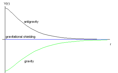
Figure 2: Gravity, antigravity and gravitational shielding in the framework of three-dimensional Einstein’s gravity with higher-derivatives.

6. DISCUSSIONS AND COMMENTS

According to a somewhat obscure unitarity lore it is expected that the operation of augmenting a non-topological massive gravity model through the topological term would transform the non-unitary systems into unitary ones and preserve the unitarity of the originally unitary models. This false idea is, perhaps, responsible for the claims in the literature concerning the pseudo-unitarity of both topologically massive Fierz-Pauli gravity (TMFPG) (Pinheiro et al., 1997a,b) and TMHDG (Pinheiro et al., 1997c). The authors of these works wrongly state that these models are unitary. As far as TMPFG is concerned, it was shown recently that this system with the Einstein’s term with the “wrong sign” is forbidden, while the model with the usual sign has acceptable mass ranges but faces ghosts problems (Deser and Tekin, 2002). On the other hand, the non-unitarity problem of TMHDG was recently rehearsed (Accioly, 2003; Accioly, 2004) and carefully tackled (Accioly and Dias, 2004b). In truth, we may say that we will never be ale to construct an unitary, massive, topologically massive, gravitational model. Indeed, the fancy way Einstein-Chern-Simons theory is built, i.e., with the Einstein’s term with the opposite sign, precludes the existence of ghost-free, massive, topologically massive, gravitational models (Accioly and Dias, 2005). It is worth mentioning that these idiosyncrasies do not occur in the framework of of massive, topologically massive, electromagnetic models because the Maxwell sign’s term concerning Maxwell-Chern-Simons theory is the same as that of the usual Maxwell’s theory.

Nonetheless, the massive topologically massive models with higher derivatives may be utilized under certain circumstance as effective field models, i.e, as low-energy approximations to more fundamental theories that, quoting Weinberg ( Weinberg, 1995), “may not be field theories at all”. The physics associated with these models is not only intriguing, but also fascinating. Certainly it deserves to be much better known.

ACKNOWLEDGMENTS

We are very grateful to Prof. S. Deser for calling our attention to the article “Massive, Topologically Massive, Models” (Deser and Tekin, 2002). A. Accioly thanks CNPq-Brazil for partial support, while M. Dias thanks CAPES-Brazil for full support.

REFERENCES

Accioly, A., Azeredo, A., and Mukai, H. (2001a). Physics Letters A 279, 169.

Accioly, A., Mukai, H., and Azeredo, A. (2001b). Classical and Quantum Gravity 18, L31.

Accioly, A., Mukai, H., and Azeredo, A. (2001c). Modern Physics Letters A 16, 1449.

Accioly, A. (2003). Physical Review D 67, 127502.

Accioly, A. (2004). Nuclear Physics B (Proceedings Supplements) 127, 100.

Accioly, A., and Dias, M. (2004a), Physical Review D 70, 107705.

Accioly, A., and Dias, M. (2004b), Modern Physics Letters A 19, 817.

Accioly, A., and Dias, M. (2005), International Journal of Modern Physics A, in press.

Antoniadis, I., and Tomboulis, E. (1986). Physical Review D 33, 2756.

Deser, S., Jackiw, R., and Templeton, S. (1982a). Physical Review Letters 48, 475.

Deser, S., Jackiw, R., and Templeton, S. (1982b). Annals of Physics 140, 372.

Deser, S., and Tekin, G. (2002). Classical and Quantum Gravity 19, L97.

Nieuwenhuizen, P. (1973). Nuclear Physics B 60, 478.

Numerov, B. (1924). Monthly Notes of the Royal Astronomical Society 84, 592.

Pinheiro, C, Pires, G., and Tomimura, N. (1996a). Il Nuovo Cimento B 111 1023.

Pinheiro, C., Pires, G., and Rabelo de Carvalho, F. (1997b). Brazilian Journal of Physics 27 14.

Pinheiro, C., Pires, G., and Sasaki, C. (1997c). General Relativity and Gravitation 29 409.

Podolsky, B., and Schwed, M. (1948). Reviews of Modern Physics 20 40.

Rivers, R. (1964). Il Nuovo Cimento 34 387.

Stelle, K. (2003). Physical Review D 16, 953.

Uspensky, J. (1948). Theory of Equations, McGraw-Hill, New York.

Weinberg., S. (1995). The Quantum Theory of Fields, Volume I, Cambridge University Press, Cambridge.