Is Schwinger Model at Finite Density a Crystal?

Abstract

It has been believed since the paper by Fischler, Kogut and SusskindSusskind that in $QED_{2}$ at finite charge density the chiral condensate exhibits a spatially inhomogeneous, oscillating behaviour. In this paper we demonstrate that this inhomogeneity is due to unphysical explicit breaking of the translational invariance by a uniform background charge density. Moreover, we investigate in the context of a simple statistical model what happens if the neutralizing background is composed instead of heavy, but dynamical, particles. We find that in contrast to the standard picture of Susskind , the chiral condensate will not exhibit coherent oscillations on large distance scales, unless the heavy neutralizing particles themselves form a crystal and the density is high.

I Introduction

Over the past years there has been a lot of interest in the phase diagram of $QCD$ at finite temperature and baryon density. The phase diagram would provide one with the answer to the childish question, “What happens to matter when you heat it up or squeeze it?” This question is relevant for the analysis of such extreme natural environments as the early universe or the dense interiors of neutron stars. The interest in the phase diagram of $QCD$ has in turn sparked studies of models of $QCD$ in non-trivial environments.

Two dimensional Quantum Electrodynamics, $QED_{2}$, commonly referred to as the Schwinger model, has served as a playground for $QCD$ theorists for many years. In the massless limit this model is exactly solvable and displays many features similar to $QCD$, most notably the generation of mass gap and the appearance of chiral condensate. The chiral condensate in this case is a manifestation of explicit chiral symmetry breaking by the axial anomaly and is generated in sectors with topological charge $\pm 1$.

The first study of the Schwinger model at finite density has been performed in Susskind . It must be noted that in this case we are talking about electric charge density, which unlike the baryon number density, is the zeroth component of a current associated with a gauged rather than global symmetry. Thus, to study $1$-flavour Schwinger model at finite density one needs to introduce background charge in order to satisfy the Gauss law. The natural choice for such a background that was adopted in Susskind is just a finite external charge uniformly smeared along the spatial direction.

The massless Schwinger model remains exactly solvable at finite density. One of its most surprising features is that once an arbitrary small charge density is introduced, the chiral condensate is no longer spatially uniform, but instead supports a plane wave structureSusskind ; Kao ,

$$\langle\bar{\psi}\psi(x)\rangle=\langle\bar{\psi}\psi\rangle_{0}\cos(2\pi\rho x+\theta)$$ (1)

where $\rho$ is the number density, $\theta$ is the topological angle of $QED_{2}$ and $\langle\bar{\psi}\psi\rangle_{0}$ denotes the chiral condensate at zero temperature, density and $\theta$ parameter. Thus, the chiral condensate experiences oscillations with the period given by inverse number density. On the other hand, as long as the quark mass is vanishing the fermion density itself is uniform. So the model does not develop a conventional crystal but rather a “chiral crystal”.

Once a finite quark mass $m$ is introduced, the non-uniformity of the chiral condensate is translated into a non-uniformity of fermion density and to leading order in $m/e$Susskind ,

$$\langle\bar{\psi}\gamma^{0}\psi(x)\rangle\approx\rho\left(1+\frac{4\pi m}{\omega^{2}}\langle\bar{\psi}\psi\rangle_{0}\cos(2\pi\rho x+\theta)\right)$$ (2)

where $\omega=e/\sqrt{\pi}$ and $e$ is the gauge coupling constant.

In this paper we will argue that the above conventional picture of oscillating chiral condensate (1) is unphysical, being a consequence of the introduction of an external static, neutralizing charge density.

There have been a number of studies of the Schwinger model at finite density both in the HamiltonianKao ; Nagy and path-integral formalismSchaposnik since the work Susskind , all of which have confirmed the oscillations of the chiral condensate. However, the ultimate reason for the breaking of the translational invariance in this model remains somewhat unclear. Indeed, one generally cannot spontaneously break continuous symmetries in $1+1$ dimensions. Moreover, the ground state of the Schwinger model at finite density is unique (once the topological $\theta$ angle is fixed) and the lowest lying excitations are separated by a mass gap $\omega$.

Yet, it is important to understand the precise reason for this phenomenon not only because it is curious by itself, but also as similar behaviour of the chiral condensate occurs in a large number of other models. In particular, both the $2d$ Gross-Neveau model and the two dimensional $QCD$ in the large $N_{c}$ limit are believed to exhibit exactly the same spatial oscillations of the chiral condensate at finite densityThies . The period of oscillations is again given precisely by the inverse fermion density. The stability of the chiral crystal against quantum fluctuations in these models is argued on the basis of the large $N_{c}$ limit: once $N_{c}=\infty$ one is allowed to circumvent the Mermin-Wagner theorem. Moreover, four-dimensional dense $QCD$ in the large $N_{c}$ limit is also expected to support a periodically modulated chiral condensateRubakov . Thus, it would be valuable to first fully understand the origin of translational symmetry breaking in $QED_{2}$, which is considerably simpler than the above zoo of models.

We demonstrate, that the reason for this phenomenon is the presence of the background charge density, which leads to the inability to simultaneously maintain invariance under translational and large gauge transformations. Alternatively, in the path integral language, translational invariance is violated by sectors with a finite topological charge. These findings naturally explain the particular form of the chiral condensate at finite density and provide a more conclusive explanation for the loss of translational invariance than those present in the literature. We show that although both the chiral and translational symmetries are explicitly broken at finite density, in the massless limit a linear combination of them remains intact, which implies,

$$\langle O(x)\rangle=e^{-\pi iq\rho x}\langle O(0)\rangle$$ (3)

where $O(x)$ is an arbitrary local operator and $q$ is the axial charge of $O$.

Having thoroughly understood the reason why the uniform background density leads to explicit breaking of translational symmetry we ask the following question. Should we consider such a theory completely sick? More precisely, does the theory with the uniform background charge ever correctly model a theory where the neutralizing charge is heavy, but dynamical. Clearly, any theory where the neutralization of charge is performed solely by dynamical fields will not exhibit explicit breaking of translational invariance. Moreover, in the absence of “special arrangements” such as $N_{c}=\infty$ the translational invariance will not be broken in two dimensions spontaneously either. However, relics of the chiral crystal might remain intact on some finite, but large, distance scale.

To answer the above question we consider a system where the neutralizing charge is modeled by dynamical classical particles of integer charge. We expect that this model corresponds to a theory where one fermion species is massless and the other is very heavy (of mass $M$), in the regime $T\ll M$, $e\ll M$, where $T$ is the temperature, provided that $T$ is sufficiently large that the quantum effects for the heavy particles can be neglected. We integrate out the light degrees of freedom (photons and massless fermions) and are left with a classical statistical mechanics model for the heavy degrees of freedom. These heavy degrees of freedom have a size of roughly $1/\omega$, interact via a Yukawa potential and should probably be identified with $B$-like mesons, consisting of one light and one heavy quark.

We find that the chiral condensate in this model will not reproduce the standard picture of Susskind (see eq. (1)), which exhibits for arbitrary density spatial oscillations with a density independent amplitude. Instead, the form of the condensate will depend crucially on the density and on the emergent dynamics of the mesons. In the regime where the model is tractable (i.e. when the mesons form a weakly interacting gas), the chiral condensate does not reproduce any of the features of eq. (1). Instead, in the dilute limit $\rho\ll\omega$, the chiral condensate is uniform and its magnitude decreases slightly with density. The correlator $\langle\bar{\psi}\frac{1+\gamma^{5}}{2}\psi(x)\bar{\psi}\frac{1-\gamma^{5}}{2}\psi(0)\rangle$ does not experience any oscillations. In the high density limit, $\rho\gg\omega$ the chiral condensate decreases exponentially with density. The correlator $\langle\bar{\psi}\frac{1+\gamma^{5}}{2}\psi(x)\bar{\psi}\frac{1-\gamma^{5}}{2}\psi(0)\rangle$ exhibits oscillations with period $\rho^{-1}$ on distance scales $x\ll\omega^{-1}$, which, however, disappear for $x\gg\omega^{-1}$. These oscillations on short distances are the only visible remnants of the chiral crystal in the gaseous regime.

Thus, we shall argue that the chiral condensate has a chance to reproduce the plane wave behaviour (1) on sufficiently large distance scales only if the density $\rho\gg\omega$ and the heavy degrees of freedom themselves are close to crystallization. Unless these specific conditions are met, the uniform background charge approximation is inapplicable and the form of the chiral condensate (1) found in Susskind ; Kao ; Schaposnik is unphysical.

II What’s Non-Uniform in a Uniform Background Density

This section is devoted to a detailed analysis of the reason for the appearance of the chiral crystal in a model with a uniform background density. The literature on this subject generally supports the following argument present in the original paperSusskind . If the spatial manifold is an infinite line ${\mathbb{R}}$, one prefers not to introduce a background charge distribution that stretches across whole of ${\mathbb{R}}$ to avoid infra-red difficulties. Instead, one chooses a background charge density to be uniform in a certain finite region of the real line (say $-L<x<L$) and zero everywhere else. Once all the calculations are done one takes $L\to\infty$. Then the “small” explicit breaking of translational symmetry present in the form of the endpoints of the charge distribution is carried by the long-range Coulomb forces across the whole system and leads to the chiral crystal structure (1).

In principal, the above invocation of the long-range forces allows one to circumvent the general theorems on the lack of spontaneous symmetry breaking in $1+1$ dimensions. However, the above argument can no longer be directly applied once the spatial manifold is compactified to a circle with the background charge uniformly smeared along its length, apparently removing the “endpoints” of the charge distribution. We adopt precisely such a compactification of the spatial coordinate in what follows.

Moreover, let us compare the situation to Schwinger model at zero density, where one observes breaking of the chiral symmetry. The modern philosophy regarding the origin of this phenomenon is that chiral symmetry is locally explicitly broken by the axial anomaly. Globally, one cannot simultaneously maintain invariance of the theory under chiral and large gauge transformations. Translating the last statement into the path integral formalism: axial charge is not conserved in non-trivial topological sectors.

We now show that a similar picture holds for the breaking of translational invariance in Schwinger model at finite density.

II.1 Hamiltonian Formalism

We start with the Lagrangian for $QED_{1+1}$,

$$L=-\frac{1}{4}F_{\mu\nu}F^{\mu\nu}+\bar{\psi}i\gamma^{\mu}D_{\mu}\psi-m\bar{\psi}\psi,\quad D_{\mu}=\partial_{\mu}-ieA_{\mu}$$ (4)

Local $U(1)$ symmetry of the theory takes the form,

$$U(1):\,\psi(x)\to e^{i\alpha(x)}\psi(x),\quad A_{\mu}(x)\to A_{\mu}(x)+\frac{1}{e}\partial_{\mu}\alpha(x)$$ (5)

For the moment we work in Minkowski space, with the conventions $\gamma^{5}=\gamma^{0}\gamma^{1}$, $\epsilon^{01}=1$. For definiteness, we take the spatial manifold to be a circle of length $L_{1}$ and pick the gauge where all fields obey periodic boundary conditions on this circle.

The energy momentum tensor for this theory is,

$$T^{\mu\nu}=\bar{\psi}i\gamma^{\mu}D^{\nu}\psi-F^{\mu\lambda}F^{\nu}_{\,\,\lambda}-g^{\mu\nu}L$$ (6)

We have not symmetrized $T^{\mu\nu}$ as it is not essential for our purposes.

Now let us couple the theory to a conserved external current $j_{ext}^{\mu}(x)$, such that $\partial_{\mu}j^{\mu}_{ext}=0$. The Lagrangian becomes,

$$L_{j}=L+j_{ext}^{\mu}A_{\mu}$$ (7)

Once this term is added, the energy momentum tensor satisfies,

$$\partial_{\mu}T^{\mu\nu}=F^{\nu\lambda}j_{\lambda\,\,ext}$$ (8)

Clearly, an external current violates the conservation of energy and momentum. Now, let us take $j^{\mu}$ to represent a uniform, neutralizing charge density,

$$j^{\mu}_{ext}=(-e\,\rho,0)$$ (9)

so that $\rho=N/L_{1}$, where $N$ is the total dynamical charge.

The equation (8) becomes,

$$\partial_{\mu}T^{\mu 0} = 0$$ (10)

$$\partial_{\mu}T^{\mu 1} = -e\,\rho\,F$$ (11)

where $F=F_{01}$, is the electric field. Thus, the uniform background charge density explicitly breaks spatial but not temporal translational invariance. In particular, defining the total momentum operator,

$$P=\int dx^{1}\,T^{01}$$ (12)

we obtain,

$$\frac{d}{dt}P=-e\,\rho\,\int dx^{1}\,F$$ (13)

If we integrate equation (13) over time,

$$\Delta P=-e\,\rho\int d^{2}x\,F$$ (14)

We recognize the integral on the righthand side of eq. (14) as the topological charge of the theory.

Thus, translational invariance is broken both locally and globally. One could try to redefine the energy momentum tensor as,

$$\hat{T}^{\mu 1}=T^{\mu 1}+e\,\rho\,\epsilon^{\mu\nu}A_{\nu}$$ (15)

and likewise the total momentum

$$\hat{P}=P+e\,\rho\int dx^{1}A_{1}$$ (16)

so that

$$\partial_{\mu}\hat{T}^{\mu 1}=0,\quad\quad\frac{d}{dt}\hat{P}=0$$ (17)

However, the local current $\hat{T}^{\mu 1}$ is clearly not a gauge invariant operator. The global object $\hat{P}$ is invariant under “small” gauge transformations characterized by $\alpha(L_{1})=\alpha(0)$, where $\alpha(x)$ is the transformation parameter of eq. (5). However, $\hat{P}$ is not invariant under large gauge transformations $U$,

$$U\psi(x^{1})U^{\dagger}=e^{2\pi ix^{1}/L_{1}}\psi(x^{1}),\quad UA_{1}U^{\dagger}=A_{1}+\frac{2\pi}{eL_{1}}$$ (18)

whereby

$$U\hat{P}U^{\dagger}=\hat{P}+2\pi\rho$$ (19)

Thus, at finite background charge density, we cannot simultaneously preserve the invariance of the theory under both translational and large gauge transformations. The usual procedure, at least at zero density, is to formulate the theory in a way, which preserves the latter symmetry and to constraint oneself to states in the Hilbert space satisfying,

$$U|\theta\rangle=e^{i\theta}|\theta\rangle$$ (20)

Then a finite translation with the operator $\hat{P}$ will take us out of the gauge invariant Hilbert space and into a different $\theta$-vacuum:

$$e^{i\hat{P}a}|\theta\rangle=|\theta+2\pi\rho a\rangle$$ (21)

Thus, for any local operator $O(x)$,

$$\langle O(x)\rangle_{\theta}=\langle O(0)\rangle_{\theta+2\pi\rho x}$$ (22)

This interplay between the $\theta$ angle and the loss of translational invariance is clear from the expressions for the chiral condensate and baryon density (1),(2). We would like to point out that we have not anywhere used the fact that our dynamical matter is fermionic. Thus, eq. (22) would remain valid in a theory with any dynamical matter fields neutralized by a uniform background charge density.

Note that a lattice subgroup of the translational group remains unbroken. Indeed, the operator,

$$S=e^{i\,\hat{P}\,\rho^{-1}}$$ (23)

is invariant under the transformation (18). But $S$ is an operator that performs translations by a distance $a=\rho^{-1}$ - the average charge spacing. Thus, our theory will respect this symmetry as can be explicitly seen from (1),(2).

The above discussion is precisely analogous to the philosophy behind the breaking of axial symmetry in $QED_{1+1}$. Recall that the gauge invariant axial current, $j^{\mu 5}=\bar{\psi}\gamma^{\mu}\gamma^{5}\psi$ suffers from an anomaly,

$$\partial_{\mu}j^{\mu 5}=-\frac{e}{2\pi}\epsilon^{\mu\nu}F_{\mu\nu}+2im\bar{\psi}\gamma^{5}\psi(x)$$ (24)

Equation (24) is an operator identity and should not be affected by infra-red effects such as temperature or finite density. Let us define the following current,

$$l^{\mu}=T^{\mu 1}-\pi\rho j^{\mu 5}$$ (25)

Observe, that $l^{\mu}$ is a gauge invariant operator, satisfying,

$$\partial_{\mu}l^{\mu}=-2\pi i\,m\,\rho\,\bar{\psi}\gamma^{5}\psi$$ (26)

So in the massless limit $m=0$,

$$\partial_{\mu}l^{\mu}=0$$ (27)

Thus, at finite density, both the axial and the translational symmetries are broken. However, in the massless limit, a linear combination of them remains intact. Defining the global charge,

$$Q=\int dx^{1}\,l^{0}(x)=P-\pi\rho Q^{5},\quad\quad\frac{d}{dt}Q=0$$ (28)

The conservation of $Q$ dictates the structure of all “non-uniformities” provided that the symmetry associated with the conservation of $Q$ is not spontaneously broken. Consider an arbitrary local operator of axial charge $q$,

$$[Q^{5},O(x)]=qO(x)$$ (29)

Then,

$$\langle O(x)\rangle=\langle\Omega|e^{-iQa}O(x)e^{iQa}|\Omega\rangle=\langle\Omega|e^{\pi i\rho aQ^{5}}O(x+a)e^{-\pi i\rho aQ^{5}}|\Omega\rangle=e^{\pi iq\rho a}\langle O(x+a)\rangle$$ (30)

$$\langle O(x+a)\rangle=e^{-\pi iq\rho a}\langle O(x)\rangle$$ (31)

In particular, for the fermion bilinear $\bar{\psi}\frac{1\pm\gamma^{5}}{2}\psi$, $q=\mp 2$ and,

$$\langle\bar{\psi}\frac{1\pm\gamma^{5}}{2}\psi(x)\rangle=e^{\pm 2\pi i\rho x}\langle\bar{\psi}\frac{1\pm\gamma^{5}}{2}\psi(0)\rangle$$ (32)

Thus, we see that the plane wave behaviour of the chiral condensate follows immediately from the structure of the theory. On the other hand, the density operator $\bar{\psi}\gamma^{0}\psi$ has $q=0$ and, therefore, does not display any non-uniformity in the massless limit. Thus, the equation (31) is in agreement with the explicit calculations of Susskind ; Kao ; Schaposnik .

Once the quark mass $m$ is non-vanishing the conservation of the current $l^{\mu}$ is explicitly broken (26). Therefore, averages of local operators no longer need to satisfy the formula (31). For instance, the fermion density $\langle\bar{\psi}\gamma^{0}\psi(x)\rangle$ becomes non-uniform as can be seen from eq. (2).

Before we conclude this section, we note that beside Schwinger model, both two dimensional chiral Gross-Neveu model and $QCD_{2}$ are believed to display the structure (31) in the large $N$ limitThies . In these theories both axial and translational symmetries are spontaneously broken, but the linear combination (28) remains preserved by the ground state. Thus, the resulting picture is the same as in Schwinger model, but the formal reason for the appearance of a chiral crystal is very different. In Schwinger model, as we have shown, translational and axial symmetries are broken explicitly (by background charge density and by chiral anomaly). In the Gross-Neveau model and $QCD_{2}$ these symmetries are broken spontaneously, with the theorems on the absence of spontaneous symmetry breaking in two dimensions circumvented due to $N=\infty$.

II.2 Path-Integral Formalism

It is instructive to understand in parallel how translational symmetry breaking is realized in the path integral formalism.

We go to Euclidean space with,

$$L_{E}=\frac{1}{4}F_{\mu\nu}F_{\mu\nu}+\bar{\psi}\gamma_{\mu}D_{\mu}\psi+m\bar{\psi}\psi$$ (33)

In our notations $\gamma_{1}\gamma_{2}=i\gamma_{5}$ , $\epsilon_{12}=1$.

We take the space-time to be a torus with $0\leq x_{1}\leq L_{1}$, $0\leq x_{2}\leq L_{2}$. Physically, $L_{2}=\beta=T^{-1}$ is the inverse temperature. Gauge fields on a torus fall apart into sectors classified by the topological charge,

$$n=\frac{e}{2\pi}\int d^{2}x\,F$$ (34)

where $F=F_{12}$. In a general topological sector, the gauge and fermion fields are not strictly periodic, but satisfy,

$$\psi(x_{1},L_{2})=V_{1}(x_{1})\psi(x_{1},0),\quad A_{\mu}(x_{1},L_{2})=A_{\mu}(x_{1},0)-\frac{i}{e}\partial_{\mu}V_{1}(x_{1})V_{1}^{\dagger}(x_{1})$$ (35)

$$\psi(L_{1},x_{2})=V_{2}(x_{2})\psi(0,x_{2}),\quad A_{\mu}(L_{1},x_{2})=A_{\mu}(0,x_{2})-\frac{i}{e}\partial_{\mu}V_{2}(x_{2})V_{2}^{\dagger}(x_{2})$$ (36)

with $V_{1}$, $V_{2}$ satisfying the consistency conditions,

$$V_{1}(0)V_{2}(L_{2})=V_{2}(0)V_{1}(L_{1})$$ (37)

The transition functions $V_{1},V_{2}$ in turn determine the topological charge $n$.

For each $n$, we have some gauge freedom in choosing $V_{1},V_{2}$. For instance, one choice is to have fermions anti-periodic in the temporal ($x_{2}$) direction, so that,

$$V_{1}(x_{1})=-1,\quad V_{2}(x_{2})=e^{2\pi inx_{2}/L_{2}}$$ (38)

Let us recall that an external heavy static particle is inserted into the theory in the form of a temporal Wilson loop. For instance, the partition function in the background of $m$ static charges located at points $\{x_{i}\}$ and with charges $\{e\,p_{i}\}$, $p_{i}\in{\mathbb{Z}}$ is,

$$Z=\int\,{\cal D}A{\cal D}\bar{\psi}{\cal D}\psi\,\prod_{i=1}^{m}W(x_{i},p_{i})\,e^{-S}e^{in\theta}$$ (39)

with

$$W(x,p)=\left(-V_{1}(x_{1})^{-1}e^{ie\int A_{2}(x,\tau)d\tau}\right)^{p}$$ (40)

We have inserted the prefactor $(-1)^{p}$, so that in a gauge where $V_{1}(x_{1})=-1$, $W(x,p)$ reduces to the standard form,

$$W(x,p)=\exp(ip\,e\int A_{2}(x,\tau)d\tau)$$ (41)

Expression (40) is completely gauge invariant and geometrically is the transport with respect to $A$ along a temporal cycle, taken in representation $p$ of the $U(1)$ group.

It is clear that once $p$ ceases to be an integer the expression (40) for $W(x,p)$ becomes ambiguous (the only representations of the $U(1)$ group are integral). This is not surprising - it is precisely for this reason that the existence of monopoles enforces quantization of electric charge. In the present case the role of monopoles is played by $2d$ instantons. Similarly, it is problematic to generalize the prefactor in $W$ involving the transition functions $V$ to a continuous background charge distribution in a manifestly gauge invariant manner.

We may still attempt to take the limit of a continuous charge distribution in a particular gauge. The choice $V_{1}(x_{1})=-1$ seems to be most suited for this purpose. As noted above, as long as we are working with integral charges in this gauge, the transition functions drop out of expression (40). Now we can take the “continuum” limit,

$$Z=\int\,{\cal D}A{\cal D}\bar{\psi}{\cal D}\psi\,e^{ie\int d^{2}x\,j^{ext}_{2}A_{2}}\,e^{-S}e^{in\theta}$$ (42)

where $j^{ext}_{2}(x_{1})$ is the static background charge density and (anti)periodic temporal boundary conditions on (fermions) gauge fields are assumed from here on. Expression (42) is not invariant under gauge transformations, which change these boundary conditions.

Now let us address the question of translational symmetry breaking. First, to understand the root of the problem consider a fractional charge $p$ situated at $x_{1}=L_{1}^{-}$ and move it across the artificial cut at $x_{1}=0\sim L_{1}$ to $x_{1}=0^{+}$. Observe,

$$W(L_{1},p)=e^{iep\int A_{2}(L_{1},\tau)d\tau}=e^{iep\int A_{2}(0,\tau)d\tau}e^{p\int\partial_{2}V_{2}(\tau)V^{\dagger}_{2}(\tau)}=e^{2\pi ipn}W(0,p)$$ (43)

Thus, the cut on the torus is visible to a fractional charge and invisible to an integer charge. Of course, there is nothing new in this result. However, it is precisely this fact that leads to translational symmetry breaking.

Indeed, take an arbitrary local operator $O(x)$ and pick $a>0$ such that $0<x,x+a<L_{1}$. Let us compute the expectation value of $O(x)$ in the background of the charge distribution $j^{ext}_{2}$. Then,

$$\langle O(x+a)\rangle=\frac{1}{Z}\int\,{\cal D}A{\cal D}\bar{\psi}{\cal D}\psi\,O(x+a)e^{ie\int d^{2}x\,j^{ext}_{2}A_{2}}\,e^{-S}e^{in\theta}$$ (44)

We make the following change of variables,

$$\psi^{\prime}(x_{1},x_{2}) = \psi(x_{1}+a,x_{2}),\,A^{\prime}_{\mu}(x_{1},x_{2})=A_{\mu}(x_{1}+a,x_{2}),\,0<x_{1}<L_{1}-a$$ (45)

$$\psi^{\prime}(x_{1},x_{2}) = V_{2}(x_{2})\psi(x_{1}+a-L_{1},x_{2}),\,L_{1}-a<x_{1}<L_{1}$$ (46)

$$\,A^{\prime}_{\mu}(x_{1},x_{2}) = A_{\mu}(x_{1}+a-L_{1},x_{2})-\frac{i}{e}\partial_{\mu}V_{2}(x_{2})V^{\dagger}_{2}(x_{2}),\,L_{1}-a<x_{1}<L_{1}$$ (47)

It is easy to see that $\psi^{\prime}$, $A^{\prime}$ obey the same boundary conditions as original variables $\psi$, $A$. Thus,

$$\langle O(x+a)\rangle=\frac{1}{Z}\int\,{\cal D}A^{\prime}{\cal D}\bar{\psi^{\prime}}{\cal D}\psi^{\prime}\,O^{\prime}(x)e^{-2\pi in\int_{0}^{a}dx_{1}j^{ext}_{2}(x_{1})}e^{ie\int d^{2}x\,j^{\prime ext}_{2}A^{\prime}_{2}}\,e^{-S}e^{in\theta}$$ (48)

where

$$j^{\prime ext}_{2}(x_{1})=\left\{\begin{array}[]{ll}j^{ext}_{2}(x_{1}+a)&0<x_{1}<L_{1}-a\\ j^{ext}_{2}(x_{1}+a-L_{1})&L_{1}-a<x_{1}<L_{1}\end{array}\right.$$ (49)

is just the properly shifted background charge density. Thus, we get an extra factor,

$$e^{-2\pi in\int_{0}^{a}dx_{1}j^{ext}_{2}(x_{1})}$$ (50)

related to the amount of charge passing through the cut during our translation. As long as this charge is an integer, the factor (50) is unity and the cut is invisible.

Now suppose our background charge is uniformly smeared across the spatial circle, $j^{ext}_{2}(x_{1})=-\rho$, where $\rho=\frac{N}{L_{1}}$ is the dynamical charge. The background charge density itself is invariant under shifts along the circle, $j^{\prime ext}_{2}=j^{ext}_{2}$ and the factor (50) becomes, $e^{2\pi in\rho a}$. Hence,

$$\langle O(x+a)\rangle_{\theta}=\langle O(x)\rangle_{\theta+2\pi\rho a}$$ (51)

in agreement with (22). Moreover, if we disentangle the contributions to $\langle O(x)\rangle$ coming from distinct topological sectors,

$$\langle O(x)\rangle_{n}=e^{2\pi in\rho x}\langle O(0)\rangle_{n}$$ (52)

Thus, different topological sectors contribute to $\langle O(x)\rangle$ with different “harmonics.” One effect of (52) is that only the topologically trivial $n=0$ sector contributes to the partition function and the topological susceptibility vanishes even if the quark mass $m$ is non-zero.

Finally, if the quark mass is vanishing then due to fermion zero modes, operators with axial charge $q$ get a contribution only from sectors with $n=-\frac{q}{2}$. Thus, for $m=0$,

$$\langle O(x)\rangle=e^{-\pi iq\rho x}\langle O(0)\rangle$$ (53)

in agreement with (31).

Before we conclude this section, we would like to note that in the massless limit explicit calculations can be done for the theory defined by (42) on a finite torus. These are summarized in the appendix. In particular,

$$\langle\bar{\psi}\frac{1+\gamma^{5}}{2}\psi(x)\rangle=\frac{1}{2}e^{i\theta}e^{2\pi i\rho x}\langle\bar{\psi}\psi\rangle_{L_{1},L_{2}}$$ (54)

where $\langle\bar{\psi}\psi\rangle_{L_{1},L_{2}}$ is the chiral condensate at zero density and $\theta$ parameter on the torus of dimensions $L_{1},L_{2}$. The result (54) generalizes the path-integral computation of Schaposnik , which was performed on an infinite Euclidean space to the case of a finite torus, where all the infra-red singularities are under complete control. Technically, the oscillating factor $e^{2\pi i\rho x}$ comes from averaging the fermion zero mode over torons (constant parts of field $A_{\mu}(x)=t_{\mu}$) in the presence of background charge.

III Dynamical Background

III.1 General Remarks

In the previous section we saw that a uniform background charge density explicitly breaks translational invariance. This effect may seem to be rather unphysical, in particular as it has to do with the Dirac string being visible to our background charge. But after all, the uniform background density is typically taken to model some heavy, but dynamical, particles. Once all fields are dynamical, it is clear that translational symmetry is not explicitly broken. However, one would like to ask whether any features of the chiral crystal discussed in the previous section remain.

To answer the above question, we would like to analyze $QED_{2}$ with two flavours. We take one fermion flavour to have charge $e$ and vanishing mass and the other flavour to have charge $qe$, $q\in{\mathbb{N}}$ and mass $M\gg e$. We want to analyze the problem at a finite “isospin” density, with the heavy fermions neutralizing the light ones. We work at finite temperature $T$. We will treat the problem in a “Born-Oppenheimer” like approximation. Namely, we first freeze the positions of heavy particles, treating them as static external charges, and integrate over the light fermions and gauge fields. For instance, the partition function of the system in the background of $N$ external charges situated at points $\{{x_{i}}\}$ is,

$$Z(x_{1},..x_{N})=\langle\prod_{i}W(x_{i},-q)\rangle_{l}$$ (55)

where the subscript $l$ denotes integration over the light degrees of freedom. We then promote the external charges to dynamical degrees of freedom, treating them as classical particles. For example, the full partition function takes the form,

$$Z=\sum^{\infty}_{n=0}\frac{z^{n}}{n!}\int dx_{1}..dx_{n}\langle\prod_{i}W(x_{i},-q)\rangle_{l}$$ (56)

Here $z=\frac{1}{\lambda}e^{\beta(\mu-M)}$ is the activity, $\mu$ is the chemical potential and $\lambda=(\frac{2\pi}{MT})^{\frac{1}{2}}$ is the thermal wavelength. Similarly, the expectation value of some operator $O$ involving light quark fields is,

$$\langle O\rangle=\frac{1}{Z}\sum^{\infty}_{n=0}\frac{z^{n}}{n!}\int dx_{1}..dx_{n}\langle O\,\prod_{i}W(x_{i},-q)\rangle_{l}$$ (57)

We will often use the notation,

$$\langle O\rangle_{\{x_{i},q_{i}\}}=Z^{-1}(x_{1},..x_{n})\langle O\prod_{i}W(x_{i},q_{i})\rangle_{l}$$ (58)

We shall shortly see that after integration over the light degrees of freedom, the heavy fermions get dressed into meson like particles, consisting (in terms of quantum numbers) of $q$ light and one heavy quark. So the effective theory (56) should be understood as describing classical dynamics of such mesons. We expect such an approximation to be valid as long as $M\gg e,M\gg T$ so that the heavy quark-antiquark pairs do not get excited either virtually or thermally. Moreover, we need $T$ to be high enough that the meson gas/liquid is in a classical rather than quantum regime. In the dilute gas limit, we expect that the system can be treated classically for $T\gg\frac{\rho^{2}}{2M}$.

As a first step to analyze the resulting system, we need to perform the integration over the light fermions and gauge fields. We shall work on a Euclidean torus of spatial and temporal lengths $L_{1}$, $L_{2}=T^{-1}$. The expectation value of a product of straight temporal Wilson loops in the massless Schwinger model has been computed in a number of worksGordon ; Zahed . The result is (see the appendix for a sketch of the calculation),

$$\langle\prod_{i}W(x_{i},q_{i})\rangle_{l} = \exp\left(-L_{2}\,\frac{1}{2}\sum_{i,j}q_{i}q_{j}e^{2}V(x_{i}-x_{j})\right)$$ (59)

$$V(x) = \frac{1}{L_{1}}\sum_{p_{1}}\frac{1}{p^{2}_{1}+\omega^{2}}\,e^{ip_{1}x}\,\stackrel{{\scriptstyle L_{1}\to\infty}}{{=}}\frac{1}{2\omega}e^{-\omega|x|}$$ (60)

where $\omega=e/\sqrt{\pi}$ and $p_{1}=2\pi m/L_{1}$, $m\in Z$. Thus, our heavy particles (of like charge) interact via a two-body repulsive Yukawa potential with all three and higher particle interactions vanishing. It is also instructive to compute the charge density of light quarks,

$$\langle\bar{\psi}\gamma_{2}\psi(x)\rangle_{\{x_{i},q_{i}\}}=-\frac{1}{\pi}\sum_{i}q_{i}V(x-x_{i})$$ (61)

It is clear from (61) that each heavy quark of charge $-q$ is surrounded by a cloud of light quarks with a radius of roughly $\omega^{-1}$. The cloud has total charge $q$ that screens the Coulomb potential of the heavy quark producing a meson, similar to the heavy-light mesons of $QCD$ (such as the $B$-meson).

We will be most interested in the expectation value of the chiral condensate $\langle\bar{\psi}\frac{1+\gamma^{5}}{2}\psi\rangle$. For static sources this is given byZahed (we sketch the calculation in the appendix),

$$\langle\bar{\psi}\frac{1+\gamma^{5}}{2}\psi(x)\rangle_{\{x_{i},q_{i}\}}=\frac{1}{2}e^{i\theta}\langle\bar{\psi}\psi\rangle_{L_{1},L_{2}}\prod_{i}\left(U(x-x_{i})\right)^{-q_{i}}$$ (62)

where

$$U(x)=\exp(2\pi iV^{\prime}(x))\stackrel{{\scriptstyle L_{1}\to\infty}}{{=}}\exp(-\pi isgn(x)e^{-\omega|x|})$$ (63)

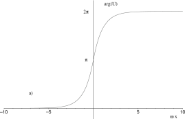
Figure 1: a) The phase of the chiral condensate $\arg U(x)=\arg\langle\bar{\psi}\frac{1+\gamma^{5}}{2}\psi(x)\rangle$ in the background of a static unit charge placed at $x=0$ for $\theta=0$. b) The chiral condensate in units of $\langle\bar{\psi}\psi\rangle_{T}$ in the background of two widely separated static unit charges for $\theta=0$.

Thus, the introduction of static charges only affects the phase of the chiral condensate. Moreover, $U(x)\to 1$ for $|x|\gg\omega^{-1}$, so each static charge affects the chiral condensate only in a region of radius roughly $\omega^{-1}$ - the size of the meson. Notice that $U(x)$ makes one loop on the unit circle in the complex plane as $x$ winds around the spatial circle (see Fig. 1 a)). Thus, the phase of the condensate (62) winds by $2\pi N$ as $x$ moves around the spatial circle, where $N=-\sum_{i}q_{i}$ is the total charge of the light fermions. So, the total winding number of $\langle\bar{\psi}\frac{1+\gamma^{5}}{2}\psi(x)\rangle_{\{x_{i},q_{i}\}}$ is independent of the positions of the heavy quarks and, in fact, is the same as for the model with the uniform background charge density (54). However, the winding occurs in the vicinity of the heavy charges, over the radius of each meson, as opposed to the uniform background case, where the winding is uniformly smeared across the whole system. We expect this difference to be particularly important in the dilute limit $\rho\ll\omega$ when the distance between mesons is much larger than their size. In this regime, each meson keeps its individual features and $\langle\bar{\psi}\psi\rangle_{\{x_{i},-q\}}\to\langle\bar{\psi}\psi\rangle_{T}\cos(\theta)$ in the wide regions between the mesons (see Fig. 1 b)). Here, $\langle\bar{\psi}\psi\rangle_{T}$ is the infinite volume limit of the chiral condensate at zero density and $\theta$ parameter and finite temperature $T$. Thus, the uniform background approximation is expected to fail badly in the dilute regime.

It is instructive to see what happens to the chiral condensate if we arrange our heavy charges into a regular lattice, $x_{j}=ja$, $q_{j}=-q$. Using (62) and taking $L_{1}\to\infty$,

$$\langle\bar{\psi}\frac{1+\gamma^{5}}{2}\psi(x)\rangle_{\{x_{i},q_{i}\}}=\frac{1}{2}e^{i\theta}\langle\bar{\psi}\psi\rangle_{T}\,e^{i\phi(x)}$$ (64)

where $\phi(x)$ is a periodic function with period $x=a$ and,

$$\phi(x)=\pi q\frac{\sinh(\omega(x-a/2))}{\sinh(\omega a/2)},\quad 0<x<a$$ (65)

For $\omega a\gg 1$ we have a crystal of widely spaced mesons much like on Fig. 1 b). In the high density limit, $\omega a\ll 1$, the screening clouds of heavy charges overlap and the individual mesons are washed out. Instead, we may approximate,

$$\phi(x)\approx 2\pi q\,\left(\frac{x}{a}-\frac{1}{2}\right),\quad 0<x<a$$ (66)

so that,

$$\langle\bar{\psi}\frac{1+\gamma^{5}}{2}\psi(x)\rangle_{\{x_{i},q_{i}\}}=\frac{1}{2}e^{i\theta}(-1)^{q}e^{2\pi i\rho x}\langle\bar{\psi}\psi\rangle_{T}$$ (67)

where $\rho=q/a=N/L$. Thus, in this limit we recover the uniform background approximation (54). However, note that the existence of coherent, long-range, oscillations of the chiral condensate (67) is possible only if the dynamics governing the heavy charges are such that they organize a crystal-like state. For a one-dimensional statistical system interacting with a finite range potential (60) a true crystal cannot form. However, the system may exhibit crystal order on some finite distance scale $d\gg\omega^{-1}$. In this case, we expect that the plane wave behaviour of the chiral condensate will also persist on the same distance scale $d$. Otherwise, if the mesons form a disordered, weakly-interacting gas the oscillations (67) will be washed out on distance scales $x\gg\omega^{-1}$, as we shall show shortly.

In fact, equation (62) suggests that the external charges act as impurities, whose effect is to disorder the chiral condensate. If the impurities are in a weakly interacting regime, the disorder is “random”. This is precisely the situation that we will analyze in the next section.

III.2 Statistical Model

Let us now make the heavy charges dynamical and analyze the statistical model (56). Our main objective is to compute the chiral condensate (57),(62),

$$\langle\bar{\psi}\frac{1+\gamma^{5}}{2}\psi(x)\rangle = \frac{1}{2}e^{i\theta}\langle\bar{\psi}\psi\rangle_{T}\frac{1}{Z}\sum_{n=0}^{\infty}\frac{z^{n}}{n!}\int dx_{1}..dx_{n}\prod_{i}U(x-x_{i})^{q}\exp(-\frac{\beta}{2}\sum_{ij}q^{2}e^{2}V(x_{i}-x_{j}))$$ (68)

$$= \frac{1}{2}e^{i\theta}\langle\bar{\psi}\psi\rangle_{T}\sum_{n=0}^{\infty}\frac{1}{n!}\int dx_{1}..dx_{n}\prod_{i}(U(x-x_{i})^{q}-1)g_{n}(x_{1},..x_{n})$$

where $g_{n}(x_{1},..x_{n})$ is the $n$-point correlation function,

$$g_{n}(x_{1},..x_{n})=z^{n}\frac{1}{Z}\sum_{m=0}^{\infty}\frac{z^{m}}{m!}\int dx_{n+1}..dx_{n+m}\exp(-\frac{\beta}{2}\sum_{ij=1}^{n+m}q^{2}e^{2}V(x_{i}-x_{j}))$$ (69)

Notice that the chiral condensate is sensitive only to short-distance properties of the correlation functions $g_{n}(x_{1}..x_{n})$ as the range of $U(x)^{q}-1$ is roughly $\omega^{-1}$.

We would like to perform the Meyer expansion in activity $z$. The leading term in the equation of state, as always, is,

$$\beta P=z^{*}$$ (70)

where $P$ is the pressure and $z^{*}=z\exp(-\frac{1}{2}{\beta}q^{2}e^{2}V(0))$ ($z^{*}$ includes the self-interaction energy of each meson). Then,

$$\rho_{h}=z\frac{\partial}{\partial z}(\beta P)=z^{*}$$ (71)

where $\rho_{h}$ is the density of heavy particles,

$$q\rho_{h}=\rho$$ (72)

As the range of the potential $V$ is $\omega^{-1}$ and strength $e^{2}V\sim\omega$, the corrections to the equation of state for $T\sim\omega$ are suppressed in the Meyer cluster expansion by powers of $z^{*}/\omega$. So for, $\rho\ll\omega$, $T\sim\omega$ our system behaves like a weakly-interacting gas of mesons. Moreover, in this regime, at leading order the $n$ point function on distances $x\sim\omega^{-1}$ scales as ${z^{*}}^{n}$ so that terms in (68) involving $g_{n}(x_{1},..x_{n})$ are suppressed by $(z^{*}/\omega)^{n}$. The leading correction to the chiral condensate comes from the $n=1$ term. Recalling, $g_{1}(x)=\rho_{h}$,

$$\langle\bar{\psi}\frac{1+\gamma^{5}}{2}\psi\rangle\approx\frac{1}{2}e^{i\theta}\langle\bar{\psi}\psi\rangle_{T}(1+\rho_{h}\int dx(U(x)^{q}-1))$$ (73)

Performing the integral,

$$\langle\bar{\psi}\psi\rangle\approx(1-\frac{\rho_{h}}{\omega}u(q))\langle{\bar{\psi}\psi}\rangle_{T}\cos(\theta)$$ (74)

where,

$$u(q)=2\int_{0}^{\pi q}dt\frac{(1-\cos(t))}{t}=2(\log(\pi q)+\gamma-Ci(\pi q))$$ (75)

Thus, we have calculated the first correction in density to the chiral condensate in the regime of a weakly interacting dilute meson gas. The result (74) is reminiscent of the behaviour of the chiral condensate in $N_{c}=2$ $QCD$ at small baryon densityKSTVZ , in $N_{c}=3$ $QCD$ at small isospin densitySS and in the “dilute” nuclear matternuclear . In all of these theories, one thinks of the system as being composed of a dilute gas of particles $M$ (diquarks for $N_{c}=2$ $QCD$, pions for $N_{c}=3$ $QCD$, nuclons for nuclear matter) and obtains,

$$\langle\bar{\psi}\psi\rangle_{\rho}\approx\langle\bar{\psi}\psi\rangle_{0}+\rho\langle M|\bar{\psi}\psi|M\rangle$$ (76)

where $|M\rangle$ is a one particle state in vacuum (with normalization $\langle M(p)|M(p^{\prime})\rangle=(2\pi)^{d}\delta^{d}(p-p^{\prime})$). So, we identify,

$$\langle q|\bar{\psi}\psi|q\rangle_{T,\theta}=\int dx(U(x)^{q}-1)\,\langle\bar{\psi}\psi\rangle_{T}\cos(\theta)=-\frac{1}{\omega}u(q)\langle\bar{\psi}\psi\rangle_{T}\cos(\theta)$$ (77)

where $|q\rangle$ denotes our heavy-light meson state.

So far we have concentrated on the region $T\sim\omega$ where the criterion for the applicability of Meyer’s expansion was $\rho\ll\omega$. Now, let’s analyze the low temperature regime $T\ll\omega$. In this case, the interaction effectively becomes hardcore of range $\omega^{-1}\log(\omega/T)$, so for the Meyer expansion to be valid, we need $z^{*}\ll\omega/\log(\omega/T)$. If this condition is satisfied, the chiral condensate at leading order in $\rho$ is again given by (74). Moreover, we actually expect the expressions (74), (77) to remain valid in a wider range $\rho\ll\omega$ down to the extreme quantum regime at $T=0$, based on general phase-space arguments.

Finally, let’s study the high-temperature regime $T\gg\omega$. In this case, it can be shown that the corrections to the ideal gas equation of state (70) are suppressed by powers of $z/T$. In particular, if $\omega\ll\rho\ll T$ we are still in the weakly interacting (but not dilute!) regime. In this case it is convenient to rewrite (68) as,

$$\langle\bar{\psi}\frac{1+\gamma^{5}}{2}\psi(x)\rangle=\frac{1}{2}e^{i\theta}\langle\bar{\psi}\psi\rangle_{T}\exp\left(\sum_{n=1}^{\infty}\frac{1}{n!}\int dx_{1}..dx_{n}\prod_{i}(U(x-x_{i})^{q}-1)g_{n}(x_{1},..x_{n})_{conn}\right)$$ (78)

where $g_{n}(x_{1},..x_{n})_{conn}$ denotes the fully connected $n$-point correlation function. It is easy to show that the terms in the exponent involving the $n$-point correlation function are suppressed by $(z/T)^{n-1}$ compared to the leading term and,

$$\langle\bar{\psi}\psi\rangle\approx\exp\left(-\frac{\rho_{h}}{\omega}u(q)\right)\langle\bar{\psi}\psi\rangle_{T}\cos(\theta)$$ (79)

The expression (79) agrees with (74) in the dilute limit $\rho\ll\omega$. In the dense gas limit, $\omega\ll\rho\ll T$, the chiral condensate exponentially decreases with density. Note that for $T\gg\omega$ the chiral condensate at zero density is already exponentially suppressed with temperature compared to $T=0$ (see eq. (119)).

III.3 Correlation Functions

To answer the question of whether any remnants of the oscillating behaviour (54) exist in our model, the computation of the chiral condensate presented in the previous section is not sufficient. Indeed, translational invariance implies that the chiral condensate is uniform. Instead, we must compute the static correlation function, $\langle S_{+}(x)S_{-}(y)\rangle$, $S_{\pm}(x)=\bar{\psi}\frac{1\pm\gamma_{5}}{2}\psi(x)$. We would like to see on what distance scales this correlation function exhibits plane wave structure (54). Integrating out light degrees of freedom,

$$\langle S_{+}(x)S_{-}(y)\rangle_{\{x_{i},q_{i}\}}=S(x-y)\prod_{i}(U(x-x_{i}))^{-q_{i}}(U(y-x_{i}))^{q_{i}}$$ (80)

where,

$$S(x-y) = \langle S_{+}(x)S_{-}(y)\rangle_{L_{1},L_{2}}=\frac{1}{4}|\langle\bar{\psi}\psi\rangle_{L_{1},L_{2}}|^{2}e^{4\pi G_{\omega}(x-y)}$$ (81)

$$\quad G_{\omega}(x) = \frac{1}{L_{1}L_{2}}\sum_{p}\frac{1}{p^{2}+\omega^{2}}e^{ipx},\quad p=\left(\frac{2\pi m_{1}}{L_{1}},\frac{2\pi m_{2}}{L_{2}}\right),\,m_{1},m_{2}\in{\mathbb{Z}}$$ (82)

Thus,

$$\langle S_{+}(x)S_{-}(y)\rangle=S(x-y)F(x-y)$$ (83)

$$F(x-y)=\exp\left(\sum_{n=1}^{\infty}\frac{1}{n!}\int dx_{1}..dx_{n}\prod_{i}(U(x-x_{i})^{q}U(y-x_{i})^{-q}-1)g_{n}(x_{1},..x_{n})_{conn}\right)$$ (84)

So the correlation function factorizes into two pieces. The first, $S(x-y)$, is just the correlation function in vacuum. The second, $F(x-y)$, contains the finite density information.

As noted in the previous section, in the regime where the Meyer expansion is applicable, we may truncate the series in the exponent of (85) at the leading ($n$ = 1) term,

$$F(x-y)=e^{{\rho_{h}}f(x-y)}$$ (85)

where,

$$f(x-y)=\int dx_{1}(U(x-x_{1})^{q}U(y-x_{1})^{-q}-1)$$ (86)

The function $f(x)$ is plotted in Fig. 2.

Figure 2: Function $f(x)$ that enters the correlator $\langle S_{+}(x)S_{-}(0)\rangle$ (see eqs. (83), (85)). Here we chose $q=1$.

It is easy to see that for $|x-y|\gg\omega^{-1}$,

$$f(x-y)\to\int dx_{1}(U(x-x_{1})^{q}-1)+\int dx_{1}(U(y-x_{1})^{-q}-1)=-\frac{2}{\omega}u(q)$$ (87)

Thus, $\langle S_{+}(x)S_{-}(y)\rangle$ will not exhibit oscillations (54) for $|x-y|\gg\omega^{-1}$.

Note that $S(x-y)\to\frac{1}{4}|\langle\bar{\psi}\psi\rangle_{T}|^{2}$ for $|x-y|\to\infty$ so,

$$\langle S_{+}(x)S_{-}(y)\rangle\stackrel{{\scriptstyle|x-y|\to\infty}}{{=}}\frac{1}{4}|\langle\bar{\psi}\psi\rangle_{T}|^{2}\exp(-2\frac{\rho_{h}}{\omega}u(q))=\langle S_{+}\rangle\langle S_{-}\rangle$$ (88)

and the correlation function clusters.

We may also investigate the short distance behaviour. Expanding $f(x)$ in a Taylor series in $\omega x$,

$$f(x)=\frac{1}{\omega}(2\pi iq\omega x-\frac{1}{2}\pi^{2}(q\omega x)^{2}+...)$$ (89)

Hence, for $|x|\ll\omega^{-1}$,

$$\langle S_{+}(x)S_{-}(0)\rangle\approx\exp(2\pi i\rho x-\frac{\pi^{2}q}{2}\frac{\rho}{\omega}(\omega x)^{2})S(x)$$ (90)

The above equation clearly exhibits the plane wave behaviour with period $x=\rho^{-1}$. However, recall that eq. (90). is valid only for $|x|\ll\omega^{-1}$. Thus, in the dilute limit $\rho\ll\omega$, no full oscillations appear and, in fact, eqs. (83),(85) are more appropriately written as,

$$\langle S_{+}(x)S_{-}(0)\rangle=(1+\rho_{h}f(x))S(x)$$ (91)

In the dense gas regime, $\rho\gg\omega$, the oscillations are, indeed, present on short distance scales, however, as eq. (90) shows, they become damped for $x\gtrsim(\frac{\omega}{\rho})^{\frac{1}{2}}\omega^{-1}$ and disappear altogether for $x\gg\omega^{-1}$. Moreover, these oscillations modulate the zero-density correlator $S(x)$, which itself has a quite non-trivial behaviour for distances $x\lesssim\omega^{-1}$.

IV Conclusion

In this paper we have analyzed some puzzles related to the Schwinger model at finite density. We have shown that the well-known plane-wave behaviour of the chiral condensate is a consequence of explicit breaking of translational invariance by a background charge density. Similarly to the non-conservation of axial charge, the non-conservation of total momentum is globally saturated in sectors of non-trivial topological charge. In fact, the breaking of translational symmetry at finite density is a much simpler phenomenon than the breaking of chiral symmetry by the anomaly as the former appears already on the classical level, while the later is a purely quantum phenomenon.

In the second part of this paper, we have explored the question: “What happens if the uniform background density is replaced by a dynamical, but heavy, field?” To answer this question, we have analyzed a statistical model in which the heavy neutralizing charge comes from an ensemble of classical particles. We have shown that the effect of heavy charges is to disorder the chiral condensate. In the regime where the gas of heavy charges is almost ideal, the chiral condensate is spatially uniform and decreasing with density. For the charge density $\rho\ll\omega$ the “disorder” is weak and we compute the leading density correction to the chiral condensate (74). In the dense gas regime $\rho\gg\omega$ the disorder leads to an exponential suppression of the chiral condensate. In both of these regimes, the condensate does not exhibit any oscillations on distance scales $x\gg\omega^{-1}$, as is clear from computing the correlator $\langle S_{+}(x)S_{-}(0)\rangle=\langle\bar{\psi}\frac{1+\gamma^{5}}{2}\psi(x)\bar{\psi}\frac{1-\gamma^{5}}{2}\psi(0)\rangle$. The only remnant of oscillatory behaviour comes at high density $\rho\gg\omega$ in the short distance behavior of $\langle S_{+}(x)S_{-}(0)\rangle$ for $x\ll\omega^{-1}$.

In fact, we have argued that the only way for the oscillations to survive on distance scales larger than $\omega^{-1}$ is for the system to be in the high density regime $\rho\gg\omega$ and the heavy charges to crystalize. In the dilute regime, $\rho\ll\omega$ we do not expect to recover the oscillatory behaviour even if the heavy charges were to crystalize.

So clearly the uniform background approximation generically does not accurately model the situation where the neutralizing charge is dynamical, rendering the results of Susskind ; Kao ; Schaposnik unphysical. Indeed, we expect such an approximation to work well if the light and heavy neutralizing charges are largely decoupled from each other (e.g. valence electrons in a metal). However, in the Schwinger model the light fermions are very strongly coupled to the neutralizing charges producing heavy-light mesons. The approximation fails particularly badly in the dilute phase, where the distance between the mesons is much larger than their size. To apply the uniform background charge approximation here would be akin to treating the nucleii in a dilute atomic gas as uniform.

We conclude by noting that we certainly have not analyzed the entire phase-diagram of the two-flavour heavy-light Schwinger model. We have treated the gas of heavy-light mesons classically and have not touched upon the quantum regime at all. Neither have we analyzed the regime where the classical system is far from an ideal gas limit and the interactions between mesons are important. These regimes are subject to further investigation and, in fact, have a higher chance of exhibiting the plane-wave behaviour of chiral condensate on distance scales larger than $\omega^{-1}$ than the “random disorder” case considered here.

Appendix A Explicit Calculation of the Chiral Condensate at Finite Density

The purpose of this appendix is to perform the calculation of the partition function and chiral condensate at finite background charge density on a Euclidean torus. In case when the background charge is in the form of discrete charges (Wilson loops) this computation has been performed beforeGordon ; Zahed . For a uniform background charge density, the calculation has been done on an infinite Euclidean planeSchaposnik . Here, we keep the size of our torus finite throughout the calculation, gaining complete control of all the infra-red subtleties. For a detailed study of the Schwinger model on the torus (at zero density) see Azakov .

We work in a gauge where the (fermion) gauge fields are (anti) periodic in the temporal direction, with the transition functions (38),

$$V_{1}(x_{1})=-1,\quad V_{2}(x_{2})=e^{2\pi inx_{2}/L_{2}}$$ (92)

We decompose the gauge fields as,

$$A_{\mu}=t_{\mu}+\partial_{\mu}\alpha+\epsilon_{\mu\nu}\partial_{\nu}b+A^{n}_{\mu}$$ (93)

where $\alpha$ and $b$ are both periodic fields on the torus orthogonal to unity ($\int d^{2}x\,\alpha=\int d^{2}x\,b=0$). The variable $t_{\mu}$ is the so-called toron field and plays a crucial part in all the calculations. $t_{\mu}$ is effectively an angular variable, with $t_{\mu}\sim t_{\mu}+\frac{2\pi m}{eL_{\mu}},\,m\in{\mathbb{Z}}$. We shall consider only the case where the total background charge is integral, $\int dx_{1}j_{2}^{ext}(x_{1})=-N,\,N\in{\mathbb{Z}}$ so that the angular nature of $t_{\mu}$ is unspoiled. $A^{n}_{\mu}$ is the “instanton” field in the $n$-th topological sector. We choose,

$$A^{n}_{1}=0,\quad A^{n}_{2}=\frac{2\pi nx_{1}}{eL_{1}L_{2}}$$ (94)

which obeys the periodicity conditions (35),(36).

First, let’s compute the partition function,

$$Z=\int\,{\cal D}A{\cal D}\bar{\psi}{\cal D}\psi\,e^{ie\int d^{2}x\,j^{ext}_{2}A_{2}}\,e^{-S}e^{in\theta}$$ (95)

with the normalization $Z=1$ for $j^{ext}_{2}=0$. For vanishing mass, only contributions from the trivial topological sector survive (recall that there are precisely $|n|$ fermion zero modes in a sector with topological charge $n$ with $\gamma_{5}=sgn(n)$) and,

$$Z=\int_{n=0}DA\,\det(\gamma_{\mu}D_{\mu})e^{-\frac{1}{2}\int d^{2}xF^{2}}e^{ie\int d^{2}x\,j^{ext}_{2}A_{2}}$$ (96)

The (regularized) Dirac determinant is given by (see Azakov and references therein),

$${\det}^{\prime}(L_{1}(\gamma_{\mu}D_{\mu}))=\det{\cal N}\exp(\Gamma(b)+\Gamma(t,n))$$ (97)

where $\det^{\prime}$ denotes the determinant with the zero mode contributions deleted and,

$$\Gamma(b) = -\frac{1}{2}\omega^{2}\int d^{2}x\,\partial_{\mu}b\partial_{\mu}b$$ (98)

$$\Gamma(t,n) = \delta_{n,0}\left(-2\pi|\tau|\theta_{1}^{2}+\log(|\nu_{2}(\pi\theta\tau,\tau)|^{2}\eta(\tau)^{-2})\right)-\frac{1}{2}|n|\log\left(\frac{2\,|n|}{|\tau|}\right)$$ (99)

Here, $\theta=\theta_{1}+i\theta_{2}=\frac{e(t_{1}+it_{2})L_{1}}{2\pi}$, $\tau=i\frac{L_{2}}{L_{1}}$ and ${\cal N}$ is the matrix of zero mode inner products,

$${\cal N}_{ij} = \int d^{2}x\,\chi^{\dagger}_{i}(x)\chi_{j}(x)$$ (100)

$$\chi_{i}(x) = e^{ie\alpha(x)}e^{e\gamma_{5}b(x)}\chi^{0}_{i}(x)$$ (101)

where $\chi^{0}_{i}(x)$ are the orthonormal zero modes of the operator $D_{0}=\gamma_{\mu}(\partial_{\mu}-ie(t_{\mu}+A^{n}_{\mu}))$. Thus,

$$Z=\frac{\int dt_{1}dt_{2}\,e^{-ieNt_{2}L_{2}}e^{\Gamma(t,0)}}{\int dt_{1}dt_{2}\,e^{\Gamma(t,0)}}\,\frac{\int{\cal D}b\,e^{ie\int d^{2}x\,\partial_{1}j_{2}^{ext}(x_{1})\,b(x)}e^{-S(b)}}{\int{\cal D}b\,e^{-S(b)}}$$ (102)

where,

$$S(b)=\frac{1}{2}\int d^{2}x\,b(x)(-\partial^{2})(-\partial^{2}+\omega^{2})b(x)$$ (103)

Performing the integral over the toron fields we obtain,

$$\frac{\int dt_{1}dt_{2}\,e^{-ieNt_{2}L_{2}}e^{\Gamma(t,0)}}{\int dt_{1}dt_{2}\,e^{\Gamma(t,0)}}=\exp(-L_{2}\frac{\pi N^{2}}{2L_{1}})$$ (104)

we recognize $\epsilon_{F}=\frac{\pi N^{2}}{2L_{1}}$ as the Fermi energy of free massless Dirac fermions in $2d$ at fermion number $N$.

The integration over $b$ field gives,

$$\frac{\int{\cal D}be^{\int\eta(x)b(x)}e^{-S(b)}}{\int{\cal D}be^{-S(b)}}=\exp\left(\frac{1}{2}\int d^{2}xd^{2}y\,\eta(x)G(x-y)\eta(y)\right)$$ (105)

with the propagator,

$$G(x) = \frac{1}{\omega^{2}}\left(\bar{G}_{0}(x)-\bar{G}_{\omega}(x)\right)$$ (106)

$$\bar{G}_{\lambda}(x) = \frac{1}{L_{1}L_{2}}\sum_{p\neq 0}\frac{1}{p^{2}+\lambda^{2}}e^{ipx},\quad p=\left(\frac{2\pi m_{1}}{L_{1}},\frac{2\pi m_{2}}{L_{2}}\right),\,m_{1},m_{2}\in{\mathbb{Z}}$$ (107)

So we find,

$$\frac{\int{\cal D}b\,e^{ie\int d^{2}x\,\partial_{1}j_{2}^{ext}(x_{1})\,b(x)}e^{-S(b)}}{\int{\cal D}b\,e^{-S(b)}}=\exp\left(-L_{2}\frac{e^{2}}{2}\int dxdy\,j^{ext}_{2}(x)(V(x-y)-\frac{1}{L_{1}\omega^{2}})j^{ext}_{2}(y)\right)$$ (108)

with $V(x)$ given by (60). Combining the global and local pieces (104), (108),

$$Z=\exp\left(-L_{2}\frac{e^{2}}{2}\int dxdy\,j^{ext}_{2}(x)V(x-y)j^{ext}_{2}(y)\right)$$ (109)

For a uniform background charge density, $j^{2}_{ext}=-\frac{N}{L_{1}}$ the contribution to (109) comes only from the global piece and is given by (104). On the other hand for discrete integral charges, $j^{2}_{ext}(x)=\sum_{i}q_{i}\delta(x-x_{i})$ and,

$$Z=\langle\prod_{i}W(x_{i},q_{i})\rangle=\exp\left(-L_{2}\frac{1}{2}\sum_{ij}q_{i}q_{j}e^{2}V(x_{i}-x_{j})\right)$$ (110)

Now, let’s compute the chiral condensate, $\langle\bar{\psi}\frac{1+\gamma_{5}}{2}\psi(x)\rangle$. For $m=0$, it receives a contribution only from the topological sector with $n=1$,

$$\langle\bar{\psi}\frac{1+\gamma_{5}}{2}\psi(x)\rangle=Z^{-1}\int_{n=1}DA\,L_{1}\xi^{\dagger}(x)\frac{1+\gamma_{5}}{2}\xi(x)\,{\det}^{\prime}(L_{1}\gamma_{\mu}D_{\mu})e^{i\theta}e^{-\frac{1}{2}\int d^{2}x^{\prime}F^{2}}e^{ie\int d^{2}x^{\prime}\,j^{ext}_{2}(x^{\prime}_{1})A_{2}(x^{\prime})}$$ (111)

where $\xi$ is the normalized zero mode of the operator $\gamma_{\mu}D_{\mu}$. We have,

$$\xi(x)={\cal N}^{-\frac{1}{2}}\chi(x)={\cal N}^{-\frac{1}{2}}e^{ie\alpha(x)}e^{e\gamma_{5}b(x)}\chi^{0}(x)$$ (112)

As noted, $\chi^{0}$ is the normalized zero mode of the Dirac operator in the background of toron and instanton fields,

$$\gamma_{\mu}(\partial_{\mu}-ie(t_{\mu}+A^{n}_{\mu}))\chi^{0}(x)=0$$ (113)

obeying the boundary conditions (35),(36). In the $n=1$ sector we have a single zero mode,

$$\chi^{0}(x_{1},x_{2})=\frac{1}{L_{1}}\left(\frac{2}{|\tau|}\right)^{\frac{1}{4}}e^{-\pi|\tau|\theta^{2}_{1}}e^{\frac{\pi}{|\tau|}(2i\tilde{x}_{1}\tilde{x}_{2}-{\tilde{x}^{2}}_{2})+2\pi\tilde{x}_{2}\theta}\nu_{4}(\pi(\tilde{x}_{1}+i\tilde{x}_{2})-\pi\theta\tau|\tau)\xi_{+}$$ (114)

where $\tilde{x}_{i}=x_{i}/L_{1}$ and $\xi_{+}$ is the spinor with positive chirality $\gamma_{5}\xi_{+}=\xi_{+}$.

Thus,

$$\langle\bar{\psi}\frac{1+\gamma_{5}}{2}\psi(x)\rangle = e^{i\theta}e^{-S_{0}}e^{\frac{2\pi i}{L_{1}}\int dx_{1}x_{1}j^{ext}_{2}(x_{1})}\,\frac{\int dt_{1}dt_{2}\,L_{1}\,\chi^{\dagger}_{0}\chi_{0}(x)e^{-ieNt_{2}L_{2}}e^{\Gamma(t,1)}}{\int dt_{1}dt_{2}e^{-ieNt_{2}L_{2}}e^{\Gamma(t,0)}}\times$$ (115)

$$\frac{\int{\cal D}b\,e^{2eb(x)}e^{ie\int d^{2}x^{\prime}\partial_{1}j_{2}(x^{\prime}_{1})\,b(x^{\prime})}e^{-S(b)}}{\int{\cal D}b\,e^{ie\int d^{2}x^{\prime}\partial_{1}j_{2}(x^{\prime}_{1})\,b(x^{\prime})}e^{-S(b)}}$$

where $S_{0}=\frac{2\pi^{2}}{e^{2}L_{1}L_{2}}$ is the “bare” instanton action. Performing the average over the toron fields,

$$\frac{\int dt_{1}dt_{2}\,L_{1}\,\chi^{\dagger}_{0}\chi_{0}(x)e^{-ieNt_{2}L_{2}}e^{\Gamma(t,1)}}{\int dt_{1}dt_{2}e^{-ieNt_{2}L_{2}}e^{\Gamma(t,0)}}=\frac{1}{L_{1}}\eta^{2}(\tau)(-1)^{N}e^{2\pi iNx_{1}/L_{1}}$$ (116)

Taking the average over the $b$ field with the help of (105),

$$\frac{\int{\cal D}b\,e^{2eb(x)}e^{ie\int d^{2}x^{\prime}\partial_{1}j_{2}(x^{\prime}_{1})\,b(x^{\prime})}e^{-S(b)}}{\int{\cal D}b\,e^{ie\int d^{2}x^{\prime}\partial_{1}j_{2}(x^{\prime}_{1})\,b(x^{\prime})}e^{-S(b)}}=e^{2e^{2}G(0)}\exp\left(2ie^{2}\int d^{2}x^{\prime}\,G(x-x^{\prime})\partial_{1}j^{ext}_{2}(x_{1}^{\prime})\right)=$$

$$=e^{2e^{2}G(0)}\exp\left(2\pi i\int dx^{\prime}_{1}\left(\frac{x_{1}-x^{\prime}_{1}}{L_{1}}-\frac{1}{2}sgn(x_{1}-x^{\prime}_{1})-V^{\prime}(x_{1}-x^{\prime}_{1})\right)j^{ext}_{2}(x^{\prime}_{1})\right)$$ (117)

Now, combining eqs. (116),(117),

$$\langle\bar{\psi}\frac{1+\gamma_{5}}{2}\psi(x)\rangle=\frac{1}{2}e^{i\theta}(-1)^{N}\langle\bar{\psi}\psi\rangle_{L_{1},L_{2}}\exp\left(-2\pi i\int dx^{\prime}_{1}\left(\frac{1}{2}sgn(x_{1}-x^{\prime}_{1})+V^{\prime}(x_{1}-x^{\prime}_{1})\right)j^{ext}_{2}(x_{1}^{\prime})\right)$$ (118)

where the chiral condensate in the absence of external charge and at $\theta=0$ is given by,

$$\langle\bar{\psi}\psi\rangle_{L_{1},L_{2}}=\frac{2}{L_{1}}e^{-S_{0}}\eta^{2}(\tau)e^{2e^{2}G(0)}=\lim_{x\to 0}\frac{1}{\pi|x|}e^{-2\pi G_{\omega}(x)}\to\left\{\begin{array}[]{ll}\frac{\omega}{2\pi}e^{\gamma}&\quad T\to 0,\,L_{1}\to\infty\\ 2Te^{-\frac{\pi T}{\omega}}&\quad T\to\infty,\,L_{1}\to\infty\end{array}\right.$$ (119)

If the background charge density is uniform,

$$\langle\bar{\psi}\frac{1+\gamma_{5}}{2}\psi(x)\rangle=\frac{1}{2}e^{i\theta}e^{2\pi iNx_{1}/L_{1}}\langle\bar{\psi}\psi\rangle_{L_{1},L_{2}}$$ (120)

In this case the oscillating factor comes solely from the integration over the toron fields (116). On the other hand, if the external charges are discrete and integral,

$$\langle\bar{\psi}\frac{1+\gamma_{5}}{2}\psi(x)\rangle=\frac{1}{Z}\langle\bar{\psi}\frac{1+\gamma_{5}}{2}\psi(x)\prod_{i}W(x_{i},q_{i})\rangle=\frac{1}{2}e^{i\theta}\exp\left(-2\pi i\sum_{i}q_{i}V^{\prime}(x-x_{i})\right)\langle\bar{\psi}\psi\rangle_{L_{1},L_{2}}$$ (121)

and the long range oscillating factor is canceled between the global (116) and local (117) parts.

A similar computation can be performed to obtain the result (80) for the correlation function of chiral densities.

References

- (1) W. Fischler, J. B. Kogut and L. Susskind, Phys. Rev. D 19, 1188 (1979).
- (2) Y. C. Kao and Y. W. Lee, Phys. Rev. D 50, 1165 (1994).
- (3) S. Nagy, J. Polonyi and K. Sailer, Phys. Rev. D 70, 105023 (2004) [arXiv:hep-th/0405156].
- (4) H. R. Christiansen and F. A. Schaposnik, Phys. Rev. D 53, 3260 (1996) [arXiv:hep-th/9602063].
- (5) V. Schon and M. Thies, Phys. Rev. D 62, 096002 (2000) [arXiv:hep-th/0003195].
- (6) D. V. Deryagin, D. Y. Grigoriev and V. A. Rubakov, Int. J. Mod. Phys. A 7, 659 (1992).
- (7) S. R. Coleman, R. Jackiw and L. Susskind, Annals Phys. 93, 267 (1975).
- (8) G. Grignani, G. W. Semenoff, P. Sodano and O. Tirkkonen, Int. J. Mod. Phys. A 11, 4103 (1996)
- (9) D. J. Gross, I. R. Klebanov, A. V. Matytsin and A. V. Smilga, Nucl. Phys. B 461, 109 (1996)
- (10) T. H. Hansson, H. B. Nielsen and I. Zahed, Nucl. Phys. B 451, 162 (1995)
- (11) J.B. Kogut, M.A. Stephanov, D. Toublan, J.J.M. Verbaarschot, and A. Zhitnitsky, Nucl. Phys. B 582 (2000) 477-513.
- (12) D. T. Son and M. A. Stephanov, Phys. Rev. Lett. 86, 592 (2001); D. T. Son and M. A. Stephanov, Phys. Atom. Nucl. 64, 834 (2001) [Yad. Fiz. 64, 899 (2001)].
- (13) T. D. Cohen, R. J. Furnstahl, and D. K. Griegel, Phys. Rev. C45, 1881 (1992).
- (14) S. Azakov, Fortsch. Phys. 45, 589 (1997)