A new Chiral Two-Matrix Theory for Dirac Spectra with Imaginary Chemical Potential

Abstract

We solve a new chiral Random Two-Matrix Theory by means of biorthogonal polynomials for any matrix size $N$. By deriving the relevant kernels we find explicit formulas for all $(n,k)$-point spectral (mixed or unmixed) correlation functions. In the microscopic limit we find the corresponding scaling functions, and thus derive all spectral correlators in this limit as well. We extend these results to the ordinary (non-chiral) ensembles, and also there provide explicit solutions for any finite size $N$, and in the microscopic scaling limit. Our results give the general analytical expressions for the microscopic correlation functions of the Dirac operator eigenvalues in theories with imaginary baryon and isospin chemical potential, and can be used to extract the tree-level pion decay constant from lattice gauge theory configurations. We find exact agreement with previous computations based on the low-energy effective field theory in the two special cases where comparisons are possible.

1 Introduction

In this paper we propose a chiral Random Matrix Theory of two coupled hermitian matrices, and solve the theory exactly at finite matrix size $N$. In the $N\to\infty$ limit we find the associated microscopic scaling regime, and derive closed expressions for all spectral correlation functions. It has been shown recently [1, 2] that these spectral correlation functions describe correlations between the lowest-lying Dirac operator eigenvalues in the $\beta=2$ Dyson universality class of spontaneous chiral symmetry breaking [3], once subjected to an external vector field. The effect of the external vector source on the chiral condensate was considered in ref. [4] and very recently spectral sum rules have been derived directly from the effective partition functions [5]. The chiral Random Two-Matrix Theory generalizes the original one-matrix problem of chiral Random Matrix Theory [6, 7, 8, 9] (the microscopic hard-edge problem with a certain determinant measure) and is also related to the chiral non-Hermitian Random Two-Matrix Theory [10] for QCD with a chemical potential by setting the chemical potential to be purely imaginary.

The solution of the chiral Random Two-Matrix Theory is of interest in its own right, but it is also of importance in the context of lattice gauge theory. This is due to the fact that the spectral correlation functions of the chiral two-matrix problem can be used to measure the pion decay constant $F_{\pi}$ in a manner analogous to how the chiral condensate $\Sigma$ can be extracted by means of the original microscopic solution of the chiral Random Matrix Theory of just one chiral matrix [11]. The idea is to compare the analytic finite-volume scaling functions of Dirac operator eigenvalues to lattice simulation data. Fits to these data yield accurate determinations of the two low-energy constants of QCD, $\Sigma$ and $F_{\pi}$.

Before we describe the relevant chiral Random Two-Matrix Theory, we will briefly outline how this two-matrix problem arises in the context of particle physics and how $F_{\pi}$ enters the game. The coupled chiral two-matrix problem turns out to describe the microscopic limit of QCD Dirac operator spectra close to the origin. The inclusion of one additional matrix in the way we shall describe below allows us to determine the correlations between Dirac operators with different imaginary chemical potentials. In detail, we shall consider two different Dirac operators,

$$D_{1}\psi_{1}^{(n)} \equiv [\hbox to0.0pt{\raisebox{0.6458pt}{$\mskip 4.0mu/$}\hss}D(A)+i\mu_{1}\gamma_{0}]\psi_{1}^{(n)}~{}=~{}i\lambda_{1}^{(n)}\psi_{1}^{(n)}$$ (1.1)

$$D_{2}\psi_{2}^{(n)} \equiv [\hbox to0.0pt{\raisebox{0.6458pt}{$\mskip 4.0mu/$}\hss}D(A)+i\mu_{2}\gamma_{0}]\psi_{2}^{(n)}~{}=~{}i\lambda_{2}^{(n)}\psi_{2}^{(n)}\ .$$ (1.2)

The interest in studying these Dirac operators has already been hinted at above: The correlation functions between eigenvalues of Dirac operators at different imaginary chemical potential is extremely sensitive to the value of $F_{\pi}$. In the so-called $\epsilon$-regime of QCD this dependence on $F_{\pi}$ is uniquely determined by the pattern of chiral symmetry breaking. As we will show below the microscopic correlations between the two different sets of eigenvalues $\lambda_{1}$ and $\lambda_{2}$ only depends on the difference $\mu_{2}-\mu_{1}$. One can then for convenience set $\mu_{2}=-\mu_{1}=\mu$ and study the theory with an imaginary isospin chemical potential $\mu$. Alternatively we will also consider the case where $\mu_{1}=0$ and $\mu_{2}\neq 0$. Then $D_{1}$ is the usual Dirac operator of a given gauge configuration $A_{\mu}(x)$ and is what is typically used in lattice QCD simulations. This allows one to extract the low energy constants from existing simulations.

A powerful way to extract information about the lowest-lying Dirac operator eigenvalues is through the effective low-energy theory of Goldstone bosons, the associated chiral Lagrangian [12]. In the $\epsilon$-regime this effective low-energy field theory receives, to leading order, only contributions from momentum zero modes of the Goldstone bosons. In addition, the topological index $\nu$ of the given gauge field configuration now plays a crucial role, and it is advantageous to consider the partition function in a sector of fixed topological charge $\nu$. For a theory of $N_{f}$ quark flavors, we let $B$ denote the $N_{f}\times N_{f}$ diagonal matrix of imaginary chemical potentials, i.e. for the two Dirac operators of eq. (1.2) a diagonal matrix of $\mu_{1}$’s and/or $\mu_{2}$’s. In the effective SU($N_{f}$) low-energy Lagrangian the fundamental field is taken as $U(x)\in$ SU($N_{f}$). The translation table from quark couplings to couplings in the effective theory is well known. The quark chemical potentials is of vector-kind, and only in the time direction. The coupling to external imaginary chemical potentials described by the matrix $B$ is then achieved by replacing the time-derivative,

$$\partial_{0}U(x)~{}\to~{}\nabla_{0}U(x)~{}=~{}\partial_{0}U(x)-i[B,U(x)].$$ (1.3)

In both the more conventional “$p$-regime” and the $\epsilon$-regime the leading-order effective Lagrangian is

$${\cal L}=\frac{F_{\pi}}{4}{\rm Tr}\left[\nabla_{0}U(x)\nabla_{0}U^{\dagger}(x)+\partial_{i}U(x)\partial_{i}U^{\dagger}(x)\right]-\frac{\Sigma}{2}{\rm Tr}\left[{\cal M}U^{\dagger}(x)+{\cal M}^{\dagger}U(x)\right],$$ (1.4)

where ${\cal M}$ is the (diagonal) quark mass matrix of size $N_{f}\times N_{f}$. This effective theory simplifies even further in the $\epsilon$-regime, where to leading order only momentum zero modes play a role. At fixed gauge field topology $\nu$ the partition function then reads

$${\cal Z}_{\nu}=\int_{U(N_{f})}dU\,(\det U)^{\nu}e^{\frac{1}{4}VF_{\pi}^{2}{\rm Tr}[U,B][U^{\dagger},B]+\frac{1}{2}\Sigma V{\rm Tr}({\cal M}^{\dagger}U+{\cal M}U^{\dagger})}~{},$$ (1.5)

where the integration is performed over the full unitary group. Note that $F_{\pi}$ enters in the dimensionless combination $VF_{\pi}^{2}\mu_{f}^{2}$. In the case where all chemical potentials are equal (imaginary baryon chemical potential), $B$ is proportional to the identity and all $\mu$ and $F_{\pi}$-dependence trivially drops out of the effective low-energy Lagrangian as expected since the Goldstone bosons do not carry baryon charge. However, when different chemical potentials enters there is a unique dependence on $F_{\pi}$. The correlation function between the spectra of $D_{1}$ and $D_{2}$ have a dramatic dependence on $F_{\pi}$. In [1, 2] the two point function was obtained for zero and for two flavors directly from the low-energy effective chiral Lagrangian. Here we generalize these results using a chiral Random Matrix Theory. The chiral Random Matrix Theory approach to the $\epsilon$-regime in this case is a two-matrix problem. We need two matrices because we wish to describe two different kinds of operators, $D_{1}$ and $D_{2}$. With this extension of the original chiral Random Matrix Theory we will derive all $(n,k)$-point correlation functions of the operators $D_{1}$ and $D_{2}$. The advantage of the chiral Random Two-Matrix Theory approach over the direct calculation using the low-energy effective chiral Lagrangian lies in the ease with which the calculations generalize. We will verify explicitly that the chiral Random Two-Matrix Theory reproduces, in two special cases, the results obtained previously through the low-energy effective chiral Lagrangian [1, 2].

In this paper we will also find the corresponding solution of the non-chiral Random Matrix Theory with two coupled matrices generalizing the results of Eynard and Mehta [13] to include determinants (matrix analogues of Dirac determinants). This is of relevance for Dirac operator spectra of the analogous 3-dimensional gauge theory [14, 15]. It may have applications in condensed matter physics as well [16].

We round off this introduction with a few remarks on the case of real chemical potential. The spectral properties of the Dirac operator change drastically if we were to consider instead ordinary real baryon chemical potential. While both Dirac operators (1.2) are anti-hermitian (and all $\lambda_{i}^{(n)}$ thus real), this is not the case for real chemical potential. The eigenvalues in that case lie in the complex plane. The precise manner in which the eigenvalues spread into the complex plane when a real baryon chemical potential is turned on has been computed in the $\epsilon$-regime [10] by a random matrix approach and subsequently verified by a low-energy effective calculation [17].

A Random One-Matrix Theory describing real chemical potential in the low-energy limit was first suggested by Stephanov [18]. As shown in [10], the way to find an appropriate eigenvalue representation is to start out with a two-matrix extension, of which one matrix is anti-hermitian, and the other is hermitian. The eigenvalues of the combination are complex, and their microscopic distributions coincide with the low-energy Dirac operator eigenvalues at real baryon chemical potential. Much work has recently gone into the understanding of this low-lying Dirac spectrum [19, 20, 21, 10, 22, 17, 23] (for numerical evidence from lattice gauge theory simulations see, $e.g.$, ref. [24]). As stated earlier the Random Matrix Theory at real baryon chemical potential introduced in [10] is related to the chiral Random Two-Matrix Theory for imaginary chemical potential we propose in this paper. We will point out the similarities and differences below.

Our paper is organized as follows. In the next section we introduce the chiral Random Two-Matrix Theory, and proceed to derive an eigenvalue representation. This leads us to the use of biorthogonal polynomials, which we identify explicitly for finite size of the matrices in section 3. There we present our results for all spectral correlation functions in both the quenched case, the partially quenched case, and the full case (appropriate definitions of these terms will be given below). We also derive the microscopic scaling limit in all three cases. In section 4 we turn to the non-chiral variant of this theory, and find also there the explicit solution both at finite $N$ and in the analogous scaling limit. Section 5 contains our conclusions. Several technical details are collected in 3 Appendices.

2 The Chiral Two-Matrix Problem

The chiral Two-Matrix Theory with imaginary chemical potential is described by the partition function

$${\cal Z}_{\nu}^{(N_{f})}(\{m\}) \sim \int d\Phi d\Psi~{}\exp\left[-{N}{\rm Tr}\left(\Phi^{\dagger}\Phi+\Psi^{\dagger}\Psi\right)\right]\prod_{f=1}^{N_{f}}\det[{\cal D}(\mu_{f})+m_{f}]$$ (2.1)

where the anti-Hermitian operator ${\cal D}$ in the determinant is given by

$${\mathcal{D}}(\mu_{f})=\left(\begin{array}[]{cc}0&i\Phi+i\mu_{f}\Psi\\ i\Phi^{\dagger}+i\mu_{f}\Psi^{\dagger}&0\end{array}\right)~{}.$$ (2.4)

Both $\Phi$ and $\Psi$ are complex rectangular matrices of size $N\times(N+\nu)$, where $N$ and $\nu$ are integers. As shown in (2.1) we restrict ourselves to Gaussian weight functions for both $\Phi$ and $\Psi$ in this paper. The partition function [10] at real chemical potential is obtained by taking all $\mu_{f}$ purely imaginary. Because this changes the Hermiticity properties of the Dirac operator the eigenvalue correlation functions at real and imaginary chemical potential are not related by a simple analytic continuation $\mu_{f}\to i\mu_{f}$.

We stress already here that $\mu_{f}$ and $m_{f}$ are (dimensionless) quantities that a priori have no relation to either chemical potential or quark masses in QCD. However, in the large-$N$ scaling limit that we shall discuss below they do translate into the familiar low-energy parameters of QCD by means of $\hat{\mu}_{f}^{2}=2\mu_{f}^{2}N\to\mu_{f}^{2}F_{\pi}^{2}V$ and $\hat{m}=2mN\to m\Sigma V$. With this in mind we refer to $N_{f}$ as the number of flavors (here we consider only $N_{f}\geq 0$).

We will consider the eigenvalues of the two matrices $\mathcal{D}_{1}\equiv\mathcal{D}(\mu_{1})$ and $\mathcal{D}_{2}\equiv\mathcal{D}(\mu_{2})$ for arbitrary (real) values of $\mu_{1}$ and $\mu_{2}$. The case of imaginary isospin chemical potential can be obtained from this by setting $\mu_{2}=-\mu_{1}=\mu$. To obtain the eigenvalues we first change integration variables to

$$\Phi_{1} \equiv \Phi+\mu_{1}\Psi$$ (2.5)

$$\Phi_{2} \equiv \Phi+\mu_{2}\Psi~{}.$$ (2.6)

We will restrict ourselves to the case where all determinants in (2.1) contain $\mathcal{D}_{1}$ or $\mathcal{D}_{2}$. Their numbers are denoted by $N_{1}$ and $N_{2}$, with masses $m_{f1}$ and $m_{f2}$, respectively:

$${\cal Z}_{\nu}^{(N_{f})}(\{m_{1}\},\{m_{2}\})\sim\int\!d\Phi d\Psi\prod_{f1=1}^{N_{1}}\!\det[{\cal D}_{1}+m_{f1}]\!\prod_{f2=1}^{N_{2}}\!\det[{\cal D}_{2}+m_{f2}]\ e^{-N{\rm Tr}\left(\Phi^{\dagger}\Phi+\Psi^{\dagger}\Psi\right)}$$ (2.7)

with $N_{f}=N_{1}+N_{2}$. After the change of variables (2.6) the partition function becomes

$${\cal Z}_{\nu}^{(N_{f})}(\{m_{1}\},\{m_{2}\})\sim\int\!\!d\Phi_{1}d\Phi_{2}\!\prod_{f1=1}^{N_{1}}\!\det[{\cal D}_{1}+m_{f1}]\prod_{f2=1}^{N_{2}}\!\det[{\cal D}_{2}+m_{f2}]\ e^{-N{\rm Tr}V(\Phi_{1},\Phi_{2})}$$ (2.8)

where each of the two operators are of the standard chiral form,

$$\mathcal{D}_{1}=\left(\begin{array}[]{cc}0&i\Phi_{1}\\ i\Phi_{1}^{\dagger}&0\end{array}\right)$$ (2.11)

and

$$\mathcal{D}_{2}=\left(\begin{array}[]{cc}0&i\Phi_{2}\\ i\Phi_{2}^{\dagger}&0\end{array}\right)~{}.$$ (2.14)

However the two matrices $\Phi_{1}$ and $\Phi_{2}$ are now coupled:

$$V(\Phi_{1},\Phi_{2})=c_{1}\Phi_{1}^{\dagger}\Phi_{1}+c_{2}\Phi_{2}^{\dagger}\Phi_{2}-d\left(\Phi_{1}^{\dagger}\Phi_{2}+\Phi_{2}^{\dagger}\Phi_{1}\right)$$ (2.15)

with the abbreviations

$$c_{1} = (1+\mu_{2}^{2})/\delta^{2}$$ (2.16)

$$c_{2} = (1+\mu_{1}^{2})/\delta^{2}$$ (2.17)

$$d = (1+\mu_{1}\mu_{2})/\delta^{2}$$ (2.18)

$$\delta = \mu_{2}-\mu_{1}\ ,$$ (2.19)

used in the following. This is the chiral analogue of the Two-Matrix problem introduced in the classic papers of refs. [25, 26]. We solve this chiral theory by the biorthogonal polynomial method, analogous to what is described in ref. [26]. At this stage, after changing to variables $\Phi_{1,2}$ we could in principle allow for the following more general class of weight functions:

$$V(\Phi_{1},\Phi_{2})\to v_{1}\left(\Phi_{1}^{\dagger}\Phi_{1}\right)+v_{2}\left(\Phi_{2}^{\dagger}\Phi_{2}\right)-d\left(\Phi_{1}^{\dagger}\Phi_{2}+\Phi_{2}^{\dagger}\Phi_{1}\right)~{},$$ (2.20)

where $v_{1,2}$ are polynomials. It remains an interesting open challenge to establish universality of the present results in the large-$N$ limit. A generalization of the universality proof in [8, 9] is non-trivial due to the different structure of recursion relations for biorthogonal polynomials in the two-matrix theory.

The first step now consists in finding an eigenvalue representation for the partition function (2.8). To this end we follow the standard procedure [6] and write

$$\Phi_{1} = U_{1}XV_{1}^{\dagger}$$ (2.21)

$$\Phi_{2} = U_{2}YV_{2}^{\dagger}~{},$$ (2.22)

where $U_{1,2}$ and $V_{1,2}$ are unitary matrices (with $V_{1,2}$ restricted to $U(N+\nu)/[U(1)]^{N+\nu}$ [7]), and $X$ and $Y$ are diagonal matrices with real and non-negative entries $x_{i}$ respectively $y_{i}$. Under this change of variables the measure (including the determinants) becomes

$$d\Phi_{1}\prod_{f1=1}^{N_{1}}\!\det[{\cal D}_{1}+m_{f1}] = dU_{1}dV_{1}\prod_{i=1}^{N}\left(dx_{i}^{2}x_{i}^{2\nu}\prod_{f1=1}^{N_{1}}(x_{i}^{2}+m_{f1}^{2})\right)\Delta_{N}(\{x^{2}\})^{2}$$ (2.23)

$$d\Phi_{2}\prod_{f2=1}^{N_{2}}\!\det[{\cal D}_{2}+m_{f2}] = dU_{2}dV_{2}\prod_{i=1}^{N}\left(dy_{i}^{2}y_{i}^{2\nu}\prod_{f2=1}^{N_{2}}(y_{i}^{2}+m_{f2}^{2})\right)\Delta_{N}(\{y^{2}\})^{2}$$ (2.24)

where we have left out the factors of $m_{f}^{\nu}$ coming from the zero modes of the determinants. Here $U_{1,2}$ and $V_{1,2}$ are integrated over the Haar measure, and $\Delta_{N}$ is the Vandermonde determinant. Because of the coupling between $\Phi_{1}$ and $\Phi_{2}$ the integration over $U_{1,2}$ and $V_{1,2}$ is not trivial. Using left and right invariance of the Haar measure the required integral reduces to a form that has been evaluated in ref. [27]:

$$\int dUdV\exp\left[dN{\rm Tr}(VXUY)~{}~{}{\rm+~{}h.c.}~{}\right]~{}=~{}\frac{\det[I_{\nu}(2dNx_{i}y_{j})]}{\prod(x_{i}y_{i})^{\nu}\Delta_{N}(\{x^{2}\})\Delta_{N}(\{y^{2}\})}~{},$$ (2.25)

up to an irrelevant normalization factor. Here $I_{\nu}(x)$ is a modified Bessel function.

Putting everything together we thus finally arrive at the eigenvalue representation

$${\cal Z}_{\nu}^{(N_{f})}(\{m_{1}\},\{m_{2}\}) = {\cal N}(\{m_{1,2}\})\int_{0}^{\infty}\prod_{i=1}^{N}\left(dx_{i}dy_{i}(x_{i}y_{i})^{\nu+1}\prod_{f1=1}^{N_{1}}(x_{i}^{2}+m_{f1}^{2})\prod_{f2=1}^{N_{2}}(y_{i}^{2}+m_{f2}^{2})\right)$$ (2.26)

$$\times \Delta_{N}(\{x^{2}\})\Delta_{N}(\{y^{2}\})\det\left[I_{\nu}(2dNx_{i}y_{j})\right]e^{-N\sum_{i}^{N}c_{1}x_{i}^{2}+c_{2}y_{i}^{2}}$$ (2.27)

where the factors of $m_{f}^{\nu}$ from the zero modes have now been absorbed in the normalization constant ${\cal N}$. In contrast to the one-matrix theory we cannot extend the integration range to $-\infty$, as the integrand is no longer even in $x_{i}$ and $y_{i}$. The resulting expression (2.27) has a quite striking resemblance to the non-hermitian theory describing the Dirac operator spectrum in the presence of real baryon chemical potential [10]. In that case the explicit Bessel function in the measure is of the kind $K_{\nu}$ rather than the $I_{\nu}$ of eq. (2.27). In the eigenvalue representation (2.27) we can apply the technique of biorthogonal polynomials. For that purpose we seek two sets of monic polynomials $P_{n}^{(N_{f})}(x^{2})$ and $Q_{n}^{(N_{f})}(y^{2})$ that are biorthogonal,

$$\int_{0}^{\infty}dxdy\ w^{(N_{f})}(x,y)\ P_{n}^{(N_{f})}(x^{2})\ Q_{k}^{(N_{f})}(y^{2})=h_{n}^{(N_{f})}\delta_{nk}~{},$$ (2.28)

with respect to the weight function

$$w^{(N_{f})}(x,y)~{}\equiv~{}(xy)^{\nu+1}\prod_{f1=1}^{N_{1}}(x^{2}+m_{f1}^{2})\prod_{f2=1}^{N_{2}}(y^{2}+{m}_{f2}^{2})\ I_{\nu}\left(2dNxy\right)e^{-N(c_{1}x^{2}+c_{2}y^{2})}\ .$$ (2.29)

Note that the order of arguments in $w^{(N_{f})}(x,y)$ is important, as $x$ only appears in the $N_{1}$ mass terms, while $y$ only appears in the $N_{2}$ mass terms. Only in the special case of $\mu_{2}=-\mu_{1}$, $N_{1}=N_{2}$ and masses pairwise matched, $m_{f1}=m_{f2}$, is the measure symmetric in $x$ and $y$. This is in particular true for the quenched case with an imaginary isospin chemical potential.

After the usual rewriting of the Vandermonde determinants,

$$\Delta_{N}(\{x^{2}\}) = \det\left[x_{i}^{2(j-1)}\right]~{}=~{}\det\left[P_{j-1}^{(N_{f})}(x_{i}^{2})\right]$$ (2.30)

$$\Delta_{N}(\{y^{2}\}) = \det\left[y_{i}^{2(j-1)}\right]~{}=~{}\det\left[Q_{j-1}^{(N_{f})}(y_{i}^{2})\right]$$ (2.31)

in terms of polynomials in squared variables one can use the biorthogonality condition (2.28) to perform the integral (2.27) in terms of the norms $h_{n}^{(N_{f})}$ giving ${\cal Z}_{\nu}^{(N_{f})}=N!\prod_{n=0}^{N-1}h_{n}^{(N_{f})}$. The result can be expressed in terms of the kernel $K_{N}(x,y)$ of the quenched polynomials $P_{k}^{(0)}(x^{2})$ and $Q_{k}^{(0)}(y^{2})$, defined in eq. (2.35) below. Details of the derivation following [20] are given in appendix C leading to

$${\cal Z}_{\nu}^{(N_{f})}(\{m_{1}\},\{m_{2}\}) = N!\prod_{f1=1}^{N_{1}}m_{f1}^{\nu}\prod_{f2=1}^{N_{2}}m_{f2}^{\nu}\frac{\prod_{j=0}^{N+N_{2}-1}h_{j}^{(0)}}{\Delta_{N_{1}}(\{m_{1}^{2}\})\Delta_{N_{2}}(\{m_{2}^{2}\})}$$

$$\times \det\left[K_{N+N_{2}}^{(0)}(im_{k1},im_{l2})\ P_{N+N_{2}}^{(0)}((im_{k1})^{2})\ldots P_{N+N_{1}-1}^{(0)}((im_{k1})^{2})\right],$$

for $N_{1}\geq N_{2}$. Here we have specified the normalization leading to ${\cal N}(\{m_{1,2}\})=\prod_{f1=1}^{N_{1}}m_{f1}^{\nu}\prod_{f2=1}^{N_{2}}m_{f2}^{\nu}$.

We are not only interested in the partition function itself, but mostly in the spectral correlation functions. The biorthogonal polynomial technique has been adopted to this purpose in refs. [28, 13, 29]. We review it briefly here, and in particular we make use of the very compact and general formulation of [13]. The measure considered in that paper is of the ordinary unitary theory which through the Itzykson-Zuber integral [25] gives rise to an exponential coupling between the two sets of eigenvalues. In our case this is replaced by the coupling through the Bessel function $I_{\nu}$ as in eq. (2.28). However one can straightforwardly follow through the same steps as in [13] with this replacement. In general four different kernels are required. Three of the kernels also depend on the generalized Bessel transforms

$$\chi_{k}^{(N_{f})}(y) \equiv \int_{0}^{\infty}dx\ w^{(N_{f})}(x,y)P_{k}^{(N_{f})}(x^{2})$$ (2.33)

$$\hat{\chi}_{k}^{(N_{f})}(x) \equiv \int_{0}^{\infty}dy\ w^{(N_{f})}(x,y)Q_{k}^{(N_{f})}(y^{2})~{}.$$ (2.34)

Note that in general the two functions are not polynomials. In particular, they are proportional to the part of the weight which is not integrated.

The four required kernels in terms of the biorthogonal polynomials and their transforms are:

$$K_{N}^{(N_{f})}(y,x) = \sum_{k=0}^{N-1}\frac{Q_{k}^{(N_{f})}(y^{2})P_{k}^{(N_{f})}(x^{2})}{h_{k}}\ ,$$ (2.35)

$$H_{N}^{(N_{f})}(x_{1},x_{2}) = \sum_{k=0}^{N-1}\frac{\hat{\chi}_{k}^{(N_{f})}(x_{1})P_{k}^{(N_{f})}(x_{2}^{2})}{h_{k}}~{}=~{}\int_{0}^{\infty}dy\ w^{(N_{f})}(x_{1},y)K_{N}^{(N_{f})}(y,x_{2})$$ (2.36)

$$\hat{H}_{N}^{(N_{f})}(y_{1},y_{2}) = \sum_{k=0}^{N-1}\frac{Q_{k}^{(N_{f})}(y_{1}^{2})\chi_{k}^{(N_{f})}(y_{2})}{h_{k}}~{}=~{}\int_{0}^{\infty}dx\ w^{(N_{f})}(x,y_{2})K_{N}^{(N_{f})}(y_{1},x)$$ (2.37)

$$M_{N}^{(N_{f})}(x,y) = \sum_{k=0}^{N-1}\frac{\hat{\chi}_{k}^{(N_{f})}(x)\chi_{k}^{(N_{f})}(y)}{h_{k}}~{}=~{}\int_{0}^{\infty}dudv\ w^{(N_{f})}(x,u)w^{(N_{f})}(v,y)K_{N}^{(N_{f})}(u,v).$$ (2.38)

Note that also here the order of arguments is important. We have chosen the notation $x_{i}$ and $y_{i}$ to indicate the nature of the arguments so that $x_{i}$ is an eigenvalue of associated with ${\cal D}_{1}$, while $y_{i}$ is an eigenvalue associated with ${\cal D}_{2}$.

All spectral correlation functions can be derived from the four kernels above. In the special case of a symmetric weight, $w^{(N_{f})}(x,y)=w^{(N_{f})}(y,x)$, the polynomials coincide, $P_{k}^{(N_{f})}=Q_{k}^{(N_{f})}$, leading to coinciding transforms $\chi_{k}^{(N_{f})}=\hat{\chi}_{k}^{(N_{f})}$ and thus to a matching of the kernels $\hat{H}_{N}^{(N_{f})}(x,y)=H_{N}^{(N_{f})}(y,x)$.

We call the correlation function of a set containing $n$ eigenvalues of ${\cal D}_{1}$ and $k$ eigenvalues of ${\cal D}_{2}$ an $(n,k)$-correlation function

$$R_{(n,k)}^{(N_{f})}(\{x\}_{n},\{y\}_{k}) \equiv \frac{N!^{2}}{(N-n)!(N-k)!}\frac{1}{{\cal Z}_{\nu}^{(N_{f})}(\{m_{1}\},\{m_{2}\})}$$

$$\times \int_{0}^{\infty}\prod_{i=n+1}^{N}dx_{i}\prod_{j=k+1}^{N}dy_{j}\det\left[w^{(N_{f})}(x_{i},y_{j})\right]\Delta_{N}(\{x^{2}\})\Delta_{N}(\{y^{2}\}).$$

Note for later comparison that these include both the connected and disconnected parts.

Eynard and Mehta [13] have proven a generalized “Dyson Theorem” for all correlation functions of random multi-matrix theories coupled in a chain. Adapted to our chiral Two-Matrix Theory it can be stated as follows:

$$R_{(n,k)}^{(N_{f})}(\{x\}_{n},\{y\}_{k})~{}=~{}\det_{1\leq i_{1},i_{2}\leq n;\ 1\leq j_{1},j_{2}\leq k}\left[\begin{array}[]{cc}H_{N}^{(N_{f})}(x_{i_{1}},x_{i_{2}})&M_{N}^{(N_{f})}(x_{i_{1}},y_{j_{2}})-w^{(N_{f})}(x_{i_{1}},y_{j_{2}})\\ K_{N}^{(N_{f})}(y_{j_{1}},x_{i_{2}})&\hat{H}_{N}^{(N_{f})}(y_{j_{1}},y_{j_{2}})\\ \end{array}\right].$$ (2.40)

The simplest example, the spectral density itself equals

$$R_{(1,0)}^{(N_{f})}(x)=H_{N}^{(N_{f})}(x,x)~{},$$ (2.41)

and similar for $R_{(0,1)}^{(N_{f})}(y)$. In the symmetric case (isospin) the densities are the same for the two operators ${\cal D}(\mu)$ and ${\cal D}(-\mu)$ as is obvious from the symmetry $\Psi\leftrightarrow-\Psi$ in the partition function (2.1).

More examples will be given in the next section. If all eigenvalues of one kind are integrated out this reduces to the known result for the one-matrix theory (up to a $\mu$ dependent rescaling), as can be seen by generalizing the argument from [28] for the unquenched non-chiral theory:

$$R_{(n,k=0)}^{(N_{f})}(\{x\}_{n})~{}=~{}\det\left[H_{N}^{(N_{f})}(x_{i},x_{j})\right]\ ,$$ (2.42)

and similarly for $R_{(n=0,k)}^{(N_{f})}(\{y\}_{k})$.

3 Explicit Computations

In this section we explicitly determine the biorthogonal polynomials fulfilling the condition (2.28). It is instructive to consider first the quenched case $N_{f}=0$ where there are no flavor determinants in the integration measure. This is not only because matters simplify then, but because the general solution can be expressed in terms of quenched quantities. Thus after having gone through the quenched case in detail, we present the general solution for any $N_{f}$. We also take the large-$N$ scaling limit, and thus make contact to the field theory calculations of refs. [1, 2].

3.1 The quenched case

The analog of quenching in the Random Matrix Theory formulation is easily achieved: We simply remove the explicit determinant factors in the measure. The theory remains chiral, and we still perform the change of variables (2.6). The weight function (2.29) then simplifies considerably and the orthogonal polynomials can be readily obtained as shown in Appendices A and B. The result is

$$P_{n}(x^{2}) = n!(-N\tau c_{1})^{-n}L_{n}^{(\nu)}(N\tau c_{1}x^{2})$$

$$Q_{n}(y^{2}) = n!(-N\tau c_{2})^{-n}L_{n}^{(\nu)}(N\tau c_{2}y^{2})$$ (3.1)

with

$$\tau=1-d^{2}/(c_{1}c_{2})$$ (3.2)

from Appendix B and the normalization constant $h_{k}$ is given in (B.11). Here and in the following we drop the superscript $(N_{f}=0)$ for the quenched quantities. The transforms (2.34) can also be found from (B.4) along with (B.9) and (B.10)

$$\chi_{k}(y) = \frac{k!}{2Nc_{1}(-N\tau c_{2})^{k}}\left(\frac{d}{c_{1}}\right)^{2k+\nu}y^{2\nu+1}e^{-N\tau c_{2}y^{2}}L_{k}^{(\nu)}(N\tau c_{2}y^{2})$$ (3.3)

$$\hat{\chi}_{k}(x) = \frac{k!}{2Nc_{2}(-N\tau c_{1})^{k}}\left(\frac{d}{c_{2}}\right)^{2k+\nu}x^{2\nu+1}e^{-N\tau c_{1}x^{2}}L_{k}^{(\nu)}(N\tau c_{1}x^{2})\ .$$ (3.4)

These are proportional to the polynomials in eq. (3.1).

Having the required functions, we can now write down the related kernels. These can be obtained from (B.5) which gives

$$K_{N}(x,y) = \frac{4N(N\tau c_{1}c_{2})^{\nu+1}}{d^{\nu}}\sum_{k=0}^{N-1}\frac{k!}{(k+\nu)!}\left(\frac{c_{1}c_{2}}{d^{2}}\right)^{k}L_{k}^{(\nu)}\left(N\tau c_{1}x^{2}\right)L_{k}^{(\nu)}\left(N\tau c_{2}y^{2}\right),$$ (3.5)

$$H_{N}(x_{1},x_{2}) = 2(N\tau c_{1})^{\nu+1}x_{1}^{2\nu+1}e^{-N\tau c_{1}x_{1}^{2}}\sum_{k=0}^{N-1}\frac{k!}{(k+\nu)!}L_{k}^{(\nu)}\left(N\tau c_{1}x_{1}^{2}\right)L_{k}^{(\nu)}\left(N\tau c_{1}x_{2}^{2}\right),$$ (3.6)

$$\hat{H}_{N}(y_{1},y_{2}) = 2(N\tau c_{2})^{\nu+1}y_{2}^{2\nu+1}e^{-N\tau c_{2}y_{2}^{2}}\sum_{k=0}^{N-1}\frac{k!}{(k+\nu)!}L_{k}^{(\nu)}\left(N\tau c_{2}y_{1}^{2}\right)L_{k}^{(\nu)}\left(N\tau c_{2}y_{2}^{2}\right),$$ (3.7)

$$M_{N}(x,y) = \tau(N\tau d)^{\nu}(xy)^{2\nu+1}e^{-N\tau(c_{1}x^{2}+c_{2}y^{2})}\sum_{k=0}^{N-1}\frac{k!}{(k+\nu)!}\left(\frac{d^{2}}{c_{1}c_{2}}\right)^{k}L_{k}^{(\nu)}\left(N\tau c_{1}x^{2}\right)L_{k}^{(\nu)}\left(N\tau c_{2}y^{2}\right)~{}.$$

We now take the microscopic scaling limit where $N\to\infty$ and $\hat{\mu}_{f}^{2}=2\mu_{f}^{2}N$ and $\hat{m}=2mN$ are kept fixed. We define microscopic variables by

$$\hat{x} \equiv 2xN$$ (3.8)

$$\hat{y} \equiv 2yN\ .$$ (3.9)

Making use of the asymptotic behavior of Laguerre polynomials,

$$\lim_{n\to\infty}L_{n}^{(a)}(x^{2})\sim n^{a}(nx^{2})^{-a/2}J_{a}(2\sqrt{n}x)$$ (3.10)

where $J_{k}(x)$ is a Bessel function, we can turn sums into integrals $1/N\sum_{k=0}^{N-1}\to\int_{0}^{1}dt$ with $t=k/N$

$$\sum_{k=0}^{N-1}\frac{k!}{(k+\nu)!}\left(\frac{c_{1}c_{2}}{d^{2}}\right)^{sk}L_{k}^{(\nu)}\left(N\tau c_{x}x^{2}\right)L_{k}^{(\nu)}\left(N\tau c_{y}y^{2}\right)\sim\frac{1}{(\hat{x}\hat{y})^{\nu}}\int_{0}^{1}dt\,e^{s\hat{\delta}^{2}t/2}J_{\nu}(\hat{x}\sqrt{t})J_{\nu}(\hat{y}\sqrt{t})~{}.$$ (3.11)

Here $s$ can have the values $0,\pm 1$ and $c_{x}$ and $c_{y}$ can be either of $c_{1}$ or $c_{2}$. We have also used

$$\left(\frac{c_{1}c_{2}}{d^{2}}\right)^{sk}=\left(\frac{(1+\mu_{1}^{2})(1+\mu_{2}^{2})}{(1+\mu_{1}\mu_{2})^{2}}\right)^{sk}\approx\left(1+\frac{(\hat{\mu}_{1}-\hat{\mu}_{2})^{2}}{2N}\right)^{sk}\to\exp\left(\frac{s}{2}\,\hat{\delta}^{2}t\right)$$ (3.12)

with $\hat{\delta}=\hat{\mu}_{2}-\hat{\mu}_{1}$. In this scaling limit the kernels therefore take the form

$$\lim_{N\to\infty}K_{N}\left(x=\frac{\hat{x}}{2N},y=\frac{\hat{y}}{2N}\right) = 2^{2\nu+4}N^{2\nu+4}(\hat{x}\hat{y})^{-\nu}\hat{\delta}^{-2}\mathcal{I}^{+}(\hat{x},\hat{y})$$ (3.13)

$$\lim_{N\to\infty}H_{N}\left(x=\frac{\hat{x}}{2N},y=\frac{\hat{y}}{2N}\right) = 2N\hat{x}^{\nu+1}\hat{y}^{-\nu}\mathcal{I}^{0}(\hat{x},\hat{y})$$ (3.15)

$$= \lim_{N\to\infty}\hat{H}_{N}\left(y=\frac{\hat{y}}{2N},x=\frac{\hat{x}}{2N}\right)$$ (3.16)

$$\lim_{N\to\infty}M_{N}\left(x=\frac{\hat{x}}{2N},y=\frac{\hat{y}}{2N}\right) = 2^{-2\nu-2}N^{-2\nu-2}(\hat{x}\hat{y})^{\nu+1}\hat{\delta}^{2}\mathcal{I}^{-}(\hat{x},\hat{y})$$ (3.18)

where we introduced the abbreviated notation

$${\cal I}^{0}(\hat{x},\hat{y}) \equiv \frac{1}{2}\int_{0}^{1}dt\,J_{\nu}(\hat{x}\sqrt{t})J_{\nu}(\hat{y}\sqrt{t})=\frac{\hat{x}J_{\nu+1}(\hat{x})J_{\nu}(\hat{y})-\hat{y}J_{\nu+1}(\hat{y})J_{\nu}(\hat{x})}{\hat{x}^{2}-\hat{y}^{2}}$$ (3.19)

$${\cal I}^{\pm}(\hat{x},\hat{y}) \equiv \frac{1}{2}\int_{0}^{1}dt\,e^{\pm\hat{\delta}^{2}t/2}J_{\nu}(\hat{x}\sqrt{t})J_{\nu}(\hat{y}\sqrt{t})~{}.$$ (3.20)

The weight becomes

$$\hat{w}^{(0)}(\hat{x},\hat{y})=\lim_{N\to\infty}w^{(0)}(\frac{\hat{x}}{2N},\frac{\hat{y}}{2N})=\left(\frac{\hat{x}\hat{y}}{4N^{2}}\right)^{\nu+1}\exp\left(-\frac{\hat{x}^{2}+\hat{y}^{2}}{2\hat{\delta}^{2}}\right)I_{\nu}\left(\frac{\hat{x}\hat{y}}{\hat{\delta}^{2}}\right)~{},$$ (3.21)

using the abbreviation

$$\tilde{\mathcal{I}}^{-}(\hat{x},\hat{y})~{}\equiv~{}\frac{1}{\hat{\delta}^{2}}\exp\left(-\frac{\hat{x}^{2}+\hat{y}^{2}}{2\hat{\delta}^{2}}\right)I_{\nu}\left(\frac{\hat{x}\hat{y}}{\hat{\delta}^{2}}\right)-\mathcal{I}^{-}(\hat{x},\hat{y})~{}.$$ (3.22)

Notice that the $\mu$’s only appear through their difference. Despite the relation (B.6) between the weight and the kernel $M$ we will derive in appendix B our large-$N$ results of the two differ. The reason for this is that the large-$N$ limit is not uniform: while we have rescaled the chemical potentials with $N$, also called “weak non-Hermiticity” in the context of real $\mu$, another limit exists where the chemical potentials are not scaled, including a different rescaling of the eigenvalues with $N$. In this limit called “strong non-Hermiticity” for real $\mu$, which can also be obtained by letting $\delta\to\infty$, the large-$N$ results of weight and $M$ will match, as suggested by relation (B.6). For more details on this limit we refer to [19].

The correlation functions in the microscopic scaling limit are defined as follows for general $N_{f}$:

$$\rho_{(n,k)}^{(N_{f})}(\{\hat{x}\}_{n},\{\hat{y}\}_{k})~{}\equiv~{}\lim_{N\to\infty}\frac{1}{(2N)^{n+k}}R_{(n,k)}^{(N_{f})}\left(\{x=\frac{\hat{x}}{2N}\}_{n},\{y=\frac{\hat{y}}{2N}\}_{k}\right)$$ (3.23)

Inserting eqs. (3.13) - (3.18) into the definition we arrive at the following result

$$\rho_{(n,k)}(\{\hat{x}\}_{n},\{\hat{y}\}_{k})=\prod_{i=1}^{n}\hat{x}_{i}\prod_{j=1}^{k}\hat{y}_{j}\times\det_{1\leq i_{1},i_{2}\leq n;\ 1\leq j_{1},j_{2}\leq k}\left[\begin{array}[]{cc}\mathcal{I}^{0}(\hat{x}_{i_{1}},\hat{x}_{i_{2}})&-\tilde{\mathcal{I}}^{-}(\hat{x}_{i_{1}},\hat{y}_{j_{2}})\\ \mathcal{I}^{+}(\hat{y}_{j_{1}},\hat{x}_{i_{2}})&\mathcal{I}^{0}(\hat{y}_{j_{1}},\hat{y}_{j_{2}})\end{array}\right]$$ (3.24)

after taking out common factors.

As a special case we note that the (1,0)-correlation function reduces to the known Bessel kernel taken at coincident points, yielding the $\hat{\mu}_{f}$-independent

$$\rho_{(1,0)}(\hat{x})~{}=~{}\frac{\hat{x}}{2}\left[J_{\nu}^{2}(\hat{x})-J_{\nu+1}(\hat{x})J_{\nu-1}(\hat{x})\right]~{},$$ (3.25)

which is the known quenched expression from the one-matrix theory [7]. The $\hat{\mu}_{f}$-independence of this result is particularly easy to understand from the effective Lagrangian, where the corresponding $B$-matrix is proportional to the unit matrix, and thus can be shifted away. Similarly, the (2,0)-correlation function of this quenched theory becomes

$$\rho_{(2,0)}(\hat{x}_{1},\hat{x}_{2})=\rho_{(1,0)}(\hat{x}_{1})\rho_{(1,0)}(\hat{x}_{2})\ -\ \hat{x}_{1}\hat{x}_{2}\left[\frac{\hat{x}_{1}J_{\nu+1}(\hat{x}_{1})J_{\nu}(\hat{x}_{2})-\hat{x}_{2}J_{\nu+1}(\hat{x}_{2})J_{\nu}(\hat{x}_{1})}{\hat{x}_{1}^{2}-\hat{x}_{2}^{2}}\right]^{2}$$ (3.26)

which again is $\hat{\mu}_{f}$-independent, and agrees with the standard expression for the $\mu_{f}=0$ theory [7]. One easily sees how this generalizes to the the general $(n,0)$-correlator in the quenched theory: the usual $n$-point correlation function of the one-matrix theory [8, 9] is recovered from eq. (2.40), taking out and canceling the prefactors from eq. (3.15) from the determinant.

A particularly important quantity is the mixed (1,1)-correlation function $\rho_{(1,1)}(\hat{x},\hat{y})$ which reads

$$\rho_{(1,1)}(\hat{x},\hat{y})~{}\equiv~{}\rho_{(1,0)}(\hat{x})\rho_{(0,1)}(\hat{y})\ +\ \rho_{(1,1)}^{conn}(\hat{x},\hat{y})\ .$$ (3.27)

The connected part is given by

$$\rho_{(1,1)}^{conn}(\hat{x},\hat{y}) = \hat{x}\hat{y}~{}\mathcal{I}^{+}(\hat{y},\hat{x})~{}\tilde{\mathcal{I}}^{-}(\hat{x},\hat{y})~{}.$$ (3.28)

After making the required substitution $\hat{\delta}^{2}\to 4VF_{\pi}^{2}\mu^{2}$ and the identification $\hat{x}=\lambda_{+}\Sigma V$, $\hat{y}=\lambda_{-}\Sigma V$, this agrees exactly with what was previously computed from the effective low-energy QCD Lagrangian [1]. In that framework, however, the general correlation functions $\rho_{(n,k)}^{conn}$ have not been obtained.

Another interesting case is the quenched limit when $\mu$ is not scaled microscopically, as discussed above. In this limit the upper right corner of the determinant in eq. (3.24) vanished due to the matching of the weight and large-$N$ kernel $M$. This leads to a factorisation of all correlation functions into a product of determinants over $H$ and $\hat{H}$.

3.2 Two and more flavors

To find the biorthogonal polynomials it is convenient to use the following general expression in the eigenvalue representation

$$P_{k}^{(N_{f})}(x^{2}) = (-)^{k}(ix)^{-\nu}\langle\det[\mathcal{D}_{1}+ix]\rangle_{{\cal Z}_{\nu}^{(N_{f})}}$$ (3.29)

$$= \frac{(-)^{k}{\cal N}(\{m_{1,2}\})}{{\cal Z}_{\nu}^{(N_{f})}}\int_{0}^{\infty}\prod_{i=1}^{k}\left(dx_{i}dy_{i}(x_{i}y_{i})^{\nu+1}(x_{i}^{2}-x^{2})\prod_{f1=1}^{N_{1}}(x_{i}^{2}+m_{f1}^{2})\prod_{f2=1}^{N_{2}}(y_{i}^{2}+m_{f2}^{2})\right)$$ (3.30)

$$\times \Delta_{k}(\{x^{2}\})\Delta_{k}(\{y^{2}\})\det\left[I_{\nu}(2dNx_{i}y_{j})\right]e^{-N\sum_{i}c_{1}x_{i}^{2}+c_{2}y_{i}^{2}}$$ (3.31)

generalising the observation made in the appendix of [29]. As also noted there a similar relation holds for

$$Q_{k}^{(N_{f})}(y^{2})~{}=~{}(-)^{k}(iy)^{-\nu}\langle\det\mathcal{D}_{2}+iy\rangle_{{\cal Z}_{\nu}^{(N_{f})}}\ .$$ (3.32)

The expectation values are taken with respect to the partition function in eq. (2.8) here. The prefactor $(-)^{k}(ix)^{-\nu}$ ensures that $P_{k}^{(N_{f})}(x^{2})$ is a monic polynomial of order $k$, and similarly for $Q_{k}^{(N_{f})}(y^{2})$. Eq. (3.31) (eq. (3.32)) is recognized as being a partition function of one additional $\mathcal{D}_{1}$-flavor ($\mathcal{D}_{2}$-flavor) with purely imaginary mass $ix$ ($iy$),

$$P_{k}^{(N_{f})}(x^{2}) = (-)^{k}(ix)^{-\nu}\frac{{\cal Z}_{\nu}^{(N_{1}+1,N_{2})}(\{m_{1}\},ix,\{m_{2}\})}{{\cal Z}_{\nu}^{(N_{f})}(\{m_{1}\},\{m_{2}\})}~{},$$ (3.33)

$$Q_{k}^{(N_{f})}(y^{2}) = (-)^{k}(iy)^{-\nu}\frac{{\cal Z}_{\nu}^{(N_{1},N_{2}+1)}(\{m_{1}\},\{m_{2}\},iy)}{{\cal Z}_{\nu}^{(N_{f})}(\{m_{1}\},\{m_{2}\})}$$ (3.34)

indicated explicitly in the superscript. In the large-$N$ scaling limit this gives a particularly useful representation [30] since compact analytical expressions can be obtained from refs. [21, 22], where the involved finite-volume partition functions were derived in the effective field theory framework. Alternatively, we can re-derive those expressions from our two-matrix theory by substituting the corresponding large-$N$ expressions from the previous subsection into eq. (3.34), and making use of the general expression for partition functions given in appendix C.

Instead of inserting the relation eq. (3.34) into the definition of the kernel eq. (2.35) a far more useful relation exists, giving the kernel directly in terms of a single partition function:

$$K_{N+1}^{(N_{f})}(y,x) = \frac{(-xy)^{-\nu}}{h_{N}^{(N_{f})}}\langle\det[\mathcal{D}_{1}+ix]\det[\mathcal{D}_{2}+iy]\rangle_{{\cal Z}_{\nu}^{(N_{f})}}$$ (3.35)

This relation follows in complete analogy to [20] after going through the same steps as in appendix C. The highest polynomials in $K_{N+1}^{(N_{f})}(y,x)$ are of degree $N$, and in order to match we have to divide by their coefficient ${h_{N}^{(N_{f})}}$, given by [20, 31]

$$h_{N}^{(N_{f})}~{}=~{}(-)^{N_{1}+N_{2}}h_{N+N_{2}}\frac{\det\left[K_{N+N_{2}+1}(im_{l2},im_{k1})\ P_{N+N_{2}+1}((im_{k1})^{2})\ldots P_{N+N_{1}}((im_{k1})^{2})\right]}{\det\left[K_{N+N_{2}}(im_{l2},im_{k1})\ P_{N+N_{2}}((im_{k1})^{2})\ldots P_{N+N_{1}-1}((im_{k1})^{2})\right]}$$ (3.36)

for $N_{1}\geq N_{2}$ (for $N_{2}>N_{1}$ simply exchange the $1$ with the $2$ quantities as in appendix C). In the large-$N$ limit the two determinants will cancel, leaving only the quenched norm. In terms of partition functions with two additional flavors this can be written as

$$K_{N+1}^{(N_{f})}(y,x)=(-xy)^{-\nu}\frac{{\cal Z}_{\nu}^{(N_{1}+1,N_{2}+1)}(\{m_{1}\},ix,\{m_{2}\},iy)}{h_{N}^{(N_{f})}{\cal Z}_{\nu}^{(N_{f})}(\{m_{1}\},\{m_{2}\})}~{}.$$ (3.37)

Compared to the polynomial we have added a second flavor with chemical potential $\mu_{2}$, related to the first argument of the kernel. If on the contrary we had added a second flavor of the same kind, $\langle\det[\mathcal{D}_{1}+ix_{1}]\det[\mathcal{D}_{1}+ix_{2}]\rangle_{{\cal Z}_{\nu}^{(N_{f})}}$, we would have obtained a determinant of polynomials instead of the kernel (see appendix C). Only when $\mu_{1}=\mu_{2}=0$ the two are related through the Christoffel-Darboux identity.

The functions $\chi_{k}^{(N_{f})}(y)$ and $\hat{\chi}_{k}^{(N_{f})}(x)$ can then be computed from their definition (2.34)

$$\chi_{k}^{(N_{f})}(y)=\int_{0}^{\infty}dxw^{(N_{f})}(x,y)(-)^{k}(ix)^{-\nu}\frac{{\cal Z}_{\nu}^{(N_{1}+1,N_{2})}(\{m_{1}\},ix,\{m_{2}\})}{{\cal Z}_{\nu}^{(N_{f})}(\{m_{1}\},\{m_{2}\})}$$ (3.38)

$$\hat{\chi}_{k}^{(N_{f})}(x)=\int_{0}^{\infty}dyw^{(N_{f})}(x,y)(-)^{k}(iy)^{-\nu}\frac{{\cal Z}_{\nu}^{(N_{1},N_{2}+1)}(\{m_{1}\},\{m_{2}\},iy)}{{\cal Z}_{\nu}^{(N_{f})}(\{m_{1}\},\{m_{2}\})}\ .$$ (3.39)

Similarly the remaining kernels can be obtained from eq. (3.37) by transforming one or both arguments

$$H_{N+1}^{(N_{f})}(x_{1},x_{2}) = \int_{0}^{\infty}dyw^{(N_{f})}(x_{1},y)(-x_{2}y)^{-\nu}\frac{{\cal Z}_{\nu}^{(N_{1}+1,N_{2}+1)}(\{m_{1}\},ix_{2},\{m_{2}\},iy)}{h_{N}^{(N_{f})}{\cal Z}_{\nu}^{(N_{f})}(\{m_{1}\},\{m_{2}\})}$$ (3.40)

$$\hat{H}_{N+1}^{(N_{f})}(y_{1},y_{2}) = \int_{0}^{\infty}dxw^{(N_{f})}(x,y_{2})(-xy_{1})^{-\nu}\frac{{\cal Z}_{\nu}^{(N_{1}+1,N_{2}+1)}(\{m_{1}\},ix,\{m_{2}\},iy_{1})}{h_{N}^{(N_{f})}{\cal Z}_{\nu}^{(N_{f})}(\{m_{1}\},\{m_{2}\})}$$ (3.41)

$$M_{N+1}^{(N_{f})}(x,y) = \int_{0}^{\infty}dudvw^{(N_{f})}(x,u)w^{(N_{f})}(v,y)(-vu)^{-\nu}\frac{{\cal Z}_{\nu}^{(N_{1}+1,N_{2}+1)}(\{m_{1}\},iv,\{m_{2}\},iu)}{h_{N}^{(N_{f})}{\cal Z}_{\nu}^{(N_{f})}(\{m_{1}\},\{m_{2}\})}\ .$$ (3.43)

Inserting them into eq. (2.40) this provides the general $(n,k)$-correlation function at finite-$N$ of the theory with arbitrary $N_{f}$. Since they are expressed in terms of partition functions the microscopic scaling limit can easily be taken, as we have mentioned above.

We now specialize to the physically most interesting case of two flavors $N_{1}=N_{2}=1$, with quark masses $m_{u}$ and $m_{d}$, respectively. We first focus on the (1,1)-correlation function $\rho_{(1,1)}^{(1+1)\,conn}(\hat{x},\hat{y})$ in order to compare with the known result [2]. The first building block we need, the unquenched kernel, is given by

$$K_{N+1}^{(1+1)}(y,x)=\frac{h_{N+1}}{h_{N}^{(N_{f})}(x^{2}+m_{u}^{2})(y^{2}+m_{d}^{2})K_{N+1}(im_{d},im_{u})}\det\left[\begin{array}[]{cc}K_{N+1}(im_{d},im_{u})&K_{N+1}(im_{d},x)\\ K_{N+1}(y,im_{u})&K_{N+1}(y,x)\\ \end{array}\right],$$ (3.44)

where we used that the quenched kernel is even in its arguments. The second building block is obtained from that by integrating twice from eq. (2.38)

$$M_{N+1}^{(1+1)}(x,y) = \int_{0}^{\infty}dudv\ w^{(1+1)}(x,u)w^{(1+1)}(v,y)K_{N+1}^{(1+1)}(u,v)$$ (3.45)

$$= \frac{h_{N+1}(x^{2}+m_{u}^{2})(y^{2}+m_{d}^{2})}{h_{N}^{(N_{f})}K_{N+1}(im_{d},im_{u})}\det\left[\begin{array}[]{cc}K_{N+1}(im_{d},im_{u})&\hat{H}_{N+1}(im_{d},y)\\ H_{N+1}(x,im_{u})&M_{N+1}(x,y)\\ \end{array}\right].$$ (3.48)

Taking the integrals inside the determinant leads to the appearance of all different quenched kernels. In order to take the large-$N$ limit we can thus use the quenched results eqs. (3.13) - (3.18). We therefore obtain for the two microscopic building blocks

$$\lim_{N\to\infty}K_{N+1}^{(1+1)}(y,x) = \frac{(2N)^{2\nu+8}(\hat{x}\hat{y})^{-\nu}\hat{\delta}^{-2}}{(\hat{x}^{2}+\hat{m}_{u}^{2})(\hat{y}^{2}+\hat{m}_{d}^{2})}\left(\mathcal{I}^{+}(\hat{y},\hat{x})-\frac{\mathcal{I}^{+}(\hat{y},i\hat{m}_{u})\mathcal{I}^{+}(i\hat{m}_{d},\hat{x})}{\mathcal{I}^{+}(i\hat{m}_{d},i\hat{m}_{u})}\right)$$ (3.49)

and

$$\lim_{N\to\infty}M_{N+1}^{(1+1)}(x,y) = \frac{\hat{\delta}^{2}(\hat{x}\hat{y})^{\nu+1}(\hat{x}^{2}+\hat{m}_{u}^{2})(\hat{y}^{2}+\hat{m}_{d}^{2})}{(2N)^{2\nu+6}}\left(\mathcal{I}^{-}(\hat{x},\hat{y})-\frac{\mathcal{I}^{0}(\hat{x},i\hat{m}_{u})\mathcal{I}^{0}(i\hat{m}_{d},\hat{y})}{\mathcal{I}^{+}(i\hat{m}_{u},i\hat{m}_{d})}\right)~{}$$ (3.50)

along with the weight

$$\lim_{N\to\infty}w^{(1+1)}(x,y)~{}=~{}\frac{(\hat{x}^{2}+\hat{m}_{u}^{2})(\hat{y}^{2}+\hat{m}_{d}^{2})}{(2N)^{4}}\ \frac{(\hat{x}\hat{y})^{\nu+1}}{(2N)^{2\nu+2}}I_{\nu}\left(\frac{\hat{x}\hat{y}}{\hat{\delta}^{2}}\right)e^{-\frac{\hat{x}^{2}+\hat{y}^{2}}{2\hat{\delta}^{2}}}~{}.$$ (3.51)

Here the norms have canceled in the large-$N$ limit, and the explicit mass factors will also drop out when multiplying all together in the next step. Using eqs. (2.40) and (3.23) we first consider the following connected part of the two point function:

$$\rho_{(1,1)}^{(1+1)\,conn}(\hat{x},\hat{y}) \equiv \lim_{N\to\infty}\frac{1}{(2N)^{2}}K_{N+1}^{(1+1)}(y,x)\left(w^{(1+1)}(x,y)-M_{N+1}^{(1+1)}(x,y)\right)$$

$$= \hat{x}\hat{y}\left(\mathcal{I}^{+}(\hat{y},\hat{x})-\frac{\mathcal{I}^{+}(\hat{y},i\hat{m}_{u})\mathcal{I}^{+}(i\hat{m}_{d},\hat{x})}{\mathcal{I}^{+}(i\hat{m}_{d},i\hat{m}_{u})}\right)\left(\tilde{\mathcal{I}}^{-}(\hat{x},\hat{y})+\frac{\mathcal{I}^{0}(\hat{x},i\hat{m}_{u})\mathcal{I}^{0}(i\hat{m}_{d},\hat{y})}{\mathcal{I}^{+}(i\hat{m}_{u},i\hat{m}_{d})}\right)~{}.$$

Substituting $\hat{\delta}^{2}\to 4VF_{\pi}^{2}\mu^{2}$ and $\hat{x}=\lambda_{+}\Sigma V,\hat{y}=\lambda_{-}\Sigma V$, this again agrees with the unquenched result from effective low-energy QCD [2]. For completeness we also give the other two building blocks for this theory. Following the definition (2.36) we have

$$H_{N+1}^{(1+1)}(x_{1},x_{2}) = \int_{0}^{\infty}dy\ w^{(1+1)}(x_{1},y)K_{N+1}^{(1+1)}(y,x_{2})$$ (3.53)

$$= \frac{h_{N+1}(x_{1}^{2}+m_{u}^{2})}{h_{N}^{(N_{f})}(x_{2}^{2}+m_{u}^{2})K_{N+1}(im_{d},im_{u})}\det\left[\!\begin{array}[]{cc}K_{N+1}(im_{d},im_{u})&K_{N+1}(im_{d},x_{2})\\ H_{N+1}(x_{1},im_{u})&H_{N+1}(x_{1},x_{2})\\ \end{array}\!\right]$$ (3.56)

leading to

$$\lim_{N\to\infty}H_{N+1}^{(1+1)}(x_{1},x_{2}) = \frac{2N\hat{x}_{1}^{\nu+1}(\hat{x}_{1}^{2}+\hat{m}_{u}^{2})}{\hat{x}_{2}^{\nu}(\hat{x}_{2}^{2}+\hat{m}_{u}^{2})}\left(\mathcal{I}^{0}(\hat{x}_{1},\hat{x}_{2})-\frac{\mathcal{I}^{0}(\hat{x}_{1},i\hat{m}_{u})\mathcal{I}^{+}(i\hat{m}_{d},\hat{x}_{2})}{\mathcal{I}^{+}(i\hat{m}_{d},i\hat{m}_{u})}\right)~{}.$$ (3.57)

For the last block we obtain from eq. (2.37)

$$\hat{H}_{N+1}^{(1+1)}(y_{1},y_{2}) = \int_{0}^{\infty}dx\ w^{(1+1)}(x,y_{2})K_{N+1}^{(1+1)}(y_{1},x)$$ (3.58)

$$= \frac{h_{N+1}(y_{2}^{2}+m_{d}^{2})}{h_{N}^{(N_{f})}(y_{1}^{2}+m_{d}^{2})K_{N+1}(im_{d},im_{u})}\det\left[\!\begin{array}[]{cc}K_{N+1}(im_{d},im_{u})&\hat{H}_{N+1}(im_{d},y_{2})\\ K_{N+1}(y_{1},im_{u})&\hat{H}_{N+1}(y_{1},y_{2})\\ \end{array}\!\right]$$ (3.61)

leading to

$$\lim_{N\to\infty}\hat{H}_{N+1}^{(1+1)}(y_{1},y_{2}) = \frac{2N\hat{y}_{2}^{\nu+1}(\hat{y}_{2}^{2}+\hat{m}_{d}^{2})}{\hat{y}_{1}^{\nu}(\hat{y}_{1}^{2}+\hat{m}_{d}^{2})}\left(\mathcal{I}^{0}(\hat{y}_{1},\hat{y}_{2})-\frac{\mathcal{I}^{+}(\hat{y}_{1},i\hat{m}_{u})\mathcal{I}^{0}(i\hat{m}_{d},\hat{y}_{2})}{\mathcal{I}^{+}(i\hat{m}_{d},i\hat{m}_{u})}\right)~{}.$$ (3.62)

As a new microscopic result we have the spectral densities

$$\rho_{(1,0)}^{(1+1)}(\hat{x}) = \lim_{N\to\infty}\frac{1}{2N}H_{N+1}^{(1+1)}(x,x)$$ (3.63)

$$\rho_{(0,1)}^{(1+1)}(\hat{y}) = \lim_{N\to\infty}\frac{1}{2N}\hat{H}_{N+1}^{(1+1)}(y,y)\ ,$$ (3.64)

given by eqs. (3.57) and (3.62) at equal arguments divided by $2N$ respectively. Note that the two functions coincide. At $\hat{\mu}_{1}=\hat{\mu}_{2}=0$ they reproduce the known result [9] for two different flavors. For a plot of the unquenched eigenvalue density see figure 1.

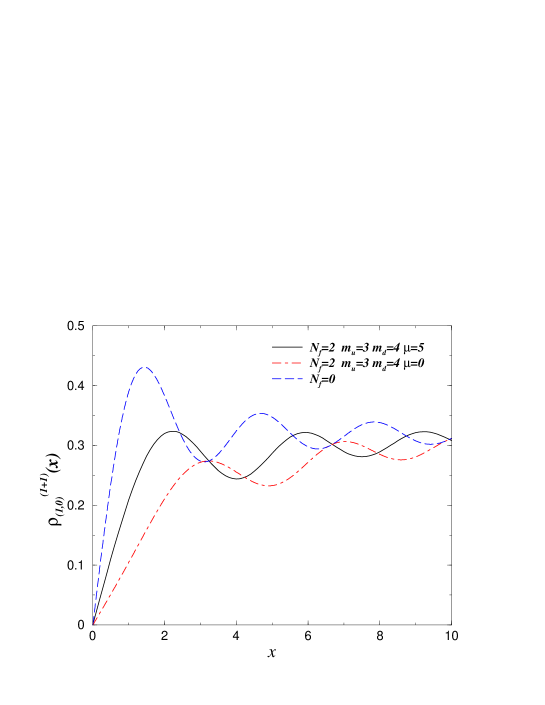
Figure 1: The eigenvalue density for $N_{f}=2$ with imaginary isospin chemical potential $\hat{\mu}=\hat{\delta}/2=0$ and $5$ and quark masses $\hat{m}_{u}=3$, $\hat{m}_{d}=4$. The quenched density eq. (3.25) of the one-matrix theory ($N_{f}=0$) is given for comparison.

To finish this subsection we give the result for the most general correlation function in the two flavor case. If follows by inserting the above building blocks into eq. (2.40) and taking out common factors:

$$\rho_{(n,k)}^{(1+1)}(\{\hat{x}\}_{n},\{\hat{y}\}_{k}) = \prod_{i=1}^{n}\hat{x}_{i}\prod_{j=1}^{k}\hat{y}_{j}\left({\cal I}^{+}(i\hat{m}_{u},i\hat{m}_{d})\right)^{-n-k}$$ (3.65)

$$\times \det_{\stackrel{{\scriptstyle 1\leq i_{1},i_{2}\leq n}}{{\ 1\leq j_{1},j_{2}\leq k}}}\left[\begin{array}[]{cc}{\cal I}^{+}(i\hat{m}_{u},i\hat{m}_{d}){\cal I}^{0}(\hat{x}_{i_{1}},\hat{x}_{i_{2}})&-{\cal I}^{+}(i\hat{m}_{u},i\hat{m}_{d})\tilde{{\cal I}}^{-}(\hat{y}_{j_{1}},\hat{x}_{i_{2}})\\ -{\cal I}^{0}(\hat{x}_{i_{1}},i\hat{m}_{u}){\cal I}^{+}(\hat{x}_{i_{2}},i\hat{m}_{d})&-{\cal I}^{0}(\hat{y}_{j_{1}},i\hat{m}_{d}){\cal I}^{0}(\hat{x}_{i_{2}},i\hat{m}_{u})\\ \\ {\cal I}^{+}(i\hat{m}_{u},i\hat{m}_{d}){\cal I}^{+}(\hat{y}_{j_{1}},\hat{x}_{i_{2}})&{\cal I}^{+}(i\hat{m}_{u},i\hat{m}_{d}){\cal I}^{0}(\hat{y}_{j_{1}},\hat{y}_{j_{2}})\\ -{\cal I}^{+}(\hat{y}_{j_{1}},i\hat{m}_{u}){\cal I}^{+}(\hat{x}_{i_{2}},i\hat{m}_{d})&-{\cal I}^{+}(\hat{y}_{j_{1}},i\hat{m}_{u}){\cal I}^{0}(\hat{y}_{j_{2}},i\hat{m}_{d})\end{array}\right]~{}.$$ (3.71)

3.3 Partial quenching

Here we consider a variant of the general $N_{f}$-theory of practical importance. We introduce $N_{f}$ fermions with Dirac operator $D_{1}$ and set $\mu_{1}=0$ then seek the spectral correlation functions between eigenvalues of $D_{1}$ and $D_{2}$ for $\mu_{2}\neq 0$. In lattice gauge theory simulations this is a simple modification. The ensemble averages are then taken with respect to a theory which is not coupled to a chemical potential, but the observables (expressed in terms of “valence quarks”) are. In the Random Matrix Theory formulation it can also be introduced straightforwardly.

The corresponding Random Matrix Theory is based on the partition function eq. (2.8) with $N_{1}=N_{f}$ and $N_{2}=0$ and we ask for the mixed correlation function $R_{(1,1)}^{(N_{f})}$ between two valence quarks associated with matrices ${\cal D}_{1,2}$. For simplicity we here restrict ourselves to the physically most interesting case of $N_{f}=2$. Here we have two sea quarks with masses $m_{u}$ and $m_{d}$ and zero chemical potential $\mu_{1}=0$, while the valence quarks have $\mu_{1}=0$ and $\mu_{2}=\delta$.

In the previous subsection the results for the most general $N_{f}=N_{1}+N_{2}$ flavors content have been given already for the polynomials in eq. (3.34) and the kernel in eq. (3.37) from which we can also compute the transforms (2.34), (2.36), (2.37) and (2.38). We just have to specify our case $N_{1}=2$, $N_{2}=0$ when applying eq. (C.8). We will first focus on $\rho_{(1,1)}^{(2)\,conn}(\hat{x},\hat{y})$ in order to pinpoint the difference between the $1+1$ flavor case eq. (3.2) from the previous subsection, which was also computed in an effective field theory approach [2]. Next, we give the general $(n,k)$-correlation function for this particular flavor combination.

The first building block for that from eq. (3.37) is given by

$$K_{N+1}^{(2)}(y,x)=\frac{h_{N}}{h_{N}^{(N_{f})}(x^{2}+m_{u}^{2})(x^{2}+m_{d}^{2})}\frac{\det\left[\begin{array}[]{ccc}K_{N+1}(y,im_{u})&P_{N+1}(-m_{u}^{2})&P_{N+2}(-m_{u}^{2})\\ K_{N+1}(y,im_{d})&P_{N+1}(-m_{d}^{2})&P_{N+2}(-m_{d}^{2})\\ K_{N+1}(y,x)&P_{N+1}(x^{2})&P_{N+2}(x^{2})\\ \end{array}\right]}{\det\left[\begin{array}[]{cc}P_{N}(-m_{u}^{2})&P_{N+1}(-m_{u}^{2})\\ P_{N}(-m_{d}^{2})&P_{N+1}(-m_{d}^{2})\\ \end{array}\right]}~{}.~{}$$ (3.72)

We observe a different structure of determinants compared to the corresponding previous result eq. (3.44), marking the difference of partial quenching. The microscopic large-$N$ limit is now easily taken using the formulas from the previous subsection. The only difference is that we have to Taylor expand the last columns in numerator and denominator as they become degenerate at large-$N$. The expansion in $1/N$ maps into a Taylor expansion with respect to the arguments and we obtain

$$\lim_{N\to\infty}K_{N+1}^{(2)}(y,x)=\frac{(2N)^{2\nu+8}(\hat{x}\hat{y})^{-\nu}\hat{\delta}^{-2}}{(\hat{x}^{2}+\hat{m}_{u}^{2})(\hat{x}^{2}+\hat{m}_{d}^{2})}\frac{\det\left[\begin{array}[]{ccc}\mathcal{I}^{+}(\hat{y},i\hat{m}_{u})&J_{\nu}(i\hat{m}_{u})&i\hat{m}_{u}J_{\nu+1}(i\hat{m}_{u})\\ \mathcal{I}^{+}(\hat{y},i\hat{m}_{d})&J_{\nu}(i\hat{m}_{d})&i\hat{m}_{d}J_{\nu+1}(i\hat{m}_{d})\\ \mathcal{I}^{+}(\hat{y},\hat{x})&J_{\nu}(\hat{x})&\hat{x}J_{\nu+1}(\hat{x})\end{array}\right]}{\det\left[\begin{array}[]{cc}J_{\nu}(i\hat{m}_{u})&i\hat{m}_{u}J_{\nu+1}(i\hat{m}_{u})\\ J_{\nu}(i\hat{m}_{d})&i\hat{m}_{d}J_{\nu+1}(i\hat{m}_{d})\end{array}\right]}~{}.$$ (3.73)

The result for the second building block of our correlation function is obtained by integrating eq. (3.72) using the definition eq. (2.38)

$$M_{N+1}^{(2)}(x,y)=\frac{h_{N}}{h_{N}^{(N_{f})}}(x^{2}+m_{u}^{2})(x^{2}+m_{d}^{2})\frac{\det\left[\begin{array}[]{ccc}H_{N+1}(x,im_{u})&P_{N+1}(-m_{u}^{2})&P_{N+2}(-m_{u}^{2})\\ H_{N+1}(x,im_{d})&P_{N+1}(-m_{d}^{2})&P_{N+2}(-m_{d}^{2})\\ M_{N+1}(x,y)&\chi_{N+1}(y)&\chi_{N+2}(y)\end{array}\right]}{\det\left[\begin{array}[]{cc}P_{N}(-m_{u}^{2})&P_{N+1}(-m_{u}^{2})\\ P_{N}(-m_{d}^{2})&P_{N+1}(-m_{d}^{2})\end{array}\right]}~{}.$$ (3.74)

In addition to the asymptotics already computed we also now need one of the transforms $\chi_{N}$. Being proportional to the polynomials, eq. (B.4), this is an easy task, and we obtain an explicit exponential $\hat{\delta}$ dependence from the prefactors. We thus arrive at

$$\lim_{N\to\infty}M_{N+1}^{(2)}(x,y)=\frac{(\hat{x}\hat{y})^{\nu+1}(\hat{x}^{2}+\hat{m}_{u}^{2})(\hat{x}^{2}+\hat{m}_{d}^{2})}{(2N)^{2\nu+6}\hat{\delta}^{2}}\frac{\det\left[\begin{array}[]{ccc}\mathcal{I}^{0}(\hat{x},i\hat{m}_{u})&J_{\nu}(i\hat{m}_{u})&i\hat{m}_{u}J_{\nu+1}(i\hat{m}_{u})\\ \mathcal{I}^{0}(\hat{x},i\hat{m}_{d})&J_{\nu}(i\hat{m}_{d})&i\hat{m}_{d}J_{\nu+1}(i\hat{m}_{d})\\ \mathcal{I}^{-}(\hat{x},\hat{y})&e^{-\hat{\delta}^{2}/2}J_{\nu}(\hat{y})&e^{-\hat{\delta}^{2}/2}G_{\nu}(\hat{y},\hat{\delta})\end{array}\right]}{\det\left[\begin{array}[]{cc}J_{\nu}(i\hat{m}_{u})&i\hat{m}_{u}J_{\nu+1}(i\hat{m}_{u})\\ J_{\nu}(i\hat{m}_{d})&i\hat{m}_{d}J_{\nu+1}(i\hat{m}_{d})\end{array}\right]}~{},$$ (3.75)

where we have introduced the notation

$$G_{\nu}(\hat{y},\hat{\delta})=\hat{y}J_{\nu+1}(\hat{y})+\hat{\delta}^{2}J_{\nu}(\hat{y})~{}.$$ (3.76)

Together with the asymptotic of the weight function,

$$\lim_{N\to\infty}w^{(2)}(x,y)~{}=~{}\frac{(\hat{x}^{2}+\hat{m}_{u}^{2})(\hat{x}^{2}+\hat{m}_{d}^{2})}{(2N)^{4}}\ \frac{(\hat{x}\hat{y})^{\nu+1}}{(2N)^{2\nu+2}}I_{\nu}\left(\frac{\hat{x}\hat{y}}{\hat{\delta}^{2}}\right)e^{-\frac{\hat{x}^{2}+\hat{y}^{2}}{2\hat{\delta}^{2}}}$$ (3.77)

we obtain the partially quenched two point function

$$\rho_{(1,1)}^{(2)\,conn}(\hat{x},\hat{y})=\hat{x}\hat{y}\ \frac{\left|\begin{array}[]{ccc}\mathcal{I}^{+}(\hat{y},i\hat{m}_{u})&J_{\nu}(i\hat{m}_{u})&i\hat{m}_{u}J_{\nu+1}(i\hat{m}_{u})\\ \mathcal{I}^{+}(\hat{y},i\hat{m}_{d})&J_{\nu}(i\hat{m}_{d})&i\hat{m}_{d}J_{\nu+1}(i\hat{m}_{d})\\ \mathcal{I}^{+}(\hat{y},\hat{x})&J_{\nu}(\hat{x})&\hat{x}J_{\nu+1}(\hat{x})\end{array}\right|\left|\begin{array}[]{ccc}-\mathcal{I}^{0}(\hat{x},i\hat{m}_{u})&J_{\nu}(i\hat{m}_{u})&i\hat{m}_{u}J_{\nu+1}(i\hat{m}_{u})\\ -\mathcal{I}^{0}(\hat{x},i\hat{m}_{d})&J_{\nu}(i\hat{m}_{d})&i\hat{m}_{d}J_{\nu+1}(i\hat{m}_{d})\\ \tilde{\mathcal{I}}^{-}(\hat{x},\hat{y})&e^{-\hat{\delta}^{2}/2}J_{\nu}(\hat{y})&e^{-\hat{\delta}^{2}/2}G_{\nu}(\hat{y},\hat{\delta})\end{array}\right|}{\left|\begin{array}[]{cc}J_{\nu}(i\hat{m}_{u})&i\hat{m}_{u}J_{\nu+1}(i\hat{m}_{u})\\ J_{\nu}(i\hat{m}_{d})&i\hat{m}_{d}J_{\nu+1}(i\hat{m}_{d})\end{array}\right|^{2}}~{}.$$ (3.78)

We note that this result is of the structure expected from the replica limit of the Toda lattice equation [21].

It is ideally suited for extracting $F_{\pi}$ from lattice simulations. To visualize the effect of partially quenching we compare the partially quenched two point function to that for $N_{f}=2$ in figure 2.

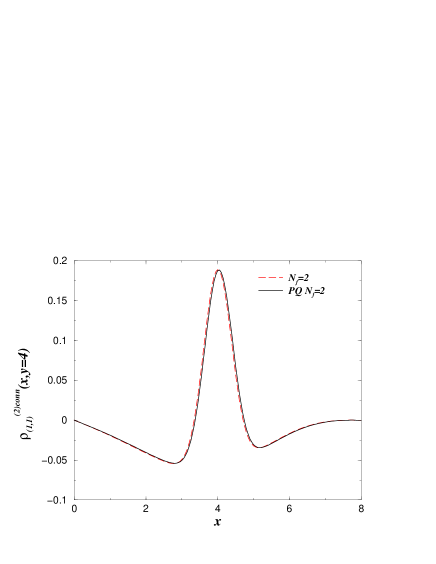
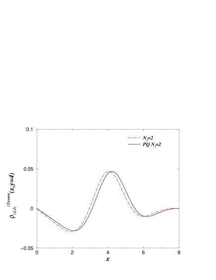
Figure 2:     The partially quenched two point function (3.78)    compared to the unquenched two point function (3.2). Here    plotted as a    function of the $D_{1}$ eigenvalue keeping the $D_{2}$ eigenvalue fixed    at $\hat{y}=4$ and setting $\hat{m}_{u}=3$ and $\hat{m}_{d}=5$. The left hand figure is for $\hat{\delta}=0.4$ and the    right hand figure is for $\hat{\delta}=1.0$. Notice the change of scale on    the vertical axis.

When the two masses are identical $m_{u}=m_{d}=m$ the expression for the partially quenched two point function becomes

$$\rho_{(1,1)}^{(2)\,conn}(\hat{x},\hat{y})=\hat{x}\hat{y}\ \frac{\left|\begin{array}[]{ccc}\mathcal{I}^{+}(\hat{y},i\hat{m})&J_{\nu}(i\hat{m})&i\hat{m}J_{\nu+1}(i\hat{m})\\ \mathcal{I}^{+}(\hat{y},i\hat{m})^{\prime}&J_{\nu}(i\hat{m})^{\prime}&(i\hat{m}J_{\nu+1}(i\hat{m}))^{\prime}\\ \mathcal{I}^{+}(\hat{y},\hat{x})&J_{\nu}(\hat{x})&\hat{x}J_{\nu+1}(\hat{x})\end{array}\right|\left|\begin{array}[]{ccc}-\mathcal{I}^{0}(\hat{x},i\hat{m})&J_{\nu}(i\hat{m})&i\hat{m}J_{\nu+1}(i\hat{m})\\ -\mathcal{I}^{0}(\hat{x},i\hat{m})^{\prime}&J_{\nu}(i\hat{m})^{\prime}&(i\hat{m}J_{\nu+1}(i\hat{m}))^{\prime}\\ \tilde{\mathcal{I}}^{-}(\hat{x},\hat{y})&e^{-\hat{\delta}^{2}/2}J_{\nu}(\hat{y})&e^{-\hat{\delta}^{2}/2}G_{\nu}(\hat{y},\hat{\delta})\end{array}\right|}{\left|\begin{array}[]{cc}J_{\nu}(i\hat{m})&i\hat{m}J_{\nu+1}(i\hat{m})\\ J_{\nu-1}(i\hat{m})&i\hat{m}J_{\nu}(i\hat{m})\end{array}\right|^{2}}~{},$$ (3.79)

where the prime indicates the derivative with respect to $i\hat{m}$.

The two remaining building blocks are given as follows. From the definition (2.36) we have from eq. (3.72)

$$H_{N+1}^{(2)}(x_{1},x_{2}) = \frac{h_{N+1}(x_{1}^{2}+m_{u}^{2})(x_{1}^{2}+m_{d}^{2})}{h_{N}^{(N_{f})}(x_{2}^{2}+m_{u}^{2})(x_{2}^{2}+m_{d}^{2})}\frac{\det\left[\begin{array}[]{ccc}H_{N+1}(x_{1},im_{u})&P_{N+1}(-m_{u}^{2})&P_{N+2}(-m_{u}^{2})\\ H_{N+1}(x_{1},im_{d})&P_{N+1}(-m_{d}^{2})&P_{N+2}(-m_{d}^{2})\\ H_{N+1}(x_{1},x_{2})&P_{N+1}(x_{2}^{2})&P_{N+2}(x_{2}^{2})\\ \end{array}\right]}{\det\left[\begin{array}[]{cc}P_{N}(-m_{u}^{2})&P_{N+1}(-m_{u}^{2})\\ P_{N}(-m_{d}^{2})&P_{N+1}(-m_{d}^{2})\\ \end{array}\right]}.$$ (3.85)

The microscopic limit is readily obtained:

$$\lim_{N\to\infty}H_{N+1}^{(2)}(x_{1},x_{2})=\frac{2N\hat{x}_{1}^{\nu+1}(\hat{x}_{1}^{2}+\hat{m}_{u}^{2})(\hat{x}_{1}^{2}+\hat{m}_{d}^{2})}{\hat{x}_{2}^{\nu}(\hat{x}_{2}^{2}+\hat{m}_{u}^{2})(\hat{x}_{2}^{2}+\hat{m}_{d}^{2})}\frac{\det\left[\begin{array}[]{ccc}\mathcal{I}^{0}(\hat{x}_{1},i\hat{m}_{u})&J_{\nu}(i\hat{m}_{u})&i\hat{m}_{u}J_{\nu+1}(i\hat{m}_{u})\\ \mathcal{I}^{0}(\hat{x}_{1},i\hat{m}_{d})&J_{\nu}(i\hat{m}_{d})&i\hat{m}_{d}J_{\nu+1}(i\hat{m}_{d})\\ \mathcal{I}^{0}(\hat{x}_{1},\hat{x}_{2})&J_{\nu}(\hat{x}_{2})&\hat{x}_{2}J_{\nu+1}(\hat{x}_{2})\end{array}\right]}{\det\left[\begin{array}[]{cc}J_{\nu}(i\hat{m}_{u})&i\hat{m}_{u}J_{\nu+1}(i\hat{m}_{u})\\ J_{\nu}(i\hat{m}_{d})&i\hat{m}_{d}J_{\nu+1}(i\hat{m}_{d})\\ \end{array}\right]}.$$ (3.87)

We note that it is $\hat{\mu}_{f}$-independent. From eq. (3.72) and the definition (2.37) we have

$$\hat{H}_{N+1}^{(2)}(y_{1},y_{2}) = \frac{h_{N+1}}{h_{N}^{(N_{f})}}\frac{\det\left[\begin{array}[]{ccc}K_{N+1}(y_{1},im_{u})&P_{N+1}(-m_{u}^{2})&P_{N+2}(-m_{u}^{2})\\ K_{N+1}(y_{1},im_{d})&P_{N+1}(-m_{d}^{2})&P_{N+2}(-m_{d}^{2})\\ \hat{H}_{N+1}(y_{1},y_{2})&\chi_{N+1}(y_{2}^{2})&\chi_{N+2}(y_{2}^{2})\\ \end{array}\right]}{\det\left[\begin{array}[]{cc}P_{N}(-m_{u}^{2})&P_{N+1}(-m_{u}^{2})\\ P_{N}(-m_{d}^{2})&P_{N+1}(-m_{d}^{2})\\ \end{array}\right]},$$ (3.93)

leading to

$$\lim_{N\to\infty}\hat{H}_{N+1}^{(2)}(y_{1},y_{2})=2N\frac{\hat{y}_{2}^{\nu+1}}{\hat{y}_{1}^{\nu}}\frac{\det\left[\begin{array}[]{ccc}\mathcal{I}^{+}(\hat{y}_{1},i\hat{m}_{u})&J_{\nu}(i\hat{m}_{u})&i\hat{m}_{u}J_{\nu+1}(i\hat{m}_{u})\\ \mathcal{I}^{+}(\hat{y}_{1},i\hat{m}_{d})&J_{\nu}(i\hat{m}_{d})&i\hat{m}_{d}J_{\nu+1}(i\hat{m}_{d})\\ \mathcal{I}^{0}(\hat{y}_{1},\hat{y}_{2})&e^{-\hat{\delta}^{2}/2}J_{\nu}(\hat{y}_{2})&e^{-\hat{\delta}^{2}/2}G_{\nu}(\hat{y}_{2},\hat{\delta}))\end{array}\right]}{\det\left[\begin{array}[]{cc}J_{\nu}(i\hat{m}_{u})&i\hat{m}_{u}J_{\nu+1}(i\hat{m}_{u})\\ J_{\nu}(i\hat{m}_{d})&i\hat{m}_{d}J_{\nu+1}(i\hat{m}_{d})\end{array}\right]}.$$ (3.94)

The two densities are given by

$$\rho_{(1,0)}^{(2)}(\hat{x}) = \lim_{N\to\infty}\frac{1}{2N}H_{N+1}^{(2)}(x,x)$$ (3.95)

$$\rho_{(0,1)}^{(2)}(\hat{y}) = \lim_{N\to\infty}\frac{1}{2N}\hat{H}_{N+1}^{(2)}(y,y)\ .$$ (3.96)

They differ because of the asymmetric flavor content, the $\hat{x}$ eigenvalues not coupling to $\hat{\mu}_{2}$. Eq. (3.95) agrees with the known result [9], as well as eq. (3.96) when setting $\hat{\mu}_{2}=0$.

We are now ready to state the most general correlation function for $N_{1}=2$ and $N_{2}=0$ flavors. Upon using the above results, taking out common factors of the determinant we obtain in terms of the abbreviations eq. (3.20)

$$\rho_{(n,k)}^{(2)}(\{\hat{x}\}_{n},\{\hat{y}\}_{k})~{}=~{}\prod_{i=1}^{n}\hat{x}_{i}\prod_{j=1}^{k}\hat{y}_{j}\det\left[\begin{array}[]{cc}J_{\nu}(i\hat{m}_{u})&i\hat{m}_{u}J_{\nu+1}(i\hat{m}_{u})\\ J_{\nu}(i\hat{m}_{d})&i\hat{m}_{d}J_{\nu+1}(i\hat{m}_{d})\end{array}\right]^{-n-k}$$ (3.99)

$$\times \left|\begin{array}[]{cc}\left|\begin{array}[]{ccc}{\cal I}^{0}(\hat{x}_{i_{1}},i\hat{m}_{u})&J_{\nu}(i\hat{m}_{u})&i\hat{m}_{u}J_{\nu+1}(i\hat{m}_{u})\\ {\cal I}^{0}(\hat{x}_{i_{1}},i\hat{m}_{d})&J_{\nu}(i\hat{m}_{d})&i\hat{m}_{d}J_{\nu+1}(i\hat{m}_{d})\\ {\cal I}^{0}(\hat{x}_{i_{1}},\hat{x}_{i_{2}})&J_{\nu}(\hat{x}_{i_{2}})&\hat{x}_{i_{2}}J_{\nu+1}(\hat{x}_{i_{2}})\end{array}\right|&\left|\begin{array}[]{ccc}{\cal I}^{0}(\hat{x}_{i_{1}},i\hat{m}_{u})&J_{\nu}(i\hat{m}_{u})&i\hat{m}_{u}J_{\nu+1}(i\hat{m}_{u})\\ {\cal I}^{0}(\hat{x}_{i_{1}},i\hat{m}_{d})&J_{\nu}(i\hat{m}_{d})&i\hat{m}_{d}J_{\nu+1}(i\hat{m}_{d})\\ -\tilde{\cal I}^{-}(\hat{x}_{i_{1}},\hat{y}_{j_{2}})&e^{-\hat{\delta}^{2}/2}J_{\nu}(\hat{y}_{j_{2}})&e^{-\hat{\delta}^{2}/2}G_{\nu}(\hat{y}_{j_{2}},\hat{\delta})\end{array}\right|\\ \\ \left|\begin{array}[]{ccc}{\cal I}^{+}(\hat{y}_{j_{1}},i\hat{m}_{u})&J_{\nu}(i\hat{m}_{u})&i\hat{m}_{u}J_{\nu+1}(i\hat{m}_{u})\\ {\cal I}^{+}(\hat{y}_{j_{1}},i\hat{m}_{d})&J_{\nu}(i\hat{m}_{d})&i\hat{m}_{d}J_{\nu+1}(i\hat{m}_{d})\\ {\cal I}^{+}(\hat{y}_{j_{1}},\hat{x}_{i_{2}})&J_{\nu}(\hat{x}_{i_{2}})&\hat{x}_{i_{2}}J_{\nu+1}(\hat{x}_{i_{2}})\end{array}\right|&\left|\begin{array}[]{ccc}{\cal I}^{+}(\hat{y}_{j_{1}},i\hat{m}_{u})&J_{\nu}(i\hat{m}_{u})&i\hat{m}_{u}J_{\nu+1}(i\hat{m}_{u})\\ {\cal I}^{+}(\hat{y}_{j_{1}},i\hat{m}_{d})&J_{\nu}(i\hat{m}_{d})&i\hat{m}_{d}J_{\nu+1}(i\hat{m}_{d})\\ {\cal I}^{0}(\hat{y}_{j_{1}},\hat{y}_{j_{2}})&e^{-\hat{\delta}^{2}/2}J_{\nu}(\hat{y}_{j_{2}})&e^{-\hat{\delta}^{2}/2}G_{\nu}(\hat{y}_{j_{2}},\hat{\delta})\end{array}\right|\end{array}\right|.$$ (3.115)

As expected we verify that all correlation functions of eigenvalues $\hat{x}_{j}$ are $\hat{\mu}$-independent and agree with the results of [9].

4 The non-chiral Two-Matrix Problem

Having discussed the chiral Unitary Two-Matrix Theory in great detail it is a small step to go through the same analysis in the ordinary Unitary Two-Matrix Theory. As mentioned briefly in the introduction, this ensemble is relevant for QCD in three space-time dimensions, and may have applications in condensed matter physics as well [16].

It is straightforward to consider two arbitrary chemical potentials $\mu_{1}$ and $\mu_{2}$, as in the chiral case treated above. However, for simplicity we restrict ourselves to just imaginary isospin chemical potential, $i.e.$ the case where $\mu_{1}=-\mu_{2}\equiv\mu$. We present the most general case with an even number of flavors, $2N_{f}=2N_{+}+2N_{-}$. The techniques used here can also be applied to the case of an odd number of flavors. The masses are pairwise equal in magnitude but of opposite sign [14, 15]

$$m_{+1},\ldots,m_{+N_{+}},-m_{+1},\ldots,-m_{+N_{+}},\ \ \mbox{and}\ \ m_{-1},\ldots,m_{-N_{-}},-m_{-1},\ldots,-m_{-N_{-}}.$$ (4.1)

Both positive and negative mass fermions are coupled to imaginary isospin potential. In intermediate steps also an odd number of flavors will appear. The Dirac operator then remains anti-hermitian as in four dimensions, and the corresponding Random Two-Matrix Theory reads

$${\cal Z}^{(2N_{f})}(\{m_{+}\},\{m_{-}\})\sim\int\!d\Phi d\Psi\exp\left[-{N}{\rm Tr}\left(\Phi^{2}+\Psi^{2}\right)\right]\prod_{f=1}^{2N_{+}}\det[{\cal D_{+}}(\mu)+m_{+f}]\!\prod_{g=1}^{2N_{-}}\det[{\cal D_{-}}(\mu)+m_{-g}],$$ (4.2)

where both $\Phi$ and $\Psi$ now are $N\times N$ hermitian matrices, and

$${\cal D}_{\pm}(\mu)~{}\equiv~{}i\Phi\pm i\mu\Psi~{}\equiv~{}i\Phi_{\pm}~{}.$$ (4.3)

A related non-hermitian matrix model aimed at real baryon chemical potential was considered in ref. [32]. Here we again restrict ourselves to the Gaussian case for convenience. The same remarks we made about non-Gaussian potentials from the previous section also apply here. For the Riemann-Hilbert problem to be solved in order to prove universality in the quenched case we refer to [33].

We next perform the same change of variables as in eq. (2.6) to obtain

$${\cal Z}^{(2N_{f})}(\{m_{+}\},\{m_{-}\})\sim\int\!\!d\Phi_{+}d\Phi_{-}\!\prod_{f=1}^{2N_{+}}\det[i\Phi_{+}+m_{+f}]\prod_{g=1}^{2N_{-}}\det[i\Phi_{-}+m_{-g}]\exp\!\left[-\frac{N}{4}{\rm Tr}V(\Phi_{+},\Phi_{-})\right],$$ (4.4)

with a potential

$$V(\Phi_{+},\Phi_{-})~{}=~{}\frac{\mu^{2}+1}{\mu^{2}}\left(\Phi_{+}^{2}+\Phi_{-}^{2}\right)+2\frac{\mu^{2}-1}{\mu^{2}}\Phi_{+}\Phi_{-}~{}.$$ (4.5)

Going to an eigenvalue representation can be done exactly as in refs. [25, 26]. Because of the pairing in positive and negative masses the integration measure takes the following form

$${\cal Z}^{(2N_{f})}(\{m_{+}\},\{m_{-}\}) = \int_{-\infty}^{\infty}\prod_{i=1}^{N}\left(dx_{i}dy_{i}\prod_{f=1}^{N_{+}}(x_{i}^{2}+m_{+f}^{2})\prod_{g=1}^{N_{-}}(y_{i}^{2}+m_{-g}^{2})\right)$$ (4.7)

$$\times\Delta_{N}(\{x\})\Delta_{N}(\{y\})\det\left[\exp\left(N\frac{1-\mu^{2}}{2\mu^{2}}x_{i}y_{j}\right)\right]e^{-N\frac{\mu^{2}+1}{4\mu^{2}}\sum_{i}^{N}(x_{i}^{2}+y_{i}^{2})}~{}.$$

Due to the presence of determinant factors in the measure this is a generalization of the ordinary (quenched) Gaussian Unitary Random Two-Matrix Model considered in the literature [25, 26, 13, 29]. We seek biorthogonal polynomials satisfying

$$\int_{-\infty}^{\infty}dxdy\ w^{(2N_{f})}(x,y)\ P_{n}^{(2N_{f})}(x)\ Q_{k}^{(2N_{f})}(y)=h_{n}^{(2N_{f})}\delta_{nk}~{},$$ (4.8)

with respect to the weight function

$$w^{(2N_{f})}(x,y)~{}\equiv~{}\prod_{f=1}^{N_{+}}(x^{2}+m_{+f}^{2})\prod_{g=1}^{N_{-}}(y^{2}+{m}_{-g}^{2})\ e^{N\frac{1-\mu^{2}}{2\mu^{2}}xy}e^{-N\frac{\mu^{2}+1}{4\mu^{2}}(x^{2}+y^{2})}\ .$$ (4.9)

The only difference to the previous section is that the $I$-Bessel function is replaced by an exponential and that we integrate over the full real line. Our polynomials are now polynomials in $x$ and $y$, and not in their squares. Furthermore all factors $(x^{2}+m_{f}^{2})$ are counted as two flavors with masses $\pm im_{f}$, instead of one in the previous section.

Taking into account these differences all definitions of the transforms eq. (2.34) and the four kernels eqs. (2.35) - (2.38) carry trough and we shall not repeat them here. The eigenvalue correlation functions defined as

$$R_{(n,k)}^{(2N_{f})}(\{x\}_{n},\{y\}_{k}) \equiv \frac{N!^{2}}{(N-n)!(N-k)!}\frac{1}{{\cal Z}^{(2N_{f})}(\{m_{+}\},\{m_{-}\})}\int_{-\infty}^{\infty}\prod_{j=n+1}^{N}dx_{j}\prod_{l=k+1}^{N}dy_{l}\det\left[e^{N\frac{1-\mu^{2}}{2\mu^{2}}x_{i}y_{j}}\right]$$ (4.10)

$$\times \prod_{i=1}^{N}\left(\prod_{f=1}^{N_{+}}(x_{i}^{2}+m_{+f}^{2})\prod_{g=1}^{N_{-}}(y_{i}^{2}+m_{-g}^{2})\right)e^{-N\frac{\mu^{2}+1}{4\mu^{2}}\sum_{i}^{N}(x_{i}^{2}+y_{i}^{2})}\Delta_{N}(\{x\})\Delta_{N}(\{y\})\ .$$ (4.11)

are given by the same formula eq. (2.40) in terms of the corresponding non-chiral kernels.

4.1 The quenched case

The quenched case corresponds to omitting the explicit factors of determinants from the measure, while still performing the change of variables (4.3). We then get the standard Random Two-Matrix Model, with a coupling between the two matrices $\Phi_{\pm}$ as given by eq. (4.5). We will need these results later when expressing the unquenched results in terms of the quenched ones.

The biorthogonality condition (4.8) becomes

$$\int_{-\infty}^{\infty}dxdy\ e^{N\frac{1-\mu^{2}}{2\mu^{2}}xy}e^{-N\frac{\mu^{2}+1}{4\mu^{2}}(x^{2}+y^{2})}P_{n}(x)P_{m}(y)~{}=~{}h_{n}\delta_{nm}~{}.$$ (4.13)

Because of the weight being symmetric in $x$ and $y$ we have that $Q_{n}(y)=P_{n}(y)$. It was noted indirectly in refs. [34] and [28] that this condition is related to Hermite polynomials, although precise details were not given there. This can also be seen along the same lines as in appendix A. In our conventions we find for the monic polynomials

$$P_{n}(x)~{}=~{}2^{-n}\left(\frac{\mu^{2}+1}{N}\right)^{\frac{n}{2}}H_{n}\left(\sqrt{\frac{N}{\mu^{2}+1}}\ x\right).$$ (4.14)

For the normalization constants we obtain

$$h_{n}~{}=~{}\frac{\mu\pi}{2^{n-1}N^{n+1}}\ n!\ (1-\mu^{2})^{n}\ .$$ (4.15)

The factorization of the weight observed in Appendix B also applies here. The weight $w(x,y)$ is given by the sum over the biorthogonal polynomials

$$w(x,y) = \exp\left[-N\frac{\mu^{2}+1}{4\mu^{2}}(x^{2}+y^{2})+N\frac{1-\mu^{2}}{2\mu^{2}}xy\right]$$

$$= \frac{2\mu}{1+\mu^{2}}e^{-\frac{N}{\mu^{2}+1}(x^{2}+y^{2})}\sum_{k=0}^{\infty}\frac{1}{k!}\left(\frac{1-\mu^{2}}{2(\mu^{2}+1)}\right)^{k}H_{k}\left(\sqrt{\frac{N}{\mu^{2}+1}}\ x\right)H_{k}\left(\sqrt{\frac{N}{\mu^{2}+1}}\ y\right),$$

using the Mehler formula for Hermite polynomials. The individual factors are obviously $w_{1}(x)=w_{2}(x)=e^{-\frac{N}{\mu^{2}+1}x^{2}}$.

The functions $\chi_{n}(x)$ can be found explicitly by integrating the polynomials. Alternatively, we could also use the results from the previous section by setting $\nu=\pm\frac{1}{2}$ and using the relation (4.23) below. The $I$-Bessel function then becomes a hyperbolic sine or cosine and the two terms add up to an integral over the full real line. The result is

$$\chi_{n}(x)~{}=~{}\frac{\mu\sqrt{\pi}}{2^{n-1}N^{\frac{n+1}{2}}}\frac{(1-\mu^{2})^{n}}{(\mu^{2}+1)^{\frac{n+1}{2}}}\ e^{-\frac{N}{\mu^{2}+1}x^{2}}H_{n}\left(\sqrt{\frac{N}{\mu^{2}+1}}\ x\right)\ ,$$ (4.17)

again being proportional to the polynomials. The three different quenched kernels thus read as follows:

$$K_{N}(y,x) = \sum_{k=0}^{N-1}\frac{N}{\pi\mu\ k!\ 2^{k+1}}\frac{(\mu^{2}+1)^{k}}{(1-\mu^{2})^{k}}H_{k}\left(\sqrt{\frac{N}{\mu^{2}+1}}\ x\right)H_{k}\left(\sqrt{\frac{N}{\mu^{2}+1}}\ y\right)$$ (4.18)

$$H_{N}(x,y) = \sum_{k=0}^{N-1}\frac{N^{\frac{1}{2}}}{\sqrt{\pi}\ k!\ 2^{k}}\frac{1}{(\mu^{2}+1)^{\frac{1}{2}}}H_{k}\left(\sqrt{\frac{N}{\mu^{2}+1}}\ x\right)H_{k}\left(\sqrt{\frac{N}{\mu^{2}+1}}\ y\right)\ e^{-\frac{N}{\mu^{2}+1}x^{2}}$$ (4.19)

$$= \hat{H}_{N}(y,x)$$ (4.20)

$$M_{N}(x,y) = \sum_{k=0}^{N-1}\frac{\mu}{k!\ 2^{k-1}}\frac{(1-\mu^{2})^{k}}{(\mu^{2}+1)^{k+1}}H_{k}\left(\sqrt{\frac{N}{\mu^{2}+1}}\ x\right)H_{k}\left(\sqrt{\frac{N}{\mu^{2}+1}}\ y\right)e^{-\frac{N}{\mu^{2}+1}(x^{2}+y^{2})}.$$ (4.21)

With this result we can now obtain all spectral correlation functions via eq. (2.40).

To take the scaling limit, we make use of the relations between Hermite and Laguerre polynomials,

$$H_{2n}(x) = (-1)^{n}2^{2n}n!\ L_{n}^{(-1/2)}(x^{2})$$ (4.22)

$$H_{2n+1}(x) = (-1)^{n}2^{2n+1}n!\ x\,L_{n}^{(1/2)}(x^{2})\ ,$$ (4.23)

and the asymptotic behavior of Laguerre polynomials (3.10). This gives

$$H_{2n}(X) \to (-1)^{n}2^{2n}n!\ n^{-\frac{1}{2}}\frac{1}{\sqrt{\pi}}\cos(\sqrt{4n}\ X)$$ (4.24)

$$H_{2n+1}(X) \to (-1)^{n}2^{2n+1}n!\ \frac{1}{\sqrt{\pi}}\sin(\sqrt{4n}\ X)\ .$$ (4.25)

If we rescale $\sqrt{2}Nx=\hat{x}$, $\sqrt{2}Ny=\hat{y}$ leading to the customary level spacing $\frac{1}{\pi}$ we arrive at the following asymptotic for the kernels:

$$\lim_{N\to\infty}K_{N}\left(x=\frac{\hat{x}}{\sqrt{2}N},y=\frac{\hat{y}}{\sqrt{2}N}\right) = \frac{N^{2}}{\sqrt{\pi}\hat{\mu}}\ {\cal I}^{+}(\hat{x},\hat{y})$$ (4.26)

$$\lim_{N\to\infty}H_{N}\left(x=\frac{\hat{x}}{\sqrt{2}N},y=\frac{\hat{y}}{\sqrt{2}N}\right) = {\sqrt{2}\ N}\ {\cal I}^{0}(\hat{x},\hat{y})$$ (4.27)

$$= \lim_{N\to\infty}\hat{H}_{N}\left(y=\frac{\hat{y}}{\sqrt{2}N},x=\frac{\hat{x}}{\sqrt{2}N}\right)$$ (4.28)

$$\lim_{N\to\infty}M_{N}\left(x=\frac{\hat{x}}{\sqrt{2}N},y=\frac{\hat{y}}{\sqrt{2}N}\right) = 2\hat{\mu}\sqrt{\pi}\ {\cal I}^{-}(\hat{x},\hat{y})\ ,$$ (4.30)

where we have introcued the following notation

$${\cal I}^{\pm}(x,y) \equiv \frac{1}{\pi}\int_{0}^{1}ds\ e^{\pm\hat{\mu}^{2}s^{2}}\cos(s(x-y))$$ (4.31)

$${\cal I}^{0}(x,y) \equiv \frac{1}{\pi}\int_{0}^{1}ds\ \cos(s(x-y))\ =\ \frac{1}{\pi}\frac{\sin({x}-{y})}{({x}-{y})}\ .$$ (4.32)

The arguments can be real or imaginary. In the asymptotic we have replaced the sums by integrals and used again eq. (3.12) with $t=k/N$. For convenience we have kept the scaling $2N\mu^{2}=\hat{\mu}^{2}$ as in the previous section. The weight function has the following limit:

$$\lim_{N\to\infty}w\left(x=\frac{\hat{x}}{\sqrt{2}N},y=\frac{\hat{y}}{\sqrt{2}N}\right)~{}=~{}\exp\left(-\frac{(\hat{x}-\hat{y})^{2}}{8\hat{\mu}^{2}}\right).$$ (4.33)

We will also use the following abbreviation in this section:

$$\tilde{\cal I}^{-}(x,y)\ \equiv\ \frac{1}{2\hat{\mu}\sqrt{\pi}}\exp\left(-\frac{(x-y)^{2}}{8\hat{\mu}^{2}}\right)-\frac{1}{\pi}\int_{0}^{1}ds\ e^{-\hat{\mu}^{2}s^{2}}\cos(s(x-y))\ .$$ (4.34)

Putting all together we obtain from the definition (3.23) with $(2N)^{-n-k}$ replaced by $(\sqrt{2}N)^{-n-k}$

$$\rho_{(n,k)}(\{\hat{x}\},\{\hat{y}\})=\det\left[\begin{array}[]{cc}{\cal I}^{0}(\hat{x}_{i_{1}},\hat{x}_{i_{2}})&-\tilde{\cal I}^{-}(\hat{x}_{i_{1}},\hat{y}_{j_{2}})\\ &\\ {\cal I}^{+}(\hat{y}_{j_{1}},\hat{x}_{i_{2}})&{\cal I}^{0}(\hat{y}_{j_{1}},\hat{y}_{j_{2}})\\ \end{array}\right],$$ (4.35)

after taking out common factors from the determinant. As a check we obtain that the following densities are constant and $\hat{\mu}$-independent:

$$\rho_{(1,0)}(\hat{x})~{}=~{}\rho_{(0,1)}(\hat{x})~{}=~{}\frac{1}{\pi}\ ,$$ (4.36)

and we also recover the known correlations of the one-matrix model in terms of the sine-kernel for $\rho_{(n,0)}({\hat{x}})$ and $\rho_{(0,k)}({\hat{y}})$ respectively.

4.2 Two and more flavors

In this subsection we outline how the insertion of flavors can be reexpressed in terms of quenched quantities as in the last section, and we will also give some examples.

The biorthogonal polynomials enjoy again a determinental form as in eq. (3.31)

$$P_{k}^{(2N_{f})}(x) = (-i)^{k}\langle\det[{\mathcal{D_{+}}}(\mu)-ix]\rangle_{{\cal Z}^{(2N_{f})}}$$ (4.37)

$$= \frac{(-)^{k}}{{\cal Z}^{(2N_{f})}}\int_{-\infty}^{\infty}\prod_{j=1}^{k}\left(dx_{j}dy_{j}(x_{j}-x)\prod_{f}^{N_{+}}(x_{j}^{2}+m_{+f}^{2})\prod_{g}^{N_{-}}(y_{j}^{2}+{m}_{-g}^{2})\right)$$ (4.39)

$$\times\Delta_{k}(\{x\})\Delta_{k}(\{y\})\det\left[\exp(N\frac{1-\mu^{2}}{2\mu^{2}}x_{i}y_{j})\right]\ e^{-N\frac{\mu^{2}+1}{4\mu^{2}}\sum_{i}^{k}(x_{i}^{2}+y_{i}^{2})}\ ,$$

and similarly for

$$Q_{k}^{(2N_{f})}(y)~{}=~{}(-i)^{k}\langle\det{\mathcal{D_{-}}}(\mu)-iy\rangle_{{\cal Z}^{(2N_{f})}}\ .$$ (4.40)

The kernel of both polynomials is given by

$$K_{N+1}^{(2N_{f})}(y,x) = \frac{(-)^{k}}{h_{N}^{(2N_{f})}}\langle\det[{\mathcal{D_{+}}}(\mu)-ix]\det[{\mathcal{D_{-}}}(\mu)-iy]\rangle_{{\cal Z}^{(2N_{f})}}$$ (4.41)

$$= \frac{1}{h_{N}^{(2N_{f})}{\cal Z}^{(2N_{f})}}\int_{-\infty}^{\infty}\prod_{i}^{N}\left(dx_{i}dy_{i}(x_{i}-x)(y_{i}-y)\prod_{f}^{N_{+}}(x_{i}^{2}+m_{+f}^{2})\prod_{g}^{N_{-}}(y_{i}^{2}+{m}_{-g}^{2})\right)$$ (4.43)

$$\times\Delta_{N}(\{x\})\Delta_{N}(\{y\})\det\left[\exp(N\frac{1-\mu^{2}}{2\mu^{2}}x_{i}y_{j})\right]\ e^{-N\frac{\mu^{2}+1}{4\mu^{2}}\sum_{i}^{N}(x_{i}^{2}+y_{i}^{2})}\ ,$$

with the norms given in eq. (3.36). We recall that when applying appendix C all different masses in eq. (4.1) are counted as individual flavors, positive and negative, leading to one column or row in eq. (C.8) each. The remaining kernels can be obtained from the definitions eqs. (2.36) - (2.38). The most general correlation function then follows from eq. (2.40).

All these quantities, the transformed polynomials and the remaining kernels can be in principle be expressed in terms of partition functions. They are given by eq. (C.8): eqs. (3.34), (3.37), and by inserting the kernel, (3.37), in the definitions (2.36) - (2.38), with the obvious modification of dropping the $\nu$ terms and writing polynomials with arguments of power one. However, there is a subtlety here as the partition function in eq. (4.39) contains an odd number of flavors. There are two such partition functions available [14, 15]

$${\cal Z}_{\rm even}^{(2N_{f}+1)} = \int_{U(2N_{f}+1)}\!dU\cosh[V\Sigma{\mbox{\rm Tr}({\cal M}}U\Gamma_{5}U^{\dagger})]\ ,$$ (4.44)

$${\cal Z}_{\rm odd}^{(2N_{f}+1)} = \int_{U(2N_{f}+1)}\!dU\sinh[V\Sigma{\mbox{\rm Tr}({\cal M}}U\Gamma_{5}U^{\dagger})]\ ,$$ (4.45)

with $\Gamma_{5}=$diag(1${}_{N_{f}}$,1${}_{N_{f}+1})$, being even and odd in the masses, respectively. Consequently the even polynomials $P_{2k}$ are given by eq. (4.44) whereas the odd ones $P_{2k+1}$ are given by eq. (4.45). Similarly special care has to be taken when adding single unpaired flavors to each of the sectors $N_{+}$ and $N_{-}$ as in the kernel eq. (4.43), and we refer to [15] for the relation between partition functions of chiral and non-chiral theories at $\mu=0$. Although similar massive partition functions with chemical potential have been computed from complex matrix models [32] and effective field theory [21] we do not further pursue this route. Alternatively we can explicitly compute the large-$N$ limit from our biorthogonal polynomials and kernels, as we will show in the following example.

Let us consider the simplest case with $2N_{+}=2$ flavors of masses $\pm m$, and no other flavors: $2N_{-}=0$. The corresponding weight function reads

$$w^{(2)}(x,y)~{}=~{}(x^{2}+m^{2})\ e^{N\frac{1-\mu^{2}}{2\mu^{2}}xy}e^{-N\frac{\mu^{2}+1}{4\mu^{2}}(x^{2}+y^{2})}\ .$$ (4.46)

The kernel is almost identical to the partially quenched one eq. (3.72):

$$K_{N+1}^{(2)}(y,x)=\frac{h_{N+1}}{h_{N}^{(N_{f})}(x-im)(x+im)}\frac{\det\left[\begin{array}[]{ccc}K_{N+1}(y,im)&P_{N+1}(im)&P_{N+2}(im)\\ K_{N+1}(y,-im)&P_{N+1}(-im)&P_{N+2}(-im)\\ K_{N+1}(y,x)&P_{N+1}(x^{2})&P_{N+2}(x^{2})\\ \end{array}\right]}{\det\left[\begin{array}[]{cc}P_{N}(im)&P_{N+1}(im)\\ P_{N}(-im)&P_{N+1}(-im)\\ \end{array}\right]}.$$ (4.52)

The large-$N$ limit is easily obtained using the results of the previous subsection, rescaling the mass as the eigenvalues $\sqrt{2}Nm=\hat{m}$:

$$\lim_{N\to\infty}K_{N+1}^{(2)}(y,x) = \frac{2N^{2}}{(\hat{x}^{2}+\hat{m}^{2})}\ \frac{N^{2}}{\hat{\mu}\sqrt{\pi}}\frac{\det\left[\begin{array}[]{ccc}{\cal I}^{+}(\hat{y},i\hat{m})&\cosh(\hat{m})&-i\sinh(\hat{m})\\ {\cal I}^{+}(\hat{y},-i\hat{m})&\cosh(\hat{m})&i\sinh(\hat{m})\\ {\cal I}^{0}(\hat{y},\hat{x})&\cos(\hat{x})&-\sin(\hat{x})\\ \end{array}\right]}{\det\left[\begin{array}[]{cc}i\sinh(\hat{m})&\cosh(\hat{m})\\ -i\sinh(\hat{m})&\cosh(\hat{m})\\ \end{array}\right]}.$$ (4.58)

Here we have chosen $N$ to be even, noticing the difference between the asymptotic of $P_{N}$ and $P_{N+2}$ by a factors of $(-1)$. Odd $N$ leads to the same result, as can be seen from interchanging the last two columns in numerator and denominator. Similarly the kernel can be seen to be real as it should. The remaining kernels follow with the same modifications from eqs. (3.74), (LABEL:H2) and (3.93). Therefore we just give the results here:

$$\lim_{N\to\infty}M_{N+1}^{(2)}(x,y)=2\hat{\mu}\sqrt{\pi}\frac{(\hat{x}^{2}+\hat{m}^{2})}{2N^{2}}\frac{\det\left[\begin{array}[]{ccc}{\cal I}^{0}(\hat{y},i\hat{m})&\cosh(\hat{m})&-i\sinh(\hat{m})\\ {\cal I}^{0}(\hat{y},-i\hat{m})&\cosh(\hat{m})&i\sinh(\hat{m})\\ {\cal I}^{-}(\hat{x},\hat{y})&e^{-\hat{\mu}^{2}}\cos(\hat{y})&-e^{-\hat{\mu}^{2}}(\sin(\hat{y})+2\hat{\mu}^{2}\cos(\hat{y}))\\ \end{array}\right]}{\det\left[\begin{array}[]{cc}i\sinh(\hat{m})&\cosh(\hat{m})\\ -i\sinh(\hat{m})&\cosh(\hat{m})\\ \end{array}\right]},$$ (4.64)

$$\lim_{N\to\infty}H_{N+1}^{(2)}(x_{1},x_{2}) = \sqrt{2}\ N\frac{(\hat{x}_{1}^{2}+\hat{m}^{2})}{(\hat{x}_{2}^{2}+\hat{m}^{2})}\frac{\det\left[\begin{array}[]{ccc}{\cal I}^{0}(\hat{x}_{1},i\hat{m})&\cosh(\hat{m})&-i\sinh(\hat{m})\\ {\cal I}^{0}(\hat{x}_{1},-i\hat{m})&\cosh(\hat{m})&i\sinh(\hat{m})\\ {\cal I}^{0}(\hat{x}_{1},\hat{x}_{2})&\cos(\hat{x}_{2})&-\sin(\hat{x}_{2})\\ \end{array}\right]}{\det\left[\begin{array}[]{cc}i\sinh(\hat{m})&\cosh(\hat{m})\\ -i\sinh(\hat{m})&\cosh(\hat{m})\\ \end{array}\right]},$$ (4.71)

which is $\mu$-independent, and

$$\lim_{N\to\infty}\hat{H}_{N+1}^{(2)}(y_{1},y_{2})=\sqrt{2}\ N\frac{\det\left[\begin{array}[]{ccc}{\cal I}^{+}(\hat{y}_{1},i\hat{m})&\cosh(\hat{m})&-i\sinh(\hat{m})\\ {\cal I}^{+}(\hat{y}_{1},-i\hat{m})&\cosh(\hat{m})&i\sinh(\hat{m})\\ {\cal I}^{0}(\hat{y}_{1},\hat{y}_{2})&e^{-\hat{\mu}^{2}}\cos(\hat{y}_{2})&-e^{-\hat{\mu}^{2}}(\sin(\hat{y}_{2})+2\hat{\mu}^{2}\cos(\hat{y}_{2}))\\ \end{array}\right]}{\det\left[\begin{array}[]{cc}i\sinh(\hat{m})&\cosh(\hat{m})\\ -i\sinh(\hat{m})&\cosh(\hat{m})\\ \end{array}\right]}.$$ (4.78)

(4.79)

We can write the general correlation function as follows:

$$\rho_{(n,k)}^{(2)}(\{\hat{x}\}_{n},\{\hat{y}\}_{k})~{}=~{}\det\left[\begin{array}[]{cc}i\sinh(\hat{m})&\cosh(\hat{m})\\ -i\sinh(\hat{m})&\cosh(\hat{m})\\ \end{array}\right]^{-n-k}\times$$ (4.82)

$$\left|\begin{array}[]{cc}\left|\begin{array}[]{ccc}{\cal I}^{0}(\hat{x}_{i_{1}},i\hat{m})&\cosh(\hat{m})&-i\sinh(\hat{m})\\ {\cal I}^{0}(\hat{x}_{i_{1}},-i\hat{m})&\cosh(\hat{m})&i\sinh(\hat{m})\\ {\cal I}^{0}(\hat{x}_{i_{1}},\hat{x}_{i_{2}})&\cos(\hat{x}_{i_{2}})&-\sin(\hat{x}_{i_{2}})\\ \end{array}\right|&\left|\begin{array}[]{ccc}{\cal I}^{0}(\hat{x}_{i_{1}},i\hat{m})&\cosh(\hat{m})&-i\sinh(\hat{m})\\ {\cal I}^{0}(\hat{x}_{i_{1}},-i\hat{m})&\cosh(\hat{m})&i\sinh(\hat{m})\\ -\tilde{\cal I}^{-}(\hat{x}_{i_{1}},\hat{y}_{j_{2}})&e^{-\hat{\mu}^{2}}\cos(\hat{y}_{j_{2}})&-e^{-\hat{\mu}^{2}}(\sin(\hat{y}_{j_{2}})+2\hat{\mu}^{2}\cos(\hat{y}_{j_{2}}))\\ \end{array}\right|\\ &\\ \left|\begin{array}[]{ccc}{\cal I}^{+}(\hat{y}_{j_{1}},i\hat{m})&\cosh(\hat{m})&-i\sinh(\hat{m})\\ {\cal I}^{+}(\hat{y}_{j_{1}},-i\hat{m})&\cosh(\hat{m})&i\sinh(\hat{m})\\ {\cal I}^{+}(\hat{y}_{j_{1}},\hat{x}_{i_{2}})&\cos(\hat{x}_{i_{2}})&-\sin(\hat{x}_{i_{2}})\\ \end{array}\right|&\left|\begin{array}[]{ccc}{\cal I}^{+}(\hat{y}_{j_{1}},i\hat{m})&\cosh(\hat{m})&-i\sinh(\hat{m})\\ {\cal I}^{+}(\hat{y}_{j_{1}},-i\hat{m})&\cosh(\hat{m})&i\sinh(\hat{m})\\ {\cal I}^{0}(\hat{y}_{j_{1}},\hat{y}_{j_{2}})&e^{-\hat{\mu}^{2}}\cos(\hat{y}_{j_{2}})&-e^{-\hat{\mu}^{2}}(\sin(\hat{y}_{j_{2}})+2\hat{\mu}^{2}\cos(\hat{y}_{j_{2}}))\\ \end{array}\right|\end{array}\right|$$ (4.98)

From the density

$$\rho_{(1,0)}^{(2)}(\hat{x})=\lim_{N\to\infty}\frac{1}{\sqrt{2}N}H_{N+1}^{(2)}(x,x)$$ (4.99)

and from $\rho^{(2)}_{(0,1)}(\hat{y})$ in the limit $\hat{\mu}\to 0$ we recover the known massive density from the second of ref. [14]. Similarly all higher correlators at $\hat{\mu}=0$ can be recovered.

Our second example is for $N_{+}=N_{-}=1$ flavors with masses $m_{+}$ and $m_{-}$. The structure is very similar to the example in subsection 3.2, but with twice the flavor content: $2N_{f}=2+2$ here. The four kernels at finite-$N$ are similar to those given by eqs. (3.44), (3.48), (3.53) and (3.58), with $2\times 2$ and $3\times 3$ determinants in denominator and numerator here. For example the first kernel reads

$$K_{N+1}^{(2+2)}(y,x) = \frac{h_{N+1}}{h_{N}^{(N_{f})}(x^{2}+m_{+}^{2})(y^{2}+m_{-}^{2})}\frac{1}{\det\left[\begin{array}[]{cc}K_{N+1}(im_{-},im_{+})&K_{N+1}(im_{-},-im_{+})\\ K_{N+1}(-im_{-},im_{+})&K_{N+1}(-im_{-},-im_{+})\\ \end{array}\right]}$$ (4.106)

$$\times\det\left[\begin{array}[]{ccc}K_{N+1}(im_{-},im_{+})&K_{N+1}(im_{-},-im_{+})&K_{N+1}(im_{-},x)\\ K_{N+1}(-im_{-},im_{+})&K_{N+1}(-im_{-},-im_{+})&K_{N+1}(-im_{-},x)\\ K_{N+1}(y,im_{+})&K_{N+1}(y,-im_{+})&K_{N+1}(y,x)\\ \end{array}\right],$$

with an asymptotic limit

$$\lim_{N\to\infty}K_{N+1}^{(2+2)}(y,x) = \frac{2N^{2}}{(\hat{x}^{2}+\hat{m}_{+}^{2})(\hat{y}^{2}+\hat{m}_{-}^{2})}\frac{N^{2}}{\sqrt{\pi}\hat{\mu}}\frac{1}{\det\left[\begin{array}[]{cc}{\cal I}^{+}(i\hat{m}_{-},i\hat{m}_{+})&{\cal I}^{+}(i\hat{m}_{-},-i\hat{m}_{+})\\ {\cal I}^{+}(-i\hat{m}_{-},i\hat{m}_{+})&{\cal I}^{+}(-i\hat{m}_{-},-i\hat{m}_{+})\\ \end{array}\right]}$$ (4.113)

$$\times\det\left[\begin{array}[]{ccc}{\cal I}^{+}(i\hat{m}_{-},i\hat{m}_{+})&{\cal I}^{+}(i\hat{m}_{-},-i\hat{m}_{+})&{\cal I}^{+}(i\hat{m}_{-},\hat{x})\\ {\cal I}^{+}(-i\hat{m}_{-},i\hat{m}_{+})&{\cal I}^{+}(-i\hat{m}_{-},-i\hat{m}_{+})&{\cal I}^{+}(-i\hat{m}_{-},\hat{x})\\ {\cal I}^{+}(\hat{y},i\hat{m}_{+})&{\cal I}^{+}(\hat{y},-i\hat{m}_{+})&{\cal I}^{+}(\hat{y},\hat{x})\\ \end{array}\right].$$

The remaining kernels can be obtained similary, and we only give their asymptotic expressions:

$$\lim_{N\to\infty}M_{N+1}^{(2+2)}(x,y) = \frac{(\hat{x}^{2}+\hat{m}_{+}^{2})(\hat{y}^{2}+\hat{m}_{-}^{2})}{2N^{2}}2\sqrt{\pi}\hat{\mu}\frac{1}{\det\left[\begin{array}[]{cc}{\cal I}^{+}(i\hat{m}_{-},i\hat{m}_{+})&{\cal I}^{+}(i\hat{m}_{-},-i\hat{m}_{+})\\ {\cal I}^{+}(-i\hat{m}_{-},i\hat{m}_{+})&{\cal I}^{+}(-i\hat{m}_{-},-i\hat{m}_{+})\\ \end{array}\right]}$$ (4.120)

$$\times\det\left[\begin{array}[]{ccc}{\cal I}^{+}(i\hat{m}_{-},i\hat{m}_{+})&{\cal I}^{+}(i\hat{m}_{-},-i\hat{m}_{+})&{\cal I}^{0}(i\hat{m}_{-},\hat{y})\\ {\cal I}^{+}(-i\hat{m}_{-},i\hat{m}_{+})&{\cal I}^{+}(-i\hat{m}_{-},-i\hat{m}_{+})&{\cal I}^{0}(-i\hat{m}_{-},\hat{y})\\ {\cal I}^{0}(\hat{x},i\hat{m}_{+})&{\cal I}^{0}(\hat{x},-i\hat{m}_{+})&{\cal I}^{-}(\hat{x},\hat{y})\\ \end{array}\right],$$

$$\lim_{N\to\infty}H_{N+1}^{(2+2)}(x_{1},x_{2}) = \frac{(\hat{x}_{1}^{2}+\hat{m}_{+}^{2})}{(\hat{x}_{2}^{2}+\hat{m}_{-}^{2})}\sqrt{2}\ N\frac{1}{\det\left[\begin{array}[]{cc}{\cal I}^{+}(i\hat{m}_{-},i\hat{m}_{+})&{\cal I}^{+}(i\hat{m}_{-},-i\hat{m}_{+})\\ {\cal I}^{+}(-i\hat{m}_{-},i\hat{m}_{+})&{\cal I}^{+}(-i\hat{m}_{-},-i\hat{m}_{+})\\ \end{array}\right]}$$ (4.128)

$$\times\det\left[\begin{array}[]{ccc}{\cal I}^{+}(i\hat{m}_{-},i\hat{m}_{+})&{\cal I}^{+}(i\hat{m}_{-},-i\hat{m}_{+})&{\cal I}^{+}(i\hat{m}_{-},\hat{x}_{2})\\ {\cal I}^{+}(-i\hat{m}_{-},i\hat{m}_{+})&{\cal I}^{+}(-i\hat{m}_{-},-i\hat{m}_{+})&{\cal I}^{+}(-i\hat{m}_{-},\hat{x}_{2})\\ {\cal I}^{0}(\hat{x}_{1},i\hat{m}_{+})&{\cal I}^{0}(\hat{x}_{1},-i\hat{m}_{+})&{\cal I}^{0}(\hat{x}_{1},\hat{x}_{2})\\ \end{array}\right],$$

$$\lim_{N\to\infty}\hat{H}_{N+1}^{(2+2)}(y_{1},y_{2}) = \frac{(\hat{y}_{2}^{2}+\hat{m}_{-}^{2})}{(\hat{y}_{1}^{2}+\hat{m}_{+}^{2})}\sqrt{2}\ N\frac{1}{\det\left[\begin{array}[]{cc}{\cal I}^{+}(i\hat{m}_{-},i\hat{m}_{+})&{\cal I}^{+}(i\hat{m}_{-},-i\hat{m}_{+})\\ {\cal I}^{+}(-i\hat{m}_{-},i\hat{m}_{+})&{\cal I}^{+}(-i\hat{m}_{-},-i\hat{m}_{+})\\ \end{array}\right]}$$ (4.136)

$$\times\det\left[\begin{array}[]{ccc}{\cal I}^{+}(i\hat{m}_{-},i\hat{m}_{+})&{\cal I}^{+}(i\hat{m}_{-},-i\hat{m}_{+})&{\cal I}^{0}(i\hat{m}_{-},\hat{y}_{2})\\ {\cal I}^{+}(-i\hat{m}_{-},i\hat{m}_{+})&{\cal I}^{+}(-i\hat{m}_{-},-i\hat{m}_{+})&{\cal I}^{0}(-i\hat{m}_{-},\hat{y}_{2})\\ {\cal I}^{+}(\hat{y}_{1},i\hat{m}_{+})&{\cal I}^{+}(\hat{y}_{1},-i\hat{m}_{+})&{\cal I}^{0}(\hat{y}_{1},\hat{y}_{2})\\ \end{array}\right].$$

The general correlation function $\rho_{(n,k)}^{(2+2)}(\{\hat{x}\}_{n},\{\hat{y}\}_{k})$ can be easily obtained from the above. As a check we have again compared the density

$$\rho_{(1,0)}^{(2+2)}(\hat{x})=\lim_{N\to\infty}\frac{1}{\sqrt{2}N}H_{N+1}^{(2+2)}(x,x)$$ (4.137)

in the limit $\hat{\mu}\to 0$ to the known result [14], finding agreement for nondegenerate $\hat{m}_{+}$ and $\hat{m}_{-}$.

5 Summary

We have introduced a chiral Two-Matrix Gaussian Unitary Ensemble in Random Matrix Theory, and solved it explicitly both at finite matrix size $N$ and in the $N\to\infty$ scaling limit. The scaling theory describes the Dirac eigenvalue correlations of QCD in the $\epsilon$-regime when subjected to imaginary isospin chemical potential. In QCD language the first non-trivial mixed correlation function has a strong dependence on the pion decay constant $F_{\pi}$. This makes it possible to use such correlation functions to extract $F_{\pi}$ from lattice gauge theory simulations [1, 2]. Previously two special cases had been considered from the viewpoint of effective field theory. Here using the Random Matrix Theory formulation we have computed the general correlation functions. We have confirmed that in the two special cases ($N_{f}=0,2$) our general expressions from the present Random Matrix Theory calculation agree with the computations from effective field theory [1, 2].

A particularly useful by-product of the present work is the “partially quenched” case, where the Dirac operators that define the theory do no couple to chemical potentials. One can still measure the eigenvalue correlations of the Dirac operators $D_{1}$ and $D_{2}$ on such ensembles, and they will again show a very non-trivial dependence on the pion decay constant $F_{\pi}$. From the point of view of a practical implementation in lattice gauge theory simulations this is the ideal set-up. The corresponding calculation in the effective field theory seems technically very difficult without some new short-cut or trick. Here the Random Matrix Theory provides a novel result that is ready to be used to determine the pion decay constant $F_{\pi}$ from lattice simulations.

We have also explicitly found the finite-$N$ solution for the ordinary Two-Matrix Unitary Ensemble including mass terms. This extends the existing literature. Our results for the corresponding scaling limit are also new. These results are of relevance for QCD in 3 space-time dimensions. We have also shown directly how to recover the ordinary One-Matrix results from the Two-Matrix theory.

Acknowledgement: We thank U. Heller, E. Kanzieper, B. Svetitsky, D. Toublan and J. Verbaarschot for discussions, and we in particular thank B. Svetitsky for suggesting a computation of the partially quenched case. We are grateful to D. Toublan for having explored an initial calculation for that problem in the effective field theory framework.

The work of G.A. and P.H.D. was partly supported by the European Community Network ENRAGE (MRTN-CT-2004-005616). The work of G.A was also supported by EPSRC grant EP/D031613/1. K.S. was supported by the Carlsberg Foundation. J.C.O. was supported in part by U.S. DOE grant DE-FC02-01ER41180.

Appendix A Biorthogonal Laguerre polynomials

We wish to show here that for $N_{f}=0$ the integral representation eq. (3.31) immediately leads to the fact that the quenched biorthogonal polynomials are given by Laguerre polynomials as stated in eq. (3.1). To that aim we will integrate out one of the matrices being Gaussian to map the polynomial to the standard matrix representation of the orthogonal Laguerre polynomials in the Gaussian chiral one-matrix theory. There the following fact is known:

$$p_{k}(x^{2}) = (-)^{k}(ix)^{-\nu}\langle\det({\cal D}+ix)\rangle~{}\sim~{}\int d\Phi\det\left[\begin{array}[]{cc}ix&i\Phi\\ i\Phi^{\dagger}&ix\\ \end{array}\right]\exp[-N{\rm Tr}\Phi^{\dagger}\Phi]$$

$$\sim \int_{0}^{\infty}\prod_{j=1}^{k}\left(dx_{j}^{2}x_{j}^{2\nu}(x^{2}-x_{j}^{2})\right)\exp\left[-N\sum_{i=1}^{k}x_{i}^{2}\right]\Delta_{k}(\{x^{2}\})^{2}\ ,$$

leading to

$$p_{k}(x^{2})~{}\sim~{}L_{k}^{(\nu)}(Nx^{2})\$$ (A.4)

as orthogonal polynomials with respect to the weight $w(x)=x^{2\nu+1}\exp[-Nx^{2}]$. Here we have ommited all normalisation factors. The matrix $\Phi$ is complex and of size $k\times(k+\nu)$.

This can be compared to the representation of our biorthogonal polynomials eq. (3.31):

$$P_{k}(x^{2})~{}=~{}(-)^{k}(ix)^{-\nu}\frac{1}{{\cal Z}_{\nu}}\int d\Phi_{1}d\Phi_{2}\det({\cal D}_{1}+ix)\exp\left[-NV(\Phi_{1},\Phi_{2})\right]$$ (A.5)

with the potential given in eq. (2.15). Since $P_{k}(x^{2})$ is given by the expectation value of a determinant depending on only one of the matrices, $\Phi_{1}$, the matrix integration over $\Phi_{2}$ decouples. Completing the square and integrating out $\Phi_{2}$ we obtain an expectation value only with respect to $\Phi_{1}$, with potential

$$V(\Phi_{1})~{}=~{}(c_{1}~{}-~{}d^{2}/c_{2})~{}{\rm Tr}\Phi_{1}^{\dagger}\Phi_{1}~{}=~{}\frac{1}{1+\mu_{1}^{2}}~{}{\rm Tr}\Phi_{1}^{\dagger}\Phi_{1}\ .$$ (A.6)

Thus we have arrived exactly at eq. (A) with $N\to N/(1+\mu_{1}^{2})$. Consequently our biorthogonal polynomials are Laguerre polynomials as was claimed in eq. (3.1). The same argument immediately leads to $Q_{k}(y^{2})$ being Laguerre polynomials as well, integraing out $\Phi_{1}$.

It is interesting to compare this to the orthogonality of the Laguerre polynomials in the complex plane which arises in the solution of the chiral two-matrix theory for a real chemical potential [10]. A proof of the orthogonality was given in [23] by direct computation. An alternative proof can be formulated since the orthogonal polynomials in the complex plane also enjoy a determinental representation. Even though the determinant contains both matrices of the two-matrix theory one can still find a way to shift the variables of integration such that one of the matrices can be easily integrated out leaving a form that again leads to Laguerre polynomials [35]. However the expansion method (see Appendix B) can not be directly applied since the biorthogonal polynomials $p_{k}(z)$ and $p_{k}^{*}(z)$ are not functions of independent variables.

Appendix B Biorthogonal polynomials from the expansion of the weight

Consider two sets of polynomials, $p_{k}(x)$ and $q_{k}(y)$, orthogonal with respect to the two weights $w_{1}(x)$ and $w_{2}(y)$ respectively

$$\int dx~{}w_{1}(x)~{}p_{k}(x)~{}p_{\ell}(x) = f_{k}~{}\delta_{k,\ell}$$

$$\int dy~{}w_{2}(y)~{}q_{k}(y)~{}q_{\ell}(y) = g_{k}~{}\delta_{k,\ell}~{}.$$ (B.1)

Then it follows automatically that $p_{k}(x)$ and $q_{k}(y)$ are bi-orthogonal with respect to the weight $w(x,y)$ defined as follows

$$w(x,y) = w_{1}(x)~{}w_{2}(y)~{}\sum_{k=0}^{\infty}~{}\frac{h_{k}}{f_{k}g_{k}}~{}p_{k}(x)~{}q_{k}(y)~{}.$$ (B.2)

The corresponding biorthogonality relation is

$$\int dx\,dy~{}w(x,y)~{}p_{k}(x)~{}q_{\ell}(y) = h_{k}~{}\delta_{k,\ell}~{}.$$ (B.3)

While not all weights can be written in the form (B.2) we will show below that the quenched weight (given in (2.29) with $N_{f}=0$) in fact can.

Using these conventions one can easily obtain the transformed functions

$$\chi_{k}(y)~{}~{}= \int dx~{}w(x,y)~{}p_{k}(x) =~{}~{}(h_{k}/g_{k})~{}w_{2}(y)~{}q_{k}(y)$$

$$\hat{\chi}_{k}(x)~{}~{}= \int dy~{}w(x,y)~{}q_{k}(y) =~{}~{}(h_{k}/f_{k})~{}w_{1}(x)~{}p_{k}(x)$$ (B.4)

and all the kernels

$$K_{N}(y,x) = \sum_{k=0}^{N-1}\frac{1}{h_{k}}~{}q_{k}(y)~{}p_{k}(x)$$

$$H_{N}(x_{1},x_{2}) = w_{1}(x_{1})\sum_{k=0}^{N-1}\frac{1}{f_{k}}~{}p_{k}(x_{1})~{}p_{k}(x_{2})$$

$$\hat{H}_{N}(y_{1},y_{2}) = w_{2}(y_{2})\sum_{k=0}^{N-1}\frac{1}{g_{k}}~{}q_{k}(y_{1})~{}q_{k}(y_{2})$$

$$M_{N}(x,y) = w_{1}(x)~{}w_{2}(y)\sum_{k=0}^{N-1}\frac{h_{k}}{f_{k}g_{k}}~{}p_{k}(x)~{}q_{k}(y)~{}.$$ (B.5)

Interestingly we see that the weight function has the same form as the $M$ kernel just with different limits in the sum. We can then write one of the terms appearing in generalized “Dyson Theorem” (2.40) as (for $N_{f}=0$)

$$w(x,y)-M_{N}(x,y)~{}=~{}w_{1}(x)~{}w_{2}(y)~{}\sum_{k=N}^{\infty}~{}\frac{h_{k}}{f_{k}g_{k}}~{}p_{k}(x)~{}q_{k}(y)~{}.$$ (B.6)

In order to apply this to the current problem we make use of the known expansion of $I_{\nu}$ in terms of Laguerre polynomials giving (for $N_{f}=0$)

$$w^{(0)}(x,y) = (xy)^{\nu+1}~{}e^{-N(c_{1}x^{2}+c_{2}y^{2})}~{}I_{\nu}\left(2dNxy\right)$$

$$= (Nd)^{\nu}\tau^{\nu+1}(xy)^{2\nu+1}e^{-N\tau(c_{1}x^{2}+c_{2}y^{2})}\sum_{n=0}^{\infty}\frac{n!(1-\tau)^{n}}{(n+\nu)!}L_{n}^{(\nu)}(N\tau c_{1}x^{2})L_{n}^{(\nu)}(N\tau c_{2}y^{2})$$

with $\tau=1-d^{2}/(c_{1}c_{2})$. Defining the monic polynomials

$$p_{k}(x) = k!(-N\tau c_{1})^{-k}L_{k}^{(\nu)}(N\tau c_{1}x^{2})$$

$$q_{k}(y) = k!(-N\tau c_{2})^{-k}L_{k}^{(\nu)}(N\tau c_{2}y^{2})$$ (B.8)

and the weights

$$w_{1}(x) = x^{2\nu+1}e^{-N\tau c_{1}x^{2}}$$

$$w_{2}(y) = y^{2\nu+1}e^{-N\tau c_{2}y^{2}}$$ (B.9)

with support on the positive real line we get the normalisation of the polynomials

$$f_{k} = \frac{k!(k+\nu)!}{2(N\tau c_{1})^{2k+\nu+1}}$$

$$g_{k} = \frac{k!(k+\nu)!}{2(N\tau c_{2})^{2k+\nu+1}}\ .$$ (B.10)

From eq. (B) we can then read off the norm of the biorthogonal polynomials

$$h_{k} = \frac{k!(k+\nu)!(Nd)^{2k+\nu}}{4(N^{2}\tau c_{1}c_{2})^{2k+\nu+1}}~{}.$$ (B.11)

The same considerations also apply to the non chiral case in terms of hermite polynomials, cf. eq. (4.1).

Appendix C All partition functions

In this appendix we derive the most general partition function, containing a different number of $N_{1}$ flavors with masses $m_{f1}$ and $N_{2}$ flavors with masses $m_{f2}$, where $N_{f}=N_{1}+N_{2}$. This result is particularly useful as both the unquenched polynomials $P_{k}^{(N_{f})}$ and $Q_{k}^{(N_{f})}$ as well as their kernel can be expressed in terms of these partition functions, see eqs. (3.34) and (3.37).

Following the same steps as in section 2 the partition function has the following eigenvalue representation:

$${\cal Z}_{\nu}^{(N_{f})}(\{m_{1}\},\{m_{2}\}) = {\cal N}(\{m_{1,2}\})\int_{0}^{\infty}\prod_{i=1}^{N}\left(dx_{i}dy_{i}(x_{i}y_{i})^{\nu+1}\prod_{f=1}^{N_{1}}(x_{i}^{2}+m_{f1}^{2})\prod_{f=1}^{N_{2}}(y_{i}^{2}+m_{f2}^{2})\right)$$ (C.1)

$$\times \Delta_{N}(\{x^{2}\})\Delta_{N}(\{y^{2}\})\det[I_{\nu}(2dNx_{i}y_{j})]e^{-N\sum_{i}(c_{1}x_{i}^{2}+c_{2}y_{i}^{2})}~{}.$$ (C.2)

Because all eigenvalues are integrated out the symmetry of the Vandermonde determinants can be used to bring all $N!$ terms in the sum over permutations from the determinant of the $I$-Bessel function into diagonal form

$${\cal Z}_{\nu}^{(N_{f})}(\{m_{1}\},\{m_{2}\}) = {\cal N}(\{m_{1,2}\})N!\int_{0}^{\infty}\prod_{i=1}^{N}\left(dx_{i}dy_{i}(x_{i}y_{i})^{\nu+1}\prod_{f=1}^{N_{1}}(x_{i}^{2}+m_{f1}^{2})\prod_{f=1}^{N_{2}}(y_{i}^{2}+m_{f2}^{2})\right)$$ (C.3)

$$\times \Delta_{N}(\{x^{2}\})\Delta_{N}(\{y^{2}\})\prod_{i=1}^{N}I_{\nu}(2dNx_{i}y_{i})~{}e^{-N\sum_{i}(c_{1}x_{i}^{2}+c_{2}y_{i}^{2})}~{}.$$ (C.4)

Thus we can now interpret the $I$-Bessel function as being part of the weight. In this form we can apply a theorem that was proven in [20] for matrix theories with complex eigenvalues, expressing such partition functions (also called characteristic polynomials) in terms of the quenched polynomials. We can apply this result by formally identifying $z\rightarrow x$ and $z^{*}\rightarrow y$, thus relating our polynomials to the polynomials ${\cal P}$ there as follows: ${\cal P}_{k}(z^{2})\rightarrow P_{k}(x^{2})$ and ${\cal P}_{k}(z^{2})^{*}\rightarrow Q_{k}(y^{2})$. Note that unlike in [20], where the two sets of polynomials are related by complex conjugation, our polynomials $P$ and $Q$ are no longer related by a symmetry in general. However, this property was not used in the proof of the theorem we wish to apply.

The quenched kernel made of the monic polynomials without the weight,

$$K_{N}(y,x)~{}=~{}\sum_{k=0}^{N-1}\frac{Q_{k}(y^{2})P_{k}(x^{2})}{h_{k}}\ ,$$ (C.5)

is obviously self-contractive, due to the biorthogonality:

$$\int_{0}^{\infty}dxdy\ w^{(0)}(x,y)~{}K_{N}(y,u)K_{N}(v,x)~{}=~{}K_{N}(v,u)\ .$$ (C.6)

This makes Dyson’s Theorem for integrating over determinants of such kernels applicable, which was used in the derivation in [20]. We therefore arrive at

$${\cal Z}_{\nu}^{(N_{f})}(\{m_{1}\},\{m_{2}\}) = \prod_{f}^{N_{1}}m_{f1}^{\nu}\prod_{f}^{N_{2}}m_{f2}^{\nu}\frac{N!\prod_{j=0}^{N+N_{2}-1}h_{j}}{\Delta_{N_{1}}(\{m_{1}^{2}\})\Delta_{N_{2}}(\{m_{2}^{2}\})}$$ (C.8)

$$\times\det\left[K_{N+N_{2}}(im_{l2},im_{k1})\ P_{N+N_{2}}((im_{k1})^{2})\ldots P_{N+N_{1}-1}((im_{k1})^{2})\right],$$

where we have given the result for $N_{1}\geq N_{2}$. The first $N_{2}$ columns are given by kernels and the last $N_{1}-N_{2}$ columns by monic polynomials of increasing degree. The corresponding result for $N_{2}>N_{1}$ then obviously follows by exchanging $N_{1}\leftrightarrow N_{2}$ and $m_{f1}\leftrightarrow m_{f2}$ in the above formula.

The fact that imaginary arguments appear is related to the fact that mass terms are positive, $\prod_{i}(x_{i}^{2}+m_{1}^{2})$. Polynomials and kernels of real arguments would appear, if we had considered characteristic polynomials, such as $\prod_{i}(x_{i}^{2}-u^{2})$.

References

• [1] P. H. Damgaard, U. M. Heller, K. Splittorff and B. Svetitsky, Phys. Rev. D 72 (2005) 091501 [hep-lat/0508029].
• [2] P. H. Damgaard, U. M. Heller, K. Splittorff, B. Svetitsky and D. Toublan, Phys. Rev. D 73 (2006) 074023 [hep-lat/0602030]; Phys. Rev. D 73 (2006) 105016 [hep-th/0604054].
• [3] J. J. M. Verbaarschot, Phys. Rev. Lett.  72 (1994) 2531 [hep-th/9401059].
• [4] T. Mehen and B. C. Tiburzi, Phys. Rev. D 72 (2005) 014501 [hep-lat/0505014].
• [5] M. Luz, Phys. Lett. B 643 (2006) 235 [hep-lat/0607022].
• [6] E. V. Shuryak and J. J. M. Verbaarschot, Nucl. Phys. A 560 (1993) 306 [hep-th/9212088].
• [7] J. J. M. Verbaarschot and I. Zahed, Phys. Rev. Lett.  70 (1993) 3852 [hep-th/9303012].
• [8] G. Akemann, P. H. Damgaard, U. Magnea and S. Nishigaki, Nucl. Phys. B 487 (1997) 721 [hep-th/9609174].
• [9] P. H. Damgaard and S. M. Nishigaki, Nucl. Phys. B 518 (1998) 495 [hep-th/9711023].
• [10] J. C. Osborn, Phys. Rev. Lett.  93, 222001 (2004) [hep-th/0403131].
• [11] P. H. Damgaard, U. M. Heller and A. Krasnitz, Phys. Lett. B 445 (1999) 366 [hep-lat/9810060];
M. Gockeler, H. Hehl, P. E. L. Rakow, A. Schafer and T. Wettig, Phys. Rev. D 59 (1999) 094503 [hep-lat/9811018].
• [12] H. Leutwyler and A. Smilga, Phys. Rev. D 46 (1992) 5607.
• [13] B. Eynard and M. L. Mehta, J. Phys. A 31 (1998) 4449 [cond-mat/9710230].
• [14] J. J. M. Verbaarschot and I. Zahed, Phys. Rev. Lett.  73 (1994) 2288 [hep-th/9405005];
P. H. Damgaard and S. M. Nishigaki, Phys. Rev. D 57 (1998) 5299 [hep-th/9711096];
J. Christiansen, Nucl. Phys. B 547 (1999) 329 [hep-th/9809194].
• [15] R. J. Szabo, Nucl. Phys. B 598 (2001) 309 [hep-th/0009237];
G. Akemann, D. Dalmazi, P. H. Damgaard and J. J. M. Verbaarschot, Nucl. Phys. B 601 (2001) 77 [hep-th/0011072];
T. Andersson, P. H. Damgaard and K. Splittorff, Nucl. Phys. B 707 (2005) 509 [hep-th/0410163].
• [16] J. Miller and J. Wang, Phys. Rev. Lett. 76, 1461 (1996); N. Hatano and D. R. Nelson, Phys. Rev. Lett. 77, 570 (1996); Phys. Rev. B 56, 8651 (1997); Y. V. Fyodorov, B. A. Khoruzhenko, and H-J. Sommers, Phys. Lett. A 226, 46 (1997); K. B. Efetov, Phys. Rev. Lett. 79, 491 (1997); Phys. Rev. B 56, 9630 (1997).
• [17] G. Akemann, J. C. Osborn, K. Splittorff and J. J. M. Verbaarschot, Nucl. Phys. B 712 (2005) 287 [hep-th/0411030];
J. C. Osborn, K. Splittorff and J. J. M. Verbaarschot, Phys. Rev. Lett.  94, 202001 (2005) [hep-th/0501210];
K. Splittorff and J. J. M. Verbaarschot, Nucl.Phys. B 757 (2006) 259 [hep-th/0605143].
• [18] M. A. Stephanov, Phys. Rev. Lett.  76 (1996) 4472 [hep-lat/9604003].
• [19] G. Akemann, Phys. Rev. Lett.  89 (2002) 072002 [hep-th/0204068]; J. Phys. A 36 (2003) 3363 [hep-th/0204246]; Phys. Lett. B 547 (2002) 100 [hep-th/0206086].
• [20] G. Akemann and G. Vernizzi, Nucl. Phys. B 660 (2003) 532 [hep-th/0212051].
• [21] K. Splittorff and J. J. M. Verbaarschot, Nucl. Phys. B 683 467 (2004) [hep-th/0310271].
• [22] G. Akemann, Y. V. Fyodorov and G. Vernizzi, Nucl. Phys. B 694 (2004) 59 [hep-th/0404063].
• [23] G. Akemann, Nucl. Phys. B 730 (2005) 253 [hep-th/0507156];
G. Akemann and F. Basile, Nucl. Phys. B 766 (2007) 150 [math-ph/0606060].
• [24] G. Akemann and T. Wettig, Phys. Rev. Lett.  92 (2004) 102002, Erratum-ibid.  96 (2006) 029902 [hep-lat/0308003];
J. C. Osborn and T. Wettig, PoS LAT2005 (2006) 200 [hep-lat/0510115];
G. Akemann and E. Bittner, Phys. Rev. Lett.  96 (2006) 222002 [hep-lat/0603004];
J. Bloch and T. Wettig, Phys. Rev. Lett.  97, 012003 (2006) [arXiv:hep-lat/0604020].
• [25] C. Itzykson and J. B. Zuber, J. Math. Phys.  21 (1980) 411.
• [26] M. L. Mehta, Commun. Math. Phys.  79 (1981) 327.
• [27] T. Guhr and T. Wettig, J. Math. Phys.  37 (1996) 6395 [hep-th/9605110];
A. D. Jackson, M. K. Sener and J. J. M. Verbaarschot, Phys. Lett. B 387 (1996) 355. [hep-th/9605183].
• [28] M. L. Mehta and P. Shukla, J. Phys. A 27 (1994) 7793.
• [29] B. Eynard, Nucl. Phys. B 506 (1997) 633 [cond-mat/9707005];
M. Bertola and B. Eynard, J. Phys. A 36 (2003) 7733 [hep-th/0303161].
• [30] P. H. Damgaard, Phys. Lett. B 424 (1998) 322 [hep-th/9711110];
G. Akemann and P. H. Damgaard, Nucl. Phys. B 528 (1998) 411 [hep-th/9801133].
• [31] M. C. Bergere, hep-th/0311227.
• [32] G. Akemann, Phys. Rev. D 64 (2001) 114021 [hep-th/0106053].
• [33] M. Bertola, B. Eynard and J. Harnad, Comm. Math. Phys. 243 (2003) 193 [nlin.SI/0208002].
• [34] E. Kanzieper, Phys. Rev. Let. 82 (1999) 3030 [cond-mat/9904043].
• [35] G. Akemann and P. H. Damgaard, J. C. Osborn, K. Splittorff, in preparation.