Lectures on the Mass of Topological Solitons
Heat kernel/Zeta function control of one-loop divergences

Abstract

In this series of lectures a method is developed to compute one-loop shifts to classical masses of kinks, multi-component kinks, and self-dual vortices. Canonical quantization is used to show that the mass shift induced by one-loop quantum fluctuations is the trace of the square root of the differential operator governing these fluctuations. Standard mathematical techniques are used to deal with some powers of pseudo-differential operators. Ultraviolet divergences are tamed by using generalized zeta function regularization methods and, then performing zero-point energy and mass renormalizations. Information about the meromorphic structure of the generalized zeta function of the second-order fluctuation operator $K$ around the classical solution is obtained from the $K$-heat equation kernel via the Mellin transform. In particular, the high-temperature expansion of the partition function provides the residua at the poles of the generalized zeta function in terms of the Seeley coefficients of the asymptotic approximation. In this way a formula is derived that allows computation of one-loop mass shifts for kinks, multi-component kinks, and self-dual Abrikosov-Nielsen-Olesen vortices. Numerical results for the Seeley coefficients as well as the mass shifts, obtained by means of a Mathematica environment implemented on a standard PC, are offered. A qualitative analysis of the outcome shows a common trend in the mass shift of the three types of topological defects analyzed. A comparison with exact results is presented whenever possible, i.e., for the kink and the $TK1$ kink, respectively, of the $\lambda\phi^{4}$ and $BNRT$ models. One-loop renormalization of the planar Abelian Higgs model requires use of the Feynman-’t Hooft renormalizable gauge, in the vacuum sector, or the background gauge, in vortex sectors. Faddeev-Popov ghosts that restore unitarity are dealt with in the Hamiltonian framework in a novel fashion.

1 Introduction

1.1 A brief history of soliton quantization

We start this long Introduction by offering a short and biased history of classical solitons and their quantization. The emphasis will be oriented towards the topics to be analyzed in this set of Lectures, skipping many important aspects of such a broad and fertile subject.

• Solitons and solitary waves

  Traditionally, wave phenomena in nature have been distinguished by their dispersive character, i.e., the property by which propagating waves eventually fade away in finite time. Fascination with the soliton phenomenon started with the “experimental” observation of the Scottish engineer Scott-Russell circa 1870 in a Edinburgh channel:“A solitary wave travels without changing its shape, size, or, speed”, [1].

  Linear wave equations only admit traveling or solitary wave solutions if the dispersion law linking the frequency of the wave motion with the wave vector of a “monochromatic” component is linear, because in such a case all the waves in a wave packet travel with the same speed without interferences between them. PDEs of this type are very rare but very well known: they are essentially variations of the free-string and massless Dirac equations. Thus, the impact of the discovery by Korteweg-de Vries around 1905 of their non-linear PDE describing wave motion in shallow waters in channels has been enormous. Besides providing a mechanism by which the non-linearity balances the dispersive character of the KdV equation, circa 1965 Kruskal, Miura, Lax and others showed that that this magic equation can be completely solved despite its complexity. Between the solutions of the KdV equation there are solitary waves that keep their shape, height and speed during the propagation, thus providing a theoretical explanation for Scott-Russell traveling lumps of water. Due to complete integrability, KdV solitary wave solutions not only keep their shapes in free propagation but also survive collisions without damage, just as fundamental particles survive scattering at not too high energies. For this reason, the non-dispersive solutions of the KdV equation were christened as solitons.

  In fact, the solution of the KdV equation was the main impulse that led to the creation and development of new ideas and techniques of extraordinary importance in Mathematical Physics over the last fifty years, such as the inverse scattering method (Kruskal/Miura), Lax pairs and non-linear compatibility conditions (P. Lax), classical spectral transforms (Sakharov), etcetera. Also, old and almost forgotten methods such as the Backlund transformation (W. Lamb) or highly sophisticated ideas of algebraic geometry (Novikov/Dubrovine) found a new playground for application. Most remarkably, similar unexpected properties were discovered in other non-linear PDE, such as the non-linear Schrodinger equation and the sine-Gordon equation. Amazingly, both equations govern the dynamics of real physical systems (thus displaying the soliton phenomenon): the non-linear Schrodinger equation governs some phenomena in non-linear optics; the sine-Gordon equation (discovered in geometry) explains the Josephson effect in semi-conductor physics, etcetera .

• Topological defects in condensed matter physics and cosmology

  In several of these systems and in other higher-dimensional relatives, there are topological reasons for the strong stability of solitary waves. By this statement we mean that non-linear PDE equations of this type are sometimes the variational Euler-Lagrange equations of some Lagrangian functional and, in fewer cases that are essentially one-dimensional, also admit a Hamiltonian formulation amenable to a sum of infinite angle-action variables. As a general feature, the configuration space is the sum of several (frequently infinite) topologically disconnected sub-spaces. Because temporal evolution is a homotopy transformation, field configurations in different topological sectors cannot evolve into each other. For this reason, lumps arising as absolute minima of the energy in each topological sector are called topological defects. In a more complex physical system, in superconductors of Type II (some alloys below the critical temperature) magnetic flux tubes were discovered by Abrikosov circa 1957 and were understood by him to be topological defects arising in the Ginzburg-Landau phenomenological theory of superconductivity.

  Similar topological defects forming tubes along a central line were also discovered in liquid crystals and quantum fluids by other Nobel laureates such as de Gennes and Legget, respectively in 1973 and 1978, who also found domain walls, point defects and textures in these exotic materials. The topological and group theoretical roots of these extended structures arising in nematic and cholesteric liquid crystals or in phases A and B of helium 3 have been studied in depth by Mermin, Michel and others.

  More recently, Kibble and others, circa 1989, studied how Cosmology would be affected by the existence of domain walls in the Universe itself. Following this line of research, around 1990 Vilenkin and Shellard proposed that possible effects of cosmic strings in stellar and galactic formation and structure should be addressed.

• Classical/quantum lumps in field theory and elementary particle physics

  The main theme where these highly stable lumps of energy will attract our interest is quantum field theory. Many field theoretical models at the heart of our present understanding of elementary particles and their interactions have topological defects between the solutions of their classical counterparts. Because hadrons, particles interacting via strong subnuclear forces, are of two types -heavy (baryons), and light (mesons)- it was tempting to think of them respectively as quantum solitons and light quanta. This point of view was pioneered by Skyrme and Finkelstein as early as the sixties. The first author even proposed a variation that encompasses solitons on the (at that time fashionable) Gell-Mann/Levy sigma model of strong interactions . In the Skyrme model, the solitons, usually referred to as Skyrmions, would describe the classical limit of baryons whereas mesons were associated with light quanta.

  Needless to say that a puzzling question arose: what is the nature of the quantum field states that are the descendants of classical lumps? What do solitons look like in quantum field theory? The first attempts to explore this territory concentrated on studying the quantum $\lambda(\phi)^{4}_{2}$ and sine-Gordon kinks. In 1974 Dashen-Hasslacher-Neveu succeeded in computing the one-loop correction to the classical mass of these solitary waves by developing the $\hbar$-expansion of these (1+1)-dimensional field theories. Moreover, in the second case, where periodic in time soliton-antisoliton solutions (breathers) exist, DHN generalized the Bohr-Sommerfeld quantization procedure to field theory, obtaining the semi-classical spectrum of these new types of bound states. Two years later, Comtet, Cahill, and Glauber provided a closed formula for the expectation value of the normal ordered Hamiltonian in quantum soliton states of these one-dimensional systems. The CCG formula accounts for the bound states of the second-order fluctuation operator around the classical kinks and exactly reproduces the DHN results for static solitons.

  Other techniques for the quantization of non-linear waves were soon developed. To mention but a few: 1) Goldstone and Jackiw related the semi-classical expansion to approximations working in molecular and many-body physics. 2) Christ and Lee used a collective coordinates method. 3) Cahill unveiled a variational/coherent state approach. 4) Faddeev and Korepin profited from the fact that the sine-Gordon equation is a completely integrable Hamiltonian system with an infinite number of degrees of freedom to invent a completely new field: Solving quantum infinite systems by means of the quantum spectral transform. 5) Coleman, besides writing a priceless review on the subject, showed that the quantum soliton of the sine-Gordon theory was no more than the fundamental fermion of the massive Thirring model. Two revolutions were sparked: a) Solitons, despite arising in bosonic theories are fermions (like baryons). b) Dualities between different models at different regimes of the parameters exist. 6) Mandelstam discovered the (non-local) creation operator of the sine-Gordon soliton.

  In the midst of all this excitement, further fuel was added to the fire by three new findings:

  1) In 1973 Nielsen and Olesen rediscovered Abrikosov magnetic tubes in a different system. The Abelian Higgs model supports topological defects that are mathematically identical to Abrikosov vortices in a relativistic context. Immediate interest in NO vortices was kindled because they were thought of as field theoretical models of dual strings, popular in those days in hadron physics.

  2) Looking for a non-Abelian cousin of ANO vortices, also in 1994 ’t Hooft at CERN and Polyakov in Russia independently found extended objects in the Georgi-Glashow model. ’t Hooft-Polyakov magnetic monopoles are not tubes of magnetic flux but, instead, proper solitons (or point defects); their energy density is localized mainly in a finite 3D ball with exponentially decaying tails, except for an Abelian long-range (${1\over r}$) potential, thus resembling magnetic monopoles from afar.

  Abelian ANO vortices have been shown to induce half-integer angular momentum quantum numbers on an electrically charged particle and a change in statistics (Wilczek), whereas ’tHP magnetic monopoles also carry spin ${1\over 2}$ (Jackiw-Rebbi, ’t Hooft-Hasenfratz) from a spin/isospin mechanism.

  3) In Moscow, in 1975 a Russian quartet -Belavin, Polyakov, Schwartz, and Tyupkin- also discovered proper solitons (up to scale invariance) in pure Yang-Mills gauge theory, without any interaction with any kind of matter, in (1+4)-dimensions. Because there is no physically sensible space-time of 5 dimensions, BPST solitons are considered in 4-dimensional Euclidean space. In this context, the fourth coordinate is understood as “imaginary” time, suggesting a change of name to BPST instantons and a different physical r$\hat{\rm o}$le: being classical minima of the Euclidean Yang-Mills action, instantons dominate the semi-classical expansion of the Euclidean YM integral functional. These topological solutions thus provide the leading approximation to the tunnel effect amplitude between classical vacua and build the YM vacuum as a Bloch wave.

  Therefore, topological defects dress different physical disguises in different dimensions of the space-time in which they live. This, which determines when a given topological defect is a domain wall (surface defect), string (line defect), particle (point defect), or texture (instanton), lies at the core of the p-brane scan of Townsend.

• Multicomponent kinks

  Advances in the study of multi-component kinks/solitary waves/domain walls have been achieved over the past thirty years. Derrick’s theorem forbids the existence of soliton-like solutions in scalar field theories with (1+d)-dimensional space-times if $d>1$. There are no obstructions, however, to the existence of kinks in theories with $N$ interacting scalar fields, provided that the space-time is the ${\mathbb{R}}^{1,1}$ two-dimensional Minkowski space.

  In 1976 Montonen, and independently Sarker,Trullinger, and Bishop proposed a model with two real scalar fields and field interactions such that the old $\lambda\phi^{4}$ kink belongs to the space of static solutions of finite energy of this field theoretical model. There was however an important novelty: another kink was found, such that the two components of the field profile were not zero. To distinguish between the two kinds of solitary waves, the old kinks were denoted as $TK1$ - one-component topological - kinks whereas the new kinks were referred to as $TK2$ - two-component topological - kinks. Rapidly, Rajaraman and Weinberg, using the so called trial orbit method, identified a special member of a third class of $NTK2$. The whole manifold of non-topological two-component - $NTK2$ - kinks was identified slightly later by numerical integration, but the deep reason for their existence was unveiled by Magyari and Thomas, who showed that the system of two ODEs to be solved in the search for kinks is a two-dimensional integrable mechanical system: the Garnier system discovered in 1915. The Garnier system is not only integrable but Hamilton-Jacobi separable, and Ito took profit from this fact to analytically calculate all the kink solutions of the so-called MSTB model. For more than one scalar field, simple topological arguments do not ensure lump stability, but Ito and Tasaki classified stable and non-stable kinks by using the sophisticated Morse index theorem. Overlooking the difficulty of controlling the spectrum of the second -order fluctuation operator (Hessian), in this case a $2\times 2$ matrix Schrodinger operator, one of us (JMG) developed the complete Morse theory of the configuration space of the MSTB model á la Bott . Models in the same class as the MSTB model were addressed by the AAI, MAGL, JMG trio at the turn of the last century. The kink varieties were identified and their stability was unveiled in a series of papers.

  (1+1)-dimensional models of a complex scalar field with potential energy equal to the square of the norm of the gradient of a holomorphic function are very interesting because of the possibility of supersymmetric extensions; in fact, these models are obtained by dimensional reduction of ${\cal N}=1$ supersymmetric models of one chiral superfield. Vafa et al, in 1989, thoroughly studied all the stable kinks arising in these models, whereas Townsend analyzed the balance between kink masses. Again, the AAI, MAGL, JMG trio explored the same system by taking a real analytic point of view. Another interesting model, in this case coming from the dimensional reduction of a ${\cal N}=1$ supersymmetric theory of two chiral superfields, was addressed by Bazeia, Nascimento, Ribeiro, and Toledo -henceforth the BNRT model- in 1995. The kink equations are not completely integrable but, Shifman and Voloshin found a complete family of $TK2$ kink solutions whereas Bazeia and collaborators studied the stability properties. Although the analogous mechanical system is not completely integrable, some of us discovered that for some values of the mass of the second boson integrability holds and all the kinks can be found.

• Recent advances in soliton quantization

  In 1994, the spectacular solution of ${\cal N}=2$ supersymmetric Yang-Mills theory by Seiberg-Witten provided, as an aside, an exact formula for the quantum mass of BPS monopoles. The same result in the low energy domain was derived ten years later, using more down-to-earth methods, by the Stony Brook/Wien group formed by Rebhan, van Nieuwenhuizen, and Wimmer. This work followed previous investigations by the same team, together with Goldhaber, about computations of mass shifts induced by one-loop fluctuations on supersymmetric kinks. The extreme elusiveness of this issue did not prevent these authors from identifying the old DHN formula as being based on a regularization method that sets a cutoff in the number of fluctuation modes to be counted, rather than the conventional energy cutoff. Another group from Minnesota University addressed the same problem by using high-derivative regularization, with SUSY being preserved by boundary conditions to find similar results. Phase-shift analysis by an MIT group -Jaffe, Graham, and collaborators- also led to some advances, in this case in a purely bosonic setting. Finally, in 2003 van Nieuwenhuizen, Rebhan, and Wimmer, and independently Vassilevich, succeeded in computing the one-loop mass shift to the mass of the supersymmetric Abelian vortex.

1.2 A brief history of heat kernel/zeta function regularization methods

• Zeta function regularization and the heat kernel expansion

  The method of zeta function regularization was invented by Dowker and Critchley and, independently by Hawking, circa 1976. Implementation of standard regularization/renormalization procedures in Quantum Field Theory on curved space-time backgrounds led to the introduction of this regularization method as the best suited technique to combine second quantization phenomena with general relativity. Vacuum expectation values of spatial integrals of the energy-momentum tensor are essentially given by the trace of the square root of some differential operator of Laplace type. Simili modo, the partition function of Euclidean quantum field theories is a functional integral that, up to one-loop order in the $\hbar$-expansion, is the inverse of the square root of the determinant of another differential operator of Laplace type times the exponential of the Euclidean action over $\hbar$.

  Traces and determinants of powers of elliptic operators can only be defined by means of a process of analytic continuation that mimics the definition of the Riemann zeta function as a meromorphic function, giving formal meaning to strictly divergent series in some region (${\rm Re}\,{\rm s}<1$) of the complex plane. By replacing natural numbers by eigenvalues (hopefully forming a discrete spectrum), generalized zeta functions associated with differential operators are defined. There is a general theory of elliptic pseudo-differential operators that characterizes the conditions under which the generalized zeta functions are meromorphic functions, and values away from poles of the zeta function, and derivatives of zeta, are taken as “regularized” definitions of traces and logarithms of determinants of (complex powers of pseudo-)differential operators.

  In interesting physical, cases the pertinent differential operators are those ruling small quantum fluctuations in gravitational, Yang-Mills, or solitonic classical backgrounds. Generically, the spectral information in these situations is grossly insufficient for identifying the generalized zeta function in terms of known spectral functions. Fortunately, B. and C. de Witt had already proposed, in the mid sixties, use of the high-temperature expansion of the kernel of the generalized heat equation provided by the differential operator of Laplace type to unveil the meromorphic structure of the generalized zeta function. To achieve this goal, one takes advantage of the link between generalized heat and zeta functions via Mellin transforms, such that the residua at the poles of the generalized zeta function are proportional to the Seeley coefficients of the heat kernel expansion.

• Heat kernel proof of index theorems

  It is remarkable that almost simultaneously, starting around 1970, parallel ideas were applied by Atiyah, Patodi, and Bott to construct the heat kernel proof of the Atiyah-Singer index theorem. The context was mathematically much more precise, considering the index of the Dirac operator acting on sections of spin bundles tensored with vector bundles on compact spin manifolds with or without boundary. The theorem identifies the index of an elliptic operator with some characteristic classes of the base manifold: typically the A-genus times the Chern character.

  In contrast to physical situations, generalized zeta functions are well defined because the spectrum of elliptic operators on spaces of sections in bundles with a compact manifold without boundary as the base space is discrete. On open spaces, characteristic of physical problems, one must impose a rapidly decaying behavior (exponential) at infinity in such a way that the elliptic operator will act on $L^{2}$ spaces of functions. Alternatively, one could consider the same problem for manifolds with boundary with spectral boundary conditions á la Atiyah-Patodi-Singer and allow the boundary to go to infinity to recover the usual situation in physical problems.

• Generalized zeta functions and heat equation kernels in physics

  On the physical side, heat kernels and zeta functions have proved to be of great use in the analysis of gravitational and gauge anomalies arising in the one-loop approximation to the effective action. The computation of quantum effects around gravitational, Yang-Mills, or other classical backgrounds using heat kernel/zeta function regularization has been a important theme in theoretical physics over the last thirty years. Although many researchers have contributed to these developments, we particularly mention the Leipzig/Barcelona group of Bordag, Elizalde, Kirsten, Vassilevich and collaborators.

  In particular Bordag and Vassilevich, together with two members of the Stony Brook/Viena group, van Niewenhuizen and Goldhaber, used these techniques to compute the one-loop mass shift to supersymmetric kinks. Starting almost at the same time, we applied heat kernel/zeta function methods to re-work one-loop mass shifts for $\lambda\phi^{4}$ and sine-Gordon kinks in a purely bosonic setting. Having established the method, we succeeded in computing mass shifts for other kinks in models with a single real scalar kink and non-Posch-Teller Schrodinger operators governing quadratic fluctuations. Moreover, the generalization to models with several scalar fields having multi-component kinks was reported by us in a series of papers. The generalization for dealing with matrix differential operators was the key step that allowed us to compute the one-loop mass shift for Abelian self-dual vortices.

1.3 Chart of aims

Research on the quantum descendants of classical topological defects can be classified within two broad areas, although with important (1+1)-dimensional exceptions.

1. In ordinary field theories, the most effective approach is to develop semi-classical analyses or $\hbar$-expansions around the classical soliton solutions, generalizing the old WKB approximation method of quantum mechanics to quantum fields. This strategy has so far been fully successful in computing one-loop corrections to classical observables only for sine-Gordon and $\lambda\phi^{4}$ kinks and sine-Gordon multi-solitons.

2. After the seminal paper of Olive and Witten identifying solitons as BPS states in theories with extended supersymmetry, taking advantage of this fact much more detailed information on quantum corrections to supersymmetric solitons has been acquired. In parallel, the conventional semi-classical expansion has been used to estimate the mass shift for SUSY kinks, vortices and magnetic monopoles, although great care is needed in combining supersymmetry with suitable boundary conditions.

3. In integrable (1+1)-dimensional field theories such as the sine-Gordon system, full information on quantum solitons is available due to the existence of an infinite number of conserved charges. Also in this case, the identification of solitons as coherent states is enlightening because normal ordering is sufficient to achieve full renormalization, and the expectation values of operators in coherent states behave as their classical counter-parts.

Our goal in this set of lectures is to develop semi-classical (weak coupling approximation) analyses for multi-component kinks, arising in multi-scalar field theory, and Abrikosov-Nielsen-Olesen vortices, arising in the Abelian Higgs model. The one-loop mass shift is essentially the trace of the square root of the second-order fluctuation operator (Hessian), modulo some (infinite) renormalizations. Because the spectrum of the Hessian is generally unknown in these cases, we are forced to use asymptotic techniques to deal with the generalized zeta function of these second-order matrix differential operators. We shall describe our method as applied to multicomponent kinks in Sections §. 5 and 6, whereas a conceptually identical but much more technically complex procedure is developed in Sections §. 7 and 8 to compute the one loop mass shift of ANO vortices. To explain all the subtleties of our approach in as simple a context as possible, in Sections §. 3 and 4 we fully address the problem of computing the (very well known) one-loop mass shift of the $\lambda\phi^{4}$ kink. As a bonus, comparison with solidly established results obtained by other procedures will provide a precision test for our method.

In Section §. 2 we offer a summary of heat equation kernels, asymptotic (high-temperature) expansions, and generalized zeta functions for a very broad class of differential operators of the type that we are going to handle. The connection of these concepts and techniques with the formulas arising in our physical calculations is explained in Appendices II, III, and IV.

1.4 One-loop quantum corrections to soliton masses and the Casimir effect

The problem of computing quantum corrections to the mass of topological defects is closely related to the Casimir effect. The field profile distorts the spectrum of quantum fluctuations around the ground state in a similar manner to the plates of a capacitor in a vacuum. The Casimir effect measures the quantum energy of the vacuum when two plates are present with respect to the same quantity without plates. The quantum correction to the mass of a topological defect measures the quantum energy of the topological defect in its ground state with respect to the quantum vacuum energy. These problems lie at the heart of the conceptual foundations of quantum mechanics: there is nothing more quantum mechanical than the non-zero energy of nothing!. Throughout these lecture notes we shall refer to such things as kink Casimir or vortex Casimir energies by analogy with the quantum energy of the Casimir set-up. To justify such an abuse of language, we include Appendix I to describe the Casimir effect.

1.5 Note on the bibliography

We shall present the bibliographical References in a global and non-detailed way, except in the cases where specific and new results are discussed. It is understood that standard books and monographs contain precise bibliographical information. Also, recent References are chosen insofar that they have been used in the elaboration of these Lectures.

• Classical papers, lectures and treatises on solitons

  Important classical papers on the foundations of the matter are: [3], [4], and [5]. A complete collection of timely mid-seventies works about soliton quantization and semi-classical methods can be found in Reference [6]. Seminal lectures on classical lumps and their quantum descendants are those of Sidney Coleman in Jaca and Erice, see [7]. In Reference [8] a review is offered emphasizing the homotopical nature of topological solitons. The earlier monographic books are those of Rajaraman [9] and Drazin [11]. The Rajaraman treatise aims to address both the physically and mathematically relevant aspects of extended states in quantum field theory. The Drazin goal is rather mathematical; i.e., the application of techniques of integrable systems as the inverse scattering method to find soliton and multi-soliton solutions. An important book on vortices and monopoles of the highest mathematical rigor is monograph [10]. More recent treatises such as the books by Vilenkin/Shellard or Manton/Sutcliffe thoroughly address the issues, with emphasis on Cosmology in the former, and Mathematical Physics in the latter. We also mention the earlier papers on Abrikosov-Nielsen-Olesen vortices [14] and [15] because (quantization of) these extended objects is the main concern of these Lectures.

• Bibliography on generalized zeta functions and heat kernel methods

  The zeta function regularization method started with papers [16] and [17] in response to the need to compute quantum effects on curved backgrounds. Even before it was used as a regulator of a physical observable, the generalized zeta function arose as Mellin transforms of heat kernels, giving particle propagation in curved spaces. Comparison with particle propagators in Euclidean time led B. de Witt, [18], to study the asymptotic high-temperature (short-time) expansion of the heat kernel. See also [19] for a modern review on this important mathematical tool. Over the last thirty years this broader field, the physical applications of heat kernel expansions and generalized zeta functions, has become one of the most important subjects of Mathematical Physics. Good References are the monographs [20], [21], and [22]. On the mathematical front, we choose [23] and [24] as our favorite References. The link between the coefficients of the high-temperature heat kernel expansion and the Korteweg-de Vries conserved charges is explained, for example, in [25].

• The 1976-1989 period

  This period started with two papers addressing the quantization of supersymmetric kinks [26], [27] whereas the seminal paper of Olive and Witten [28] recognized the link between BPS solitons and extended supersymmetry. Also, the issue of kink quantization was addressed in the paper [30], although in this case it was applied to the exotic $\lambda\phi^{6}$ kink discovered in [29]. Important advances in our analytical knowledge of vortex and multi-vortex scalar and vector field profiles were achieved in papers [31], [32], and [33]. In a almost simultaneous development, the MSTB model was introduced in papers [34] and [35]. This model is a system of two one-dimensional scalar fields having a rich variety of two-component kinks that was first investigated in [36] using the trial orbit method. The integrability of the kink equations was unveiled in [37], although this fact was not fully exploited until Ito showed that the mechanical system is Hamilton-Jacobi separable [38]. The kink stability issue was elucidated in [39] by applying the Morse index theorem, and one of us developed the full Morse theory of this problem in [40] and [41].

• Recent papers on multi-component kinks

  Over the last decade many works have been devoted to investigating kink or solitary wave solutions in systems, supersymmetric or not, with two or more scalar fields. It is important to mention this research because computation of one-loop mass shifts for multi-component kinks was the intermediate landmark that allowed us to fulfil the same task for self-dual vortices. Besides the MSTB model, which is not discussed in these Lectures, another interesting field theoretical model with two real scalar fields was first described in [42] and [43]. One-component and two-component stable kinks with the same energy were discovered very soon after. Shifman and Voloshin found in [44] that these kinks belonged to a continuous family, all of them degenerate in energy, and hence stable kinks. The AAI, MAGL, JMG trio discovered that, for special values of the second boson mass, the static equations are fully integrable and the whole kink variety was studied in [50]. The trick is to realize that the mechanical problem is Hamilton-Jacobi separable in either Cartesian or parabolic coordinates when the pseudo-Goldstone boson mass is either $2m$ or ${m\over 2}$, as was shown in [45]. Other systems with two scalar fields have been considered, for instance in [46], where kink solutions are discussed in either planar or cylindrical Minkowskian space-time. References analyzing kink solutions in models with three scalar fields are [51] and [52]. In the case of systems of a complex scalar field, holomorphic superpotentials are naturally connected with extended supersymmetry and automatically provide ${\cal N}=2$ BPS kinks, see [47], [48], and [49], the latter reference offering a thorough analysis of this topic. A recent review dealing with these developments and other interesting soliton phenomena is [53].

• Recent papers on soliton quantization

  In the second half of the nineties, much attention was drawn to the study of Casimir energies in different geometries, see e.g. [54], [55], and [56], a problem close to computing kink ground-state energies. The issue of quantum corrections to SUSY kinks was revisited from different viewpoints in [57], [58], [59], [60], and [61]. A deeper understanding of the several different regularization methods used became available after the work of the Stony Brook/Wien, Minnesota, and M.I.T. groups, see also [62]. Another regularization method was applied to the SUSY kink by a Stony Brook/Leipzig collaboration based on heat kernel/zeta function methods in [69]. Almost at the same time, several of us applied heat kernel/zeta function technology to calculate one-loop mass shifts to the mass of many one-component purely bosonic kinks in the sine-Gordon, $\lambda\phi^{4}$, a variation of the sinh-Gordon, and $\lambda\phi^{6}$ models, see [64]. This work was followed by similar calculations applied to one-component and two-component kinks in the MSTB and BNRT models in [65], and [66]. After a paper by Bordag on the fermionic vacuum energy in a vortex background, [67], the one-loop mass shift to the SUSY vortex was calculated in [63] and [69]. In both papers, [70] and [71], we were able to compute the same quantity for purely bosonic self-dual vortices. The one-loop renormalization program in the Abelian Higgs model can be found in Reference [72] and is suitable for the goals addressed in this work. In [73] a more or less unified formula is offered, giving the one-loop mass shift of kinks and self-dual vortices as a truncated series involving the Seeley coefficients starting from the second one. Although the Seiberg-Witten solution of ${\cal N}=2$ SUSY Yang-Mills allows us to know the mass of quantum BPS states in any energy regime, the recent interesting papers [75] and [76] provide a more detailed knowledge of one-loop mass shifts of ${\cal N}=2$ SUSY monopoles.

1.6 Note on units and dimensions

Throughout this work, we shall use a system of units where the speed of light is the unit of velocity: $c=1$. The Planck constant, however, will be kept explicit because we shall perform semi-classical computations. Thus, the dimension of $\hbar$ is $[\hbar]=ML$, mass $\times$ length. These are also the dimensions of the Boltzman constant $[k_{B}]=ML$, whereas particle masses and temperature have dimensions of inverse length: $[m]=[T]=L^{-1}$.

1.7 Brazil lectures

This work is a written outgrowth of a series of three two hour Lectures given by one of us, J. M. G., at the Physics Department of Paraiba University in Joao Pessoa (Brazil) during the third week of July 2005. The material presented at each of those Lectures is contained respectively in Sections §. 3-4, §. 5-6, and §. 7-8 and readers wishing to become acquainted with the physical aspects of semi-classical soliton mass shifts can skip reading the rest. We have sketched some brief historical notes in the Introduction to place the matter in perspective, at the request of Roberto Menezes, without pretensions of completeness or high precision. We also include a Section, §. 2, where heat equations, heat kernel expansions, and generalized zeta functions are discussed at a higher level of Mathematical rigor. Appendices II, III, and IV are included to establish contact between the spectral functions described in Section §. 2 and the physicist’s version of the same functions used in the core of the Lectures.

2 Generalized zeta functions and heat equation kernels

Let us focus on elliptic operators of the general form:

$$K=K_{0}+\vec{Q}(\vec{x})\cdot\vec{\nabla}+V(\vec{x})\qquad,\qquad K_{0}=(-\bigtriangleup+c^{2})\cdot{\mathbb{I}}\qquad,\qquad\lim_{|\vec{x}|\rightarrow\infty}V(\vec{x})=0$$

acting on the Hilbert space of functions ${\cal H}=\oplus_{A=1}^{N}L^{2}_{A}({\mathbb{T}}^{d})$. Here: (a) ${\mathbb{T}}^{d}$ is a toroidal variety, the direct product of d ${\mathbb{S}}^{1}$ circles of radius $R=\frac{mL}{2\pi}$. (b) ${\mathbb{I}}$ is the $N\times N$ unit matrix. (c) $V(\vec{x}):{\mathbb{T}}^{d}\rightarrow{\mathbb{M}at}_{{\mathbb{R}}}(N)$ is a map from ${\mathbb{T}}^{d}$ to the set of $N\times N$ matrices with real coefficients. (d) $\vec{Q}(\vec{x})\cdot\vec{\nabla}:{\mathbb{T}}^{d}\rightarrow T({\mathbb{T}}^{d})\otimes{\mathbb{M}at}_{{\mathbb{R}}}(N)$ is a map from ${\mathbb{T}}^{d}$ to the tensor product of the tangent space to ${\mathbb{T}}^{d}$ times ${\mathbb{M}at}_{{\mathbb{R}}}(N)$. (e) $\vec{\nabla}$ and $\bigtriangleup=\vec{\nabla}\cdot\vec{\nabla}$ are respectively the gradient and Laplacian operators in ${\mathbb{T}}^{d}$. (f) $c^{2}$ is a constant. Assuming that the spectrum of $K$ is definite positive,

$$K\,f_{n}(\vec{x})=\lambda_{n}\,f_{n}(\vec{x})\qquad,\qquad\lambda_{n}\in{\mathbb{R}}>0\qquad,$$

the generalized zeta function associated to $K$ is defined as:

$$\zeta_{K}(s)={\rm Tr}\,K^{-s}=\sum_{{\rm Spec}\,K}\,\,{1\over\lambda_{n}^{s}}\qquad,\qquad s\in{\mathbb{C}}\qquad,$$

where $s$ is a complex parameter. Via the Mellin transform

$$\zeta_{K}(s)={1\over\Gamma(s)}\cdot\int_{0}^{\infty}\,d\beta\,\beta^{s-1}\,{\rm Tr}\,e^{-\beta K}={1\over\Gamma(s)}\cdot\sum_{{\rm Spec}\,K}\,\int_{0}^{\infty}\,d\beta\,\beta^{s-1}\,e^{-\beta\lambda_{n}}$$

the generalized zeta function is related to the partition (heat) function $h(K)={\rm Tr}\,e^{-\beta K}$ of the generalized heat equation:

$$\sum_{B=1}^{N}\left({\partial\over\partial\beta}\cdot\delta^{AB}+K^{AB}\right)F^{B}(\vec{x},\beta)=0^{A}\qquad\qquad,\qquad\qquad\beta=\frac{\hbar m}{k_{B}T}\qquad.$$

The partition function is the integral of the $K$-heat equation kernel on the diagonal sub-space of ${\mathbb{T}}^{d}\times{\mathbb{T}}^{d}$:

$${\rm Tr}\,e^{-\beta K}={\rm tr}\,\int\,d{\rm vol}_{{\mathbb{T}}^{d}}\,K_{K}(\vec{x},\vec{x};\beta)=\sum_{A=1}^{N}\sum_{B=1}^{N}\,\delta^{AB}\,\int\,d{\rm vol}_{{\mathbb{T}}^{d}}\,K_{K}^{BA}(\vec{x},\vec{x};\beta)\qquad,$$

whereas the kernel itself is the solution of the $K$-heat equation

$$\sum_{C=1}^{N}\,\left({\partial\over\partial\beta}\cdot\delta^{AC}+K^{AC}\right)K_{K}^{CB}(\vec{x},\vec{y};\beta)=0^{AB}\qquad,\qquad K_{K}^{AB}(\vec{x},\vec{y};0)=\delta^{AB}\cdot\delta^{(d)}(\vec{y}-\vec{x})$$ (1)

with unit source at infinite temperature.

2.1 Heat kernel and generalized zeta function for Klein-Gordon operators

The spectrum of $K_{0}$ - an $N\times N$ diagonal matrix of $d$-dimensional Klein-Gordon operators-

$$\sum_{B=1}^{N}\,K_{0}^{AB}\cdot{\rm exp}\{i\frac{\vec{n}^{(B)}\cdot\vec{x}}{R}\}\cdot u^{B}=\lambda_{n}^{(A)}\cdot{\rm exp}\{i\frac{\vec{n}^{(A)}\cdot\vec{x}}{R}\}\cdot u^{A}\qquad,\qquad\lambda_{n}^{(A)}=\frac{\vec{n}^{(A)}\cdot\vec{n}^{(A)}}{R^{2}}+c^{2}$$

$$\vec{n}^{(A)}=\sum_{k=1}^{d}\,n_{k}^{(A)}\cdot\vec{e}_{k}\qquad,\qquad\vec{e}_{k}\cdot\vec{e}_{j}=\delta_{kj}\qquad,\qquad n_{k}^{(A)}\in{\mathbb{Z}}\qquad,\qquad u^{A}\cdot u^{B}=\delta^{AB}$$

provides the spectral resolution of the $K_{0}$-heat kernel

$$K_{K_{0}}^{AB}(\vec{x},\vec{y};\beta) = \delta^{AB}\cdot\sum_{{\rm Spec}K_{0}^{AA}}\,\,{\rm exp}\left\{-\beta(\frac{\vec{n}^{(A)}\cdot\vec{n}^{(A)}}{R^{2}}+c^{2})\right\}\cdot{\rm exp}\left\{i\frac{\vec{n}^{(A)}\cdot(\vec{x}-\vec{y})}{R}\right\}$$

$$= \delta^{AB}\cdot e^{-c^{2}\beta}\cdot{\rm exp}\left\{-\frac{|\vec{x}-\vec{y}|^{2}}{4\beta}\right\}\cdot\sum_{{\rm Spec}\,K_{0}^{AA}}\,{\rm exp}\left\{-{\beta\over R^{2}}|\vec{n}^{(A)}+i{R\over 2\beta}(\vec{y}-\vec{x})|^{2}\right\}\qquad,$$

and the Poisson summation formula

$$\sum_{\vec{n}^{(A)}\in{\mathbb{Z}}^{d}}\,{\rm exp}\left\{-t|\vec{n}^{(A)}+\vec{v}|^{2}\right\}=\left({\pi\over t}\right)^{\frac{d}{2}}\cdot\sum_{\vec{l}^{(A)}\in{\mathbb{Z}}^{d}}\,{\rm exp}\left\{-{\pi^{2}\vec{l}^{(A)}\cdot\vec{l}^{(A)}\over t}-2\pi i\vec{l}^{(A)}\cdot\vec{v}\right\}\,\,;\,\,t={\beta\over R^{2}}\quad,\quad\vec{v}=i{R\over 2\beta}(\vec{y}-\vec{x})$$

leads to the formula:

$$K_{K_{0}}^{AB}(\vec{x},\vec{y};\beta)=\delta^{AB}\cdot e^{-c^{2}\beta}\,\cdot\,\left({\pi R^{2}\over\beta}\right)^{{d\over 2}}\,\cdot\,{\rm exp}\left\{-\frac{|\vec{y}-\vec{x}|^{2}}{4\beta}\right\}\,\cdot\,\sum_{\vec{l}^{(A)}\in{\mathbb{Z}}^{d}}\,{\rm exp}\left\{-\frac{\pi R\vec{l}^{(A)}\cdot[\pi R\vec{l}^{(A)}-(\vec{y}-\vec{x})]}{\beta}\right\}\qquad.$$

On the other hand, the generalized zeta function is:

$$\zeta_{K_{0}}(s)={\rm Tr}\,\left[-(\bigtriangleup+c^{2})\cdot{\mathbb{I}}\right]=\sum_{A=1}^{N}\,\sum_{\vec{n}^{(A)}\in{\mathbb{Z}}^{d}}\,\frac{1}{[\frac{\vec{n}^{(A)}\cdot\vec{n}^{(A)}}{R^{2}}+c^{2}]^{s}}=\sum_{A=1}^{N}\,E(s,c^{2}|\sum_{k=1}^{d}{1\over R^{2}}\vec{e}_{k}\,u^{A}\,)\qquad.$$

Via the Mellin transform, the Epstein zeta function can be written in the form:

$$E(s,c^{2}|\sum_{k=1}^{d}\,{1\over R^{2}}\vec{e}_{k}\,u^{A}\,)={1\over\Gamma(s)}\cdot\sum_{\vec{n}^{(A)}\in{\mathbb{Z}}^{d}}\,\int_{0}^{\infty}\,d\beta\,\beta^{s-1}\cdot{\rm exp}\{-\beta(\frac{\vec{n}^{(A)}\cdot\vec{n}^{(A)}}{R^{2}}+c^{2})\}\qquad.$$

Again the Poisson summation formula

$$\sum_{\vec{n}^{(A)}\in{\mathbb{Z}}^{d}}\,\,{\rm exp}\{-{\beta\over R^{2}}\cdot\,(\vec{n}^{(A)}\cdot\vec{n}^{(A)})\}=\left({\pi R^{2}\over\beta}\right)^{d\over 2}\cdot\sum_{\vec{l}^{(A)}\in{\mathbb{Z}}^{d}}\,\,{\rm exp}\{-\frac{\pi^{2}R^{2}}{\beta}\cdot\,(\vec{l}^{(A)}\cdot\vec{l}^{(A)})\}$$

allows us to write the Epstein zeta function in terms of the integral representation of Kelvin functions:

$$K_{-\nu}(z)={1\over 2}\cdot\left({z\over 2}\right)^{-\nu}\cdot\,\int_{0}^{\infty}\,dt\,t^{\nu-1}\,e^{-t-{z^{2}\over 4t}}$$

$$E(s,c^{2}|\sum_{k=1}^{d}\,{1\over R^{2}}\vec{e}_{k}\,u^{A}\,)=$$

$$= {\pi^{d\over 2}R^{d}\over\Gamma(s)}\cdot\int_{0}^{\infty}\,d\beta\,\beta^{s-\frac{d+2}{2}}\,e^{-\beta c^{2}}+{\pi^{d\over 2}R^{d}\over\Gamma(s)}\,\cdot\sum_{\vec{l}^{(A)}\in{\mathbb{Z}}^{d}-\{\vec{0}\}}\,\int_{0}^{\infty}\,d\beta\,\beta^{s-\frac{d+2}{2}}\,e^{-\beta c^{2}}\,{\rm exp}\{-{\pi^{2}R^{2}\over\beta}\cdot(\vec{l}^{(A)}\cdot\vec{l}^{(A)})\}$$

$$= \pi^{d\over 2}R^{d}c^{d-2s}\cdot\frac{\Gamma(s-{d\over 2})}{\Gamma(s)}+\frac{2\pi^{s}c^{d-{s\over 2}}R^{s+{d\over 2}}}{\Gamma(s)}\cdot\sum_{\vec{l}^{(A)}\in{\mathbb{Z}}^{d}/\vec{0}}\,(\vec{l}^{(A)}\cdot\vec{l}^{(A)})^{{1\over 2}(s-{d\over 2})}\cdot K_{{d\over 2}-s}\left(2\pi cR(\vec{l}^{(A)}\cdot\vec{l}^{(A)})\right)\qquad.$$

At the infinite volume $R\rightarrow\infty$ limit, only the first term survives:

$$\lim_{R\rightarrow\infty}\,E(s,c^{2}|\sum_{k=1}^{d}\,{1\over R^{2}}\vec{e}_{k}\,u^{A}\,)=\pi^{d\over 2}R^{d}c^{d-2s}\cdot\frac{\Gamma(s-{d\over 2})}{\Gamma(s)}\qquad.$$

2.2 High-temperature (asymptotic) expansion of the K-heat equation kernel

In fact, not only when $R\rightarrow\infty$ do Kelvin integrals go to zero but, also, $K_{-\nu}(z)$ becomes negligible when $\beta\rightarrow 0$, i.e., at the high-temperature limit:

$$K_{K_{0}}^{AB}(\vec{x},\vec{y};\beta)=\delta^{AB}\cdot e^{-c^{2}\beta}\,\cdot\,\left({\pi R^{2}\over\beta}\right)^{{d\over 2}}\,\cdot\,{\rm exp}\left\{-\frac{|\vec{y}-\vec{x}|^{2}}{4\beta}\right\}\cdot\{1+{\cal O}(e^{-{C\over\beta}})\}$$

shows the asymptotic behavior of the “free” heat kernel.

To find the $K$-heat kernel, we plug in the ansatz

$$K_{K}^{AB}(\vec{x},\vec{y};\beta)=\sum_{C=1}^{N}\,C^{AC}_{K}(\vec{x},\vec{y};\beta)\cdot K_{K_{0}}^{CB}(\vec{x},\vec{y};\beta)$$

in equation (1), leading to:

$$\sum_{C=1}^{N}\,\left\{\frac{\partial}{\partial\beta}\cdot\delta^{AC}+\frac{x_{k}-y_{k}}{\beta}\cdot\left(\delta^{AC}\partial_{k}-{1\over 2}Q_{k}^{AC}(\vec{x})\right)-\right.$$ (2)

$$- \left.\delta^{AC}\cdot\bigtriangleup+Q_{k}^{AC}(\vec{x}).\partial_{k}+V^{AC}(\vec{x})\right\}\cdot C^{CB}_{K}(\vec{x},\vec{y};\beta)=0^{AB}\qquad;\qquad C^{AB}_{K}(\vec{x},\vec{y};0)=\delta^{AB}\,\,\,\quad\,\,$$

In the high-temperature limit one can write the heat kernel as the asymptotic series:

$$K^{AB}_{K}(\vec{x},\vec{y};\beta) = e^{-c^{2}\beta}\,\cdot\,\left({\pi R^{2}\over\beta}\right)^{{d\over 2}}\,\cdot\,{\rm exp}\{-\frac{|\vec{x}-\vec{y}|^{2}}{4\beta}\}\cdot\sum_{C=1}^{N}\delta^{AC}\sum_{n=0}^{\infty}\,c_{n}^{CB}(\vec{x},\vec{y};K)\cdot\beta^{n}$$ (3)

$$C^{AB}_{K}(\vec{x},\vec{y};\beta) = \sum_{n=0}^{\infty}\,c_{n}^{AB}(\vec{x},\vec{y};K)\cdot\beta^{n}\qquad,$$

if $C^{AB}_{K}(\vec{x},\vec{y};\beta)$ is written as the power expansion above. Plugging (3) into (2), one obtains the recurrence relation between the Seeley densities $c_{n}^{AB}(\vec{x},\vec{y};K)$:

$$\sum_{C=1}^{N}\,\left[n\cdot\delta^{AC}+(x_{k}-y_{k})\cdot(\delta^{AC}\partial_{k}-{1\over 2}Q_{k}^{AC}(\vec{x}))\right]\,c_{n}^{CB}(\vec{x},\vec{y};K)$$ (4)

$$= \sum_{C=1}^{N}\,\left[\delta^{AC}\cdot\bigtriangleup-Q_{k}^{AC}(\vec{x})\partial_{k}-V^{AC}(\vec{x})\right]\,c_{n-1}^{CB}(\vec{x},\vec{y};K)$$

starting from: $c_{0}^{AB}(\vec{x},\vec{y};K)=\delta^{AB}$.

Let us introduce the following notation:

$${}^{(\alpha_{1},\alpha_{2},\cdots,\alpha_{d})}C_{n}^{AB}(\vec{x}) = \lim_{\vec{y}\rightarrow\vec{x}}\frac{\partial^{\alpha_{1}+\alpha_{2}+\cdots+\alpha_{d}}\cdot c_{n}^{AB}(\vec{x},\vec{y};K)}{\partial x_{1}^{\alpha_{1}}\partial x_{2}^{\alpha_{2}}\cdots\partial x_{d}^{\alpha_{d}}}\hskip 28.45274pt,\hskip 28.45274ptc_{n}^{AB}(\vec{x},\vec{x};K)={}^{(0,0,\cdots,0)}C_{n}^{AB}(\vec{x})$$

$$0 \leq \sum_{k=1}^{d}\,\alpha_{k}\,\leq d\qquad,\qquad\alpha_{1},\alpha_{2},\cdots,\alpha_{d}=0,1,2,\ldots,d\qquad\qquad.$$

Thus, in the $\vec{y}\rightarrow\vec{x}$ limit the recurrence relations between densities and partial derivatives of densities can be written in the compact form:

$$(n+1+\sum_{k=1}^{d}\,\alpha_{k}){}^{(\alpha_{1},\alpha_{2},\cdots,\alpha_{d})}C_{n+1}^{AB}(\vec{x})=$$

$$= {}^{(\alpha_{1}+2,\alpha_{2},\cdots,\alpha_{d})}C_{n}^{AB}(\vec{x})+{}^{(\alpha_{1},\alpha_{2}+2,\cdots,\alpha_{d})}C_{n}^{AB}(\vec{x})+\cdots+{}^{(\alpha_{1},\alpha_{2},\cdots,\alpha_{d}+2)}C_{n}^{AB}(\vec{x})-$$

$$- \sum_{D=1}^{N}\sum_{r_{1}=0}^{\alpha_{1}}\sum_{r_{2}=0}^{\alpha_{2}}\cdots\sum_{r_{d}=0}^{\alpha_{d}}{\alpha_{1}\choose r_{1}}{\alpha_{2}\choose r_{2}}\cdots{\alpha_{d}\choose r_{d}}\left[\frac{\partial^{r_{1}+r_{2}+\cdots+r_{d}}\cdot Q^{AD}_{1}(\vec{x})}{\partial x_{1}^{r_{1}}\partial x_{2}^{r_{2}}\cdots\partial x_{d}^{r_{d}}}\cdot{}^{(\alpha_{1}-r_{1}+1,\alpha_{2}-r_{2},\cdots,\alpha_{d}-r_{d})}C_{n}^{DB}(\vec{x})\right.+$$

$$+\frac{\partial^{r_{1}+r_{2}+\cdots+r_{d}}\cdot Q^{AD}_{2}(\vec{x})}{\partial x_{1}^{r_{1}}\partial x_{2}^{r_{2}}\cdots\partial x_{d}^{r_{d}}}\cdot{}^{(\alpha_{1}-r_{1},\alpha_{2}-r_{2}+1,\cdots,\alpha_{d}-r_{d})}C_{n}^{DB}(\vec{x})+\cdots$$

$$\cdots+\left.\frac{\partial^{r_{1}+r_{2}+\cdots+r_{d}}\cdot Q^{AD}_{d}(\vec{x})}{\partial x_{1}^{r_{1}}\partial x_{2}^{r_{2}}\cdots\partial x_{d}^{r_{d}}}\cdot{}^{(\alpha_{1}-r_{1},\alpha_{2}-r_{2},\cdots,\alpha_{d}-r_{d}+1)}C_{n}^{DB}(\vec{x})\right]+$$

$$+\frac{1}{2}\sum_{D=1}^{N}\sum_{r_{1}=0}^{\alpha_{1}-1}\sum_{r_{2}=0}^{\alpha_{2}}\cdots\sum_{r_{d}=0}^{\alpha_{d}}\alpha_{1}{\alpha_{1}-1\choose r_{1}}{\alpha_{2}\choose r_{2}}\cdots{\alpha_{d}\choose r_{d}}\cdot$$

$$\cdot\frac{\partial^{r_{1}+r_{2}+\cdots+r_{d}}\cdot Q^{AD}_{1}(\vec{x})}{\partial x_{1}^{r_{1}}\partial x_{2}^{r_{2}}\cdots\partial x_{d}^{r_{d}}}\cdot{}^{(\alpha_{1}-1-r_{1},\alpha_{2}-r_{2},\cdots,\alpha_{d}-r_{d})}C_{n+1}^{DB}(\vec{x})+$$

$$+\frac{1}{2}\sum_{D=1}^{N}\sum_{r_{1}=0}^{\alpha_{1}}\sum_{r_{2}=0}^{\alpha_{2}-1}\cdots\sum_{r_{d}=0}^{\alpha_{d}}\alpha_{2}{\alpha_{1}\choose r_{1}}{\alpha_{2}-1\choose r_{2}}\cdots{\alpha_{d}\choose r_{d}}\cdot$$

$$\cdot\frac{\partial^{r_{1}+r_{2}+\cdots+r_{d}}\cdot Q^{AD}_{2}(\vec{x})}{\partial x_{1}^{r_{1}}\partial x_{2}^{r_{2}}\cdots\partial x_{d}^{r_{d}}}\cdot{}^{(\alpha_{1}-r_{1},\alpha_{2}-1-r_{2},\cdots,\alpha_{d}-r_{d})}C_{n+1}^{DB}(\vec{x})+\cdots$$

$$\cdots+\frac{1}{2}\sum_{D=1}^{N}\sum_{r_{1}=0}^{\alpha_{1}}\sum_{r_{2}=0}^{\alpha_{2}}\cdots\sum_{r_{d}=0}^{\alpha_{d}-1}\alpha_{d}{\alpha_{1}\choose r_{1}}{\alpha_{2}\choose r_{2}}\cdots{\alpha_{d}-1\choose r_{d}}\cdot$$

$$\cdot\frac{\partial^{r_{1}+r_{2}+\cdots+r_{d}}\cdot Q^{AD}_{d}(\vec{x})}{\partial x_{1}^{r_{1}}\partial x_{2}^{r_{2}}\cdots\partial x_{d}^{r_{d}}}\cdot{}^{(\alpha_{1}-r_{1},\alpha_{2}-r_{2},\cdots,\alpha_{d}-1-r_{d})}C_{n+1}^{DB}(\vec{x})+$$

$$-\sum_{D=1}^{N}\sum_{r_{1}=0}^{\alpha_{1}}\sum_{r_{2}=0}^{\alpha_{2}}\cdots\sum_{r_{d}=0}^{\alpha_{d}}\,{\alpha_{1}\choose r_{1}}{\alpha_{2}\choose r_{2}}\cdots{\alpha_{d}\choose r_{d}}\cdot\frac{\partial^{r_{1}+r_{2}+\cdots r_{d}}V^{AD}(\vec{x})}{\partial x_{1}^{r_{1}}\partial x_{2}^{r_{2}}\cdots\partial x_{d}^{r_{d}}}\cdot{}^{(\alpha_{1}-r_{1},\alpha_{2}-r_{2},\cdots,\alpha_{d}-r_{d})}C_{n}^{DB}(\vec{x})$$

to be solved starting from

$$c_{0}^{AB}(\vec{x},\vec{x};K)=\delta^{AB}\Rightarrow\left\{\begin{array}[]{c}{}^{(\alpha_{1},\alpha_{2},\cdots,\alpha_{d})}C_{0}^{AB}(\vec{x})=0,\,{\rm if}\,\alpha_{k}\neq 0,\forall k=1,2,\cdots,d\\ {}^{(0,0,\cdots,0)}C_{0}^{AA}(\vec{x})=1,\,A=1,2,\cdots,N\end{array}\right.\qquad.$$

2.3 Asymptotics of the partition function and generalized
zeta function meromorphy

Defining

$${\rm tr}\,c_{n}(K)=\sum_{A=1}^{N}\,\int\,d{\rm vol}_{{\mathbb{T}}^{d}}\,\,{}^{(0,0,\cdots,0)}C_{n}^{AA}(\vec{x})\qquad,$$

the asymptotic expansion of the partition function reads:

$${\rm Tr}\,e^{-\beta K}=e^{-c^{2}\beta}\cdot\left(\frac{\pi R^{2}}{\beta}\right)^{{d\over 2}}\cdot\sum_{n=0}^{\infty}\,{\rm tr}\,c_{n}(K)$$

Via the Mellin transform, one writes the generalized zeta function as the sum of meromorphic and entire functions of s:

$$\zeta_{K}(s) = (\pi R^{2})^{{d\over 2}}\cdot{1\over\Gamma(s)}\cdot\sum_{n=0}^{\infty}\,{\rm tr}\,c_{n}(K)\,\int_{0}^{1}\,d\beta\,\beta^{s+n-1-{d\over 2}}e^{-c^{2}\beta}+{1\over\Gamma(s)}\cdot\int_{1}^{\infty}\,d\beta\,\beta^{s-1}\,{\rm Tr}\,e^{-\beta K}$$ (5)

$$= (\pi R^{2})^{d\over 2}\cdot\sum_{n=0}^{\infty}\,{1\over c^{2s+2n-d}}\cdot{\rm tr}\,c_{n}(K)\cdot\frac{\gamma[s+n-{d\over 2},c^{2}]}{\Gamma(s)}+{1\over\Gamma(s)}\cdot\int_{1}^{\infty}\,d\beta\,\beta^{s-1}\,{\rm Tr}\,e^{-\beta K}\qquad.$$

One can show that $B(s,K)={1\over\Gamma(s)}\cdot\int_{1}^{\infty}\,d\beta\,\beta^{s-1}\,{\rm Tr}\,e^{-\beta K}$ is a entire function of $s$ (holomorphic in the whole complex $s$-plane ${\mathbb{C}}$).

$$b(s,K)=(\pi R^{2})^{d\over 2}\cdot\sum_{n=0}^{\infty}\,{1\over c^{2s+2n-d}}\cdot{\rm tr}\,c_{n}(K)\cdot\frac{\gamma[s+n-{1\over 2},c^{2}]}{\Gamma(s)}\qquad,$$

however, is meromorphic, with poles at the poles of the incomplete Euler ${\rm Gamma}$ functions: $\gamma[s+n-{d\over 2},c^{2}]$.

3 The $\lambda(\phi^{4})$-model on a line

In the $\lambda(\phi^{4})_{2}$-model the action

$$S=\int\,dy^{2}\,\left\{{1\over 2}\frac{\partial\psi}{\partial y^{\mu}}\frac{\partial\psi}{\partial y_{\mu}}-{\lambda\over 4}(\psi^{2}(y_{0},y)-{m^{2}\over\lambda})^{2}\right\}$$

governs the dynamics of the scalar field $\psi(y_{0},y):{\mathbb{R}}^{1,1}\rightarrow{\mathbb{R}}$. We choose the metric $g_{\mu\nu}={\rm diag}(1,-1)$ in (1+1)-dimensional ${\mathbb{R}}^{1,1}$ Minkowskian space-time. In our systems of units the dimension of the field and the coupling constant are respectively: $[\psi]=M^{{1\over 2}}L^{{1\over 2}}$, $[\lambda]=M^{-1}L^{-3}$. In terms of non-dimensional space-time coordinates and fields

$$y^{\mu}\rightarrow y^{\mu}={\sqrt{2}\over m}\cdot x^{\mu}\hskip 42.67912pt;\hskip 42.67912pt\psi(y^{\mu})\rightarrow\psi(y^{\mu})={m\over\sqrt{\lambda}}\cdot\phi(x^{\mu})\qquad,$$

the action functional and the field equations of the $\lambda(\phi)^{4}_{2}$ model read:

$$S={m^{2}\over\lambda}\int\,dx^{2}\,\left\{{1\over 2}\frac{\partial\phi}{\partial x^{\mu}}\frac{\partial\phi}{\partial x_{\mu}}-{1\over 2}(\phi^{2}(x_{0},x)-1)^{2}\right\}$$

$$\frac{\partial^{2}\phi}{\partial x_{0}^{2}}(x_{0},x)-\frac{\partial^{2}\phi}{\partial x^{2}}(x_{0},x)=2\phi(x_{0},x)(1-\phi^{2}(x_{0},x))\qquad.$$

The shift of the scalar field from the homogeneous stable solution, $\phi(x^{\mu})=1+H(x^{\mu})$, leads to the action

$$S=\frac{m^{2}}{\lambda}\int\,d^{2}x\,\left\{\left[{1\over 2}\partial_{\mu}H\partial^{\mu}H-2H^{2}(x^{\mu})\right]-\left[2H^{3}(x^{\mu})+{1\over 2}H^{4}(x^{\mu})\right]\right\}\qquad,$$

which shows the spontaneous symmetry breakdown of the internal parity ${\mathbb{Z}}_{2}$ symmetry. The Feynman rules are thus obtained in terms of the Higgs propagator as well as three-valent and four-valent Higgs self-coupling vertices:

Table 1: Propagator

Particle	Field	Propagator	Diagram
Higgs	$H(x^{\mu})$	$\displaystyle\frac{i\lambda\hbar}{m^{2}(k_{0}^{2}-k^{2}-4+i\varepsilon)}$

Table 2: Third- and fourth-order vertices

Vertex	Weight	Vertex	Weight
	$\displaystyle-12i\frac{m^{2}}{\hbar\lambda}$		$\displaystyle-12i\frac{m^{2}}{\hbar\lambda}$

3.1 Plane waves and vacuum energy

The general solution of the linearized field equations

$$\frac{\partial^{2}\delta H}{\partial x_{0}^{2}}(x_{0},x)-\frac{\partial^{2}\delta H}{\partial x^{2}}(x_{0},x)+4\delta H(x_{0},x)=0$$

governing the small fluctuations of the Higgs field is:

$$\delta H(x_{0},x)=\frac{\sqrt{\lambda}}{m}\cdot\sqrt{\frac{\sqrt{2}\hbar}{mL}}\sum_{k}{1\over\sqrt{2\omega(k)}}\left\{a(k)e^{-ik_{0}x_{0}+ikx}+a^{*}(k)e^{ik_{0}x_{0}-ikx}\right\}\qquad,$$

where $k_{0}=\omega(k)=\sqrt{k^{2}+4}$, and the dispersion relation $k_{0}^{2}-k^{2}-4=0$ holds:

$$K_{0}e^{ikx}=\omega^{2}(k)e^{ikx}\hskip 42.67912pt,\hskip 42.67912ptK_{0}=-{d^{2}\over dx^{2}}+4\qquad.$$

We choose a normalization interval of non-dimensional “length” $\frac{mL}{\sqrt{2}}$, $I=[-\frac{mL}{2\sqrt{2}},\frac{mL}{2\sqrt{2}}]$, and we impose periodic boundary conditions on the plane waves such that $k{mL\over\sqrt{2}}=2\pi n$, $n\in{\mathbb{Z}}$, and the spectral density of $K_{0}$ is: $\rho_{K_{0}}(k)=\frac{dn}{dk}={1\over 2\pi}{mL\over\sqrt{2}}$. This is tantamount to considering the $d=1$, $N=1$ case of Section §.2, although the radius $R=\frac{mL}{2\sqrt{2}\pi}$ of the spatial circle is slightly modified to fit in with the conventions most frequently used in the literature on kinks.

From the classical free Hamiltonian

$$H^{(2)} = {m^{3}\over\sqrt{2}\lambda}\int\,dx\,\left\{{1\over 2}\frac{\partial\delta H}{\partial x_{0}}\cdot\frac{\partial\delta H}{\partial x_{0}}+{1\over 2}\frac{\partial\delta H}{\partial x}\cdot\frac{\partial\delta H}{\partial x}+\delta H(x_{0},x)\cdot\delta H(x_{0},x)\right\}$$

$$= \sum_{k}\,\hbar{m\over 2\sqrt{2}}\omega(k)\left(\frac{}{}a^{*}(k)a(k)+a(k)a^{*}(k)\right)\qquad,$$

one obtains the quantum free Hamiltonian:

$$\hat{H}^{(2)}_{0}=\sum_{k}\,\hbar{m\over\sqrt{2}}\omega(k)\left(\hat{a}^{\dagger}(k)\hat{a}(k)+{1\over 2}\right)$$

via canonical quantization: $[{\hat{a}}(k),{\hat{a}}^{\dagger}(q)]=\delta_{kq}$. The vacuum energy is:

$$\Delta E_{0}={\hbar m\over 2\sqrt{2}}\sum_{k}\omega(k)={\hbar m\over 2\sqrt{2}}{\rm Tr}K_{0}^{{1\over 2}}\hskip 28.45274pt.$$

3.2 The one-loop mass renormalization counter-term

The Higgs tadpole and the Higgs self-energy are ultraviolet-divergent in the one-loop order of the $\hbar$-expansion:

$$-6i\cdot I(4)=-6i\cdot\int\,\frac{d^{2}k}{(2\pi)^{2}}\,\cdot\frac{i}{(k_{0}^{2}-k^{2}-4+i\varepsilon)}=\hskip 62.59596pt\parbox{85.35826pt}{\psfig{width=85.35826pt}}\hskip 28.45274pt$$

$$-6i\cdot I(4)=-6i\cdot\int\,\frac{dk}{4\pi}\,\cdot\frac{1}{\sqrt{k^{2}+4}}=-6i\cdot\frac{\sqrt{2}}{mL}\cdot{1\over 2}\sum_{n}\frac{1}{\sqrt{{n^{2}\over R^{2}}+4}}=\hskip 28.45274pt\parbox{85.35826pt}{\psfig{width=85.35826pt}}\hskip 28.45274pt$$

A combinatorial factor of ${1\over 2}$ has been taken into account in both graphs. The Lagrangian density of counter-terms ${\cal L}_{C.T.}=3\hbar\left(\phi^{2}(x)-1\right)\cdot I(4)$, giving the vertices in Table 3,

Table 3: One-loop counter-terms

Diagram		Weight
		$\displaystyle 6iI(4)$
		$\displaystyle 6iI(4)$

must be added to exactly cancel the divergences above.

3.3 $\lambda(\phi^{4})_{2}$ kinks

The configuration space of the classical $\lambda(\phi^{4})_{2}$-model

$${\cal C}=\{\phi(x)\in{\rm Maps}({\mathbb{R}},{\mathbb{R}})/E[\phi]<+\infty\}$$

is non-connected: ${\cal C}={\cal C}_{+\,+}\sqcup{\cal C}_{-\,-}\sqcup{\cal C}_{+\,-}\sqcup{\cal C}_{-\,+}$. The energy for time-independent configurations

$$E={m^{3}\over\sqrt{2}\lambda}\int\,dx\,\left\{{1\over 2}\frac{d\phi}{dx}\cdot\frac{d\phi}{dx}+{1\over 2}(1-\phi^{2})^{2}\right\}$$

is finite if and only if

$$\lim_{x\rightarrow\pm\infty}\frac{d\phi}{dx}=0\hskip 14.22636pt,\hskip 14.22636pt\displaystyle\lim_{x\rightarrow\pm\infty}\phi(x)=\left\{\begin{array}[]{c}\phi_{+}=+1\\ \phi_{-}=-1\end{array}\right.\qquad,$$

and the four non-connected components of ${\cal C}$ are classified by the behavior of the scalar field at $x=\pm\infty$. The Bogomolny splitting of the static energy - the energy for time independent field configurations -

$$E = {m^{3}\over\sqrt{2}\lambda}\int\,dx\,{1\over 2}\left(\frac{d\phi}{dx}\mp(1-\phi^{2})\right)^{2}\pm{m^{3}\over\sqrt{2}\lambda}\cdot\left(\phi-{\phi^{3}\over 3}\right)\left|{}_{\phi(-\infty)}^{\phi(\infty)}\right.$$

shows that the absolute minima of $E$ in each sector of ${\cal C}$ satisfy the first-order equations:

$${d\phi\over dx}=\pm(1-\phi^{2})\hskip 56.9055pt.$$

Besides the homogeneous solutions $\phi_{\pm}=\pm 1$ of energy $E(\phi_{\pm})=0$, there are kinks or traveling wave solutions

$$\phi_{K}(x)=\pm{\rm tanh}(x-a)\hskip 14.22636pt,\hskip 14.22636pt\phi_{K}(x_{0},x)=\pm{\rm tanh}(\frac{x-a-vt}{\sqrt{1-v^{2}}})\qquad,\qquad\varepsilon_{K}(x)=\frac{1}{{\rm cosh}^{2}(x-a)}$$

of energy $E(\phi_{K})=\frac{4m^{3}}{3\sqrt{2}\lambda}$.

3.4 Kink Casimir energy

Small kink deformations $\phi(x)=\phi_{K}(x)+\delta\phi(x)$ are still solutions of the first-order equations if $\delta\phi(x)\in{\rm Ker}\,D$

$$D\delta\phi(x)=\left(-{d\over dx}+2\phi_{K}(x)\right)\delta\phi(x)=\left(-{d\over dx}+2{\rm tanh}x\right)\delta\phi(x)=0\qquad.$$

Note that

$$K^{-}=D^{\dagger}D=-{d^{2}\over dx^{2}}+4-{2\over{\rm cosh}^{2}x}\hskip 56.9055pt,\hskip 56.9055ptK=DD^{\dagger}=-{d^{2}\over dx^{2}}+4-{6\over{\rm cosh}^{2}x}\qquad.$$

Moreover, the shift of the Higgs field from the stable kink solution, $\phi(x^{\mu})=\phi_{K}(x)+H(x^{\mu})$, leads to the action:

$$S= - \frac{4m^{3}}{3\sqrt{2}\lambda}\lim_{T\rightarrow\infty}\int_{-\frac{T}{2}}^{\frac{T}{2}}\,dx_{0}$$

$$+ \frac{m^{2}}{\lambda}\int\,d^{2}x\,\left\{\left[{1\over 2}\partial_{\mu}H\partial^{\mu}H-(2-{3\over{\rm cosh}^{2}x})H^{2}(x^{\mu})\right]-\left[2{\rm tanh}xH^{3}(x^{\mu})+{1\over 2}H^{4}(x^{\mu})\right]\right\}\qquad.$$

Thus, the Feynman rules in the kink sector must be modified. Both the Higgs propagator and the trivalent Higgs self-energy vertex are strongly influenced by the kink.

The general solution of the linearized field equations

$$\frac{\partial^{2}\delta H}{\partial x_{0}^{2}}(x_{0},x)-\frac{\partial^{2}\delta H}{\partial x^{2}}(x_{0},x)+\left(4-{6\over{\rm cosh}^{2}x}\right)\delta H(x_{0},x)=\left[\frac{\partial^{2}}{\partial x_{0}^{2}}+K\right]\delta H(x_{0},x)=0$$

for small fluctuations $\phi(x_{0},x)=\phi_{K}(x)+\delta H(x_{0},x)$ on the kink background

$$\delta H^{\prime}(x_{0},x) = \frac{\sqrt{\lambda}}{m}\cdot\sqrt{\frac{\sqrt{2}\hbar}{mL}}({1\over\sqrt{2\sqrt{3}}}A_{3}e^{-i\sqrt{3}x_{0}}+{1\over\sqrt{2\sqrt{3}}}A^{*}_{3}e^{i\sqrt{3}x_{0}})f_{3}(x)+$$

$$+ \frac{\sqrt{\lambda}}{m}\cdot\sqrt{\frac{\sqrt{2}\hbar}{mL}}\sum_{k}{1\over\sqrt{2\varepsilon(k)}}\left(A(k)e^{-i\varepsilon x_{0}}f_{\varepsilon}(x)+A^{*}(k)e^{i\varepsilon x_{0}}f_{\varepsilon}^{*}(x)\right)$$

is written in terms of the positive eigenfunctions of the $K$-operator:

$$Kf_{\varepsilon}(x)=\left[-{d^{2}\over dx^{2}}+4-{6\over{\rm cosh}^{2}x}\right]f_{\varepsilon}(x)=\varepsilon^{2}f_{\varepsilon}(x)\qquad,\qquad k\in{\mathbb{R}}$$

Eigenvalues	Eigenfunctions
$\varepsilon^{2}=0$	$f_{0}(x)={1\over{\rm cosh}^{2}x}$
$\varepsilon_{3}^{2}=3$	$f_{3}(x)=\frac{{\rm sinh}x}{{\rm cosh}^{2}x}$
$\varepsilon^{2}=k^{2}+4$	$f_{\varepsilon}(x)=e^{ikx}(3{\rm tanh}^{2}x-1-3ik{\rm tanh}x-k^{2})$

The choice of periodic boundary conditions in the interval $I=[-{mL\over 2\sqrt{2}},{mL\over 2\sqrt{2}}]$

$$k\frac{mL}{\sqrt{2}}+\delta(k)=2\pi n$$

gives the following phase shifts and spectral density:

$$\rho_{K}(k)={1\over 2\pi}(\frac{mL}{\sqrt{2}}+\frac{d\delta(k)}{dk})\qquad,\qquad\delta(k)=-2{\rm arctan}\frac{3k}{2-k^{2}}\qquad.$$

Thus, the sums are over the solutions of the transcendental equations

$$k-\frac{n}{R}=\frac{1}{\pi R}\cdot{\rm arctan}\frac{3k}{2-k^{2}}\qquad,\qquad n\in{\mathbb{Z}}\qquad.$$ (6)

The classical free Hamiltonian for kink fluctuations becomes

$$H^{(2)} = \frac{2m^{3}}{\sqrt{2}\lambda}\int\,dx\,\left[\frac{\partial\delta H}{\partial x_{0}}\frac{\partial\delta H}{\partial x_{0}}+\,\delta H(x_{0},x)K\delta H(x_{0},x)\right]=$$

$$= \frac{\hbar m}{2\sqrt{2}}\left\{\sqrt{3}(A^{*}_{3}A_{3}+A_{3}A_{3}^{*})+\sum_{k}\varepsilon(k)(A^{*}(k)A(k)+A(k)A^{*}(k))\right\}\qquad,$$

and, after canonical quantization,

$$[{\hat{A}}_{3},{\hat{A}}_{3}^{\dagger}]=1\hskip 56.9055pt,\hskip 56.9055pt[{\hat{A}}(k),{\hat{A}}^{\dagger}(q)]=\delta_{kq}$$

one obtains the quantum free Hamiltonian

$$\hat{H}^{(2)}=\hbar{m\over\sqrt{2}}\left(\sqrt{3}(\hat{A}_{3}^{\dagger}\hat{A}_{3}+{1\over 2})+\sum_{k}\varepsilon(k)(\hat{A}^{\dagger}(k)\hat{A}(k)+{1\over 2})\right)$$

and the kink Casimir energy

$$\Delta E(\phi_{K})=\frac{\hbar m}{2\sqrt{2}}(\sqrt{3}+\sum_{k}\varepsilon(k))=\frac{\hbar m}{2\sqrt{2}}{\rm Tr}K^{{1\over 2}}$$

when all the positive modes are non-occupied.

In sum, the kink semi-classical energy -one-loop order- receives three contributions:

1. The classical energy, $E(\phi_{K})=\frac{4m^{3}}{3\sqrt{2}\lambda}$.

2. The kink Casimir energy -zero point energy renormalization-

   $$\Delta M_{K}^{C}=\Delta E(\phi_{K})-\Delta E_{0}=\frac{\hbar m}{2\sqrt{2}}\left({\rm Tr}K^{{1\over 2}}-{\rm Tr}K_{0}^{{1\over 2}}\right)\qquad.$$

3. The contribution of ${\cal L}_{C.T.}$ to the one-loop kink mass, which is:

   $$\Delta M_{K}^{R}=-3\frac{\hbar m}{\sqrt{2}}\cdot I(4)\cdot\int\,dx\,\left(\phi_{K}^{2}(x)-\phi_{\pm}^{2}\right)=6\frac{\hbar m}{\sqrt{2}}\cdot I(4)\qquad.$$

Therefore, the one-loop kink mass shift and the semi-classical kink energy are the divergent quantities:

$$\Delta M_{K}=\Delta M_{K}^{C}+\Delta M_{K}^{R}\hskip 56.9055pt,\hskip 56.9055ptE_{S}(\phi_{K})=E(\phi_{K})+\Delta M_{K}\qquad.$$

4 The kink heat kernel and generalized zeta function

4.1 Zeta function regularization

We regularize the ultraviolet divergent kink and vacuum energies $\Delta E(\phi_{K})$, $\Delta E_{0}$ in terms of their generalized zeta functions:

$$\Delta M_{K}^{C}(s)={\hbar\over 2}(2{\mu^{2}\over m^{2}})^{s}\mu\left(\zeta^{*}_{K}(s)-\zeta_{K_{0}}(s)\right)\qquad.$$

Here

$$\zeta^{*}_{K}(s)=\frac{1}{\varepsilon_{3}^{2s}}+\sum_{k}\frac{1}{\varepsilon(k)^{2s}}\hskip 56.9055pt,\hskip 56.9055pt\zeta_{K_{0}}(s)=\sum_{k}\frac{1}{\omega(k)^{2s}}\qquad,$$

and $\mu$ is a parameter of dimensions $L^{-1}$, necessary to keep the dimension of $\Delta M_{K}^{C}(s)$ independent from the complex variable $s$. The star means that the zero mode does not enter the kink generalized zeta function. Therefore,

$$\Delta M_{K}^{C}=\lim_{s\rightarrow-{1\over 2}}\Delta M_{K}^{C}(s)={\hbar m\over 2\sqrt{2}}\left(\zeta^{*}_{K}(-{1\over 2})-\zeta_{K_{0}}(-{1\over 2})\right)\qquad,$$

and the divergences reappear at $s=-{1\over 2}$, which is a pole of $\Delta M_{K}^{C}(s)$. $\Delta M_{K}^{C}(s)$, however, is a meromorphic function of $s$.

$\Delta M_{K}^{R}$ can also be regularized in terms of zeta functions. Note that the divergent integral $I(4)$ can be expressed as the limit:

$$I(4)=-\lim_{s\rightarrow-{1\over 2}}\frac{1}{\mu L}\cdot\frac{\Gamma(s+1)}{\Gamma(s)}\cdot\left(\frac{2\mu^{2}}{m^{2}}\right)^{s+1}\cdot\zeta_{K_{0}}(s+1)$$ (7)

when the system is defined in the interval $[-\frac{mL}{2\sqrt{2}},\frac{mL}{2\sqrt{2}}]$. Thus,

$$\Delta M_{K}^{R}(s)=-\frac{6\hbar}{L}\cdot\left(\frac{2\mu^{2}}{m^{2}}\right)^{s+{1\over 2}}\cdot\frac{\Gamma(s+1)}{\Gamma(s)}\cdot\zeta_{K_{0}}(s+1)\qquad,$$

and

$$\Delta M_{K}^{R}=\lim_{s\rightarrow-{1\over 2}}\Delta M_{K}^{R}(s)=\frac{3\hbar}{L}\cdot\zeta_{K_{0}}({1\over 2})\qquad.$$

Another, more direct, regularization for $I(4)$ is possible:

$$I(4)=\lim_{s\rightarrow{1\over 2}}\frac{1}{2\mu L}\cdot\left(\frac{2\mu^{2}}{m^{2}}\right)^{s}\cdot\zeta_{K_{0}}(s)\qquad.$$ (8)

The problem is that

$$\Delta M_{K}^{R}(s)=\frac{3\hbar}{L}\cdot\left(\frac{2\mu^{2}}{m^{2}}\right)^{s-{1\over 2}}\cdot\zeta_{K_{0}}(s)$$

and $\Delta M_{K}^{R}=\lim_{s\rightarrow{1\over 2}}\Delta M_{K}^{R}(s)$ arise at a different point in the complex $s$-plane from the point where $\bigtriangleup M_{K}^{C}$ is obtained.

4.2 The Dashen-Hasslacher-Neveu (DHN) exact formula

The partition and generalized zeta functions for the vacuum operator $K_{0}$ are in the $R\rightarrow\infty$ limit :

$${\rm Tr}e^{-\beta K_{0}}=\frac{mL}{2\sqrt{2}\pi}\int_{-\infty}^{+\infty}\,dk\,e^{-\beta(k^{2}+4)}=\frac{mL}{\sqrt{8\pi\beta}}\cdot e^{-4\beta}$$

$$\zeta_{K_{0}}(s)={mL\over\sqrt{8\pi}}\cdot{1\over\Gamma(s)}\cdot\int_{0}^{\infty}\,d\beta\,\beta^{s-{3\over 2}}\,e^{-4\beta}={mL\over\sqrt{8\pi}}\cdot{1\over 2^{2s-1}}\cdot\frac{\Gamma(s-{1\over 2})}{\Gamma(s)}\qquad.$$

The poles of $\zeta_{K_{0}}(x)$ are thus the poles of the Euler Gamma function $\Gamma(s-{1\over 2})$: $s-{1\over 2}=0,-1,-2,\cdots,-n,\cdots$. The vacuum energy reads:

$$\Delta E(\phi_{\pm})=\lim_{s\rightarrow-\frac{1}{2}}\frac{\hbar}{2}\left(\frac{2\mu^{2}}{m^{2}}\right)^{s}\mu\cdot\zeta_{K_{0}}(s)=\lim_{s\rightarrow-\frac{1}{2}}\frac{\hbar}{2}\left(\frac{2\mu^{2}}{m^{2}}\right)^{s}\mu\cdot{mL\over\sqrt{8\pi}}\cdot{1\over 2^{2s-1}}\cdot\frac{\Gamma(s-{1\over 2})}{\Gamma(s)}\qquad.$$

The partition and generalized zeta functions for the kink operator $K$ can also be given analytically:

$${\rm Tr}^{*}e^{-\beta K} = e^{-3\beta}+\frac{mL}{2\sqrt{2}\pi}\int_{-\infty}^{+\infty}\,dk\,e^{-\beta(k^{2}+4)}+{1\over 2\pi}\int_{-\infty}^{+\infty}\,dk\,\frac{d\delta(k)}{dk}\,e^{-\beta(k^{2}+4)}$$

$$= \frac{mL}{\sqrt{8\pi\beta}}\cdot e^{-4\beta}+e^{-3\beta}(1-{\rm Erfc}\sqrt{\beta})-{\rm Erfc}2\sqrt{\beta}$$

$$\zeta^{*}_{K}(s) = \zeta_{K_{0}}(s)+\frac{1}{\Gamma(s)}\left[\frac{1}{3^{s}}+\frac{1}{2\pi}\int_{-\infty}^{+\infty}\,dk\,\frac{d\delta}{dk}(k)\cdot\frac{1}{(k^{2}+4)^{s}}\right]$$

$$= \zeta_{K_{0}}(s)+\frac{\Gamma(s+{1\over 2})}{\sqrt{\pi}\Gamma(s)}\left[{2\over 3^{s+{1\over 2}}}\cdot{}_{2}F_{1}[{1\over 2},s+{1\over 2},{3\over 2},-{1\over 3}]-{1\over 4^{s}}{1\over s}\right]\qquad,$$

respectively in terms of complementary error functions ${\rm Erfc}x$ and hypergeometric Gauss functions ${}_{2}F_{1}[a,b,c;d]$:

$${}_{2}F_{1}[{1\over 2},s+{1\over 2},{3\over 2},-{1\over 3}]=\frac{\Gamma({3\over 2})}{\Gamma({1\over 2})\Gamma(s+{1\over 2})}\cdot\sum_{l=0}^{\infty}\,\frac{(-1)^{l}}{3^{l}l}\cdot\frac{\Gamma(l+{1\over 2})\Gamma(s+l+{1\over 2})}{\Gamma(l+{3\over 2})}\qquad.$$

Thus, besides the poles of $\zeta_{K_{0}}(s)$, $\zeta_{K}(s)$ has poles at: $s+l+{1\over 2}=0,-1,-2,\cdots,-n,\cdots$.

The renormalized kink Casimir energy

$$\Delta M_{K}^{C} = \frac{\hbar m}{2\sqrt{2\pi}}\lim_{\varepsilon\rightarrow 0}\left(\frac{2\mu^{2}}{m^{2}}\right)^{\varepsilon}\frac{\Gamma(\varepsilon)}{\Gamma(-\frac{1}{2}+\varepsilon)}\left[\frac{2}{3^{\varepsilon}}\,{}_{2}F_{1}[{\textstyle\frac{1}{2}},\varepsilon,{\textstyle\frac{3}{2}},-{\textstyle\frac{1}{3}}]-\frac{1}{(-\frac{1}{2}+\varepsilon)\,4^{-\frac{1}{2}+\varepsilon}}\right]$$

$$= \frac{\hbar m}{2\sqrt{2}\pi}\lim_{\varepsilon\rightarrow 0}\left[-\frac{3}{\varepsilon}+2+\ln\frac{3}{4}-3\ln\frac{2\mu^{2}}{m^{2}}-{}_{2}F_{1}^{\prime}[{\textstyle\frac{1}{2}},0,{\textstyle\frac{3}{2}},-{\textstyle\frac{1}{3}}]+o(\varepsilon)\right]$$

$$= -\frac{\hbar m}{2\sqrt{2}\pi}\lim_{\varepsilon\rightarrow 0}\left[{3\over\varepsilon}+3\ln\frac{2\mu^{2}}{m^{2}}-\frac{\pi}{\sqrt{3}}\right]$$

still has a pole; zero-point vacuum energy renormalization is not sufficient. The special values

$${}_{2}F_{1}[{1\over 2},0,{3\over 2};-{1\over 3}]=1\qquad,\qquad{}_{2}F_{1}^{\prime}[{1\over 2},0,{3\over 2};-{1\over 3}]=2-\frac{\pi}{\sqrt{3}}-\ln\frac{4}{3}$$

have been taken into account in the derivation above.

Does this result agree with the corresponding Dashen-Hasslacher-Neveu (DHN) formula obtained via the Stony Brook/Wien mode number regularization method:

$$\bigtriangleup M_{K}^{C}=\frac{\hbar m}{2\sqrt{2}}\left[\sqrt{3}+{1\over 2\pi}\lim_{\Lambda\rightarrow\infty}\int_{-\Lambda}^{+\Lambda}\,dk\,\frac{d\delta}{dk}(k)\cdot\sqrt{k^{2}+4}-{2(2+1)\over\pi}\right]$$

$$\Delta M_{K}^{R}=\frac{3\hbar m}{2\sqrt{2}\pi}\lim_{\Lambda\rightarrow\infty}\int_{-\Lambda}^{\Lambda}\,\frac{dk}{\sqrt{k^{2}+4}}\qquad?$$

The zeta function regularization procedure (7) for $\Delta M_{K}^{R}$ provides the result:

$$\Delta M_{K}^{R} = -\frac{6\hbar}{L}\lim_{s\rightarrow-{1\over 2}}\left(\frac{2\mu^{2}}{m^{2}}\right)^{s+{1\over 2}}\cdot\frac{mL}{\sqrt{8\pi}}\cdot\frac{1}{4^{s+{1\over 2}}}\cdot\frac{\Gamma(s+{1\over 2})}{\Gamma(s)}$$

$$= -\frac{3\hbar m}{\sqrt{2\pi}}\lim_{\varepsilon\rightarrow 0}\left(\frac{2\mu^{2}}{m^{2}}\right)^{\varepsilon}\frac{4^{-\varepsilon}\Gamma(\varepsilon)}{\Gamma(-\frac{1}{2}+\varepsilon)}$$

$$= \frac{3\hbar m}{2\sqrt{2}\pi}\lim_{\varepsilon\rightarrow 0}\left[\frac{1}{\varepsilon}+\ln\frac{2\mu^{2}}{m^{2}}-\ln 4+(\psi(1)-\psi(-{1\over 2}))+o(\varepsilon)\right]$$

$$= \frac{\hbar m}{2\sqrt{2}\pi}\lim_{\varepsilon\rightarrow 0}\left[{3\over\varepsilon}+3\ln\frac{2\mu^{2}}{m^{2}}-2(2+1)\right]$$

because the difference of the digamma functions is: $\psi(1)-\psi(-{1\over 2})=\ln 4-2$. Thus, both methods give the well known answer for the one-loop kink mass shift:

$$\Delta M_{K}=\Delta M_{K}^{C}+\Delta M_{K}^{R}=\frac{\hbar m}{2\sqrt{6}}-\frac{3\hbar m}{\pi\sqrt{2}}\qquad.$$

In the DHN derivation, however, when the mode number regularization cutoff is used, the second (negative) summand in the formula comes from the kink Casimir energy $\Delta M_{K}^{C}$. The first summand is due to the non-exact cancelation between the ultraviolet divergences arising in $\Delta M_{K}^{C}$ and the induced energy $\Delta M_{K}^{R}$ by mass renormalization added to the contribution of the bound state. In our zeta function regularization procedure, the origin of the two terms is more clear: the first summand comes from the finite piece in $\Delta M_{K}^{C}$ at the physical point $s=-{1\over 2}$ but the other piece is found in the regularization of $\Delta M_{K}^{R}$; i.e., $\Delta M_{K}^{R}$ does not exactly cancel the divergence of $\Delta M_{K}^{C}$ but the renormalization process leaves finite reminders in the kink Casimir energy and the mass renormalization counter-terms induced, providing the correct answer.

The alternative regularization of $I(4)$ (8) applied to $\Delta M_{K}^{R}$ leads to the result:

$$\Delta M_{K}^{R} = \frac{3\hbar}{L}\lim_{s\rightarrow{1\over 2}}\left(\frac{2\mu^{2}}{m^{2}}\right)^{s-{1\over 2}}\cdot\frac{mL}{\sqrt{8\pi}}\cdot\frac{1}{4^{s-{1\over 2}}}\cdot\frac{\Gamma(s-{1\over 2})}{\Gamma(s)}$$

$$= \frac{3\hbar m}{\sqrt{8\pi}}\lim_{\varepsilon\rightarrow 0}\left(\frac{2\mu^{2}}{m^{2}}\right)^{\varepsilon}\frac{4^{-\varepsilon}\Gamma(\varepsilon)}{\Gamma(\frac{1}{2}+\varepsilon)}$$

$$= \frac{3\hbar m}{2\sqrt{2}\pi}\lim_{\varepsilon\rightarrow 0}\left[\frac{1}{\varepsilon}+\ln\frac{2\mu^{2}}{m^{2}}-\ln 4+(\psi(1)-\psi({1\over 2}))+o(\varepsilon)\right]$$

$$= \frac{\hbar m}{2\sqrt{2}\pi}\lim_{\varepsilon\rightarrow 0}\left[{3\over\varepsilon}+3\ln\frac{2\mu^{2}}{m^{2}}\right]$$

because the difference of the digamma functions is: $\psi(1)-\psi({1\over 2})=\ln 4$. Thus, using the latter regularization for $I(4)$ we would obtain

$$\Delta M_{K}=\Delta M_{K}^{C}+\Delta M_{K}^{R}=\frac{\hbar m}{2\sqrt{6}}\qquad.$$

This (bad) result was achieved in the literature on the matter by regularizing the ultraviolet divergences by means of a cutoff in the energy, rather than in the number of modes. Also, one could give this answer without taking into account the zero mode in the CCG formula, see section §. 6.2 .

4.3 The high-temperature expansion of the partition function

Even without complete knowledge of the spectral data of the kink fluctuation operator $K$, it would be possible to obtain an approximate formula for the one-loop mass shift from the high-temperature expansion of the partition function.

The heat equation kernel for the $K_{0}$-heat equation

$$\left(\frac{\partial}{\partial\beta}-\frac{\partial^{2}}{\partial x^{2}}+4\right)K_{K_{0}}(x,y;\beta)=0\quad,\quad K_{K_{0}}(x,y;0)=\delta(x-y)$$

of the vacuum fluctuation operator $K_{0}=-\frac{d^{2}}{dx^{2}}+4$, for $\beta$ small, is:

$$K_{K_{0}}(x,y;\beta)=\frac{e^{-4\beta}}{\sqrt{4\pi\beta}}\cdot e^{-\frac{(x-y)^{2}}{4\beta}}\qquad.$$

The kink fluctuation operator $K$ is the Schrodinger operator

$$K=-\frac{d^{2}}{dx^{2}}+4+V(x)\hskip 42.67912pt,\hskip 42.67912ptV(x)=6\phi_{K}^{2}(x)-6=-{6\over{\rm cosh}^{2}x}\qquad,$$

whereas the corresponding $K$-heat equation kernel

$$\left(\frac{\partial}{\partial\beta}-\frac{\partial^{2}}{\partial x^{2}}+4+V(x)\right)K_{K}(x,y;\beta)=0\quad,\quad K_{K}(x,y;0)=\delta(x-y)$$

can be written in the form

$$K_{K}(x,y;\beta)=K_{K_{0}}(x,y;\beta)\cdot C_{K}(x,y;\beta)$$

if $C_{K}(x,y;\beta)$ satisfies the transfer equation

$$\left(\frac{\partial}{\partial\beta}+\frac{x-y}{\beta}\frac{\partial}{\partial x}-\frac{\partial^{2}}{\partial x^{2}}+V(x)\right)C_{K}(x,y;\beta)=0\quad,\,\,C_{K}(x,y;0)=1\qquad,$$

and it is set to be unity at infinite temperature.

Solving the transfer equation as a power series in $\beta$

$$C_{K}(x,y;\beta)=\sum_{n=0}^{\infty}\,c_{n}(x,y;K)\,\beta^{n}\hskip 42.67912pt,\hskip 42.67912ptc_{0}(x,y;K)=1\qquad,$$

the PDE equation becomes tantamount to the recurrence relations:

$$(n+1)c_{n+1}(x,y;K)+(x-y)\frac{\partial c_{n+1}}{\partial x}(x,y;K)+V(x)c_{n}(x,y;K)=\frac{\partial^{2}c_{n}}{\partial x^{2}}(x,y;K)\qquad.$$

The high-temperature heat equation kernel for $K$ is thus given as:

$$K_{K}(x,y;\beta)=\frac{e^{-4\beta}}{\sqrt{4\pi\beta}}\cdot e^{-\frac{(x-y)^{2}}{4\beta}}\cdot\sum_{n=0}^{\infty}\,c_{n}(x,y;K)\,\beta^{n}\qquad.$$

We are actually interested in the trace of the heat kernel to find the partition function for small $\beta$. The recurrence relations become

$$c_{n+1}(x,x;K)=\frac{1}{n+1}\left[{}^{(2)}C_{n}(x)-V(x)c_{n}(x,x;K)\right]$$

when $\lim_{y\rightarrow x}$. To deal with this delicate limit, we have introduced the following notation: ${}^{(k)}C_{n}(x)=\lim_{y\rightarrow x}\frac{\partial^{k}c_{n}(x,y;K)}{\partial x^{k}}$. Recall that ${}^{(k)}C_{0}(x)=\lim_{y\rightarrow x}\frac{\partial^{k}c_{0}}{\partial x^{k}}=\delta^{k0}$. We also need (obtained after differentiating the first recurrence formula $k$-times) recurrence relations among derivatives:

$${}^{(k)}C_{n}(x)={1\over n+k}\left[{}^{(k+2)}C_{n-1}(x)-\sum_{j=0}^{k}\left(\begin{array}[]{c}k\\ j\end{array}\right)\frac{d^{j}V(x)}{dx^{j}}\cdot^{(k-j)}C_{n-1}(x)\right]\qquad.$$

The high-temperature asymptotic expansion of the partition function reads:

$${\rm Tr}e^{-\beta K}=\frac{e^{-4\beta}}{\sqrt{4\pi\beta}}\cdot\sum_{n=0}^{\infty}\,c_{n}(K)\,\beta^{n}\hskip 56.9055pt,\hskip 56.9055ptc_{n}(K)=\lim_{L\rightarrow\infty}\int_{-\frac{mL}{2\sqrt{2}}}^{\frac{mL}{2\sqrt{2}}}dx\,c_{n}(x,x;K)\qquad.$$

Using the recurrence relations the $c_{n}(x,x;K)$ densities can be found -they are the conserved charges of the KdV equation, see Appendix II- and, via integration over the whole line, the kink Seeley coefficients are obtained:

$$c_{0}(K)=\lim_{L\rightarrow\infty}\frac{mL}{\sqrt{2}}\hskip 14.22636pt,\hskip 14.22636ptc_{n}(K)=\frac{2^{n+1}(1+2^{2n-1})}{(2n-1)!!}\,,\hskip 14.22636ptn\geq 1\qquad.$$

4.4 The Mellin transform of the asymptotic expansion

To obtain the generalized zeta function from the asymptotic expansion of the partition function, the Mellin transform is split into two integrals, inside and outside the convergence radius:

$$\zeta^{*}_{K}(s)=\frac{1}{\Gamma(s)}\left[{1\over\sqrt{4\pi}}\cdot\sum_{n=0}^{\infty}c_{n}(K)\cdot\int_{0}^{1}\,d\beta\,\beta^{s+n-{3\over 2}}\cdot e^{-4\beta}+\int_{1}^{\infty}\,d\beta\,\beta^{s-1}{\rm Tr}^{*}e^{-\beta K}-\int_{0}^{1}\,d\beta\,\beta^{s-1}\right]\qquad.$$

On general grounds, it is possible to show that

$$B_{K}(s)={1\over\Gamma(s)}\int_{1}^{\infty}\,d\beta\,\beta^{s-1}{\rm Tr}^{*}e^{-\beta K}\qquad,$$

where the star means that the zero eigenvalue is not accounted for, is an entire function of s.

Note, however, that the zero mode is included in the heat kernel high-temperature expansion. Subtraction of the contribution of the zero mode to $\zeta^{*}_{K}(s)$ coming from the high-temperature range of the Mellin transform is a tricky affair. In fact,

$$I={1\over\Gamma(s)}\cdot\int_{0}^{1}\,d\beta\,\beta^{s-1}$$

is an improper integral if ${\rm Re}s<0$. We define this integral in the spirit of zeta function regularization as:

$$\lim_{\varepsilon\rightarrow 0}\,{1\over\Gamma(s)}\cdot\int_{0}^{1}\,d\beta\,\beta^{s-1}e^{-\varepsilon\beta}=\lim_{\varepsilon\rightarrow 0}\,{1\over\varepsilon^{s}}\cdot{\gamma[s,\varepsilon]\over\Gamma(s)}\qquad.$$

Near the physical value $\varepsilon=0$, the behavior of the Euler incomplete Gamma function is such that the regularized integral is:

$$\gamma[s,\varepsilon]\equiv{1\over s}\cdot\varepsilon^{s}-{1\over s+1}\cdot\varepsilon^{s+1}\qquad\Rightarrow\qquad I^{R}={1\over s\Gamma(s)}={1\over\Gamma(s+1)}\qquad.$$

The zeta function regularization procedure directly provides the value for the improper integral that would be obtained if the divergent integral ${\rm I}$ had been renormalized by adding another (related) divergent integral:

$$I^{R}={1\over\Gamma(s)}\lim_{c\rightarrow 0}\left\{\int_{c}^{1}\,d\beta\,\beta^{s-1}+\int_{-\infty}^{c}\,d\beta\,\beta^{s-1}\right\}\qquad.$$

A similar strategy must be adopted for computing the zeta function of the vacuum (Klein-Gordon) operator to find:

$$\zeta_{K_{0}}(s) = \frac{mL}{\sqrt{8\pi}}\cdot\frac{1}{\Gamma(s)}\cdot\left[\int_{0}^{1}\,d\beta\,\beta^{s-{3\over 2}}e^{-4\beta}+\int_{1}^{\infty}\,d\beta\,\beta^{s-{3\over 2}}e^{-4\beta}\right]$$

$$= \frac{mL}{\sqrt{8\pi}}\cdot\frac{1}{\Gamma(s)}\cdot{1\over 4^{s-{1\over 2}}}\cdot\left[\gamma[s-{1\over 2},4]+\Gamma[s-{1\over 2},4]\right]\qquad.$$

The incomplete Euler Gamma function $\gamma[s-{1\over 2},4]$ has poles at $s-{1\over 2}=0,-1,-2,-3,\cdots$ but its complementary $\Gamma[s-{1\over 2},4]$ is an entire function of $s$.

By the same token the generalized zeta function of the kink fluctuation operator reads:

$$\zeta^{*}_{K}(s)=\frac{1}{\Gamma(s)}\left[{1\over\sqrt{4\pi}}\cdot\sum_{n=0}^{N_{0}}c_{n}(K)\cdot\frac{\gamma[s+n-{1\over 2},4]}{4^{s+n-{1\over 2}}}+{1\over\sqrt{4\pi}}\cdot\sum_{n=N_{0}+1}^{\infty}c_{n}(K)\cdot\frac{\gamma[s+n-{1\over 2},4]}{4^{s+n-{1\over 2}}}-{1\over s}\right]+B_{K}(s)$$

$\gamma[s+n-{1\over 2},4]$ has poles at $s+n-{1\over 2}=0,-1,-2,-3,\cdots$ and a large but finite number $N_{0}$ is chosen to separate the contribution of the high-order coefficients.

$$b^{N_{0}}_{K}(s)={1\over\sqrt{4\pi}}\cdot\sum_{n=N_{0}+1}^{\infty}c_{n}(K)\cdot\frac{\gamma[s+n-{1\over 2},4]}{4^{s+n-{1\over 2}}}$$

is holomorphic, however, for ${\rm Re}s>-N_{0}-1$.

4.5 The high-temperature one-loop kink mass shift formula

Neglecting the (very small) contribution of the entire functions, the kink Casimir energy becomes

$$\Delta M_{K}^{C}\simeq\frac{\hbar}{2}\cdot\lim_{s\rightarrow-{1\over 2}}\left(\frac{2\mu^{2}}{m^{2}}\right)^{s}\cdot\mu\cdot\frac{1}{\Gamma(s)}\cdot\left[{1\over\sqrt{4\pi}}\sum_{n=1}^{N_{0}}c_{n}(K)\frac{\gamma[s+n-{1\over 2},4]}{4^{s+n-{1\over 2}}}-{1\over s}\right]\qquad,$$

i.e. the zero-point vacuum energy renormalization takes care of the term coming from $c_{0}(K)$.

The other correction due to the mass renormalization counter-terms can also be arranged into meromorphic and entire parts:

$$\Delta M_{K}^{R}=-\frac{\hbar\mu}{2\sqrt{4\pi}}\cdot c_{1}(K)\cdot\lim_{s\rightarrow-{1\over 2}}\left(\frac{2\mu^{2}}{m^{2}}\right)^{s+{1\over 2}}\cdot\frac{1}{4^{s+{1\over 2}}\Gamma(s)}\cdot\left[\gamma[s+{1\over 2},4]+\Gamma[s+{1\over 2},4]\right]$$

The mass renormalization term exactly cancels the $c_{1}(K)$ contribution. Our minimal subtraction scheme fits the following renormalization prescription: for theories with only massive fluctuations, the quantum corrections should vanish at the limit where all the masses go to infinity.

We end with the high-temperature one-loop kink mass shift formula:

$$\Delta M_{K}=-\frac{\hbar m}{4\sqrt{2\pi}}\cdot\left[\frac{1}{\sqrt{4\pi}}\cdot\sum_{n=2}^{N_{0}}\,c_{n}(K)\cdot\frac{\gamma[n-1,4]}{4^{n-1}}+2\right]\qquad.$$

A good test for the appropriate regularization prescription chosen for the zero mode subtraction is the value

$$\bigtriangleup M_{K}^{(0)}=-\frac{\hbar m}{2\sqrt{2\pi}}=-0.199471\hbar m\qquad,$$

in perfect agreement (up to a factor ${\hbar\over\sqrt{2}}$ due to different conventions) with the result obtained by Glauber, Comtet, and Cahill, in 1976.

4.6 Mathematica calculations

Computational limitations impose a practical bound on the choice of $N_{0}$. Knowledge of, say, ${}^{(0)}C_{2}$ requires computation of 9 densities:

$$\begin{array}[]{ccccc}{}^{(4)}C_{0}&{}^{(3)}C_{0}&{}^{(2)}C_{0}&{}^{(1)}C_{0}&{}^{(0)}C_{0}\\ &&{}^{(2)}C_{1}&{}^{(1)}C_{1}&{}^{(0)}C_{1}\\ &&&&{}^{(0)}C_{2}\end{array}\qquad\qquad.$$

In general, the evaluation of ${}^{(0)}C_{n}(x)$ requires previous calculation of

$$1+3+5+7+\cdots+2n-1+2n+1=(n+1)^{2}$$

${}^{(k)}C_{0}(x)$ densities. In fact, because ${}^{(0)}C_{0}=1$ and ${}^{(1)}C_{0}={}^{(2)}C_{0}=\cdots={}^{(2n)}C_{0}=0$ there would be a need to compute only $n^{2}$ coefficients, but the computer ignores this circumstance.

Observe that

$$\Delta M_{K}\cong-0.199471\hbar m+D_{N_{0}}\hbar m\qquad\qquad,\qquad\qquad D_{N_{0}}=-\sum_{n=2}^{N_{0}}c_{n}(K)\,\frac{\gamma[n-1,4]}{8\sqrt{2}\pi\,4^{n-1}}$$

is far from the exact result without adding $D_{N_{0}}\hbar m$: $\Delta M_{K}=-0.471113\hbar m$.

In the following Table Mathematica, calculations of the Seeley coefficients and partial sums $D_{N_{0}}$ are shown up to $N_{0}=10$

$n$	$c_{n}(K)$	$N_{0}$	$D_{N_{0}}$
2	24.0000	2	-0.165717
3	35.2000	3	-0.221946
4	39.3143	4	-0.248281
5	34.7429	5	-0.261260
6	25.2306	6	-0.267436
7	15.5208	7	-0.270186
8	8.27702	8	-0.271317
9	3.89498	9	-0.271748
10	1.63998	10	-0.271900

,

giving the very good result: $D_{10}=-0.271900\hbar m$. Finally, we find

$$\Delta M_{K}\cong-0.471371\hbar m\qquad,$$

with an error with respect to the DHN result of $0.0002580\hbar m$.

$$\frac{\hbar m}{2}[B_{K}(-{\textstyle\frac{1}{2}})-B_{K_{0}}(-{\textstyle\frac{1}{2}})]+\frac{3\hbar m}{\sqrt{2}}B_{K_{0}}({\textstyle\frac{1}{2}})$$

$$=\frac{\hbar m}{2\sqrt{2\pi}}\int_{1}^{\infty}d\beta\left(-\frac{e^{-3\beta}}{2\beta^{\frac{3}{2}}}+\frac{e^{-3\beta}{\rm Erfc\sqrt{\beta}}}{2\beta^{\frac{3}{2}}}+\frac{{\rm Erfc}\,2\sqrt{\beta}}{2\beta^{\frac{3}{2}}}+\frac{3e^{-4\beta}}{\sqrt{\pi}\beta}\right)$$

$$\approx 0.00032792\hbar m$$

is almost the total error. The deviation from the total error is $-\frac{\hbar m}{4\sqrt{2\pi}}b_{K}^{N_{0}}(-\frac{1}{2})\approx 10^{-4}\hbar m\,$.

5 The BNRT-model on a line

In this Section we analyze a model in (1+1)-dimensional ${\mathbb{R}}^{1,1}$ space-time of two scalar fields with dynamics governed by the action functional:

$$S=\int dy^{2}\left\{{1\over 2}\sum_{a=1}^{2}\frac{\partial\psi_{a}}{\partial y^{\mu}}\frac{\partial\psi_{a}}{\partial y_{\mu}}-\left({\lambda\over 2}(\psi_{1}^{2}-{m^{2}\over\lambda})^{2}+\frac{\nu^{2}}{8}\psi_{2}^{4}+\nu\sqrt{\lambda}\psi_{2}^{2}(\psi_{1}^{2}-{m^{2}\over\lambda})\right)\right\}\qquad.$$

This model was originally discussed by Bazeia, Nascimento, Ribeiro, and Toledo (BNRT). The main novelty with respect to the model studied in the previous Section is that there are two real scalar fields in this system that can be assembled into a “isospin” vector field:

$$\vec{\psi}(y_{0},y)=\sum_{a=1}^{2}\,\psi_{a}(y_{0},y)\vec{e}_{a}:{\mathbb{R}}^{1,1}\rightarrow\,{\mathbb{R}}^{2}\qquad,\qquad\vec{e}_{a}\cdot\vec{e}_{b}=\delta_{ab}\quad,\quad a,b=1,2\quad,$$

where $\vec{e}_{1},\vec{e}_{2}$ form a orthonormal basis in the target space ${\mathbb{R}}^{2}$. The dimensions of the fields and the coupling constants are respectively: $[\psi_{a}]=M^{{1\over 2}}L^{{1\over 2}}$, $[\lambda]=[\nu^{2}]=M^{-1}L^{-3}$, and $[m]=L^{-1}$. In terms of non-dimensional space-time coordinates, fields, and parameters

$$y^{\mu}={1\over m}\cdot x^{\mu}\hskip 42.67912pt;\hskip 42.67912pt\psi_{a}(y^{\mu})=2{m\over\sqrt{\lambda}}\cdot\phi_{a}(x^{\mu})\qquad;\qquad\sigma^{2}=\frac{\nu^{2}}{\lambda}\qquad,$$

the action functional and the field equations of the BNRT model read:

$$S={4m^{2}\over\lambda}\int\,dx^{2}\,\left\{{1\over 2}\sum_{a=1}^{2}\frac{\partial\phi_{a}}{\partial x^{\mu}}\frac{\partial\phi_{a}}{\partial x_{\mu}}-{1\over 8}(4\phi_{1}^{2}+2\sigma\phi_{2}^{2}-1)^{2}-2\sigma^{2}\phi_{1}^{2}\phi_{2}^{2}\right\}$$

$$\frac{\partial^{2}\phi_{1}}{\partial x_{0}^{2}}(x_{0},x)-\frac{\partial_{1}^{2}\phi_{1}}{\partial x^{2}}(x_{0},x)=2\phi_{1}(x_{0},x)(1-2\sigma(\sigma+1)\phi_{2}^{2}(x_{0},x)-4\phi_{1}^{2}(x_{0},x))$$

$$\frac{\partial^{2}\phi_{2}}{\partial x_{0}^{2}}(x_{0},x)-\frac{\partial_{2}^{2}\phi_{2}}{\partial x^{2}}(x_{0},x)=\sigma\phi_{2}(x_{0},x)(1-2\sigma\phi_{2}^{2}(x_{0},x)-4(\sigma+1)\phi_{1}^{2}(x_{0},x))\qquad.$$

There are four homogeneous stable solutions:

$$1.\quad\vec{\phi}^{\,\pm(1)}(x_{0},x)=\pm{1\over 2}\cdot\vec{e}_{1}\hskip 85.35826pt2.\quad\vec{\phi}^{\,\pm(2)}(x_{0},x)=\pm\frac{1}{\sqrt{2\sigma}}\cdot\vec{e}_{2}\qquad.$$

To quantize, we choose the $\vec{\phi}^{\,+(1)}$ vacuum (because it is the asymptotic value of the generic kinks of the model) and shift the fields from it

$$\phi_{1}(x^{\mu})={1\over 2}+H(x^{\mu})\hskip 28.45274pt,\hskip 28.45274pt\phi_{2}(x^{\mu})=G(x^{\mu})$$

to write the action in the form:

$$S = \frac{4m^{2}}{\lambda}\int\,d^{2}x\,\left\{{1\over 2}\partial_{\mu}H\partial^{\mu}H-2H^{2}(x^{\mu})\right\}+\left\{{1\over 2}\partial_{\mu}G\partial^{\mu}G-{\sigma^{2}\over 2}G^{2}(x^{\mu})\right\}-$$

$$- \frac{4m^{2}}{\lambda}\int\,d^{2}x\,\left\{4H^{3}(x^{\mu})+2\sigma(\sigma+1)H(x^{\mu})G^{2}(x^{\mu})\right\}-$$

$$- \frac{4m^{2}}{\lambda}\int\,d^{2}x\,\left\{2H^{4}(x^{\mu})+2\sigma(\sigma+1)H^{2}(x^{\mu})G^{2}(x^{\mu})+{\sigma^{2}\over 2}G^{4}(x^{\mu})\right\}\qquad,$$

showing the spontaneous symmetry breaking of the ${\mathbb{Z}}_{2}\times{\mathbb{Z}}_{2}$ vierergroup generated by the internal reflections $\phi_{1}\rightarrow-\phi_{1}$ and $\phi_{2}\rightarrow-\phi_{2}$. The Feynman rules are thus obtained in terms of Higgs and (pseudo) Goldstone propagators and three-valent and four-valent vertices:

Table 4: Propagators

Particle	Field	Propagator	Diagram
Higgs	$H(x)$	$\displaystyle\frac{i\lambda\hbar}{4m^{2}(k_{0}^{2}-k^{2}-4+i\varepsilon)}$
Goldstone	$G(x)$	$\displaystyle\frac{i\lambda\hbar}{4m^{2}(k_{0}^{2}-k^{2}-\sigma^{2}+i\varepsilon)}$

Table 5: Third- and fourth-order vertices

Vertex	Weight	Vertex	Weight
	$\displaystyle-96i\frac{m^{2}}{\hbar\lambda}$		$\displaystyle-192i\frac{m^{2}}{\hbar\lambda}$
	$\displaystyle-16\sigma(\sigma+1)i\frac{m^{2}}{\lambda\hbar}$		$\displaystyle-48\sigma^{2}i\frac{m^{2}}{\lambda\hbar}$
			$\displaystyle-32\sigma(\sigma+1)i\frac{m^{2}}{\lambda\hbar}$

5.1 Plane waves and vacuum energy

The general solution of the linearized field equations

$$\frac{\partial^{2}\delta H}{\partial x_{0}^{2}}(x_{0},x)-\frac{\partial^{2}\delta H}{\partial x^{2}}(x_{0},x)+4\delta H(x_{0},x)=0$$

$$\frac{\partial^{2}\delta G}{\partial x_{0}^{2}}(x_{0},x)-\frac{\partial^{2}\delta G}{\partial x^{2}}(x_{0},x)+\sigma^{2}\delta G(x_{0},x)=0$$

governing the small fluctuations of the Higgs and (pseudo)Goldstone fields is:

$$\delta H(x_{0},x) = \frac{\sqrt{\lambda}}{2m}\cdot\sqrt{{\hbar\over mL}}\sum_{k}{1\over\sqrt{2\omega(k)}}\left\{a_{1}(k)e^{-ik_{0}x_{0}+ikx}+a_{1}^{*}(k)e^{ik_{0}x_{0}-ikx}\right\}$$

$$\delta G(x_{0},x) = \frac{\sqrt{\lambda}}{2m}\cdot\sqrt{\frac{\hbar}{mL}}\sum_{q}{1\over\sqrt{2\gamma(q)}}\left\{a_{2}(q)e^{iq_{0}x_{0}-iqx}+a_{2}^{*}(q)e^{-iq_{0}x_{0}+iqx}\right\}$$

where $k_{0}=\omega(k)=\sqrt{k^{2}+4}$, $q_{0}=\gamma(q)=\sqrt{q^{2}+\sigma^{2}}$, and the dispersion relations $k_{0}^{2}-k^{2}-4=0$, $q_{0}^{2}-q^{2}-\sigma^{2}=0$ hold:

$$K_{0}\left(\begin{array}[]{c}e^{ikx}\\ o\end{array}\right)=\omega^{2}(k)\left(\begin{array}[]{c}e^{ikx}\\ o\end{array}\right)\quad,\quad K_{0}\left(\begin{array}[]{c}0\\ e^{iqx}\end{array}\right)=\gamma^{2}(q)\left(\begin{array}[]{c}0\\ e^{iqx}\end{array}\right)\quad,\quad K_{0}=\left(\begin{array}[]{cc}-{d^{2}\over dx^{2}}+4&0\\ 0&-{d^{2}\over dx^{2}}+\sigma^{2}\end{array}\right)\quad.$$

We choose a normalization interval of non-dimensional “length” $mL$, $I=[-\frac{mL}{2},\frac{mL}{2}]$, and impose PBC on the plane waves so that: $k\cdot mL=2\pi n$ , $q\cdot mL=2\pi r$ with $n,r\in{\mathbb{Z}}$. Thus, the spectral density of $K_{0}$ is:

$$\rho_{K_{0}}(k)={\rm tr}\left(\begin{array}[]{cc}\frac{dn}{dk}&0\\ 0&\frac{dr}{dk}\end{array}\right)={1\over\pi}mL\qquad.$$

This is tantamount to considering the $d=1$, $N=2$ case of Section §.2.

From the classical free Hamiltonian

$$H^{(2)} = {m^{3}\over\lambda}\int\,dx\,\left\{{1\over 2}\left(\frac{\partial\delta H}{\partial x_{0}}\cdot\frac{\partial\delta H}{\partial x_{0}}+{1\over 2}\frac{\partial\delta H}{\partial x}\cdot\frac{\partial\delta H}{\partial x}\right)+{1\over 2}\left(\frac{\partial\delta G}{\partial x_{0}}\cdot\frac{\partial\delta G}{\partial x_{0}}+{1\over 2}\frac{\partial\delta G}{\partial x}\cdot\frac{\partial\delta G}{\partial x}\right)\right.$$

$$+ \left.2\delta H\cdot\delta H+{\sigma^{2}\over 2}\delta G\cdot\delta G\right\}$$

$$= \sum_{k}\,\hbar{m\over 2}\left[\omega(k)(a_{1}^{*}(k)a_{1}(k)+a_{1}(k)a_{1}^{*}(k))+\gamma(k)(a_{2}^{*}(k)a_{2}(k)+a_{2}(k)a_{2}^{*}(k))\right]\qquad.$$

One goes to the quantum free Hamiltonian:

$$\hat{H}^{(2)}_{0}=\sum_{k}\,\hbar m\left[\omega(k)\left(\hat{a}_{1}^{\dagger}(k)\hat{a}_{1}(k)+{1\over 2}\right)+\gamma(k)\left(\hat{a}_{2}^{\dagger}(k)\hat{a}_{2}(k)+{1\over 2}\right)\right]$$

via canonical quantization: $[\hat{a}_{b}(k),\hat{a}^{\dagger}_{c}(q)]=\delta_{bc}\delta_{kq}$. The vacuum energy is:

$$\Delta E_{0}={\hbar m\over 2}\sum_{k}\omega(k)+{\hbar m\over 2}\sum_{k}\gamma(k)={\hbar m\over 2}{\rm Tr}K_{0}^{{1\over 2}}$$

5.2 One-loop mass renormalization counter-terms

There are three ultraviolet divergent graphs in one-loop order of the $\hbar$-expansion contributing to:

• The Higgs boson tadpole:

  $$-12i\cdot I(4)-2\sigma(\sigma+1)i\cdot I(\sigma^{2})=\hskip 28.45274pt\parbox{85.35826pt}{\psfig{width=85.35826pt}}+\parbox{99.58464pt}{\psfig{width=99.58464pt}}$$

  $$-12i\cdot\int\,\frac{d^{2}k}{(2\pi)^{2}}\,\cdot\frac{i}{(k_{0}^{2}-k^{2}-4+i\varepsilon)}-2\sigma(\sigma+1)i\cdot\int\,\frac{d^{2}k}{(2\pi)^{2}}\,\cdot\frac{i}{(k_{0}^{2}-k^{2}-\sigma^{2}+i\varepsilon)}$$

• The Higgs boson self-energy

  $$-24i\cdot I(4)-4\sigma(\sigma+1)\cdot I(\sigma^{2})=\hskip 28.45274pt\parbox{85.35826pt}{\psfig{width=85.35826pt}}+\parbox{113.81102pt}{\psfig{width=85.35826pt}}$$

  $$= -24i\cdot\int\,\frac{dk}{4\pi}\,\cdot\frac{1}{\sqrt{k^{2}+4}}-4\sigma(\sigma+1)i\cdot\int\,\frac{dk}{4\pi}\,\cdot\frac{1}{\sqrt{k^{2}+\sigma^{2}}}$$

• The Goldstone boson self-energy:

  $$-4\sigma(\sigma+1)i\cdot I(4)-6\sigma^{2}i\cdot I(\sigma^{2})=\hskip 28.45274pt\parbox{85.35826pt}{\psfig{width=85.35826pt}}+\parbox{85.35826pt}{\psfig{width=85.35826pt}}$$

  $$= -4\sigma(\sigma+1)i\cdot\int\,\frac{dk}{4\pi}\,\cdot\frac{1}{\sqrt{k^{2}+4}}-6\sigma^{2}i\cdot\int\,\frac{dk}{4\pi}\,\cdot\frac{1}{\sqrt{k^{2}+\sigma^{2}}}\qquad.$$

Due care is needed to take into account a combinatorial factor of ${1\over 2}$ in all these graphs. The Lagrangian density of counter-terms:

$${\cal L}_{C.T.} = {\hbar\over 2}\left[6\cdot I(4)+\sigma(\sigma+1)\cdot I(\sigma^{2})\right]\left(4\phi_{1}^{2}(x^{\mu})-1\right)+$$

$$+ {\hbar\over 2}\left[2(\sigma+1)\cdot I(4)+3\sigma\cdot I(\sigma^{2})\right]2\sigma\phi_{2}^{2}(x^{\mu})\qquad,$$

giving the vertices in the next Table, must be added to exactly cancel the divergences above.

Table 6: One-loop counter-terms

Diagram		Weight
		$\displaystyle 2i(6I(4)+\sigma(\sigma+1)I(\sigma^{2}))$
		$\displaystyle 4i(6I(4)+\sigma(\sigma+1)I(\sigma^{2}))$
		$\displaystyle 2i\sigma(2(\sigma+1)I(4)+3\sigma I(\sigma^{2}))$

5.3 Moduli space of BNRT kinks

The configuration space of the classical BNRT model

$${\cal C}=\{\phi_{a}(x)\in{\rm Maps}({\mathbb{R}},{\mathbb{R}}^{2})/E[\phi_{a}]<+\infty\}$$

is non-connected:

$${\cal C}={\cal C}^{I\,J}_{+\,+}\sqcup{\cal C}^{I\,J}_{-\,-}\sqcup{\cal C}^{I\,J}_{+\,-}\sqcup{\cal C}^{I\,J}_{-\,+}\qquad,\qquad\,\,\,\,I,J=1,2\qquad.$$

The energy for time-independent configurations

$$E={4m^{3}\over\lambda}\int\,dx\,\left\{{1\over 2}\sum_{a=1}^{2}\frac{d\phi_{a}}{dx}\cdot\frac{d\phi_{a}}{dx}+{1\over 8}(1-2\sigma\phi_{2}^{2}-4\phi_{1}^{2})^{2}+2\sigma^{2}\phi_{1}^{2}\phi_{2}^{2}\right\}$$

is finite if and only if

$$\lim_{x\rightarrow\pm\infty}\frac{d\vec{\phi}}{dx}=0\qquad,\qquad\lim_{x\rightarrow\pm\infty}\vec{\phi}(x)=\left\{\begin{array}[]{c}\vec{\phi}^{+(I)}\\ \vec{\phi}^{-(J)}\end{array}\right.$$

and the sixteen non-connected components of ${\cal C}$ are classified by the behavior of the scalar field at $x\rightarrow\pm\infty$.

           

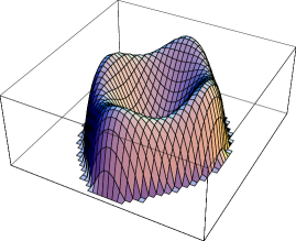
Figure 1: The $-U(\phi_{1},\phi_{2})$ potential (left) and the superpotential $W(\phi_{1},\phi_{2})$ (right)

The existence of the superpotential

$$W(\phi_{a})=2\left({1\over 3}\phi_{1}^{3}-{1\over 4}\phi_{1}+{\sigma\over 2}\phi_{1}\phi_{2}^{2}\right)\qquad,\qquad U(\phi_{1},\phi_{2})={1\over 2}\sum_{a=1}^{2}\,\frac{\partial W}{\partial\phi_{a}}\cdot\frac{\partial W}{\partial\phi_{a}}$$

allows for the Bogomolny splitting of the static energy:

$$E={4m^{3}\over\lambda}\int\,dx\,{1\over 2}\left[\sum_{a=1}^{2}\left(\frac{d\phi_{a}}{dx}\mp\frac{\partial W}{\partial\phi_{a}}\right)\left(\frac{d\phi_{a}}{dx}\mp\frac{\partial W}{\partial\phi_{a}}\right)\right]\pm{4m^{3}\over\lambda}\cdot\left\{W(\phi_{a}(+\infty))-W(\phi_{a}(-\infty))\right\}\qquad,$$ (9)

showing that the absolute minima of $E$ in each sector of ${\cal C}$ satisfy the first-order equations:

$${d\phi_{a}\over dx}=\pm\frac{\partial W}{\partial\phi_{a}}\qquad,\qquad\left\{\begin{array}[]{c}\qquad\displaystyle\frac{d\phi_{1}}{dx}=(-1)^{\alpha}(2\phi_{1}^{2}+\sigma\phi_{2}^{2}-{1\over 2})\\ \\ \displaystyle\frac{d\phi_{2}}{dx}=(-1)^{\beta}2\sigma\phi_{1}\phi_{2}\end{array}\right.\quad,\quad\alpha,\beta=0,1\qquad.$$ (10)

5.3.1 Kink flow lines

The solutions of (10) are the flow lines of the gradient of $W$, and those starting and ending at critical points of $W$ are the kink orbits.

                             

Figure 2: The $-U(\phi)=-{1\over 2}{\partial W\over\partial\phi_{1}}{\partial W\over\partial\phi_{1}}-{1\over 2}{\partial W\over\partial\phi_{2}}{\partial W\over\partial\phi_{2}}$ potential (left). Flow-lines: in the ranges $c\in(-\infty,c^{S})$ (middle left), $c=c^{S}$ (middle right), and $c\in(c^{S},\infty)$ (right)

.

The kink flow lines can be obtained analytically by integrating

$$(-1)^{\alpha}\frac{d\phi_{1}}{2\phi_{1}^{2}+\sigma\phi_{2}^{2}-{1\over 2}}+(-1)^{\beta}\frac{d\phi_{2}}{2\sigma\phi_{1}\phi_{2}}=0\qquad,$$

to find, after use of the integrating factor $|\phi_{2}|^{-{2\over\sigma}}$,

$$\phi_{1}^{2}+\frac{\sigma}{2(1-\sigma)}\phi_{2}^{2}=\frac{1}{4}+\frac{c}{2\sigma}|\phi_{2}|^{2\over\sigma}\hskip 28.45274pt,\,\sigma\neq 1\,,\hskip 28.45274ptc\in(-\infty,{1\over 4}{\sigma\over 1-\sigma}(2\sigma)^{{1+\sigma\over\sigma}})$$

$$\phi_{1}^{2}-\phi_{2}^{2}\left({c\over 2}+\ln|\phi_{2}|\right)={1\over 4}\hskip 28.45274pt,\,\sigma=1\,,\hskip 28.45274ptc\in(-\infty,-1+\ln 2)\qquad.$$

Thus, there exits a family of two-component topological kinks -TK2 kinks- parametrized by the integration constant $c$, all of them with the same energy:

$$E(\phi_{1}^{\pm(1)},\phi_{2}^{\pm(1)})=0\qquad,\qquad E(\phi_{1}^{K},\phi_{2}^{K})=\frac{4m^{3}}{\lambda}|W(\phi_{1}^{\pm(1)},\phi_{2}^{\pm(1)})-W(\phi_{1}^{\mp(1)},\phi_{2}^{\mp(1)})|=\frac{4m^{3}}{3\lambda}\qquad.$$

Note that there is a critical value $c^{S}={1\over 4}{\sigma\over 1-\sigma}(2\sigma)^{{1+\sigma\over\sigma}}$ if $\sigma\neq 1$, or, $c^{S}=-1+\ln 2$, if $\sigma=1$ beyond which the flow lines go to infinity and do not correspond to kink orbits because $W(|\vec{\phi}|(\infty))=\infty$ and the energy becomes infinite.

In general, the kink profile, the dependence on $x$ of the fields for a given kink orbit, cannot be expressed analytically. There are, however, two special kink orbits for which this is possible:

$$c=-\infty\quad,\quad\left\{\begin{array}[]{c}\phi_{1}^{{\rm TK1}}(x)=(-1)^{\alpha}{1\over 2}{\rm tanh}(x-a)\\ \phi_{2}^{{\rm TK1}}(x)=0\end{array}\right.\quad;\,\,\alpha=0,1\,,\,a\in{\mathbb{R}}$$

$$c=0\quad,\quad\left\{\begin{array}[]{c}\phi_{1}^{{\rm TK2}}(x)=(-1)^{\alpha_{1}}{1\over 2}{\rm tanh}[2(1-\sigma)(x-a)]\\ \phi_{2}^{{\rm TK2}}(x)=(-1)^{\alpha_{2}}\sqrt{{1-\sigma\over\sigma}}{\rm sech}[2(1-\sigma)(x-a)]\end{array}\right.\qquad,\qquad\alpha_{1},\alpha_{2}=0,1\qquad.$$

If $c=-\infty$, the orbit is a segment on the abscissa axis and one finds the very well known $\lambda(\phi)^{4}_{2}$ kink buried in the kink variety of the BNRT model. Since only one of the two components of the scalar field is different from zero, this kind of kink is termed TK1 kinks -one-component topological kinks- in the context of the BNRT model.

When $c=0$ things become more interesting. The kink orbit is a half-ellipse (if $\sigma\neq 1$) and the two components of the scalar field are not zero for this kind of topological -TK2- kink. Note that in both cases the kink profile is a function of a real parameter $a\in{\mathbb{R}}$, obeying the freedom of setting the kink center. This is a general feature shared with other kinks for which analytical expressions giving the kink profiles are not available. Therefore, the moduli space of kinks in the BNRT model is the two-dimensional manifold ${\cal M}_{K}^{2}=(-\infty,c^{S}]\times(-\infty,\infty)$ with coordinates $(c,a)$. That is, each kink in the BNRT model is determined by its orbit ($c\in(-\infty,c^{S}]$) and its center ($a\in(-\infty,\infty)$).

We close this subsection by enumerating the main features of non-generic kink orbits.

1. $c=-\infty$: The second component of the scalar field is zero and the kink orbit is invariant under the $\phi_{2}\rightarrow-\phi_{2}$ transformation. These orbits belongs to the ${\cal C}_{\pm}^{11}$ or ${\cal C}^{11}_{\mp}$ sectors.

2. $c=0$: The kink orbits are half-ellipses also living in the ${\cal C}_{\pm}^{11}$ or ${\cal C}^{11}_{\mp}$ sectors.

3. $c=c^{S}$: These orbits are the boundary between bounded and unbounded flow lines. They belong to ${\cal C}_{\pm}^{12}$, ${\cal C}^{12}_{\mp}$, ${\cal C}_{\pm}^{21}$ or ${\cal C}^{21}_{\mp}$ sectors.

5.3.2 Kink profiles from integrable systems

The search for finite energy static solutions in (1+1)-dimensional theories of two scalar fields is tantamount to investigating finite action trajectories in a mechanical system of two degrees of freedom. The potential energy of the mechanical system is equal to minus the potential energy density of the field theory. The mechanical analogue in this sense to the BNRT model is a Liouville integrable system if $\sigma={1\over 2}$ and $\sigma={1\over 2}$. Liouville systems are Hamilton-Jacobi separable and all the trajectories can be found. Here we shall describe only the $\sigma={1\over 2}$ case, where the HJ equation is separable using elliptic coordinates. Standard application of the HJ procedure provides the following formulas for all the kink profiles:

$$\phi_{1}^{{\rm TK}}[x;a,b]=(-1)^{{\alpha_{1}}}\left(\frac{1}{2}\frac{\sinh\left((x-a)\right)}{\cosh\left((x-a)\right)+b^{2}}\right)\hskip 14.22636pt,\hskip 14.22636pt\phi_{2}^{{\rm TK}}[x;a,b]=(-1)^{{\alpha_{2}}}\left(\frac{b}{\sqrt{b^{2}+\cosh\left((x-a)\right)}}\right)\qquad.$$

The variety of kinks depends on two integration constants: $a,b\in(-\infty,\infty)$. The second one, $b=\pm\sqrt{\frac{1}{\sqrt{1-4c}}}$, is determined by the constant $c\in(-\infty,{1\over 4})$, giving the kink orbit. In Figure 3 it is observed that upon increasing $b$ a splitting into two kinks arises.

Figure 3: Solitary waves corresponding to: (a) $b=0$, (b) $b=\sqrt{0.5}$, (c) $b=1$ and (d) $b=\sqrt{30}$.

This phenomenon is better understood by studying how the energy density varies with $b$. The energy density

$${\cal E}^{\rm TK}[x;0,b]=\sum_{a=1}^{2}\frac{\partial\phi_{a}^{\rm TK}}{\partial x}.\frac{\partial\phi_{a}^{\rm TK}}{\partial x}=\frac{4+7b^{2}{\rm cosh}[x]+4b^{4}{\rm cosh}[2x]+b^{2}{\rm cosh}[3x]}{2(b^{2}+{\rm cosh}[x])^{4}}$$

is shown in Figure 4.

Figure 4: Energy density ${\cal E}^{K}[x;0,b]$ for (a) $b=0$, (b) $b=\sqrt{0.5}$, (c) $b=1$ and (d) $b=\sqrt{30}$.

The critical points of ${\cal E}^{\rm TK}[x;0,b]$

$$\frac{\partial{\cal E}^{\rm TK}}{\partial x}[x;0,b]=\frac{2\sinh x}{(b^{2}+\cosh x)^{5}}\ P_{3}(\cosh x)\hskip 14.22636pt,\hskip 14.22636pt\frac{\partial{\cal E}^{\rm TK}}{\partial x}[x;0,b]=0$$

are the origin $x=0\simeq\sinh x=0,\,\forall b^{2}$ and the roots of the third-order polynomial $P_{3}(\cosh x)$:

$$P_{3}(\cosh x)=-b^{2}\cosh^{3}x-b^{4}\cosh^{2}x+(-3b^{2}+4b^{6})\cosh x+5b^{4}-4\qquad,$$

which under the change of variables $P_{3}(\cosh x)=-b^{2}\tilde{P}(u)$, $u^{2}(x)=-1+\cosh x$ becomes:

$$\tilde{P}(u)=(u^{2})^{3}+(b^{2}+3)(u^{2})^{2}-(4b^{4}-2b^{2}-6)(u^{2})-4\left(b^{4}+b^{2}-1-\frac{1}{b^{2}}\right)\qquad.$$

In sum, use of the Cardano-Vieta formulas to solve cubic algebraic equations prompts us to the following conclusions:

1. If $b^{2}\in[0,1]$ there are no real roots $P_{3}$. The only critical point of the energy density , a maximum, is the origin and only one lump of energy is carried by these kinks:

   $$\tilde{P}(u(x))\neq 0,\forall x,u(x)\in{\mathbb{R}}\qquad,\qquad{\cal E}^{\rm TK}[0;0,b]=\frac{2}{(b^{2}+1)^{2}}\qquad.$$

2. If $b^{2}>1$, $\tilde{P}(u)=0$ has two real solutions: $u_{\pm}=\pm\sqrt{r(b^{2})}\in{\mathbb{R}}$. The points

   $$x=\pm m(b^{2})\qquad,\qquad m(b^{2})=\frac{1}{2\sqrt{2}}{\rm arccosh}(1+r(b^{2}))$$

   are the maxima of ${\cal E}^{\rm TK}$ on the real line (the origin is now a minimum) and these kink profiles carry two lumps of energy . Understanding these two lumps as fundamental particles, $a$ is the center of mass whereas $b$ is the relative coordinate of this system of two particles that become glued when $b^{2}<1$.

5.3.3 Kink profiles: numerical methods

For generic values of $\sigma$ one must rely on numerical integration methods to find the profiles of the kink solutions. We do this by solving the first-order equations by standard numerical methods with “initial” conditions:

$$\phi_{1}(0)=0\qquad,\qquad\frac{\sigma}{2(1-\sigma)}\phi_{2}^{2}(0)-\frac{c}{2\sigma}|\phi_{2}(0)|^{\frac{2}{\sigma}}=\frac{1}{4}\qquad.$$

The reasons for this choice are twofold: (1) For any kink solution, $\phi_{1}(x)$ always has a zero. Translational invariance allows us to set the zero at $x=0$; (2) To ensure that we will find a numerical kink solution, we fix $\phi_{2}(0)$ on a kink orbit for a given value of $\sigma$ and arbitrary choices of $c$.

The numerical method provides us with a succession of points of the kink solution generated by an interpolation polynomial. The plots of the numerical results show that the behavior derived analytically for the kink profiles when $\sigma={1\over 2}$ is generic. For any value of $\sigma$ the kink profiles are composed of two kinks. The parameter $c$ giving the orbit is related to the kink separation. In some range of $c$ the two kinks melt into a single kink. The precise value of $c$ at which this happens depends on the value of $\sigma$. $\sigma={1\over 2}$ is singled out, because in this case $c=0$ is the value where two kinks fuse into a single kink, or, viceversa, a single kink splits into two kinks.

5.4 TK2 kink Casimir energy

Small kink deformations $\phi_{a}(x)=\phi_{a}^{\rm TK}(x;c)+\delta\phi_{a}(x)$ are still solutions of the first-order equations if $\delta\phi_{a}(x)\in{\rm Ker}\,D(c)$:

$$D(c)\delta\vec{\phi}(x)=\left(\begin{array}[]{cc}-{d\over dx}-4\bar{\phi}_{1}(x;c)&-2\sigma\bar{\phi}_{2}(x;c)\\ -2\sigma\bar{\phi}_{2}(x;c)&-{d\over dx}-2\sigma\bar{\phi}_{1}(x;c)\end{array}\right)\left(\begin{array}[]{c}\delta\phi_{1}(x)\\ \delta\phi_{2}(x)\end{array}\right)=\left(\begin{array}[]{c}0\\ 0\end{array}\right)\qquad.$$

We shall use the notation $\vec{\phi}^{\rm TK}(x;c)=\bar{\phi}_{1}^{\rm TK}(x;c)\vec{e}_{1}+\bar{\phi}_{2}^{\rm TK}(x;c)\vec{e}_{2}$ because no analytic expressions for the kink profiles are known (except for some special values of $\sigma$). The $c$ parameter tells us what kink orbit is chosen. Note that:

$$K^{-}(c)=\left(\begin{array}[]{cc}-\frac{d^{2}}{dx^{2}}+8\bar{\phi}_{1}^{2}(x;c)+4\sigma(\sigma-1)\bar{\phi}_{2}^{2}(x;c)+2&8\sigma\bar{\phi}_{1}(x;c)\bar{\phi_{2}}(x;c)\\ 8\sigma\bar{\phi}_{1}(x;c)\bar{\phi_{2}}(x;c)&-\frac{d^{2}}{dx^{2}}+4\sigma(\sigma-1)\bar{\phi}_{1}^{2}(x;c)+2\sigma^{2}\bar{\phi}_{2}^{2}(x;c)+\sigma\end{array}\right)$$

$$K(c)=\left(\begin{array}[]{cc}-\frac{d^{2}}{dx^{2}}+24\bar{\phi}_{1}^{2}(x;c)+4\sigma(\sigma+1)\bar{\phi}_{2}^{2}(x;c)-2&8\sigma(\sigma+1)\bar{\phi}_{1}(x;c)\bar{\phi_{2}}(x;c)\\ 8\sigma(\sigma+1)\bar{\phi}_{1}(x;c)\bar{\phi_{2}}(x;c)&-\frac{d^{2}}{dx^{2}}+4\sigma(\sigma+1)\bar{\phi}_{1}^{2}(x;c)+6\sigma^{2}\bar{\phi}_{2}^{2}(x;c)-\sigma\end{array}\right)\quad,$$

if $\alpha=\beta$. For $\alpha\neq\beta$, $K^{-}(c)=D^{\dagger}(c)D(c)$ and $K(c)=D(c)D^{\dagger}(c)$ are exchanged.

Moreover, the shift of the Higgs and Goldstone fields from the stable kink solution, $\vec{\phi}(x^{\mu})=\vec{\phi}^{\rm TK}(x;c)+H(x^{\mu})\vec{e}_{1}+G(x^{\mu})\vec{e}_{2}$, causes the action in the kink sector to be the complicated expression:

$$S = -\frac{4m^{3}}{3\lambda}\lim_{T\rightarrow\infty}\int_{-\frac{T}{2}}^{\frac{T}{2}}\,dx_{0}\,+\frac{m^{2}}{\lambda}\int d^{2}x\left[{1\over 2}\partial_{\mu}H\partial^{\mu}H-\left(12\bar{\phi}^{2}_{1}(x;c)+2\sigma(\sigma+1)\bar{\phi}_{2}^{2}(x;c)-1\right)H^{2}(x^{\mu})\right]$$

$$+ \frac{m^{2}}{\lambda}\int d^{2}x\left[{1\over 2}\partial_{\mu}G\partial^{\mu}G-\left(2\sigma(\sigma+1)\bar{\phi}^{2}_{1}(x;c)+3\sigma^{2}\bar{\phi}_{2}^{2}(x;c)-{\sigma\over 2}\right)G^{2}(x^{\mu})\right]$$

$$- {m^{2}\over\lambda}\int d^{2}x\left[8\sigma(\sigma+1)\bar{\phi}_{1}(x;c)\bar{\phi}_{2}(x;c)H(x^{\mu})G(x^{\mu})\right.+$$

$$+ \left.2H^{4}(x^{\mu})+2\sigma(\sigma+1)H^{2}(x^{\mu})G^{2}(x^{\mu})+{\sigma^{2}\over 2}G^{4}(x^{\mu})\right]$$

$$- {m^{2}\over\lambda}\int d^{2}x\left[8\bar{\phi}_{1}(x;c)H^{3}(x^{\mu})+4\sigma(\sigma+1)\bar{\phi}_{1}(x;c)H(x^{\mu})G^{2}(x^{\mu})+\right.$$

$$\hskip 62.59596pt\left.+4\sigma(\sigma+1)\bar{\phi}_{2}(x;c)H^{2}(x^{\mu})G(x^{\mu})+2\sigma^{2}\bar{\phi}_{2}(x;c)G^{3}(x^{\mu})\right]\qquad.$$

Both the Higgs and Goldstone propagators, as well as all the trivalent vertices, are distorted by the kink. In the background of a TK2 kink, Higgs and Goldstone particles can transform into each other by means of the bivalent vertex induced.

Thus, the classical energy for small fluctuations $\vec{\phi}(x_{0},x)=\vec{\phi}^{\rm TK}(x;c)+\delta H(x_{0},x)\vec{e}_{1}+\delta G(x_{0},x)\vec{e}_{2}$ reads:

$$H^{(2)} = \frac{2m^{3}}{\lambda}\int\,dx\,\left[\frac{\partial\delta H}{\partial x_{0}}\cdot\frac{\partial\delta H}{\partial x_{0}}+\delta H(x_{0},x)K_{11}(c)\delta H(x_{0},x)+\delta H(x_{0},x)K_{12}(c)\delta G(x_{0},x)\right.+$$

$$+ \left.\delta G(x_{0},x)K_{21}(c)\delta H(x_{0},x)+\delta G(x_{0},x)K_{22}(c)\delta G(x_{0},x)\frac{}{}\right]\qquad,$$

where $K_{ab}(c)$ are the matrix elements of the second order fluctuation operator, which we rewrite, together with his supersymmetric partner, in the form:

$$K(c)=D(c)D^{\dagger}(c)=\left(\begin{array}[]{cc}-{d^{2}\over dx^{2}}+4+V_{11}(x;c)&V_{12}(x;c)\\ V_{21}(x;c)&-{d^{2}\over dx^{2}}+\sigma^{2}+V_{22}(x;c)\end{array}\right)\qquad,$$

$$\qquad K^{-}=D^{\dagger}(c)D(c)=\left(\begin{array}[]{cc}-{d^{2}\over dx^{2}}+4+V_{11}^{-}(x;c)&V_{12}^{-}(x;c)\\ V_{21}^{-}(x;c)&-{d^{2}\over dx^{2}}+\sigma^{2}+V_{22}^{-}(x;c)\end{array}\right)\qquad,$$

$$V_{11}(x;c) = 24\bar{\phi}_{1}^{2}(x;c)+4\sigma(\sigma+1)\bar{\phi}_{2}^{2}(x;c)-6$$

$$V_{12}(x;c) = 8\sigma(\sigma+1)\bar{\phi}_{1}(x;c)\bar{\phi}_{2}(x;c)=V_{21}(x;c)$$

$$V_{22}(x;c) = 4\sigma(\sigma+1)\bar{\phi}_{1}^{2}(x;c)+6\sigma^{2}\bar{\phi}_{2}^{2}(x;c)-\sigma(\sigma+1)$$

$$V_{11}^{-}(x;c) = 8\bar{\phi}_{1}^{2}(x;c)+4\sigma(\sigma-1)\bar{\phi}_{2}^{2}(x;c)-2$$

$$V_{12}^{-}(x;c) = 8\sigma\bar{\phi}(x;c)\bar{\phi}_{2}(x;c)=V_{21}^{-}(x;c)$$

$$V_{22}^{-}(x;c) = 4\sigma(\sigma-1)\bar{\phi}_{1}^{2}(x;c)+2\sigma^{2}\bar{\phi}_{2}^{2}(x;c)-\sigma(\sigma+1)$$

For instance, the family of Hessian operators for the topological kinks found in the $\sigma={1\over 2}$ case can be written explicitly:

$$K(b)=\left(\begin{array}[]{cc}-\frac{d^{2}}{dx^{2}}+\frac{3b}{\cosh x+b}+\frac{6\sinh^{2}x}{(\cosh x+b)^{2}}-2&\frac{6\sqrt{b}\sinh x}{(\cosh x+b)^{\frac{3}{2}}}\\ \frac{6\sqrt{b}\sinh x}{(\cosh x+b)^{\frac{3}{2}}}&-\frac{d^{2}}{dx^{2}}+\frac{3}{2}\frac{b}{\cosh x+b}+\frac{3}{4}\frac{\sinh^{2}x}{(\cosh x+b)^{2}}-\frac{1}{2}\end{array}\right)\qquad.$$

 

  

Figure 5: Diagonal components $V_{11}(x)$ (red) and $V_{22}(x)$ (green) of the potential for c=-30, c=-1, c=0.1, c=0.245 and c=0.249.

In any case, the spectral resolution of

$$K(c)f_{\varepsilon}(x)=\varepsilon^{2}f_{\varepsilon}(x)\hskip 28.45274pt,\hskip 28.45274pt\lim_{x\rightarrow\pm\infty}K(c)=K_{0}$$

for any value of $\sigma$ has the following features:

1. The kernel of $K(c)$ is of dimension two and the orthogonal basis is provided by the two eigenfunctions (zero modes):

   $$\varepsilon=0\qquad;\qquad f_{0}^{(1)}(x)=\left(\begin{array}[]{c}\frac{\partial\phi_{1}^{\rm TK}}{\partial x}(x)\\[5.69046pt] \frac{\partial\phi_{2}^{\rm TK}}{\partial x}(x)\end{array}\right)\qquad\qquad,\qquad\qquad f_{0}^{(2)}(x)=\left(\begin{array}[]{c}\frac{\partial\phi_{1}^{\rm TK}}{\partial c}(x)\\[5.69046pt] \frac{\partial\phi_{2}^{\rm TK}}{\partial c}(x)\end{array}\right)\qquad,$$

   obeying the fact that motion in the kink moduli space costs no energy: all the kink solutions are in neutral equilibrium.

2. There are bound states in a number, $N(c)$, that depends on $c$.

   $$\varepsilon^{2}=\varepsilon_{l}>0,\,\,l=1,2,\cdots,N(c)\quad;\quad f_{\varepsilon_{l}}(x)=\left(\begin{array}[]{c}f_{1}^{\varepsilon_{l}}(x)\\ f_{2}^{\varepsilon_{l}}(x)\end{array}\right)\quad,\quad\int\,dx\,f_{\varepsilon_{l}}^{T}(x)f_{\varepsilon_{m}}(x)=\delta^{lm}\quad.$$

3. There are two branches of scattering states:

   $$(1)\quad\varepsilon^{2}=k^{2}+4\quad;\quad f_{\varepsilon}^{(1)}(x;k))=e^{-ikx}\left(\begin{array}[]{c}u_{1}^{(1)}(x;k)\\ u_{2}^{(1)}(x;k)\end{array}\right)\quad,\quad\lim_{x\rightarrow\pm\infty}\left(\begin{array}[]{c}u_{1}^{(1)}(x;k)=u_{1}^{\pm}(k)\\ u_{2}^{(1)}(x;k)=0\end{array}\right)\quad.$$

   In terms of non-explicitly known phase shifts -determined by $u_{1}^{\pm}(k)$-, Periodic Boundary Conditions in the interval $I=[-\frac{mL}{2},\frac{mL}{2}]$ give the spectral densities in ${\rm Spec}K(c)$:

   $$k\cdot mL+\delta_{1}(k)=2\pi n\qquad,\qquad\rho_{1}^{\rm TK}(k)={1\over 2\pi}(mL+\frac{d\delta_{1}(k)}{dk})\qquad.$$

   $$(2)\quad\lambda^{2}=q^{2}+\sigma^{2}\quad;\quad f_{\lambda}^{(2)}(x;q))=e^{-iqx}\left(\begin{array}[]{c}u_{1}^{(2)}(x;q)\\ u_{2}^{(2)}(x;q)\end{array}\right)\quad,\quad\lim_{x\rightarrow\pm\infty}\left(\begin{array}[]{c}u_{1}^{(2)}(x;q)=0\\ u_{2}^{(2)}(x;q)=u_{2}^{\pm}(q)\end{array}\right)\quad.$$

   The phase shifts are now read from $u_{2}^{\pm}(q)$ and the PBC give the spectral densities in the other branch of ${\rm Spec}K(c)$:

   $$q\cdot mL+\delta_{2}(q)=2\pi n\qquad,\qquad\rho_{2}^{\rm TK}(q)={1\over 2\pi}(mL+\frac{d\delta_{2}(q)}{dq})\qquad.$$

The eigenfunctions in the continuous spectrum of $K(c)$ also satisfy orthogonality conditions:

$$\int\,dx\,f_{\varepsilon}^{\dagger(I)}(x;k)f_{\varepsilon^{\prime}}^{(J)}(x;q)=\delta^{IJ}\delta_{kq}\qquad,\qquad I,J=1,2\qquad.$$

The general solution to the linearized field equations

$$\frac{\partial^{2}\delta H}{\partial x_{0}^{2}}-\frac{\partial^{2}\delta H}{\partial x^{2}}+(24\bar{\phi}_{1}^{2}(x;c)+4\sigma(\sigma+1)\bar{\phi}_{2}^{2}(x;c)-2)\delta H(x^{\mu})+8\sigma(\sigma+1)\bar{\phi}_{1}(x;c)\bar{\phi}_{2}(x;c)\delta G(x^{\mu})=0$$

$$\frac{\partial^{2}\delta G}{\partial x_{0}^{2}}-\frac{\partial^{2}\delta G}{\partial x^{2}}+8\sigma(\sigma+1)\bar{\phi}_{1}(x;c)\bar{\phi}_{2}(x;c)\delta H(x^{\mu})+(4(\sigma(\sigma+1)\bar{\phi}_{1}^{2}(x;c)+6\sigma^{2}\bar{\phi}_{2}^{2}(x;c)-\sigma)\delta G(x^{\mu})=0$$

is a linear combination of the eigen-functions of $K(c)$ :

$$\left(\begin{array}[]{c}\delta H^{\prime}(x_{0},x)\\ \delta G^{\prime}(x_{0},x)\end{array}\right) = \frac{\sqrt{\lambda}}{2m}\cdot\sqrt{\frac{\hbar}{mL}}\cdot\left\{\sum_{l=1}^{N(c)}\frac{1}{\sqrt{2\sqrt{\varepsilon_{l}}}}\left(A^{l}e^{-i\varepsilon_{l}x_{0}}+A^{*l}e^{i\varepsilon_{l}x_{0}}\right)f_{\varepsilon_{l}}(x)+\right.$$

$$+ \sum_{k}\frac{1}{\sqrt{2\varepsilon(k)}}\left\{A^{(1)}(k)e^{-i\varepsilon(k)x_{0}}f_{\varepsilon}^{(1)}(x)+A^{*(1)}(k)e^{i\varepsilon(k)x_{0}}f_{\varepsilon}^{(1)*}(x)\right\}+$$

$$+ \left.\sum_{q}\frac{1}{\sqrt{2\lambda(q)}}\left\{A^{(2)}(q)e^{-i\lambda(q)x_{0}}f^{(2)}_{\lambda}(x)+A^{*(2)}(q)e^{i\lambda(q)x_{0}}f_{\lambda}^{*(2)}(x)\right\}\right\}\qquad.$$

The classical free Hamiltonian for kink fluctuations becomes:

$$H^{(2)} = \frac{\hbar m}{2}\left\{\sum_{l=1}^{N(c)}\sqrt{\varepsilon_{l}}(A^{*l}A^{l}+A^{l}A^{*l})+\sum_{k}\varepsilon(k)(A^{(1)*}(k)A^{(1)}(k)+A^{(1)}(k)A^{(1)*}(k))+\right.$$

$$+ \left.\sum_{q}\lambda(q)(A^{(2)*}(q)A^{(2)}(q)+A^{(2)}(q)A^{(2)*}(q))\right\}$$

and, after canonical quantization,

$$[A^{l},A^{m\dagger}]=\delta_{lm}\qquad,\qquad[A^{(I)}(k),A^{(J)\dagger}(q)]=\delta^{IJ}\delta_{kq}$$

one obtains the quantum free Hamiltonian

$$\hat{H}^{(2)}=\hbar m\left\{\sum_{l=1}^{N(c)}\sqrt{\varepsilon_{l}}\left(\hat{A}^{l\dagger}\hat{A}^{l}+{1\over 2}\right)+\sum_{k}\varepsilon(k)\left(\hat{A}^{(1)\dagger}(k)\hat{A}^{(1)}(k)+{1\over 2}\right)+\sum_{k}\lambda(k)\left(\hat{A}^{(2)\dagger}(k)\hat{A}^{(2)}(k)+{1\over 2}\right)\right\}$$

and the kink Casimir energy

$$\Delta E(\vec{\phi}^{\rm TK}(c))={\hbar m\over 2}\left(\sum_{l=1}^{N(c)}\sqrt{\varepsilon_{l}}+\sum_{k}\varepsilon(k)+\sum_{q}\lambda(q)\right)={\hbar m\over 2}{\rm Tr}K(c)^{{1\over 2}}$$

when all the positive modes are non-occupied.

In sum, the TK2 kink semi-classical energy -one-loop order- receives three contributions:

1. The classical energy $E(\vec{\phi}^{\rm TK}(c))=\frac{4m^{3}}{3\lambda}$.

2. The TK2 kink Casimir energy -zero point energy renormalization-

   $$\Delta M_{K}^{C}(c)=\Delta E(\vec{\phi}^{\rm TK}(c))-\Delta E(\vec{\phi}^{\pm(1)})={\hbar m\over 2}\left({\rm Tr}K(c)^{{1\over 2}}-{\rm Tr}K_{0}^{{1\over 2}}\right)\qquad.$$

3. The contribution of ${\cal L}_{C.T.}$ to one-loop TK2 kink masses is:

   $$\Delta M_{K}^{R}(c)= - \frac{\hbar m}{2}\int\,dx\left\{\left[6\cdot I(4)+\sigma(\sigma+1)\cdot I(\sigma^{2})\right][(\phi_{1}^{\rm TK}(x,c))^{2}-(\phi_{1}^{(1)})^{2}]\right\}-$$

   $$- \frac{\hbar m}{2}\int\,dx\left\{\left[4\sigma(\sigma+1)\cdot I(4)+6\sigma^{2}\cdot I(\sigma^{2})\right][(\phi_{2}^{\rm TK}(x,c))^{2}-(\phi_{2}^{(1)})^{2}]\right\}\qquad.$$

Therefore, the one-loop TK2 kink mass and the semi-classical kink energy are the divergent quantities:

$$\Delta M_{K}(c)=\Delta M_{K}^{C}(c)+\Delta M_{K}^{R}(c)\qquad,\qquad E_{S}(\vec{\phi}^{\rm TK}(c)=E(\vec{\phi}^{\rm TK}(c))+\Delta M_{K}(c)\qquad.$$

6 The TK2 kink heat kernel and generalized zeta function

6.1 Zeta function regularization

We regularize the ultraviolet divergent TK2 kink and vacuum energies in terms of their generalized zeta functions:

$$\Delta M_{K}^{C}(c,s)={\hbar\over 2}({\mu^{2}\over m^{2}})^{s}\mu\left(\zeta_{K}(c)(s)-\zeta_{K_{0}}(s)\right)\qquad.$$

Here, $s$ is the non-dimensional complex parameter already introduced in the previous Lecture; the auxiliary parameter $\mu$ of $L^{-1}$ dimensions has also been used in the previous Lecture to keep the dimensions in order in the regularization procedure, and the generalized zeta functions are the series:

$$\zeta_{K(c)}(s)=\sum_{l=1}^{N(c)}\,{1\over\varepsilon_{l}^{2s}}+\sum_{k}\,{1\over\varepsilon(k)^{2s}}+\sum_{q}\,{1\over\lambda(q)^{2s}}\qquad,\qquad\zeta_{K_{0}}(s)=\sum_{k}\,{1\over\omega(k)^{2s}}+\sum_{q}\,{1\over\gamma(q)^{2s}}\qquad.$$

Therefore,

$$\Delta M_{K}^{C}(c)=\lim_{s\rightarrow-{1\over 2}}\Delta M_{K}^{C}(c,s)={\hbar m\over 2}\left(\zeta_{K}(c)(-{1\over 2})-\zeta_{K_{0}}(-{1\over 2})\right)\qquad,$$

and the divergences reappear at $s=-{1\over 2}$, which is a pole of the meromorphic function $\Delta M_{K}^{C}(c,s)$ of the complex parameter s.

$\Delta M_{K}^{R}(c)$ can also be regularized in terms of generalized zeta functions. Both divergent integrals $I(4)$ and $I(\sigma^{2})$ when the system is considered in the interval $I=-[{mL\over 2},{mL\over 2}]$ become the divergent series

$$I(4)={1\over 2}{1\over mL}\sum_{n}\,\frac{1}{\sqrt{{n^{2}\over R^{2}}+4}}\qquad,\qquad I(\sigma^{2})={1\over 2}{1\over mL}\sum_{n}\,\frac{1}{\sqrt{{n^{2}\over R^{2}}+\sigma^{2}}}\qquad.$$

Thus, they are obtained as the limits:

$$I(4) = -\lim_{s\rightarrow-{1\over 2}}\frac{1}{\mu L}\cdot\frac{\Gamma(s+1)}{\Gamma(s)}\cdot\left(\frac{\mu^{2}}{m^{2}}\right)^{s+1}\cdot\zeta_{K_{0}^{11}}(s+1)\quad,\quad K_{0}^{11}=-\frac{d^{2}}{dx^{2}}+4$$

$$I(\sigma^{2}) = -\lim_{s\rightarrow-{1\over 2}}\frac{1}{\mu L}\cdot\frac{\Gamma(s+1)}{\Gamma(s)}\cdot\left(\frac{\mu^{2}}{m^{2}}\right)^{s+1}\cdot\zeta_{K_{0}^{22}}(s+1)\quad,\quad K_{0}^{22}=-\frac{d^{2}}{dx^{2}}+\sigma^{2}\qquad.$$

The regularized contribution of the mass renormalization counter-terms to the kink mass is:

$$\Delta M_{K}^{R}(c,s) = \frac{\hbar}{2L}\lim_{s\rightarrow-{1\over 2}}\,\frac{\Gamma(s+1)}{\Gamma(s)}\cdot\left(\frac{\mu^{2}}{m^{2}}\right)^{s+\frac{1}{2}}\cdot$$

$$\cdot \left\{[6\zeta_{K_{0}^{11}}(s+1)+\sigma(\sigma+1)\zeta_{K_{0}^{22}}(s+1)]\int\,dx\,\left[(\phi_{1}^{\rm TK}(x,c))^{2}-(\phi_{1}^{(1)})^{2}\right]\right.+$$

$$+ \left.[4\sigma(\sigma+1)\zeta_{K_{0}^{11}}(s+1)+6\sigma^{2}\zeta_{K_{0}^{22}}(s+1)]\int\,dx\,\left[(\phi_{2}^{\rm TK}(x,c))^{2}-(\phi_{2}^{(1)})^{2}\right]\right\}\qquad.$$

Therefore,

$$\Delta M_{K}^{C}(c) = \lim_{s\rightarrow-{1\over 2}}\Delta M_{K}^{R}(c,s)$$

$$= -\frac{\hbar}{4L}\left\{[6\zeta_{K_{0}^{11}}({1\over 2})+\sigma(\sigma+1)\zeta_{K_{0}^{22}}({1\over 2})]\int\,dx\,\left[(\phi_{1}^{\rm TK}(x,c))^{2}-(\phi_{1}^{(1)})^{2}\right]\right.+$$

$$+ \left.[4\sigma(\sigma+1)\zeta_{K_{0}^{11}}({1\over 2})+6\sigma^{2}\zeta_{K_{0}^{22}}({1\over 2})]\int\,dx\,\left[(\phi_{2}^{\rm TK}(x,c))^{2}-(\phi_{2}^{(1)})^{2}\right]\right\}\qquad.$$

6.2 The Cahill-Comtet-Glauber (CCG) exact formula

The goal in this sub-Section is to compute the one-loop mass shift for the one-component TK1 topological kink:

$$\phi_{1}^{{\rm TK}1}(x;c=-\infty)={1\over 2}{\rm tanh}x\hskip 42.67912pt,\hskip 42.67912pt\phi_{2}^{{\rm TK}1}(x;c=-\infty)=0\qquad.$$

The Kink fluctuation operator -$K(-\infty)=K$ for short- is diagonal for any value of $\sigma$:

$$K=\left(\begin{array}[]{cc}K^{11}&0\\ 0&K^{22}\end{array}\right)=\left(\begin{array}[]{cc}-\frac{d^{2}}{dx^{2}}+4-\frac{6}{{\rm cosh}^{2}x}&0\\ 0&-\frac{d^{2}}{dx^{2}}+\sigma^{2}-\frac{\sigma(\sigma+1)}{{\rm cosh}^{2}x}\end{array}\right)\qquad.$$

Both diagonal entries $K^{11}$ and $K^{22}$ are Posch-Teller Schrodinger operators with very well known spectra.

I. The spectrum of $K^{11}$:

There are three types of eigenfunctions

1. Bound states:

   $$\varepsilon_{0}=0\hskip 42.67912pt,\hskip 42.67912pt\psi_{0}(x)={1\over{\rm cosh}^{2}x}$$

   $$\varepsilon_{1}=3\hskip 42.67912pt,\hskip 42.67912pt\psi_{3}(x)={{\rm sinh}x\over{\rm cosh}^{2}x}$$

2. Scattering states:

   $$\varepsilon^{2}(k)=k^{2}+4\hskip 42.67912pt,\hskip 42.67912pt\psi_{k}(x)=e^{ikx}P_{2}({\rm tanh}x;k)\quad,\quad P_{2}(z;k)=3z^{2}-1-3ikz-k^{2}\qquad,$$

   with phase shifts:

   $$\delta_{1}(k)=-2{\rm arctan}\frac{3k}{2-k^{2}}\qquad.$$

3. Half-bound state:

   $$\varepsilon_{1\over 2}=4\hskip 42.67912pt,\hskip 42.67912pt\psi_{(k=0)}(x)=P_{2}({\rm tanh}x;0)\qquad.$$

II. The spectrum of $K^{22}$:

1. Bound states: $l=0,1,2,\cdots,N,\qquad N=I[\sigma]$

   $$\varepsilon_{l}=(2\sigma-l)l\hskip 42.67912pt,\hskip 42.67912pt\psi_{l}(x)=\frac{1}{({\rm cosh}x)^{\sigma-l}}\,{}_{2}F_{1}[-l,2\sigma-l,\sigma-l+1;{1\over 2}(1+{\rm tanh}x)]$$

2. Scattering states:

   $$\varepsilon=q^{2}+\sigma^{2}\hskip 42.67912pt,\hskip 42.67912pt\psi_{q}(x)=e^{iqx}\,{}_{2}F_{1}[-\sigma,\sigma,1-iq;\frac{e^{x}}{e^{x}+e^{-x}}]\qquad.$$

   From these wave functions, one reads the following transmission and reflection scattering coefficients:

   $$T(q)=\frac{\Gamma(\sigma+1-iq)\Gamma(-\sigma-iq)}{\Gamma(1-iq)\Gamma(-iq)}\qquad,\qquad R(q)=\frac{\Gamma(\sigma+1-iq)\Gamma(-\sigma-iq)\Gamma(iq)}{\Gamma(1+\sigma)\Gamma(-\sigma)\Gamma(-iq)}\qquad.$$

   Henceforth, the phase shifts

   $$\delta_{2}(q)=\delta_{2}^{+}(q)+\delta_{2}^{-}(q)\qquad;\qquad\delta_{2}^{\pm}(q)={1\over 4}{\rm arctan}\left(\frac{{\rm Im}(T(q)\pm R(q))}{{\rm Re}(T(q)\pm R(q)}\right)$$

   identify these scattering processes.

   If $\sigma=N\in{\mathbb{N}}$ is a natural number, $R(q)=0$, $\delta_{2}^{+}(q)=\delta_{2}^{-}(q)$, and the total phase shift $\delta_{2}(q)=\delta_{2}^{+}(q)+\delta_{2}^{-}(q)$ is:

   $$\delta_{2}(q)=\frac{1}{2}{\rm arctan}\left(\frac{{\rm Im}\prod_{n=0}^{N-1}(q^{2}-(N-n)^{2}+2iq(N-n))}{{\rm Re}\prod_{n=0}^{N-1}(q^{2}-(N-n)^{2}+2iq(N-n))}\right)$$

3. Half-bound state: If $\sigma=I[\sigma]=N\in{\mathbb{N}}$

   $$\varepsilon_{1\over 2}=N^{2}\qquad\quad,\qquad\quad\psi_{q=0}(x)={}_{2}F_{1}[-\sigma,\sigma,1;\frac{1}{2}(1+{\rm tanh}x)]$$

   also belongs to the spectrum.

Thus, one expects that the one-loop TK1 mass shift can be calculated exactly from this complete spectral information. We distinguish, however, two different situations according to whether or not $\sigma$ is a (positive) integer.

6.2.1 $\sigma=N\in{\mathbb{N}}$: one-loop TK1 mass shift from bound states

If $\sigma$ is a natural number, the reflection scattering coefficient is zero for both $K^{11}$ and $K^{22}$. The Cahill-Comtet-Glauber (CCG) formula can be applied. This formula gives the one-loop mass shift of one-dimensional solitons from the energies of their bound states. Applied to the TK1 kink of the BNRT model it reads:

$$\Delta M(\vec{\phi}^{\,TK1})=-\frac{\hbar m}{\pi}\left(\sum_{i=0}^{1}\,2({\rm sin}\theta_{i}-\theta_{i}{\rm cos}\theta_{i})+\sum_{l=0}^{N-1}\,N({\rm sin}\alpha_{l}-\alpha_{l}{\rm cos}\alpha_{l})\right)\qquad.$$ (14)

The angles are defined in terms of the eigenvalues of the bound states of $K^{11}$ and $K^{22}$:

$$\theta_{0}={\rm arccos}({0\over 2})={\pi\over 2}\quad,\quad\theta_{1}={\rm arccos}({\sqrt{3}\over 2})={\pi\over 6}\quad,\quad\alpha_{l}={\rm arccos}(\frac{\sqrt{(2N-l)l}}{N})\quad.$$

Thus, for the first five cases we obtain:

1. $\sigma=1$

   $$\alpha_{0}={\pi\over 2}\quad,\quad{\rm sin}\theta_{0}={\rm sin}\alpha_{0}=1\qquad,\qquad{\rm sin}\theta_{1}={1\over 2}$$

   $$\Delta M(\vec{\phi}^{\,TK1})=(-{3\over\pi}+{1\over 2\sqrt{3}})\hbar m-{1\over\pi}\hbar m=-0.984564\hbar m\qquad.$$

2. $\sigma=2$

   $$\alpha_{1}={\pi\over 6}\qquad\qquad,\qquad\Delta M(\vec{\phi}^{\,TK1})=(-{3\over\pi}+{1\over 2\sqrt{3}})\hbar m-({3\over\pi}-{1\over 2\sqrt{3}})\hbar m=-1.33251\hbar m\qquad.$$

3. $\sigma=3$

   $$\alpha_{1}={\rm arccos}({\sqrt{5}\over 3})\quad,\quad{\rm sin}\alpha_{1}={2\over 3}\qquad,\qquad\alpha_{2}={\rm arccos}(2{\sqrt{2}\over 3})\quad,\quad{\rm sin}\alpha_{2}={1\over 3}$$

   $$\Delta M(\vec{\phi}^{\,TK1})=(-{3\over\pi}+{1\over 2\sqrt{3}})\hbar m-({6\over\pi}-{1\over\pi}(\sqrt{5}{\rm arccos}({\sqrt{5}\over 3})+2\sqrt{2}{\rm arccos}(2{\sqrt{2}\over 3})))\hbar m=-1.75076\hbar m\qquad.$$

4. $\sigma=4$

   $$\alpha_{1}={\rm arccos}({\sqrt{7}\over 4})\quad,\quad{\rm sin}\alpha_{1}={3\over 4}\qquad \qquad\alpha_{2}={\rm arccos}(2{\sqrt{3}\over 4})\quad,\quad{\rm sin}\alpha_{2}={2\over 4}$$ ,

   $$\alpha_{3}={\rm arccos}({\sqrt{15}\over 4})\quad \quad{\rm sin}\alpha_{3}={1\over 4}$$ ,

   $$\Delta M(\vec{\phi}^{\,TK1}) = (-{3\over\pi}+{1\over 2\sqrt{3}})\hbar m-({10\over\pi}-{1\over\pi}(\sqrt{7}{\rm arccos}({\sqrt{7}\over 4})+2\sqrt{3}{\rm arccos}({2\sqrt{3}\over 4})+$$

   $$+ \sqrt{15}{\rm arccos}({\sqrt{15}\over 4})))\hbar m=-2.24628\hbar m\qquad.$$

5. $\sigma=5$

   $$\alpha_{1}={\rm arccos}({\sqrt{9}\over 5})\quad,\quad{\rm sin}\alpha_{1}={4\over 5}\qquad \qquad\alpha_{2}={\rm arccos}(2{\sqrt{4}\over 5})\quad,\quad{\rm sin}\alpha_{2}={3\over 5}$$ ,

   $$\alpha_{3}={\rm arccos}({\sqrt{21}\over 5})\quad,\quad{\rm sin}\alpha_{3}={2\over 5}\quad \quad\alpha_{4}={\rm arccos}({2\sqrt{6}\over 5})\quad,\quad{\rm sin}\alpha_{4}={1\over 5}$$ ,

   $$\Delta M(\vec{\phi}^{\,TK1}) = (-{3\over\pi}+{1\over 2\sqrt{3}})\hbar m-({15\over\pi}-{1\over\pi}(\sqrt{9}{\rm arccos}({\sqrt{9}\over 5})+2\sqrt{4}{\rm arccos}({2\sqrt{4}\over 5})+$$

   $$+ \sqrt{21}{\rm arccos}({\sqrt{21}\over 5})+2\sqrt{6}{\rm arccos}({2\sqrt{6}\over 5})))\hbar m=-2.82180\hbar m\qquad.$$

6.2.2 $\sigma\in{\mathbb{R}}^{+}$: one-loop TK1 mass shift from zeta functions

The partition and generalized zeta functions for the vacuum operator $K_{0}$ are at the $R\rightarrow\infty$ limit respectively:

$${\rm Tr}e^{-\beta K_{0}} = \frac{mL}{2\pi}\left[\int_{-\infty}^{+\infty}\,dk\,e^{-\beta(k^{2}+4)}+\int_{-\infty}^{+\infty}\,dq\,e^{-\beta(q^{2}+\sigma^{2})}\right]=\frac{mL}{\sqrt{4\pi\beta}}\cdot\left[e^{-4\beta}+e^{-\sigma^{2}\beta}\right]$$

$$\zeta_{K_{0}}(s) = {mL\over\sqrt{4\pi}}\cdot{1\over\Gamma(s)}\cdot\int_{0}^{\infty}\,d\beta\,\beta^{s-{3\over 2}}\,\left[e^{-4\beta}+e^{-\sigma^{2}\beta}\right]={mL\over\sqrt{4\pi}}\cdot\left[{1\over 2^{2s-1}}+{1\over\sigma^{2s-1}}\right]\cdot\frac{\Gamma(s-{1\over 2})}{\Gamma(s)}\qquad.$$

The poles of $\zeta_{K_{0}}(x)$ are thus the poles of the Euler Gamma function $\Gamma(s-{1\over 2})$: $s-{1\over 2}=0,-1,-2,\cdots,-n,\cdots$. The vacuum energy reads:

$$\Delta E(\vec{\phi}^{\pm(1)})=\lim_{s\rightarrow-\frac{1}{2}}\frac{\hbar}{2}\left(\frac{\mu^{2}}{m^{2}}\right)^{s}\mu\cdot\zeta_{K_{0}}(s)=\lim_{s\rightarrow-\frac{1}{2}}\frac{\hbar}{2}\left(\frac{\mu^{2}}{m^{2}}\right)^{s}\mu\cdot{mL\over\sqrt{4\pi}}\cdot\left[{1\over 2^{2s-1}}+{1\over\sigma^{2s-1}}\right]\cdot\frac{\Gamma(s-{1\over 2})}{\Gamma(s)}\qquad.$$

The partition function for the kink operator $K$ accounts for the half-bound state in a subtle way:

$${\rm Tr}^{*}e^{-\beta K} = {\rm Tr}^{*}e^{-\beta K^{11}}+{\rm Tr}^{*}e^{-\beta K^{22}}={\rm Tr}e^{-\beta K_{0}}+e^{-3\beta}+{1\over\pi}\int_{0}^{+\infty}\,dk\,\frac{d\delta_{1}(k)}{dk}\,e^{-\beta(k^{2}+4)}$$

$$+ \sum_{l=0}^{N-1}e^{-l(2\sigma-l)\beta}+{\aleph\over 2}e^{-N(2\sigma-N)\beta}+{1\over\pi}\int_{0}^{+\infty}\,dq\,\frac{d\delta_{2}(q)}{dq}\,e^{-\beta(q^{2}+\sigma^{2})}\qquad,$$

and the weight of the last bound state is $\aleph=1$, if it is buried in the threshold of the continuous spectrum; $I[\sigma]=N=\sigma$, or $\aleph=0$, if it is not: $I[\sigma]\neq\sigma$.

Accordingly, via the Mellin transform, the generalized zeta function of the kink operator $K$ reads:

$$\zeta_{K}(s)=\zeta_{K_{0}}(s)+{1\over 3^{s}}+\int_{0}^{\infty}\frac{d\delta_{1}(k)}{dk}{dk\over\pi(k^{2}+4)^{s}}+\sum_{l=0}^{N-1}{1\over l^{s}(2\sigma-l)^{s}}+{\aleph\over 2N^{s}(2\sigma-N)^{s}}+\int_{0}^{\infty}\frac{d\delta_{2}(q)}{dq}{dq\over\pi(q^{2}+\sigma^{2})^{s}}\quad.$$ (15)

Both in the partition function and in the generalized zeta function half-zero bound states contribute half as much as bound states.

Because in the general case when $\sigma\neq N$ analytical expressions for the $TK1$ kink generalized zeta function are not available, we shall rely on the DHN procedure, very well tested in the paradigmatic $\lambda\phi^{4}$ and sine-Gordon kinks. In this framework, the $TK1$ kink Casimir energy, where the contribution of the half-bound state of the vacuum operator $K_{0}$ -   ${\sigma\over 2}$   - is always present, can be written as:

$$\Delta M_{K}^{C}(\vec{\phi}^{TK1}) = \Delta E(\vec{\phi}^{\,{\rm TK}1})-\Delta E(\vec{\phi}^{\,\pm(1)})$$

$$= \lim_{s\rightarrow-\frac{1}{2}}\frac{\hbar}{2}\left(\frac{\mu^{2}}{m^{2}}\right)^{s}\mu\left[\zeta_{K}(s)-\zeta_{K_{0}}(s)-\left({\pi\over 2(2+1)}\right)^{2s}-\left({\pi\over\sigma(\sigma+1)}\right)^{2s}\right]$$

$$= {\hbar m\over 2}\left[\sqrt{3}+{1\over\pi}\int_{0}^{\infty}\,dk\,\frac{d\delta_{1}(k)}{dk}\sqrt{k^{2}+4}-{2(2+1)\over\pi}\right]+$$

$$+ {\hbar m\over 2}\left[\sum_{l=0}^{N-1}\,\sqrt{l(2\sigma-l)}+{\aleph\over 2}\sqrt{N(2\sigma-N)}-{\sigma\over 2}+{1\over\pi}\int_{0}^{\infty}\,dq\,\frac{d\delta_{2}(q)}{dq}{1\over(q^{2}+\sigma^{2})^{s}}-{\sigma(\sigma+1)\over\pi}\right]$$

is still divergent. Zero-point vacuum energy renormalization is not enough. Note that we have subtracted a finite piece to use the mode-number regularization method.

The contribution to the one-loop $TK1$ kink mass, induced by the mass renormalization counter-terms through the Lagrangian density ${\cal L}_{C.T.}$, is:

$$\Delta M_{K}^{R}(\vec{\phi}^{TK1}) = -2\hbar m\left[6I(4)+\sigma(\sigma+1)I(\sigma^{2}\right]\int dx\left((\phi_{1}^{{\rm TK}1})^{2}(x)-(\phi_{1}^{\pm(1)})^{2}\right)$$

$$= \hbar m\left[6I(4)+\sigma(\sigma+1)I(\sigma^{2})\right]=\hbar m\left[{3\over\pi}\int_{0}^{\infty}\,dk\,{1\over(k^{2}+4)^{{1\over 2}}}+\frac{\sigma(\sigma+1)}{2\pi}\int_{0}^{\infty}\,dq\,{1\over(q^{2}+\sigma)^{{1\over 2}}}\right]\quad.$$

The divergent integrals in $\Delta M_{K}^{R}(\vec{\phi}_{K}^{TK1})$ can also be regularized by means of zeta function methods:

$$I(4)=\lim_{s\rightarrow{1\over 2}}\frac{1}{2\mu L}\cdot\left(\frac{\mu^{2}}{m^{2}}\right)^{s}\cdot\zeta_{K_{0}^{11}}(s)=\lim_{s\rightarrow{1\over 2}}\cdot\left(\frac{\mu^{2}}{m^{2}}\right)^{s-{1\over 2}}\cdot\int_{0}^{\infty}\,dk\,\frac{1}{(k^{2}+4)^{s}}$$

$$I(\sigma^{2})=\lim_{s\rightarrow{1\over 2}}\frac{1}{2\mu L}\cdot\left(\frac{\mu^{2}}{m^{2}}\right)^{s}\cdot\zeta_{K_{0}^{22}}(s)=\lim_{s\rightarrow{1\over 2}}\left(\frac{\mu^{2}}{m^{2}}\right)^{s-{1\over 2}}\cdot\int_{0}^{\infty}\,dq\,\frac{1}{(q^{2}+\sigma^{2})^{s}}\qquad.$$

We have used the second choice of zeta function regularization proposed in Section §4 because the difference in finite renormalization is included here in $\Delta M_{K}^{C}$. Therefore, the regularized induced energy is:

$$\bigtriangleup M_{K}^{R}(\vec{\phi}^{TK1};s) = \frac{\hbar m}{2}\left({\mu^{2}\over m^{2}}\right)^{s}{1\over 2\mu L}\left[6\zeta_{K_{0}^{11}}(s)+\sigma(\sigma+1)\zeta_{K_{0}^{22}}(s)\right]$$

$$= \frac{\hbar m}{2}\left({\mu^{2}\over m^{2}}\right)^{s-{1\over 2}}\left[3\int_{0}^{\infty}dk\frac{1}{(k^{2}+4)^{s}}+{\sigma(\sigma+1)\over 2}\int_{0}^{\infty}dq\frac{1}{(q^{2}+\sigma^{2})^{s}}\right]$$

and $\bigtriangleup M_{K}^{R}(\vec{\phi}^{TK1};{1\over 2})=\Delta M_{K}^{R}(\vec{\phi}^{TK1})$.

In the next Table exact results are shown for several values of $\sigma$, obtained through numerical integration of the above formulas.

$\sigma$	$\Delta M({\rm TK1})/\hbar m$
$0.4$	$-0.799335$
$0.5$	$-0.829892$
$0.6$	$-0.860369$
$0.7$	$-0.890955$
$0.8$	$-0.921788$
$0.9$	$-0.952966$
$0.99$	$-0.981384$
$1.00$	$-0.984565$
$1.01$	$-0.98775$
$1.1$	$-1.01664$
$1.2$	$-1.04925$
$1.3$	$-1.08242$

$\sigma$	$\Delta M({\rm TK1})/\hbar m$
$1.4$	$-1.11618$
$1.5$	$-1.15057$
$1.6$	$-1.18559$
$1.7$	$-1.22128$
$1.8$	$-1.25765$
$1.9$	$-1.2947$
$1.99$	$-1.32865$
$2.0$	$-1.33251$
$2.01$	$-1.33627$
$2.1$	$-1.37094$
$2.2$	$-1.41013$
$2.3$	$-1.45005$

$\sigma$	$\Delta M({\rm TK1})/\hbar m$
$2.4$	$-1.4907$
$2.5$	$-1.53212$
$2.6$	$-1.57427$
$2.7$	$-1.61717$
$2.8$	$-1.65316$
$2.9$	$-1.70527$
$2.99$	$-1.74592$
$3.0$	$-1.75077$
$3.01$	$-1.75503$
$3.1$	$-1.79644$
$3.2$	$-1.84319$
$3.3$	$-1.89071$

Departure from the reflectionless case (captured by the CCG formula) is thus measured.

6.3 The high-temperature expansion of the partition function

For any other $TK2$ kink, knowledge of the spectrum of the kink fluctuation operator $K(c)$ is grossly insufficient to compute the generalized zeta function. Thus, we need to use asymptotic methods to obtain sufficiently good approximations to kink generalized zeta functions.

The heat equation kernel for the $K_{0}$-heat equation

$$\left(\begin{array}[]{cc}\frac{\partial}{\partial\beta}-\frac{\partial^{2}}{\partial x^{2}}+4&0\\ 0&\frac{\partial}{\partial\beta}-\frac{\partial^{2}}{\partial x^{2}}+\sigma^{2}\end{array}\right)K_{K_{0}}(x,y;\beta)=0\quad,\quad K_{K_{0}}(x,y;0)=\left(\begin{array}[]{cc}\delta(x-y)&0\\ 0&\delta(x-y)\end{array}\right)\quad,$$

of the vacuum fluctuation operator $K_{0}$, for small $\beta$ is:

$$K_{0}=\left(\begin{array}[]{cc}-{d^{2}\over dx^{2}}+4&0\\ 0&-{d^{2}\over dx^{2}}+\sigma^{2}\end{array}\right)\qquad,\qquad K_{K_{0}}(x,y;\beta)=\left(\begin{array}[]{cc}\frac{e^{-4\beta}}{\sqrt{4\pi\beta}}\cdot e^{-\frac{(x-y)^{2}}{4\beta}}&0\\ 0&\frac{e^{-\sigma^{2}\beta}}{\sqrt{4\pi\beta}}\cdot e^{-\frac{(x-y)^{2}}{4\pi\beta}}\end{array}\right)\qquad.$$

The $TK2$ kink fluctuation operator is the $2\times 2$ matrix Schrodinger differential operator

$$K(c)=\left(\begin{array}[]{cc}-{d^{2}\over dx^{2}}+4+V^{11}(x;c)&V^{12}(x;c)\\ V^{21}(x;c)&-{d^{2}\over dx^{2}}+\sigma^{2}+V^{22}(x;c)\end{array}\right)=K_{0}+V(x;c)\qquad,$$

whereas the corresponding heat equation kernel

$$\left\{\left(\begin{array}[]{cc}\frac{\partial}{\partial\beta}-\frac{\partial^{2}}{\partial x^{2}}+4&0\\ 0&\frac{\partial}{\partial\beta}-\frac{\partial^{2}}{\partial x^{2}}+\sigma^{2}\end{array}\right)+V(x;c)\right\}K_{K(c)}(x,y;\beta)=0\qquad,$$

with

$$K_{K(c)}(x,y;0)=\left(\begin{array}[]{cc}\delta(x-y)&0\\ 0&\delta(x-y)\end{array}\right),$$

can be written in the form

$$K_{K(c)}(x,y;\beta)=C_{K}(x,y;\beta)\cdot K_{K_{0}}(x,y;\beta)\qquad,\qquad C_{K}(x,y;0)=\left(\begin{array}[]{cc}1&0\\ 0&1\end{array}\right)$$

if the $2\times 2$ matrix $C_{K}(x,y;\beta)$ satisfies the transfer equation

$$\left(\frac{\partial}{\partial\beta}+\frac{x-y}{\beta}\frac{\partial}{\partial x}-\frac{\partial^{2}}{\partial x^{2}}+\left(4(\delta^{A1}-\delta^{B1})+\sigma^{2}(\delta^{A2}-\delta^{B2})\right)\right)C^{AB}_{K}(x,y;\beta)+\sum_{C=1}^{2}V^{AC}(x;c)C^{CB}_{K}(x,y;\beta)=0^{AB}\,\,,$$

and if it is set to the unit matrix at infinite temperature.

Solving the transfer equation as a power series in $\beta$

$$C^{AB}_{K}(x,y;\beta)=\sum_{n=0}^{\infty}\,c_{n}^{AB}(x,y;K)\,\beta^{n}\hskip 42.67912pt,\hskip 42.67912ptc_{0}^{AB}(x,y;K)=\delta^{AB}$$

the PDE transfer system of equations becomes tantamount to the system of recurrence relations:

$$(n+1)c_{n+1}^{AB}(x,y;K) + (x-y)\frac{\partial c_{n+1}^{AB}}{\partial x}(x,y;K)=$$

$$= \left(\frac{\partial^{2}}{\partial x^{2}}-\left(4(\delta^{A1}-\delta^{B1})+\sigma^{2}(\delta^{A2}-\delta^{B2})\right)\right)c_{n}^{AB}(x,y;K)-\sum_{C=1}^{2}V^{AC}(x)c_{n}^{CB}(x,y;K)\,\,.$$

The matrix elements of the heat equation kernel for $K(c)$ have the high-temperature asymptotic form

$$K_{K(c)}^{11}(x,y;\beta)=\frac{e^{-4\beta}}{\sqrt{4\pi\beta}}\cdot e^{-\frac{(x-y)^{2}}{4\beta}}\cdot\sum_{n=0}^{\infty}c_{n}^{11}(x,y;K)\beta^{n}\,;\,K_{K(c)}^{12}(x,y;\beta)=\frac{e^{-\sigma^{2}\beta}}{\sqrt{4\pi\beta}}\cdot e^{-\frac{(x-y)^{2}}{4\beta}}\cdot\sum_{n=0}^{\infty}c_{n}^{12}(x,y;K)\beta^{n}$$

$$K_{K(c)}^{22}(x,y;\beta)=\frac{e^{-\sigma^{2}\beta}}{\sqrt{4\pi\beta}}\cdot e^{-\frac{(x-y)^{2}}{4\beta}}\cdot\sum_{n=0}^{\infty}c_{n}^{22}(x,y;K)\beta^{n}\,;\,K_{K(c)}^{12}(x,y;\beta)=\frac{e^{-4\beta}}{\sqrt{4\pi\beta}}\cdot e^{-\frac{(x-y)^{2}}{4\beta}}\cdot\sum_{n=0}^{\infty}c_{n}^{21}(x,y;K)\beta^{n}\quad.$$

Actually, we are interested in the trace of the heat kernel, both matrix and functional, to find the partition function for small $\beta$. The recurrence relations become

$${}^{(0)}C_{n+1}^{AB}(x)=\frac{1}{n+1}\left[{}^{(2)}C_{n}^{AB}(x)-\left(4(\delta^{A1}-\delta^{B1})+\sigma^{2}(\delta^{A2}-\delta^{B2})\right)^{(0)}C_{n}^{AB}(x)-\sum_{C=1}^{2}V^{AC}(x)^{(0)}C_{n}^{CB}(x)\right]$$

when $y\rightarrow x$. To deal with this delicate point, we have introduced the following notation:

$${}^{(k)}C_{n}^{AB}(x)=\lim_{y\rightarrow x}\frac{\partial^{k}c_{n}^{AB}}{\partial x^{k}}(x,y;K)\qquad,\qquad^{(k)}C_{0}^{AB}(x)=\lim_{y\rightarrow x}\frac{\partial^{k}c_{0}^{AB}}{\partial x^{k}}(x,y;K)=\delta^{k0}\delta^{AB}\qquad.$$

We also need (obtained after differentiating the first recurrence formula $k$-times) recurrence relations among the derivatives:

$${}^{(k)}C_{n+1}^{AB}(x) = {1\over n+k+1}\left[{}^{(k+2)}C_{n}^{AB}(x)-\left(4(\delta^{A1}-\delta^{B1})+\sigma^{2}(\delta^{A2}-\delta^{B2})\right)^{(k)}C_{n}^{AB}(x)-\right.$$

$$- \left.\sum_{j=0}^{k}\sum_{C=1}^{2}\left(\begin{array}[]{c}k\\ j\end{array}\right)\frac{d^{j}V^{AC}(x)}{dx^{j}}\cdot^{(k-j)}C_{n}^{CB}(x)\right]\qquad.$$

The high temperature asymptotic expansion of the partition function reads:

$${\rm Tr}e^{-\beta K}={1\over\sqrt{4\pi\beta}}\cdot\sum_{n=0}^{\infty}\,\left[e^{-4\beta}c_{n}^{11}(K)+e^{-\sigma^{2}}c_{n}^{22}(k)\right]\beta^{n}\qquad,\qquad c_{n}^{AB}(K)=\lim_{L\rightarrow\infty}\int_{-{mL\over 2}}^{{mL\over 2}}\,dx\,c_{n}^{AB}(x,x;K)\qquad.$$

Using the recurrence relations, the $c_{n}^{AB}(x,x;K)$ densities can be found. They are the conserved charges of a generalized matrix KdV equation, see Appendix III.

6.4 The Mellin transform of the asymptotic expansion

We now write the generalized zeta function of $K_{0}$ as the Mellin transform of the $K_{0}$ partition function split into two integrals:

$$\zeta_{K_{0}}(s) = \frac{mL}{\sqrt{4\pi}}\cdot\frac{1}{\Gamma(s)}\cdot\left[\int_{0}^{1}\,d\beta\,\beta^{s-{3\over 2}}\left[e^{-4\beta}+e^{-\sigma^{2}\beta}\right]+\int_{1}^{\infty}\,d\beta\,\beta^{s-{3\over 2}}\left[e^{-4\beta}+e^{-\sigma^{2}\beta}\right]\right]$$

$$= \frac{mL}{\sqrt{4\pi}}\cdot\frac{1}{\Gamma(s)}\cdot\left\{{1\over 4^{s-{1\over 2}}}\cdot\left[\gamma[s-{1\over 2},4]+\Gamma[s-{1\over 2},4]\right]+{1\over\sigma^{2s-1}}\cdot\left[\gamma[s-{1\over 2},\sigma^{2}]+\Gamma[s-{1\over 2},\sigma^{2}]\right]\right\}$$

The incomplete $\gamma[s-{1\over 2},4]$ and $\gamma[s-{1\over 2},\sigma^{2}]$ have poles at $s-{1\over 2}=0,-1,-2,-3,\cdots$ but their complementary functions $\Gamma[s-{1\over 2},4]$ and $\Gamma[s-{1\over 2},\sigma^{2}]$ are entire functions of $s$.

To obtain the generalized zeta function from the asymptotic expansion of the $K$ partition function the Mellin transform is also split into two integrals, inside and outside the convergence radius:

$$\zeta^{*}_{K}(s)=\frac{1}{\Gamma(s)}\left[-2\int_{0}^{1}\,d\beta\,\beta^{s-1}+{1\over\sqrt{4\pi}}\cdot\sum_{n=0}^{N_{0}}\left(c_{n}^{11}(K)\cdot\frac{\gamma[s+n-{1\over 2},4]}{4^{s+n-{1\over 2}}}+c_{n}^{22}(K)\cdot\frac{\gamma[s+n-{1\over 2},\sigma^{2}]}{\sigma^{2s+2n-1}}\right)+\right.$$

$$+ \left.{1\over\sqrt{4\pi}}\cdot\sum_{n=N_{0}+1}^{\infty}\left(c_{n}^{11}(K)\cdot\frac{\gamma[s+n-{1\over 2},4]}{4^{s+n-{1\over 2}}}+c_{n}^{22}(K)\cdot\frac{\gamma[s+n-{1\over 2},\sigma^{2}]}{\sigma^{2s+2n-1}}\right)+{1\over\sqrt{4\pi}}\cdot\int_{1}^{\infty}\,d\beta\,\beta^{s-1}{\rm Tr}^{*}e^{-\beta K}\right]$$

The two zero modes have been not accounted for and the incomplete Gamma functions $\gamma[s+n-{1\over 2},4]$ and $\gamma[s+n-{1\over 2},\sigma^{2}]$ have poles at $s+n-{1\over 2}=0,-1,-2,-3,\cdots$. A large but finite number $N_{0}$ is chosen to separate the contribution of the high-order coefficients

$$b^{N_{0}}_{K}(-{1\over 2})={1\over\sqrt{4\pi}}\cdot\sum_{n=N_{0}+1}^{\infty}\left(c^{11}_{n}(K)\cdot\frac{\gamma[s+n-{1\over 2},4]}{4^{s+n-{1\over 2}}}+c^{22}_{n}(K)\cdot\frac{\gamma[s+n-{1\over 2},\sigma^{2}]}{\sigma^{2s+2n-1}}\right)$$

which are holomorphic functions of $s$ for ${\rm Re}s>-N_{0}-1$. $B_{K}(s)={1\over\sqrt{4\pi}}\cdot\int_{1}^{\infty}\,d\beta\,\beta^{s-1}{\rm Tr}^{*}e^{-\beta K}$, however, is a entire function of $s$.

6.5 The high-temperature one-loop TK2 kink mass shift formula

Neglecting the (very small) contribution of the entire functions, the $TK2$ kink Casimir energy becomes:

$$\Delta M_{K(c)}^{C}\simeq{\hbar\over 2}\lim_{s\rightarrow-{1\over 2}}\left({\mu^{2}\over m^{2}}\right)^{s}\cdot\mu\cdot\frac{1}{\Gamma(s)}\cdot\left[{1\over\sqrt{4\pi}}\sum_{n=1}^{N_{0}}\left(c_{n}^{11}(K(c))\frac{\gamma[s+n-{1\over 2},4]}{4^{s+n-{1\over 2}}}+c_{n}^{22}(K(c))\frac{\gamma[s+n-{1\over 2},\sigma^{2}]}{\sigma^{2s+2n-1}}\right)-{2\over s}\right]$$

i.e., the zero-point vacuum energy renormalization takes care of the term coming from $c^{11}_{0}(K(c))$ and $c^{22}_{0}(K(c))$.

The other correction due to the mass renormalization counter-terms can also be arranged into meromorphic and entire parts:

$$\Delta M_{K}^{R}=-\frac{\hbar\mu}{2\sqrt{4\pi}}\cdot\lim_{s\rightarrow-{1\over 2}}\left(\frac{\mu^{2}}{m^{2}}\right)^{s+{1\over 2}}\cdot{1\over\Gamma(s)} \cdot \left\{\frac{c_{1}^{11}(K)(c)}{4^{s+{1\over 2}}}\cdot\left[\gamma[s+{1\over 2},4]+\Gamma[s+{1\over 2},4]\right]+\right.$$

$$+ \left.\frac{c_{1}^{22}(K(c))}{\sigma^{2s+1}}\cdot\left[\gamma[s+{1\over 2},\sigma^{2}]+\Gamma[s+{1\over 2},\sigma^{2}]\right]\right\}$$

The mass renormalization terms exactly cancel the contributions of $c^{11}_{1}(K(c))$ and $c^{22}_{1}(K(c))$. Our minimal subtraction scheme fits in with the following renormalization prescription: in theories with only massive fluctuations quantum corrections vanish at the limit where all the masses go to infinity.

We end with the high-temperature one-loop $TK2$ kink mass shift formula:

$$\Delta M_{K}(c)=-\frac{\hbar m}{4\sqrt{\pi}}\cdot\left[\frac{1}{\sqrt{4\pi}}\cdot\sum_{n=2}^{N_{0}}\,\left(c^{11}_{n}(K(c))\cdot\frac{\gamma[n-1,4]}{4^{n-1}}+c^{22}_{n}(K(c))\cdot\frac{\gamma[n-1,\sigma^{2}]}{\sigma^{2n-2}}\right)+4\right]$$

In this case, the subtraction of the two zero modes contributes to the mass shift in the $c$-independent quantity:

$$\Delta M_{K(c)}^{(0)}=-{\hbar m\over\sqrt{\pi}}=-0.56419\hbar m\qquad,$$

i.e., for each kink in the $TK2$ family we must subtract the same quantity to discard zero mode effects at the one-loop level.

6.6 Mathematica calculations

Computational limitations put a practical bound on the choice of $N_{0}$. Knowledge of, say, ${}^{(0)}C_{2}$ requires computation of 36 (or $9N^{2}$ in field theories of $N$ scalar fields) densities:

$$\begin{array}[]{ccccc}{}^{(4)}C_{0}&{}^{(3)}C_{0}&{}^{(2)}C_{0}&{}^{(1)}C_{0}&{}^{(0)}C_{0}\\ &&{}^{(2)}C_{1}&{}^{(1)}C_{1}&{}^{(0)}C_{1}\\ &&&&{}^{(0)}C_{2}\end{array}$$

In general, evaluation of ${}^{(0)}C_{n}(x)$ requires previous calculation of

$$4(1+3+5+7+\cdots+2n-1+2n+1)=4(n+1)^{2}\qquad,\qquad N^{2}(1+3+5+7+\cdots+2n-1+2n+1)=N^{2}(n+1)^{2}\,\,\,\,.$$

This count could be slightly abbreviated bearing in mind that the $4(2n+1)$ coefficients in the upper row are fixed by the initial conditions of the recurrence relation.

6.6.1 TK1 topological kinks

The previous formulas can be applied to the $c=-\infty$ case for several values of $\sigma$; i.e., to compute, by means of the asymptotic method, the $TK1$ kink mass shift, to find -using Mathematica- the results shown in the next Table.

$\sigma$	$\Delta M_{K(-\infty)}/\hbar m$
$0.5$	$-0.962386$
$0.6$	$-0.970537$
$0.7$	$-0.981183$
$0.8$	$-0.994487$
$0.9$	$-1.01053$
$1.0$	$-1.0293$

$\sigma$	$\Delta M_{K(-\infty)}/\hbar m$
$1.1$	$-1.05073$
$1.2$	$-1.07468$
$1.3$	$-1.10097$
$1.4$	$-1.12939$
$1.5$	$-1.15971$
$1.6$	$-1.19174$

$\sigma$	$\Delta M_{K(-\infty)}/\hbar m$
$1.7$	$-1.22526$
$1.8$	$-1.2599$
$1.9$	$-1.29571$
$2.0$	$-1.33324$
$2.1$	$-1.37074$
$2.2$	$-1.41007$

By comparing these numbers with those obtained by the exact procedures of Cahill-Comtet-Glauber and Dashen-Hasslacher-Neveu we show that the error of the asymptotic method decrease with increasing $\sigma$, see next Table and Figure:

Value of $\sigma$	$\sigma=0.9$	$\sigma=1.5$	$\sigma=2.0$	$\sigma=2.2$
Relative Error	6.0 %	0.79 %	0.055 %	0.004 %

Figure 6: One-loop correction to the one-component topological kink (TK1) mass in units of $\hbar m$. $\bullet$, DHN formula . $\Box$, asymptotic series.

6.6.2 Elliptic two-component TK2 topological kinks

Along as $\sigma<1$, $c=0$ is a kink orbit. This kink orbit is a half-ellipse in the $\phi_{1}$-$\phi_{2}$ plane and the corresponding kinks are $TK2$ kinks for which the kink fluctuation operator reads:

$$K(0)=\left(\begin{array}[]{cc}-{d^{2}\over dx^{2}}+4-\frac{2(1+2\sigma^{2})}{{\rm cosh}^{2}[2(1-\sigma)x]}&4\bar{\sigma}\sqrt{\sigma(\sigma+1)}\frac{{\rm sinh}[2(1-\sigma)x]}{{\rm cosh}^{2}[2(1-\sigma)x]}\\ 4\bar{\sigma}\sqrt{\sigma(\sigma+1)}\frac{{\rm sinh}[2(1-\sigma)x]}{{\rm cosh}^{2}[2(1-\sigma)x]}&-{d^{2}\over dx^{2}}+\sigma^{2}-\frac{\sigma(5-7\sigma)}{{\rm cosh}^{2}[2(1-\sigma)x]}\end{array}\right)\qquad.$$

The $TK2(0)$ Seeley coefficients are computed for several values of $\sigma$ in the $\sigma\in[0.96,1)$ range. Together with the one-loop ${\rm TK}2(0)$ mass quantum corrections according to the asymptotic method, they are shown in the next Tables:

	$\sigma=0.96$		$\sigma=0.97$
$n$	$c_{n}^{11}(K(0))$	$c_{n}^{22}(K(0))$	$c_{n}^{11}(K(0))$	$c_{n}^{22}(K(0))$
1	12.6806	3.83333	12.5025	3.87629
2	27.2626	2.91223	26.3923	2.84445
3	43.0467	0.929709	40.8995	0.971713
4	51.8330	0.431151	48.3164	0.391887
5	49.4842	-0.00452478	45.2317	0.0193729
6	38.8786	0.0514525	34.8351	0.0380063
7	25.8993	-0.0156285	22.7417	-0.0090224
8	14.9659	0.00713977	12.8764	0.00456185

	$\sigma=0.98$		$\sigma=0.99$
$n$	$c_{n}^{11}(K(0))$	$c_{n}^{22}(K(0))$	$c_{n}^{11}(K(0))$	$c_{n}^{22}(K(0))$
1	12.3299	3.91837	12.1624	3.9596
2	25.5597	2.78109	24.7630	2.7219
3	38.8820	1.00819	36.9849	1.03968
4	45.0733	0.358188	42.0798	0.329352
5	41.3849	0.0389505	37.9012	0.0548776
6	31.2486	0.0273206	28.0632	0.0188943
7	19.9962	-0.00450157	17.6055	-0.000842262
8	11.0960	0.00265278	9.57626	0.0003676

$\sigma$	$\Delta M_{K(0)}\hbar m$
$0.96$	$-1.06082$
$0.97$	$-1.05253$
$0.98$	$-1.04422$
$0.99$	$-1.03624$

6.6.3 One-loop breaking of classical kink degeneracy

To end this Section we compute one-loop mass shifts for ${\rm TK}2$ kink families by means of the asymptotic approximation. In the next Tables we offer results for $\sigma=1.5$, $\sigma=2$, and $\sigma=2.5$ and several values of $c$ between $-30$ and a value very close to $c^{S}$.

$\sigma=1.5$
$c$	$\Delta M$
$-30$	$-1.16009$
$-27.5$	$-1.16017$
$-25$	$-1.16128$
$-22.5$	$-1.16042$
$-20$	$-1.16061$
$-17.5$	$-1.16088$
$-15$	$-1.16128$
$-12.5$	$-1.16193$
$-10$	$-1.16313$
$-7.5$	$-1.16597$
$-5$	$-1.18205$
$-4.6801886$	$-1.24345$
$-4.68018860186678332$	$-1.25103$

$\sigma=2.0$
$c$	$\Delta M$
$-30$	$-1.33281$
$-27.5$	$-1.33281$
$-25$	$-1.33281$
$-22.5$	$-1.33281$
$-20$	$-1.33281$
$-17.5$	$-1.33281$
$-15$	$-1.33281$
$-12.5$	$-1.33281$
$-10$	$-1.33281$
$-7.5$	$-1.33281$
$-5$	$-1.33280$
$-4.001$	$-1.33280$
$-4.00001$	$-1.33280$

$\sigma=2.5$
$c$	$\Delta M$
$-30$	$-1.52784$
$-27.5$	$-1.52782$
$-25$	$-1.52780$
$-22.5$	$-1.52778$
$-20$	$-1.52774$
$-17.5$	$-1.52769$
$-15$	$-1.52760$
$-12.5$	$-1.52744$
$-10$	$-1.52711$
$-7.5$	$-1.52626$
$-5$	$-1.52285$
$-4$	$-1.52168$
$-3.97$	$-1.52915$
$-3.96594571$	$-1.55402$
$-3.96594570565808127$	$-1.56127$

The One-loop Quantum

Mass Correction in the cases

$\sigma=1.5$, $\sigma=2.0$ and $\sigma=2.5$

The behavior is the same for $\sigma=1.5$ and $\sigma=2.5$: the classical degeneracy of kink energies survives one-loop quantum fluctuations for values of $c$ lower than the critical values where $TK2$ kinks start to split into two lumps. The one-loop mass shifts for $TK2$ kinks formed by two lumps are remarkably higher (in absolute value) and increase with kink separation. For the value $\sigma=2$, kink energy degeneracy is not lifted by one-loop fluctuations. The reason is that the BNRT model for this value of $\sigma$ is no more than two $\lambda\phi^{4}$ independent models if appropriate linear combinations of $\phi_{1}$ and $\phi_{2}$ are chosen.

7 The planar Abelian Higgs model

Given a complex scalar field and a $U(1)$ gauge potential

$$\psi(y^{\mu}):{\mathbb{R}}^{1,2}\longrightarrow{\mathbb{C}}\hskip 42.67912pt;\hskip 42.67912ptB^{\mu}(y^{\mu})\frac{\partial}{\partial y^{\mu}}:T{\mathbb{R}}^{1,2}\longrightarrow Lie{\mathbb{U}}(1)\qquad,$$

the action for the planar Abelian Higgs model reads:

$$S = \int\,d^{3}y\,\left[-{1\over 4}G_{\mu\nu}G^{\mu\nu}+{1\over 2}(\nabla_{\mu}\psi)^{*}\nabla^{\mu}\psi-\frac{\lambda}{8}(\psi^{*}\psi-v^{2})^{2}\right]$$

$$\nabla_{\mu}\psi = (\frac{\partial}{\partial y^{\mu}}+ieB_{\mu})\psi\hskip 56.9055pt,\hskip 56.9055ptG_{\mu\nu}=\frac{\partial B_{\nu}}{\partial y^{\mu}}-\frac{\partial B_{\mu}}{\partial y^{\nu}}\qquad,$$

where the volume and the metric tensor in (2+1)-dimensional ${\mathbb{R}}^{1,2}$ Minkowski space are given below, together with the dimensions of the fields and parameters:

$$d^{3}y=dy^{0}dy^{1}dy^{2}\hskip 85.35826pt,\hskip 42.67912ptg_{\mu\nu}={\rm diag}(1,-1,-1)$$

$$[\psi]=[B_{\mu}]=[v]=M^{{1\over 2}}\hskip 42.67912pt,\hskip 42.67912pt[e]=[\lambda^{{1\over 2}}]=M^{-{1\over 2}}L^{-1}\qquad.$$

Defining non-dimensional coordinates, fields, and parameters,

$$y^{\mu}=\frac{1}{ev}x^{\mu}\hskip 14.22636pt,\hskip 14.22636pt\psi=v\phi=v(\phi_{1}+i\phi_{2})\hskip 14.22636pt,\hskip 14.22636ptB_{\mu}=vA_{\mu}\hskip 5.69046pt,\hskip 5.69046pt\kappa^{2}=\frac{\lambda}{e^{2}}\qquad,$$

the action and the field equations are:

$$S = \frac{v}{e}\int d^{3}x\left[-\frac{1}{4}F_{\mu\nu}F^{\mu\nu}+\frac{1}{2}(D_{\mu}\phi)^{*}D^{\mu}\phi-\frac{\kappa^{2}}{8}(\phi^{*}\phi(x^{\mu})-1)^{2}\right]$$

$$D_{\mu}\phi = (\frac{\partial}{\partial x^{\mu}}+iA_{\mu})\phi\hskip 56.9055pt,\hskip 56.9055ptF_{\mu\nu}=\frac{\partial A_{\nu}}{\partial x^{\mu}}-\frac{\partial A_{\mu}}{\partial x^{\nu}}$$

$$\partial_{\mu}F^{\mu\nu}=i\left[(D^{\nu}\phi)^{*}\phi-\phi^{*}D^{\nu}\phi\right]\qquad,\qquad\qquad D_{\mu}D^{\mu}\phi=\frac{\kappa^{2}}{4}\phi(1-\phi^{*}\phi)\qquad.$$

7.1 Feynman rules in the Feynman-’t Hooft R-gauge

There is $U(1)$-gauge symmetry

$$\phi(x^{\mu})\longrightarrow\phi^{\prime}(x^{\mu})=e^{i\alpha(x^{\mu})}\phi(x^{\mu})\qquad,\qquad A_{\mu}(x^{\mu})\longrightarrow A^{\prime}_{\mu}(x^{\mu})=A_{\mu}(x^{\mu})+\frac{\partial\alpha}{\partial x^{\mu}}(x^{\mu})$$

and if $\Lambda\in[0,2\pi]$ is a constant angle the vacuum orbit of the gauge group is:

$$\phi^{V}(x^{\mu})=e^{i\Lambda}\quad,\quad(\phi^{\prime})(x^{\mu})=e^{i(\Lambda+\alpha(x^{\mu}))}\qquad;\qquad A_{\mu}^{V}(x^{\mu})=0_{\mu}\quad,\quad(A^{\prime}_{\mu})^{V}(x^{\mu})=\frac{\partial\alpha}{\partial x^{\mu}}(x^{\mu})\qquad.$$

We shift the scalar field away from the vacuum in $H(x^{\mu})$-Higgs and $G(x^{\mu})$-Goldstone fields:

$$\phi(x^{\mu})=1+H(x^{\mu})+iG(x^{\mu})\Rightarrow\left\{\begin{array}[]{c}(1+H)^{\prime}(x^{\mu})={\rm cos}\alpha(x^{\mu})(1+H(x^{\mu}))-{\rm sin}\alpha(x^{\mu})G(x^{\mu})\\ G^{\prime}(x^{\mu})={\rm sin}\alpha(x^{\mu})(1+H(x^{\mu}))+{\rm cos}\alpha(x^{\mu})G(x^{\mu})\end{array}\right.\qquad.$$

The choice of the Feynman-’t Hooft R-gauge

$$R(A_{\mu},G)=\partial_{\mu}A^{\mu}(x^{\mu})-G(x^{\mu})\qquad,\qquad S_{{\rm g.f.}}=-{1\over 2}\int\,d^{3}x\,\left(\partial_{\mu}A^{\mu}(x^{\mu})-G(x^{\mu})\right)^{2}\qquad$$

needs a Faddeev-Popov determinant to restore unitarity, which amounts to introducing a complex ghost field. Because

$$R(A^{\prime}_{\mu},G^{\prime})\simeq R(A_{\mu},G)+\left(\Box-1-H(x^{\mu})\right)\cdot\delta\alpha(x^{\mu})\qquad,$$

we find

$${\rm Det}\frac{\delta R}{\delta\alpha} = \int\,[d\chi^{*}(x^{\mu})][d\chi(x^{\mu})]\,{\rm exp}\left(iS_{{\rm ghost}}[\chi^{*},\chi]\right)$$

$$= \int[d\chi^{*}(x^{\mu})][d\chi(x^{\mu})]{\rm exp}\left\{i\int d^{3}x\chi^{*}(x^{\mu})\left(\Box-1-H(x^{\mu})\right)\chi(x^{\mu})\right\}\qquad.$$

All this together allows us to write the action in the form

$$S+S_{{\rm g.f.}}+S_{{\rm ghost}} = {v\over e}\int\,d^{3}x\,\left[-\frac{1}{2}A_{\mu}[-g^{\mu\nu}(\Box+1)]A_{\nu}+\partial_{\mu}\chi^{*}\partial^{\mu}\chi-\chi^{*}\chi\right.$$

$$+ \frac{1}{2}\partial_{\mu}G\partial^{\mu}G-\frac{1}{2}G^{2}+\frac{1}{2}\partial_{\mu}H\partial^{\mu}H-\frac{\kappa^{2}}{2}H^{2}$$

$$- {\kappa^{2}\over 2}H(H^{2}+G^{2})+A_{\mu}(\partial^{\mu}HG-\partial^{\mu}GH)+H(A_{\mu}A^{\mu}-\chi^{*}\chi)$$

$$- \left.\frac{\kappa^{2}}{8}(H^{2}+G^{2})^{2}+\frac{1}{2}(G^{2}+H^{2})A_{\mu}A^{\mu}\right]\qquad,$$

which encodes the Feynman rules shown in Tables 7 and 8. It should be noted that fermionic (ghost) loops carry a $(-1)$ factor.

Table 7: Propagators

Particle	Field	Propagator	Diagram
Higgs	$H(x)$	$\displaystyle\frac{ie\hbar}{v(k^{2}-\kappa^{2}+i\varepsilon)}$
Goldstone	$G(x)$	$\displaystyle\frac{ie\hbar}{v(k^{2}-1+i\varepsilon)}$
Ghost	$\chi(x)$	$\displaystyle\frac{ie\hbar}{v(k^{2}-1+i\varepsilon)}$
Vector Boson	$A_{\mu}(x)$	$\frac{-ie\hbar g^{\mu\nu}}{v(k^{2}-1+i\varepsilon)}$

Table 8: Third- and fourth-order vertices

Vertex	Weight	Vertex	Weight
	$\displaystyle-3i\kappa^{2}\frac{v}{\hbar e}$		$\displaystyle-3i\kappa^{2}\frac{v}{\hbar e}$
	$\displaystyle-i\kappa^{2}\frac{v}{\hbar e}$		$\displaystyle-3i\kappa^{2}\frac{v}{\hbar e}$
	$\displaystyle 2i\frac{v}{\hbar e}g^{\mu\nu}$		$\displaystyle-i\kappa^{2}\frac{v}{\hbar e}$
	$\displaystyle-i\frac{v}{\hbar e}$		$\displaystyle 2i\frac{v}{\hbar e}g^{\mu\nu}$
	$\displaystyle(k^{\mu}-q^{\mu})\frac{v}{\hbar e}$		$\displaystyle 2i\frac{v}{\hbar e}g^{\mu\nu}$

7.2 Plane waves and vacuum energy

7.2.1 Vector bosons

The general solution of the linearized equation for small fluctuations of the vector field around the vacuum

$$\left(\frac{\partial^{2}}{\partial x_{0}^{2}}-\vec{\nabla}\vec{\nabla}+1\right)\delta A_{\mu}(x_{0},\vec{x})=0\quad,\quad A_{\mu}(x_{0},\vec{x})\simeq 0_{\mu}+\delta A_{\mu}(x_{0},\vec{x})$$

is the plane wave expansion

$$\delta A_{\mu}(x_{0},\vec{x})=\left(\frac{\hbar^{{1\over 2}}}{e^{{1\over 2}}v^{{3\over 2}}L}\right)\cdot\sum_{\vec{k}}\sum_{\alpha}\frac{1}{\sqrt{2\omega(\vec{k})}}\left[a^{*}_{\alpha}(\vec{k})e^{\alpha}_{\mu}(k)e^{ikx}+a_{\alpha}(\vec{k})e^{\alpha}_{\mu}(k)e^{-ikx}\right]$$

if the dispersion relation $k_{0}^{2}-\vec{k}\vec{k}-1=0$ holds. Here, we denote

$$kx=k_{\mu}x^{\mu}=k_{0}x_{0}-\vec{k}\vec{x}\qquad,\qquad\omega(\vec{k})=+\sqrt{\vec{k}\vec{k}+1}\qquad,$$

and consider periodic boundary conditions on a square of area $m^{2}L^{2}$, $m=ev$, such that:

$$k_{i}=\frac{2\pi}{mL}n_{i}\quad,\quad n_{i}\in{\mathbb{Z}}\quad,i=1,2\qquad.$$

The polarization vectors $e^{\alpha}_{\mu}(k)$, $\alpha=0,1,2$, satisfy the ortho-normality condition:

$$e^{\alpha}(k)\cdot e^{\beta}(k)=e^{\alpha\mu}(k)e^{\beta}_{\mu}(k)=-(-1)^{\delta^{\alpha 0}}\delta^{\alpha\beta}\qquad.$$

The linear classical Hamiltonian

$$H^{(2)}[\delta A_{\mu}] = \frac{v^{2}}{2}\int\,d^{2}x\,\delta A^{\mu}(x_{0},\vec{x})\left[\frac{\partial^{2}}{\partial x_{0}^{2}}+\vec{\nabla}\vec{\nabla}-1\right]\delta A_{\mu}(x_{0},\vec{x})$$

$$= \frac{\hbar m}{2}\sum_{\vec{k}}\sum_{\alpha}\omega(\vec{k})\left[(-1)^{\delta_{\alpha 0}}(a^{*}_{\alpha}(\vec{k})a_{\alpha}(\vec{k})+a_{\alpha}(\vec{k})a^{*}_{\alpha}(\vec{k}))\right]$$

leads, via canonical quantization

$$[\hat{a}_{\alpha}(\vec{k}),\hat{a}_{\alpha}^{\dagger}(\vec{q})]=(-1)^{\delta_{\alpha 0}}\delta_{\alpha\beta}\delta_{\vec{k}\vec{q}}\qquad\qquad,$$

to the quantum Hamiltonian for free massive vector bosons:

$$H^{(2)}[\delta\hat{A}_{\mu}]=\sum_{\vec{k}}\sum_{\alpha}\hbar m\omega(\vec{k})\left((-1)^{\delta_{\alpha 0}}\hat{a}_{\alpha}^{\dagger}(\vec{k})\hat{a}_{\alpha}(\vec{k})+{1\over 2})\right)\qquad.$$

The contribution to the vacuum energy of the massive vector bosons is:

$$\Delta E^{(1)}_{0}=\sum_{\vec{k}}\sum_{\alpha}{\hbar m\over 2}\omega(\vec{k})=\frac{3\hbar m}{2}{\rm Tr}[-\vec{\nabla}\vec{\nabla}+1]^{{1\over 2}}\qquad.$$

7.2.2 Higgs bosons

The linearized field equations for small fluctuations of the Higgs field around the vacuum,

$$\left(\frac{\partial^{2}}{\partial x_{0}^{2}}-\vec{\nabla}\vec{\nabla}+\kappa^{2}\right)\delta H(x_{0},\vec{x})=0\qquad,$$

are solved by the plane wave Higgs expansion

$$\delta H(x_{0},\vec{x})=\frac{1}{vL}\sqrt{\frac{\hbar}{ev}}\sum_{\vec{k}}\frac{1}{\sqrt{2\omega(\vec{k})}}\left[a^{*}(\vec{k})e^{ikx}+a(\vec{k})e^{-ikx}\right]$$

$$k_{0}^{2}-\vec{k}\vec{k}-\kappa^{2}=0\hskip 42.67912pt,\hskip 42.67912pt\omega(\vec{k})=+\sqrt{\vec{k}\vec{k}+\kappa^{2}}\qquad.$$

The classical energy of the Higgs plane waves

$$H^{(2)}[\delta H] = \frac{v^{2}}{2}\int\,d^{2}x\,\left[\left(\frac{\partial\delta H}{\partial x_{0}}\right)^{2}+\vec{\nabla}\delta H\vec{\nabla}\delta H+\kappa^{2}\delta H\delta H\right]=\frac{\hbar m}{2}\sum_{\vec{k}}\omega(\vec{k})\left[a^{*}(\vec{k})a(\vec{k})+a(\vec{k})a^{*}(\vec{k})\right]$$

becomes -through the canonical quantization $[\hat{a}(\vec{k}),\hat{a}^{\dagger}(\vec{q})]=\delta_{\vec{k}\vec{q}}$- the quantum Hamiltonian for the Higgs bosons:

$$H^{(2)}[\delta\hat{H}]=\hbar m\sum_{\vec{k}}\omega(k)\left(\hat{a}^{\dagger}(\vec{k})\hat{a}(\vec{k})+{1\over 2}\right)\qquad.$$

The contribution to the vacuum energy of the Higgs bosons is thus:

$$\Delta E^{(2)}_{0}=\sum_{\vec{k}}{\hbar m\over 2}\omega(\vec{k})=\frac{\hbar m}{2}{\rm Tr}[-\vec{\nabla}\vec{\nabla}+\kappa^{2}]^{{1\over 2}}\qquad.$$

7.2.3 Goldstone bosons

Simili modo, the linearized field equations for small fluctuations of the Goldstone field around the vacuum

$$\left(\frac{\partial^{2}}{\partial x_{0}^{2}}-\vec{\nabla}\vec{\nabla}+1\right)\delta G(x_{0},\vec{x})=0$$

are solved in terms of Goldstone plane waves:

$$\delta G(x_{0},\vec{x})=\frac{1}{vL}\sqrt{\frac{\hbar}{ev}}\sum_{\vec{k}}\frac{1}{\sqrt{2\omega(\vec{k})}}\left[a^{*}(\vec{k})e^{ikx}+a(\vec{k})e^{-ikx}\right]$$

$$k_{0}^{2}-\vec{k}\vec{k}-1=0\hskip 42.67912pt,\hskip 42.67912pt\omega(\vec{k})=+\sqrt{\vec{k}\vec{k}+1}\qquad.$$

The classical energy of the Goldstone plane waves

$$H^{(2)}[\delta G] = \frac{v^{2}}{2}\int\,d^{2}x\,\left[\left(\frac{\partial\delta G}{\partial x_{0}}\right)^{2}+\vec{\nabla}\delta G\vec{\nabla}\delta G+\delta G\delta G\right]=\frac{\hbar m}{2}\sum_{\vec{k}}\omega(\vec{k})\left[a^{*}(\vec{k})a(\vec{k})+a(\vec{k})a^{*}(\vec{k})\right]$$

is promoted through canonical quantization $[\hat{a}(\vec{k}),\hat{a}(\vec{q})]=\delta_{\vec{k}\vec{q}}$ to the quantum free Hamiltonian

$$H^{(2)}[\delta\hat{H}]=\hbar m\sum_{\vec{k}}\omega(k)\left(\hat{a}^{\dagger}(\vec{k})\hat{a}(\vec{k})+{1\over 2}\right)\qquad,$$

such that the contribution to the vacuum energy of the Goldstone bosons is:

$$\Delta E^{(3)}_{0}=\sum_{\vec{k}}{\hbar m\over 2}\omega(\vec{k})=\frac{\hbar m}{2}{\rm Tr}[-\vec{\nabla}\vec{\nabla}+1]^{{1\over 2}}\qquad.$$

7.2.4 Ghost particles

The contribution of ghosts to the vacuum energy is more tricky. The solution of the linearized field equations for small fluctuations of the Ghost field around the vacuum

$$\left(\frac{\partial^{2}}{\partial x_{0}^{2}}-\vec{\nabla}\vec{\nabla}+1\right)\delta\chi(x_{0},\vec{x})=0$$

is also a plane wave (ghost) expansion:

$$\delta\chi(x_{0},\vec{x})=\frac{1}{vL}\sqrt{\frac{\hbar}{ev}}\sum_{\vec{k}}\frac{1}{\sqrt{2\omega(\vec{k})}}\left[c(\vec{k})e^{-ikx}+d^{*}(\vec{k})e^{ikx}\right]$$

$$k_{0}^{2}-\vec{k}\vec{k}-1=0\hskip 42.67912pt,\hskip 42.67912pt\omega(\vec{k})=+\sqrt{\vec{k}\vec{k}+1}\qquad.$$

The coefficients, however, are Grassman variables -classical cousins of Fermi fields- satisfying the anti-commutation relations:

$$c^{2}(\vec{k})=d^{2}(\vec{k})=0\,,\,\forall\vec{k}\hskip 42.67912pt,\hskip 42.67912ptc(\vec{k})d(\vec{q})+d(\vec{q})c(\vec{k})=0$$

$$c(\vec{k})c(\vec{q})+c(\vec{q})c(\vec{k})=d(\vec{k})d(\vec{q})+d(\vec{k})d(\vec{k})=0\,,\,\forall\vec{k},\vec{q}$$

$$c(\vec{k})c^{*}(\vec{q})+c^{*}(\vec{q})c(\vec{k})=d(\vec{k})d^{*}(\vec{q})+d^{*}(\vec{k})d(\vec{k})=0\qquad.$$

The classical energy of ghost plane waves looks familiar up to a sign

$$H^{(2)}[\delta\chi]=v^{2}\int\,d^{2}x\,\left[\frac{\partial\delta\chi^{*}}{\partial x_{0}}\frac{\partial\delta\chi}{\partial x_{0}}+\vec{\nabla}\delta\chi^{*}\vec{\nabla}\delta\chi+\delta\chi^{*}\delta\chi\right]$$

$$= \frac{\hbar m}{2}\sum_{\vec{k}}\omega(\vec{k})\left[c^{*}(\vec{k})c(\vec{k})+d^{*}(\vec{k})d(\vec{k})-c(\vec{k})c^{*}(\vec{k})-d(\vec{k})d^{*}(\vec{k})\right]\qquad,$$

but canonical quantization proceeds by the anti-commutators

$$\{\hat{c}^{\dagger}(\vec{k}),\hat{c}(\vec{q})\}=\{\hat{d}^{\dagger}(\vec{k}),\hat{d}(\vec{q})\}=\delta_{\vec{k}\vec{q}}\qquad,$$

and the free quantum Hamiltonian is:

$$H^{(2)}[\delta\hat{\chi}]=\hbar m\sum_{\vec{k}}\omega(k)\left(\hat{c}^{\dagger}(\vec{k})\hat{c}(\vec{k})+\hat{d}^{\dagger}(\vec{k})\hat{d}(\vec{k})-1\right)\qquad.$$

Thus, the contribution to the vacuum energy of Ghosts is negative:

$$\Delta E^{(4)}_{0}=-\sum_{\vec{k}}\hbar m\omega(\vec{k})=-\hbar m{\rm Tr}[-\vec{\nabla}\vec{\nabla}+1]^{{1\over 2}}$$

Preserving unitarity, the ghosts exactly cancel the contribution to the vacuum energy of the non physical temporal vector bosons and Goldstone bosons.

In sum, the vacuum energy in the planar AHM

$$\Delta E_{0}=\sum_{r=1}^{4}\Delta E^{(r)}_{0}=\hbar m{\rm Tr}[-\vec{\nabla}\vec{\nabla}+1]^{{1\over 2}}+{\hbar m\over 2}{\rm Tr}[-\vec{\nabla}\vec{\nabla}+\kappa^{2}]^{{1\over 2}}$$

is due only to Higgs particles and transverse massive vector bosons, as it should be.

7.3 One-loop mass renormalization counter-terms

Denoting as ${\rm I(c^{2})}$ the divergent integral

$$I(c^{2})=\int\,\frac{d^{3}k}{(2\pi)^{3}}\cdot\frac{i}{k^{2}-c^{2}+i\varepsilon}\qquad,$$

the AHM encompasses the following one-loop divergent graphs:

1. Higgs boson tadpole:

   $+$ $+$ $+$ $=$

   $$=-2i(\kappa^{2}+1)I(1)+\mbox{finite part}$$

2. Higgs boson self-energy:

   $+$ $+$ $+$ $=$

   $$=-2i(\kappa^{2}+1)I(1)+\mbox{finite part}$$

3. Goldstone boson self-energy:

   $+$ $+$ $+$ $=$

   $$=-2i(\kappa^{2}+1)I(1)+\mbox{finite part}$$

4. Vector boson self-energy:

   $+$ $+$ $=$

   $$=2iI(1)g^{\mu\nu}+\mbox{finite part}$$

These calculations are performed in a detailed manner in Appendix §. 12.4.

All the finite parts are proportional to ${\rm I(\kappa^{2})}-{\rm I(1)}$ so that with a minimal substraction scheme we can get rid off all these one-loop divergences by adding the counter-terms

$${\cal L}_{c.t.}^{S}=\hbar(\kappa^{2}+1)I(1)\left[|\phi|^{2}-1\right]\hskip 56.9055pt,\hskip 56.9055pt{\cal L}_{c.t.}^{A}=-\hbar I(1)A_{\mu}A^{\mu}$$

to the Lagrangian.

In (2+1)-dimensions however, the graphs above are the only divergent diagrams in the system (the theory is super-renormalizable). Thus, the diagrams coming from these counter-terms completely cancel any divergence (not only to one-loop order) arising in the vacuum sector of the model:

Diagram		Weight
		$\displaystyle 2i(\kappa^{2}+1)I(1)$
		$\displaystyle 2i(\kappa^{2}+1)I(1)$
		$\displaystyle 2i(\kappa^{2}+1)I(1)$
		$\displaystyle-2iI(1)g^{\mu\nu}$

We stress, however, that renormalization in the planar Abelian Higgs model requires more than merely normal ordering, contrarily to (1+1)-dimensional scalar field theory, where normal order is sufficient to cope with ultraviolet divergences. In this system there are divergences due to graphs with two vertices that are not suppressed by normal ordering.

7.4 Self-dual Abrikosov-Nielsen-Olesen vortices

There are also topological solitons in the AHM: solutions of the static field equations

$$\partial_{i}F_{ij}=J_{j}\hskip 36.98866pt;\hskip 36.98866ptD_{i}D_{i}\phi=\frac{\kappa^{2}}{4}\phi(\phi^{*}\phi-1)\qquad,$$

where $J_{j}=\frac{i}{2}\left(\phi^{*}D_{j}\phi-(D_{j}\phi)^{*}\,\phi\right)$ is the electric current, of finite energy:

$$E=\int d^{2}x[\frac{1}{4}F_{ij}F_{ij}+\frac{1}{2}(D_{i}\phi)^{*}D_{i}\phi+\frac{\kappa^{2}}{8}(\phi^{*}\phi-1)^{2}]\qquad.$$

In fact, the configuration space ${\cal C}$

$${\cal C}=\left\{\phi(\vec{x})\in Maps({\mathbb{R}}^{2},{\mathbb{C}}),A_{i}(\vec{x})\in Maps({\mathbb{R}}^{2},T{\mathbb{R}}^{2})/E(\phi,A_{i})<+\infty\right\}$$

is topologically disconnected. The boundary of the spatial plane is the sphere of infinite radius $S_{\infty}^{1}=\lim_{r\rightarrow+\infty}\left[x_{1}^{2}+x_{2}^{2}=r^{2}\right]$. Finite energy configurations comply with the asymptotic behavior

$$\left.\phi^{*}\phi\right|_{S_{\infty}^{1}}=1\hskip 85.35826pt,\hskip 28.45274ptD_{i}\phi|_{S_{\infty}^{1}}=(\partial_{i}\phi-iA_{i}\phi)|_{S_{\infty}^{1}}=0\qquad,$$

such that

$$\theta={\rm arctan}{x_{2}\over x_{1}}\qquad,\qquad\phi|_{S_{\infty}^{1}}=e^{il\theta}\,\,,\,l\in{\mathbb{Z}}\qquad,\qquad A_{i}|_{S_{\infty}^{1}}=-i\phi^{*}\partial_{i}\phi|_{S_{\infty}^{1}}$$

provides the map $\lim_{r\rightarrow+\infty}\phi(\vec{x}):S^{1}_{\infty}\longrightarrow S^{1}_{1}$ between the sphere at infinity and the vacuum orbit ${\mathbb{S}}_{1}^{1}$. Continuous maps between one-dimensional spheres are classified according to the first homotopy group and, because the temporal evolution is continuous, $\Pi_{0}({\cal C})=\Pi_{1}(S^{1}_{1})={\mathbb{Z}}$, the zero homotopy group of ${\cal C}$ is non-trivial. Thus, ${\cal C}=\sqcup_{l\in{\mathbb{Z}}}{\cal C}_{l}$ is the union of disconnected sectors characterized by an integer number $l$ and the magnetic flux of any finite energy configuration is quantized: $g=\int d^{2}xF_{12}=2{\pi l}$.

We shall restrict ourselves to the critical point between Type I and Type II superconductivity: $\kappa^{2}=1$. The energy can be arranged in a Bogomolny splitting:

$$E=\int\frac{d^{2}x}{2}\left(|D_{1}\phi\pm iD_{2}\phi|^{2}+[F_{12}\pm{\textstyle\frac{1}{2}}(\phi^{*}\phi-1)]^{2}\right)+\frac{1}{2}|g|\qquad.$$

We immediately realize that the solutions of the first-order equations

$$D_{1}\phi\pm iD_{2}\phi=0\hskip 8.5359pt;\hskip 8.5359ptF_{12}\pm\frac{1}{2}(\phi^{*}\phi-1)=0$$

are absolute minima of the energy, and are hence stable, in each topological sector with a classical mass proportional to the magnetic flux.

Because the vector field is asymptotically purely vorticial, these solitonic solutions were christened as vortices by their discoverers Abrikosov, Nielsen and Olesen. Also, since the first-order equations can be derived from the self-duality equations of Euclidean 4D gauge theory through dimensional reduction, the ANO vortices are called self-dual at the limit $\kappa^{2}=1$.

7.5 Self-dual vortices with spherical symmetry

Another simplification is to consider the spherically symmetric ansatz:

$$\phi_{1}(x_{1},x_{2})=f(r){\rm cos}l\theta\quad \quad\phi_{2}(x_{1},x_{2})=f(r){\rm sin}l\theta$$ ,

$$A_{1}(x_{1},x_{2})=-l\frac{\alpha(r)}{r}{\rm sin}\theta\quad \quad A_{2}(x_{1},x_{2})=l\frac{\alpha(r)}{r}{\rm cos}\theta\qquad.$$ ,

The first-order equations reduce to

$${1\over r}{d\alpha\over dr}(r)=\mp\frac{1}{2l}(f^{2}(r)-1)\qquad,\qquad{df\over dr}(r)=\pm\frac{l}{r}f(r)[1-\alpha(r)]\qquad,$$

to be solved together with the boundary conditions

$${\displaystyle\lim_{r\rightarrow\infty}}f(r)=1\hskip 42.67912pt,\hskip 42.67912pt{\displaystyle\lim_{r\rightarrow\infty}}\alpha(r)=1$$

$$f(0)=0\hskip 71.13188pt,\hskip 56.9055pt\alpha(0)=0$$

$$g=-\oint_{r=\infty}dx_{i}A_{i}=-l\oint_{r=\infty}{[x_{2}dx_{1}-x_{1}dx_{2}]\over r^{2}}=2\pi l\,\,,$$

required by energy finiteness plus regularity at the origin (center of the vortex).

To solve this non-linear ODE system, we follow the three-step De Vega-Schaposnik procedure

1. For small values of $r$, a power series is tested in the first-order differential equations.

2. The first-order ODE system is solved exactly for large $r$: the asymptotic behavior of the solutions is thus found.

3. Finally, a numerical scheme can be implemented by setting a boundary condition at a non-singular point of the ODE system, which is obtained from the power series for small values of $r$. The behavior of the vortex solutions for intermediate distances is then described by means of an interpolating polynomial.

In terms of the field profiles $f(r)$, $\alpha(r)$ the magnetic field and the energy density are:

$$B(r)={l\over 2r}\frac{d\alpha}{dr}\hskip 42.67912pt,\hskip 42.67912pt\varepsilon(r)={1\over 4}(1-f^{2}(r))^{2}+{l^{2}\over r^{2}}(1-\alpha(r))^{2}f^{2}(r)\qquad.$$

The field profiles, the magnetic field and the energy density are shown in Figure 1 for $l=1,2,3,4$. $B(r)$ always has a maximum at $r=0$ but the origin is only a maximum of the energy density for $l=1$.

Figure 1. Plots of the field profiles $\alpha(r)$ (a) and $f(r)$ (b), the magnetic field $B(r)$ (c), and the energy density $\varepsilon(r)$ for self-dual vortices with $l=1$ (solid line), $l=2$ (broken line), $l=3$ (broken-dotted line) and $l=4$ (dotted line).

In Figure 2, three-dimensional plots of the energy density are shown for $l=1,2,3,4$.

Figure 2. 3D graphics of the energy density for $l=1$, $l=2$, $l=3$ and $l=4$ self-dual symmetric ANO vortices.

Figure 3. (left) The $l=1$-vortex scalar iso-vector field $\vec{s}(x_{1},x_{2})={\rm Re}s(x_{1},x_{2})\vec{i}+{\rm Im}s(x_{1},x_{2})\vec{j}$ projected on the ${\bf R}^{2}$ spatial plane (hedgehog).
                  (right) The $l=1$-vortex vector field ${\vec{V}}(x_{1},x_{2})=V_{1}(x_{1},x_{2}){\vec{i}}+V_{2}(x_{1},x_{2}){\vec{j}}$. Note that $\vec{\nabla}\cdot\vec{V}(\vec{x})=0$ and $\vec{\nabla}\wedge\vec{V}(\vec{x})={\vec{k}}$. Also, ${\vec{V}}(0,0)={\vec{V}}(\infty{\rm cos}\theta,\infty{\rm sin}\theta)={\vec{0}}$ (Poincaré-Hopf theorem) .

7.6 Two-vortex solutions with different centers

$l=2$ ANO self-dual solutions formed by two $l=1$ vortices with centers separated by a distance $d$ can also be obtained approximately. We shall implement the variational method of Jacobs and Rebbi in two stages:

1. First, trial functions, depending on a single variational parameter $w$,

   $$\phi_{\omega}(z,z^{*}) = \Phi(z,z^{*})\,\left[\omega\,f^{(1)}(|z-d/2|)\,f^{(1)}(|z+d/2|)\right.+$$

   $$\left.+(1-\omega)\,\frac{|z^{2}-(d/2)^{2}|}{|z^{2}|}\,f^{(2)}(|z|)\right]$$

   $$A^{\omega}(z,z^{*}) = \omega\left(\frac{i}{z^{*}-d/2}\,\alpha^{(1)}(|z-d/2|)+\frac{i}{z^{*}+d/2}\,\alpha^{(1)}(|z+d/2|)\right)+$$

   $$+(1-\omega)\,\frac{2i}{z^{*}}\,\alpha^{(2)}(|z|)$$

   are built. Here $z=x_{1}+ix_{2}$, $A^{\omega}(z,z^{*})=A_{1}^{\omega}(z,z^{*})+iA_{2}^{\omega}(z,z^{*})$ and

   $$\Phi(z,z^{*})=\sqrt{\frac{z^{2}-(d/2)^{2}}{z^{*2}-(d/2)^{2}}}\Rightarrow g=4\pi$$

   $f^{(1)}$, $\alpha^{(1)}$, $f^{(2)}$ and $\alpha^{(2)}$ stand for the functions $f$ and $\alpha$ associated with self-dual solutions with cylindrical symmetry, respectively, with vorticity $l=1$ and $l=2$.

   Plugging this ansatz into the energy functional, expression $E(\omega)$ is set to be minimized as a function of $\omega$.

2. Then, a deformation is added such that: 1) the scalar field vanishes at the two centers; 2) the gauge-invariant quantities associated with the solution are symmetric with respect to the reflection $z\rightarrow z^{*}$.

   The invariant ansatz

   $$\phi(z,z^{*})=\phi_{\omega}(z,z^{*})+$$

   $$+ \Phi(z,z^{*})\left|z^{2}-(d/2)^{2}\right|(\cosh|z|)^{-1}\sum_{i=0}^{N}\sum_{j=0}^{i}f_{ij}\frac{(zz^{*})^{i}}{2}\left[\left(\frac{z}{z^{*}}\right)^{j}+\left(\frac{z^{*}}{z}\right)^{j}\right]$$

   $$A(z,z^{*})=A^{\omega}(z,z^{*})+$$

   $$+ \frac{1}{\cosh|z|}\left\{z\sum_{i=0}^{N}\sum_{j=0}^{i}a_{ij}^{I}\frac{(zz^{*})^{i}}{2}\left[\left(\frac{z}{z^{*}}\right)^{j}+\left(\frac{z^{*}}{z}\right)^{j}\right]+z^{*}\sum_{i=0}^{N}\sum_{j=0}^{i}a_{ij}^{II}\frac{(zz^{*})^{i}}{2}\left[\left(\frac{z}{z^{*}}\right)^{j}+\left(\frac{z^{*}}{z}\right)^{j}\right]\right\}$$

   contains $\aleph=3\frac{(N+1)(N+2)}{2}$ variational parameters: $f_{ij}$, $a^{I}_{ij}$, $a^{II}_{ij}$.

A three dimensional plot of two-vortex solutions is shown in the next Figure for distances $d=1,2,3$.

Figure 4. 3D graphics of the energy density for $l=2$ self-dual separate vortices with centers at distances $d=1$, $d=2$, $d=3$. Here we have plotted the cruder approximation: $N=1$.

7.7 The vortex Casimir energy

7.7.1 Bosonic fields

Let us consider small fluctuations around vortices

$$\phi(x_{0},\vec{x})=s(\vec{x})+\delta s(x_{0},\vec{x})\hskip 42.67912pt,\hskip 42.67912ptA_{k}(x_{0},\vec{x})=V_{k}(\vec{x})+\delta a_{k}(x_{0},\vec{x})\qquad,$$

where by $s(\vec{x})$ and $V_{k}(\vec{x})$ we respectively denote the scalar and vector field of the vortex solutions. Working in the Weyl/background gauge

$$A_{0}(x_{0},\vec{x})=0\qquad\qquad,\qquad\qquad\partial_{k}\delta a_{k}(x_{0},\vec{x})+s_{2}(\vec{x})\delta s_{1}(x_{0},\vec{x})-s_{1}(\vec{x})\delta s_{2}(x_{0},\vec{x})=0\quad,$$

the classical energy up to ${\cal O}(\delta^{2})$ order is:

$$H^{(2)}+H^{(2)}_{{\rm g.f.}}+H^{(2)}_{{\rm ghost}}={v^{2}\over 2}\int\,d^{2}x\left\{\frac{\partial\delta\xi^{T}}{\partial x_{0}}(x_{0},\vec{x})\frac{\partial\delta\xi^{T}}{\partial x_{0}}(x_{0},\vec{x})\right\}+$$

$$+{v^{2}\over 2}\int\,d^{2}x\left\{\delta\xi^{T}(x_{0},\vec{x})K\delta\xi(x_{0},\vec{x})+\delta\chi^{*}(\vec{x})\left(-\bigtriangleup+|s(\vec{x})|^{2}\right)\delta\chi(\vec{x})\right\}\qquad,$$

where

$$\delta\xi(x_{0},\vec{x})=\left(\begin{array}[]{c}\delta a_{1}(x_{0},\vec{x})\\ \delta a_{2}(x_{0},\vec{x})\\ \delta s_{1}(x_{0},\vec{x})\\ \delta s_{2}(x_{0},\vec{x})\end{array}\right)\qquad,\qquad\nabla_{j}s_{a}=\partial_{j}s_{a}+\varepsilon_{ab}V_{j}s_{b}\qquad,\qquad\bigtriangleup=\vec{\nabla}\vec{\nabla}\quad,$$

and

$$K={\normalsize\left(\begin{array}[]{cccc}-\bigtriangleup+|s|^{2}&0&-2\nabla_{1}s_{2}&2\nabla_{1}s_{1}\\ 0&-\bigtriangleup+|s|^{2}&-2\nabla_{2}s_{2}&2\nabla_{2}s_{1}\\ -2\nabla_{1}s_{2}&-2\nabla_{2}s_{2}&-\bigtriangleup+{1\over 2}(3|s|^{2}+2V_{k}V_{k}-1)&-2V_{k}\partial_{k}\\ 2\nabla_{1}s_{1}&2\nabla_{2}s_{1}&2V_{k}\partial_{k}&-\bigtriangleup+{1\over 2}(3|s|^{2}+2V_{k}V_{k}-1)\end{array}\right)}\qquad.$$

The linearized field equations read

$$\frac{\partial^{2}\delta\xi}{\partial x_{0}^{2}}(x_{0},\vec{x})+K\delta\xi(x_{0},\vec{x})=0\hskip 56.9055pt,\hskip 56.9055pt\left(-\bigtriangleup+|s(\vec{x})|^{2}\right)\delta\chi(\vec{x})=0\qquad,$$

or, in more detailed form,

$$\left(-\bigtriangleup+|s(\vec{x})|^{2}\right)\delta a_{1}(x_{0},\vec{x})=2\nabla_{1}s_{2}(\vec{x})\delta s_{1}(x_{0},\vec{x})-2\nabla_{1}s_{1}(\vec{x})\delta s_{2}(x_{0},\vec{x})$$

$$\left(-\bigtriangleup+|s(\vec{x})|^{2}\right)\delta a_{2}(x_{0},\vec{x})=2\nabla_{2}s_{2}(\vec{x})\delta s_{1}(x_{0},\vec{x})-2\nabla_{2}s_{1}(\vec{x})\delta s_{2}(x_{0},\vec{x})$$

$$\left(-\bigtriangleup+{1\over 2}(3|s(\vec{x})|^{2}+2V_{k}(\vec{x})V_{k}(\vec{x})-1)\right)\delta s_{1}(x_{0},\vec{x})-2V_{k}(\vec{x})\partial_{k}\delta s_{2}(x_{0},\vec{x})=$$

$$=2\nabla_{1}s_{2}(\vec{x})\delta a_{1}(x_{0},\vec{x})+2\nabla_{2}s_{2}(\vec{x})\delta a_{2}(x_{0},\vec{x})$$

$$\left(-\bigtriangleup+{1\over 2}(3|s(\vec{x})|^{2}+2V_{k}(\vec{x})V_{k}(\vec{x})-1)\right)\delta s_{2}(x_{0},\vec{x})-2V_{k}(\vec{x})\partial_{k}\delta s_{1}(x_{0},\vec{x})=$$

$$=-2\nabla_{1}s_{1}(\vec{x})\delta a_{1}(x_{0},\vec{x})-2\nabla_{2}s_{1}(\vec{x})\delta a_{2}(x_{0},\vec{x})\qquad.$$

Let us assume the following spectral resolution of $K$ in the orthogonal complement to its kernel (no bound states):

$$\sum_{B=1}^{4}\,K_{AB}\,u^{(I)}_{B}(\vec{x};\vec{k})=\varepsilon(\vec{k})u_{A}^{(I)}(\vec{x};\vec{k})\hskip 14.22636pt,\,\,I=1,2,3,4\,\,,\hskip 14.22636pt\varepsilon(\vec{k})=\vec{k}\vec{k}+1$$

$$u_{A}^{(I)}(\vec{x};\vec{k})=e^{i\vec{k}\vec{x}}v_{A}^{(I)}(\vec{x};\vec{k})\hskip 42.67912pt,\hskip 42.67912pt\lim_{r\rightarrow\infty}v_{A}^{(I)}(\vec{x};\vec{k})=v_{A}(\vec{k})\delta^{I}_{A}$$

$$\sum_{A=1}^{4}\int\,d^{2}x\,u_{A}^{(I)*}(\vec{x};\vec{k})u_{A}^{(J)}(\vec{x};\vec{q})=e^{2}v^{2}L^{2}\delta_{\vec{k}\,\vec{q}}\delta^{IJ}\qquad.$$

Expanding the small fluctuations in terms of the positive eigenfunctions of $K$

$$\delta\xi_{A}^{\prime}(x_{0},\vec{x})={1\over vL}\sqrt{\frac{\hbar}{ev}}\cdot\sum_{\vec{k}}\sum_{I=1}^{4}\frac{1}{\sqrt{2\varepsilon(\vec{k})}}\left[a^{*}_{I}(\vec{k})e^{i\varepsilon x_{0}}u^{(I)*}_{A}(\vec{x};\vec{k})+a_{I}(\vec{k})e^{-i\varepsilon x_{0}}u_{A}^{(I)}(\vec{x};\vec{k})\right]\qquad,$$

one ends with the classical free Hamiltonian:

$$H^{(2)}+H^{(2)}_{{\rm g.f.}}=\hbar{m\over 2}\sum_{\vec{k}}\sum_{I=1}^{4}\,\varepsilon(\vec{k})\left[a_{I}^{*}(\vec{k})a_{I}(\vec{k})+a_{I}(\vec{k})a_{I}^{*}(\vec{k})\right]\qquad.$$

7.7.2 Ghost field

Assuming also that there are no bound states in the positive spectrum of $K^{\rm G}=-\bigtriangleup+|s(\vec{x})|^{2}$,

$$K^{\rm G}\,u(\vec{x};\vec{k})=\varepsilon(\vec{k})u(\vec{x};\vec{k})\hskip 42.67912pt,\hskip 42.67912pt\varepsilon(\vec{k})=\vec{k}\vec{k}+1$$

$$u(\vec{x};\vec{k})=e^{i\vec{k}\vec{x}}v(\vec{x};\vec{k})\hskip 42.67912pt,\hskip 42.67912pt\lim_{r\rightarrow\infty}v(\vec{x};\vec{k})=v(\vec{k})$$

$$\int\,d^{2}x\,u^{*}(\vec{x};\vec{k})u(\vec{x};\vec{q})=e^{2}v^{2}L^{2}\delta_{\vec{k}\,\vec{q}}\qquad,$$

small fluctuations of the ghost field can be expanded in terms of positive eigenfunctions of $K^{\rm G}$

$$\delta\chi_{A}^{\prime}(x_{0},\vec{x})={1\over vL}\sqrt{\frac{\hbar}{ev}}\cdot\sum_{\vec{k}}\frac{1}{\sqrt{2\varepsilon(\vec{k})}}\left[c(\vec{k})u^{*}(\vec{x};\vec{k})+d^{*}(\vec{k})u(\vec{x};\vec{k})\right]$$

with Grassman variables as coefficients. The ghost classical free energy is thus

$$H^{(2)}_{{\rm Ghost}}=\hbar{m\over 4}\sum_{\vec{k}}\,\varepsilon(\vec{k})\left[c^{*}(\vec{k})c(\vec{k})+d^{*}(\vec{k})d(\vec{k})-c(\vec{k})c^{*}(\vec{k})-d(\vec{k})d^{*}(\vec{k})\right]\qquad.$$

Two remarks are in order: (1) Because the c’s are Grassman coefficients there are no $cc$ or $c^{*}c^{*}$ terms, and $c^{*}(\vec{k})d(-\vec{k})+d^{*}(\vec{k})c(-\vec{k})=0$. (2) Note also that the ghost fields are static in this combined Weyl-background gauge. Therefore, their energy is one-half with respect to the time-dependent case.

The canonical quantization

$$[\hat{a}_{I}(\vec{k}),\hat{a}_{J}^{\dagger}(\vec{q})]=\delta_{IJ}\delta_{\vec{k}\,\vec{q}}\hskip 42.67912pt,\hskip 42.67912pt\{\hat{c}(\vec{k}),\hat{c}^{\dagger}(\vec{q})\}=\delta_{\vec{k}\,\vec{q}}\hskip 42.67912pt,\hskip 42.67912pt\{\hat{d}(\vec{k}),\hat{d}^{\dagger}(\vec{q})\}=\delta_{\vec{k}\,\vec{q}}$$

leads to the quantum free Hamiltonian

$$\hat{H}^{(2)}+\hat{H}^{(2)}_{{\rm g.f.}}+\hat{H}^{(2)}_{{\rm Ghost}}=\hbar m\cdot\sum_{\vec{k}}\varepsilon(\vec{k})\left[\sum_{I=1}^{4}\,\left(\hat{a}_{I}^{\dagger}(\vec{k})\hat{a}_{I}(\vec{k})+{1\over 2}\right)+{1\over 2}\left(\hat{c}^{\dagger}(\vec{k})\hat{c}(\vec{k})+\hat{d}^{\dagger}(\vec{k})\hat{d}(\vec{k})-1\right)\right]\qquad,$$

such that the vortex Casimir energy reads

$$\bigtriangleup E_{V}=\frac{\hbar m}{2}{\rm STr}^{*}\,K^{{1\over 2}}=\frac{\hbar m}{2}{\rm Tr}^{*}\,K^{{1\over 2}}-\frac{\hbar m}{2}{\rm Tr}^{*}\,(K^{{\rm G}})^{{1\over 2}}\qquad.$$

In a similar manner we write the vacuum energy:

$$\bigtriangleup E_{0}={\hbar m\over 2}{\rm STr}\,K_{0}^{{1\over 2}}=\frac{\hbar m}{2}{\rm Tr}\,K_{0}^{{1\over 2}}-\frac{\hbar m}{2}{\rm Tr}\,(K_{0}^{{\rm G}})^{{1\over 2}}$$

$$K_{0}=\left(\begin{array}[]{cccc}-\Delta+1&0&0&0\\ 0&-\Delta+1&0&0\\ 0&0&-\Delta+1&0\\ 0&0&0&-\Delta+1\end{array}\right)\qquad\qquad,\qquad\qquad K_{0}^{{\rm G}}=-\bigtriangleup+1\qquad.$$

The zero-point vacuum energy renormalization, defining the vortex Casimir energy, is performed in the formula

$$\bigtriangleup M_{V}^{C}=\bigtriangleup E_{V}-\bigtriangleup E_{0}={\hbar m\over 2}\left[{\rm STr}^{*}\,K^{{1\over 2}}-{\rm STr}\,K_{0}^{{1\over 2}}\right]\qquad.$$

8 The vortex heat kernel and generalized zeta function

8.1 Deformation of the first-order equations

The dimension of the kernel of the operator $K$ ruling the small vortex fluctuations orthogonal to the gauge group is the dimension of the moduli space of vortex solutions. Small deformations around vortices

$$\phi(\vec{x})=s(\vec{x})+\delta s(\vec{x})\hskip 42.67912pt,\hskip 42.67912ptA_{j}(\vec{x})=V_{j}(\vec{x})+\delta a_{j}(\vec{x})$$

are still solutions of the first-order equations if

$$F_{12} = {1\over 2}(1-|\phi|^{2})\Leftrightarrow-\partial_{2}\delta a_{1}+\partial_{1}\delta a_{2}+s_{1}\delta s_{1}+s_{2}\delta s_{2}=0$$

$$(\partial_{1}\phi_{1}+A_{1}\phi_{2}) - (\partial_{2}\phi_{2}-A_{2}\phi_{1})=0\Leftrightarrow s_{1}\delta a_{1}-s_{2}\delta a_{2}-(\partial_{2}-V_{1})\delta s_{1}-(\partial_{1}+V_{2})\delta s_{2}=0$$

$$(\partial_{2}\phi_{1}+A_{2}\phi_{2}) + (\partial_{1}\phi_{2}-A_{1}\phi_{1})=0\Leftrightarrow s_{2}\delta a_{1}+s_{1}\delta a_{2}+(\partial_{1}+V_{2})\delta s_{1}-(\partial_{2}-V_{1})\delta s_{2}=0\qquad.$$

To avoid pure gauge deformations, we set the background gauge:

$$\partial_{j}\delta a_{j}(\vec{x})+s_{2}(\vec{x})\delta s_{1}(\vec{x})-s_{1}(\vec{x})\delta s_{2}(\vec{x})=0\qquad.$$

Therefore, the tangent space to the moduli space of self-dual vortices is the Kernel of the first-order deformation operator ${\cal D}$:

$${\cal D}\xi(\vec{x})=\left(\begin{array}[]{cccc}-\partial_{2}&\partial_{1}&s_{1}&s_{2}\\ -\partial_{1}&-\partial_{2}&-s_{2}&s_{1}\\ s_{1}&-s_{2}&-\partial_{2}+V_{1}&-\partial_{1}-V_{2}\\ s_{2}&s_{1}&\partial_{1}+V_{2}&-\partial_{2}+V_{1}\end{array}\right)\left(\begin{array}[]{c}\delta a_{1}(\vec{x})\\ \delta a_{2}(\vec{x})\\ \delta s_{1}(\vec{x})\\ \delta s_{2}(\vec{x})\end{array}\right)\hskip 28.45274pt,\hskip 28.45274pt{\cal D}\xi(\vec{x})=0\qquad.$$

One easily checks that $K={\cal D}^{\dagger}{\cal D}$ has a supersymmetric partner: $K^{-}={\cal D}{\cal D}^{\dagger}$.

$$K^{-}={\normalsize\left(\begin{array}[]{cccc}-\bigtriangleup+|s|^{2}&0&0&0\\ 0&-\bigtriangleup+|s|^{2}&0&0\\ 0&0&-\bigtriangleup+{1\over 2}(|s|^{2}+1)+V_{k}V_{k}&-2V_{k}\partial_{k}\\ 0&0&2V_{k}\partial_{k}&-\bigtriangleup+{1\over 2}(|s|^{2}+1)+V_{k}V_{k}\end{array}\right)}\qquad.$$

The index of the deformation operator - ${\rm ind}\,{\cal D}={\rm dim}{\rm Ker}{\cal D}-{\rm dim}{\rm Ker}{\cal D}^{\dagger}$ - is in this case equal to the dimension of ${\rm Ker}K$ because ${\rm dim}{\rm Ker}{\cal D}^{\dagger}=0$, $K^{-}$ being definite positive.

8.2 The kernel of the heat equation

The heat equation kernel of a $N\times N$ matrix differential operator of the general form

$$K=K_{0}+Q_{k}(\vec{x})\partial_{k}+V(\vec{x})$$

is the solution of the $K$-heat equation

$$\left(\frac{\partial}{\partial\beta}{\mathbb{I}}+K\right)K_{K}(\vec{x},\vec{y};\beta)=0\qquad,$$

with initial condition: $K_{K}(\vec{x},\vec{y};0)={\mathbb{I}}\cdot\delta^{(2)}(\vec{x}-\vec{y})$. From the kernel, one derives the partition function

$${\rm Tr}\,e^{-\beta K}={\rm tr}\int_{{\mathbb{R}}^{2}}\,d^{2}\vec{x}\,K_{K}(\vec{x},\vec{x};\beta)$$

which, in turn, provides the dimension of the vortex moduli space

$${\rm ind}\,{\cal D}={\rm Tr}\,e^{-\beta K}-{\rm Tr}\,e^{-\beta K^{-}}\qquad,$$

because ${\rm Non}$-${\rm zero}$ $\,\,{\rm Spec}K={\rm Spec}K^{-}$. To find the kernel one writes

$$K_{K}(\vec{x},\vec{y};\beta)=C_{K}(\vec{x},\vec{y};\beta)K_{K_{0}}(\vec{x},\vec{y};\beta)\qquad,$$

where

$$K_{K_{0}}(\vec{x},\vec{y};\beta)={e^{-\beta}\over 4\pi\beta}\cdot{\mathbb{I}}\cdot e^{-\frac{|\vec{x}-\vec{y}|^{2}}{4\beta}}$$

is the $K_{0}$-heat equation kernel for small $\beta$. $C_{K}(\vec{x},\vec{y};\beta)$ satisfies the transfer equation

$$\left\{{\partial\over\partial\beta}{\mathbb{I}}+{x_{k}-y_{k}\over\beta}(\partial_{k}{\mathbb{I}}-{1\over 2}Q_{k})-\bigtriangleup{\mathbb{I}}+Q_{k}\partial_{k}+V\rule[-7.22743pt]{0.0pt}{14.45377pt}\right\}C_{K}(\vec{x},\vec{y};\beta)=0\qquad,$$

and is the unit matrix $C_{K}(\vec{x},\vec{y};0)={\mathbb{I}}$ at infinite temperature.

8.3 The high-temperature expansion of the partition function

Solving the transfer equation by means of an inverse temperature power series expansion

$$C_{K}(\vec{x},\vec{y};\beta)=\sum_{n=0}^{\infty}c_{n}(\vec{x},\vec{y};K)\beta^{n}\qquad,$$

the PDE equation becomes tantamount to the recurrence relation between the densities $c_{n}(\vec{x},\vec{y};K)$:

$$[n{\mathbb{I}}+(x_{k}-y_{k})(\partial_{k}{\mathbb{I}}-{1\over 2}Q_{k})]c_{n}(\vec{x},\vec{y};K)=[\bigtriangleup{\mathbb{I}}-Q_{k}\partial_{k}-V]c_{n-1}(\vec{x},\vec{y};K)\hskip 28.45274pt,\hskip 28.45274ptn\geq 1$$

to be started from: $c_{0}(\vec{x},\vec{y};K)={\mathbb{I}}$.

The coefficients of the asymptotic expansion for the partition function are obtained through integration over the whole plane of the Seeley densities:

$${\rm Tr}e^{-\beta K}={e^{-\beta}\over\pi\beta}\sum_{n=0}^{\infty}\beta^{n}c_{n}(K)\hskip 56.9055pt,\hskip 56.9055ptc_{n}(K)=\sum_{a=1}^{4}\int\,d^{2}x\,[c_{n}]_{aa}(\vec{x},\vec{x};K)\qquad.$$

Because

$$c_{1}(\vec{x},\vec{x};K)=-V(\vec{x})\qquad,$$

and since ${\rm ind}{\cal D}$ is independent of $\beta$, we find at the $\beta=0$ -infinite temperature- limit :

$${\rm ind}{\cal D}={1\over\pi}\left\{c_{1}(K)-c_{1}(K^{-})\right\}={1\over\pi}\int d^{2}x\left(\frac{\partial V_{2}}{\partial x_{1}}-\frac{\partial V_{1}}{\partial x_{2}}\right)(\vec{x})=2l\qquad.$$

The recurrence relation gives us the second vortex Seeley density:

$$c_{2}(\vec{x},\vec{x};K)=-{1\over 6}\bigtriangleup V(\vec{x})+{1\over 12}Q_{k}(\vec{x})Q_{k}(\vec{x})V(\vec{x})-{1\over 6}\partial_{k}Q_{k}(\vec{x})V(\vec{x})+{1\over 6}Q_{k}(\vec{x})\partial_{k}V(\vec{x})+{1\over 2}V^{2}(\vec{x})\qquad.$$

The determination of higher-order densities becomes more and more involved. To make the problem more tractable we introduce the following notation:

$${}^{(\alpha_{1},\alpha_{2})}C_{n}^{ab}(\vec{x})=\lim_{\vec{y}\rightarrow\vec{x}}\frac{\partial^{\alpha_{1}+\alpha_{2}}[c_{n}]_{ab}(\vec{x},\vec{y};K)}{\partial x_{1}^{\alpha_{1}}\partial x_{2}^{\alpha_{2}}}\hskip 28.45274pt,\hskip 28.45274pt[{c}_{n}]_{ab}(\vec{x},\vec{x};K)={}^{(0,0)}C_{n}^{ab}(\vec{x})\qquad.$$

Thus, at the $\vec{y}\rightarrow\vec{x}$ limit the recurrence relations between densities and partial derivatives of densities can be written in the compact form:

$$(k+\alpha_{1}+\alpha_{2}+1){}^{(\alpha_{1},\alpha_{2})}C_{k+1}^{ab}(\vec{x})={}^{(\alpha_{1}+2,\alpha_{2})}C_{k}^{ab}(\vec{x})+{}^{(\alpha_{1},\alpha_{2}+2)}C_{k}^{ab}(\vec{x})-$$

$$-\sum_{d=1}^{N}\sum_{r=0}^{\alpha_{1}}\sum_{t=0}^{\alpha_{2}}{\alpha_{1}\choose r}{\alpha_{2}\choose t}\left[\frac{\partial^{r+t}Q^{ad}_{1}}{\partial x_{1}^{r}\partial x_{2}^{t}}{}^{(\alpha_{1}-r+1,\alpha_{2}-t)}C_{k}^{db}(\vec{x})\right.+$$

$$+\left.\frac{\partial^{r+t}Q^{ad}_{2}}{\partial x_{1}^{r}\partial x_{2}^{t}}{}^{(\alpha_{1}-r,\alpha_{2}-t+1)}C_{k}^{db}(\vec{x})\right]+$$

$$+\frac{1}{2}\sum_{d=1}^{N}\sum_{r=0}^{\alpha_{1}-1}\sum_{t=0}^{\alpha_{2}}\alpha_{1}{\alpha_{1}-1\choose r}{\alpha_{2}\choose t}\frac{\partial^{r+t}Q^{ad}_{1}}{\partial x_{1}^{r}\partial x_{2}^{t}}{}^{(\alpha_{1}-1-r,\alpha_{2}-t)}C_{k+1}^{db}(\vec{x})+$$

$$+\frac{1}{2}\sum_{d=1}^{N}\sum_{r=0}^{\alpha_{2}-1}\sum_{t=0}^{\alpha_{1}}\alpha_{2}{\alpha_{2}-1\choose r}{\alpha_{1}\choose t}\frac{\partial^{r+t}Q^{ad}_{2}}{\partial x_{1}^{t}\partial x_{2}^{r}}{}^{(\alpha_{1}-t,\alpha_{2}-1-r)}C_{k+1}^{db}(\vec{x})-$$

$$-\sum_{d=1}^{N}\sum_{r=0}^{\alpha_{2}}\sum_{t=0}^{\alpha_{1}}{\alpha_{1}\choose t}{\alpha_{2}\choose r}\frac{\partial^{r+t}V^{ad}}{\partial x_{1}^{t}\partial x_{2}^{r}}{}^{(\alpha_{1}-t,\alpha_{2}-r)}C_{k}^{db}(\vec{x})\qquad,$$

to be solved starting from

$$c_{0}(\vec{x},\vec{x};K)={\mathbb{I}}\Rightarrow\left\{\begin{array}[]{c}{}^{(\alpha,\beta)}C_{0}^{ab}(\vec{x})=0,\,{\rm if}\,\alpha\neq 0,{{\rm and}/{\rm or}}\,\beta\neq 0\\ {}^{(0,0)}C_{0}^{aa}(\vec{x})=1,\,a=1,2,\cdots,N\end{array}\right.\qquad.$$

Knowledge of $c_{2}(\vec{x},\vec{x};K)$ requires knowledge of all the densities and their derivatives shown below:

$$\begin{array}[]{ccccccccc}&&&&{}^{(0,0)}C_{0}&&&&\\ &&&{}^{(1,0)}C_{0}&&{}^{(0,1)}C_{0}&&&\\ &&{}^{(2,0)}C_{0}&&{}^{(1,1)}C_{0}&&{}^{(0,2)}C_{0}&&\\ &{}^{(3,0)}C_{0}&&{}^{(2,1)}C_{0}&&{}^{(1,1)}C_{0}&&{}^{(1,1)}C_{0}&\\ {}^{(4,0)}C_{0}&&{}^{(3,1)}C_{0}&&{}^{(2,2)}C_{0}&&{}^{(1,3)}C_{0}&&{}^{(0,4)}C_{0}\end{array}$$

$$\begin{array}[]{ccccc}&&{}^{(0,0)}C_{1}&&\\ &{}^{(1,0)}C_{1}&&{}^{(0,1)}C_{1}&\\ {}^{(2,0)}C_{1}&&{}^{(1,1)}C_{1}&&{}^{(0,2)}C_{1}\end{array}$$

$${}^{(0,0)}C_{2}$$

In general, the number of derivatives and densities required to compute the $n^{{\rm th}}$-order density is:

$$\aleph=16\cdot\sum_{j=1}^{n+1}\,\frac{2j(2j-1)}{2}={8\over 3}(n+1)(n+2)(4n+3)\qquad.$$

Evaluation of ${}^{(0,0)}C_{6}^{ab}(\vec{x})$ requires knowledge of 4032 local coefficients !!!. The Seeley coefficients are then obtained by numerical integration of the Seeley densities over the plane

$$c_{n}(K)=\int\,d^{2}x\,\sum_{a=1}^{4}\,{}^{(0,0)}C_{n}^{aa}(\vec{x})\qquad.$$

Note that the upper delta-shaped wing array is fixed by the initial conditions set to start the recurrence relations. Thus, strictly one could skip computing the $j=n+1$ coefficients in the sum.

8.4 The Mellin transform of the asymptotic expansion

A good approximation to the generalized zeta functions of both $K$ and $K^{G}$ is given by the Mellin transform

$$\zeta_{K}(s)={1\over\Gamma(s)}\int_{0}^{\infty}\,d\beta\,\beta^{s-1}\,{\rm Tr}\,e^{-\beta K}\hskip 56.9055pt,\hskip 56.9055pt\zeta_{K^{G}}(s)={1\over\Gamma(s)}\int_{0}^{\infty}\,d\beta\,\beta^{s-1}\,{\rm Tr}\,e^{-\beta K^{G}}$$

applied to the high-temperature expansion of the partition functions

$${\rm Tr}e^{-\beta K}={e^{-\beta}\over\pi\beta}\sum_{n=0}^{\infty}\,\beta^{n}c_{n}(K)\hskip 42.67912pt,\hskip 42.67912pt{\rm Tr}e^{-\beta K^{\rm G}}={e^{-\beta}\over 4\pi\beta}\sum_{n=0}^{\infty}\beta^{n}c_{n}(K^{\rm G})\qquad.$$

The generalized zeta functions are thus divided as sums of meromorphic -high-temperature regime- and entire -low temperature regime- functions of $s$:

$$\zeta_{K}(s) = {1\over\Gamma(s)}\sum_{n=0}^{\infty}\sum_{a=1}^{4}\int_{0}^{1}\,d\beta\,\beta^{s+n-2}c_{n}(K)e^{-\beta}+{1\over\Gamma(s)}\int_{1}^{\infty}{\rm Tr}^{*}e^{-\beta K}\,d\beta\,$$

$$= \sum_{n=0}^{\infty}c_{n}(K)\frac{\gamma[s+n-1,1]}{4\pi\Gamma(s)}+{1\over\Gamma(s)}B_{K}(s)$$

$$\zeta_{K^{G}}(s) = {1\over\Gamma(s)}\sum_{n=0}^{\infty}\int_{0}^{1}\,d\beta\,\beta^{s+n-2}c_{n}(K^{G})e^{-\beta}+{1\over\Gamma(s)}\int_{1}^{\infty}\,d\beta\,{\rm Tr}^{*}e^{-\beta K^{G}}$$

$$= \sum_{n=0}^{\infty}c_{n}(K^{G})\frac{\gamma[s+n-1,1]}{4\pi\Gamma(s)}+{1\over\Gamma(s)}B_{K^{G}}(s)\qquad.$$

We shall neglect the entire parts $B(K)$ and $B(K^{G})$ and keep a finite number of terms, $N_{0}$, in future use of these generalized zeta functions for the regularization of ultraviolet divergences.

8.5 Zeta function regularization

8.5.1 Tadpole/self-energy graphs

The contribution to the one-loop vortex mass of the counter-terms induced by the scalar and vector fields

$$\Delta M_{c.t.}^{S}=2\hbar\,m\,I(1)\int\,d^{2}x\,[(1-|s(\vec{x})|^{2})-1+1]\hskip 8.5359pt,\hskip 8.5359pt\Delta M_{c.t.}^{A}=\hbar\,m\,I(1)\int\,d^{2}x\,[0_{k}0_{k}-V_{k}(\vec{x})V_{k}(\vec{x})]$$

is proportional to the integral $I(1)$ and, hence, ultraviolet-divergent. To regularize this integral, we apply the residue theorem to integration in the complex $k_{0}$-plane of $I(1)$ and note that on a square of area $m^{2}L^{2}$ the integral becomes an infinite sum over discrete momenta:

$$I(1)={1\over 2}\int{d^{2}k\over(2\pi)^{2}}{1\over\sqrt{\vec{k}\cdot\vec{k}+1}}={1\over 2}{1\over m^{2}L^{2}}\sum_{\vec{k}}\frac{1}{\sqrt{\vec{k}\vec{k}+1}}\qquad.$$

Thus, this integral is formally the generalized zeta function of the Klein-Gordon operator evaluated at $s={1\over 2}$, and we shall take

$$I(1)={1\over 2m^{2}L^{2}}\zeta_{K^{\rm G}_{0}}({1\over 2})={1\over 8\pi}{\Gamma(-{1\over 2})\over\Gamma({1\over 2})}=-{1\over 4\pi}$$

as the regularized value of $I(1)$. In this way, we find the following contribution to the one-loop vortex mass shift:

$$\Delta M_{V}^{R}=\Delta M_{c.t.}^{S}+\Delta M_{c.t.}^{A}=-\hbar\,{m\over 4\pi}\,\Sigma(s(\vec{x}),V_{k}(\vec{x}))$$

$$\Sigma(s(\vec{x}),V_{k}(\vec{x}))=\int\,d^{2}x\,[2(1-|s(\vec{x})|^{2})-V_{k}(\vec{x})V_{k}(\vec{x})]\qquad.$$

Contrary to the kink case, which is a one-dimensional problem, a finite answer is obtained in the regularized integral via the associated zeta function. The reason is that in this two-dimensional problem the physical limit $s={1\over 2}$ is not a pole and only finite renormalizations will be necessary. Nevertheless, to keep the procedure as unified as possible we also define the mass renormalization corrections as a meromorphic function in the complex $s$-plane:

$$\Delta M_{V}^{R}(s)={\hbar\over 2\mu L^{2}}\left({\mu^{2}\over m^{2}}\right)^{s}\zeta_{K^{\rm G}_{0}}(s)\Sigma(s(\vec{x}),V_{k}(\vec{x}))\hskip 28.45274pt,\hskip 28.45274pt\Delta M_{V}^{R}=\lim_{s\rightarrow{1\over 2}}\Delta M_{V}^{R}(s)\qquad.$$

8.5.2 Vortex Casimir energy

The divergent vortex and vacuum energies

$$\bigtriangleup E_{V}=\frac{\hbar m}{2}{\rm Tr}^{*}\,K^{{1\over 2}}-\frac{\hbar m}{2}{\rm Tr}^{*}\,(K^{{\rm G}})^{{1\over 2}}\hskip 14.22636pt,\hskip 14.22636pt\bigtriangleup E_{0}=\frac{\hbar m}{2}{\rm Tr}\,K_{0}^{{1\over 2}}-\frac{\hbar m}{2}{\rm Tr}\,(K_{0}^{{\rm G}})^{{1\over 2}}$$

can be regularized in a similar vein

$$\Delta E_{V}(s)=\frac{\hbar\mu}{2}\left({\mu^{2}\over m^{2}}\right)^{s}\left\{\zeta^{*}_{K}(s)-\zeta^{*}_{K^{G}}(s)\right\}\hskip 28.45274pt,\hskip 28.45274pt\Delta E_{0}=\frac{\hbar\mu}{2}\left({\mu^{2}\over m^{2}}\right)^{s}\left\{\zeta_{K_{0}}(s)-\zeta_{K^{G}_{0}}(s)\right\}\qquad.$$

Recall that

$$\zeta_{K_{0}}(s)=\frac{m^{2}L^{2}}{\pi}\cdot\frac{\gamma[s-1,1]}{\Gamma(s)}\hskip 28.45274pt,\hskip 28.45274pt\zeta_{K^{G}_{0}}(s)=\frac{m^{2}L^{2}}{4\pi}\cdot\frac{\gamma[s-1,1]}{\Gamma(s)}$$

neglecting the entire functions $B(K)$ and $B(K^{G})$. Thus,

$$\Delta M_{V}^{C}(s)=\frac{\hbar\mu}{2}\left({\mu^{2}\over m^{2}}\right)^{s}\left\{-\frac{2l}{\Gamma(s)}\int_{0}^{1}d\beta\beta^{s-1}+\sum_{n=1}^{N_{0}}\left[c_{n}(K)-c_{n}(K^{G})\right]\cdot\frac{\gamma[s+n-1,1]}{4\pi\Gamma(s)}\right\}\qquad,$$

where the $2l$ zero modes have been subtracted: i.e.,

$$\Delta M_{V}^{(0)C}=-{\hbar m\over\sqrt{\pi}}\,\,l=-0.56419l\hbar m$$

is the contribution of the $2l$ zero modes to the one-loop vortex mass shift.

The zero-point vacuum renormalization, however, amounts to throwing away the contribution of the $c_{0}(K)$ and $c_{0}(K^{G})$ coefficients. The physical limit is

$$\Delta M_{V}^{C}=\lim_{s\rightarrow-\frac{1}{2}}\Delta M_{V}^{C}(s)\quad,\quad\Delta M_{V}^{R}=\lim_{s\rightarrow\frac{1}{2}}\Delta M_{V}^{R}(s)\qquad,$$

giving the vortex Casimir energy.

8.6 The high-temperature one-loop vortex mass shift formula

The contribution of the $c_{1}$ coefficients to the vortex Casimir energy is:

$$\Delta M_{V}^{(1)C}(s)={\hbar\over 2}\mu\left({\mu^{2}\over m^{2}}\right)^{s}[c_{1}(K)-c_{1}(K^{\rm G})]\cdot{\gamma[s,1]\over 4\pi\Gamma(s)}\qquad.$$

The Seeley densities are respectively scalar, $c_{1}(\vec{x},\vec{x};K^{\rm G})=1-|s(\vec{x})|^{2}$, and $4\times 4$-matrices:

$$c_{1}(\vec{x},\vec{x};K)={\small\left(\begin{array}[]{cccc}1-|s(\vec{x})|^{2}&0&2\nabla_{1}s_{2}&-2\nabla_{1}s_{1}\\ 0&1-|s(\vec{x})|^{2}&2\nabla_{2}s_{2}&-2\nabla_{2}s_{1}\\ 2\nabla_{1}s_{2}&2\nabla_{2}s_{2}&{3\over 2}(1-|s(\vec{x})|^{2})-V_{k}V_{k}&0\\ -2\nabla_{1}s_{1}&-2\nabla_{2}s_{1}&0&{3\over 2}(1-|s(\vec{x})|^{2})-V_{k}V_{k})\end{array}\right)}\qquad.$$

Thus, the first Seeley coefficients due to normal and ghost fluctuations are respectively

$$c_{1}(K) = {\rm tr}\int\,d^{2}x\,c_{1}(\vec{x},\vec{x};K)=\int\,d^{2}x\,[5(1-|s(\vec{x})|^{2})-2V_{k}(\vec{x})V_{k}(\vec{x})]$$

$$c_{1}(K^{\rm G}) = \int\,d^{2}x\,c_{1}(\vec{x},\vec{x};K^{\rm G})=\int\,d^{2}x\,[1-|s(\vec{x})|^{2}]\qquad,$$

such that

$$\Delta M_{V}^{(1)C}(-1/2)=-{\hbar m\over 8\pi}\Sigma(s,V_{k})\cdot{\gamma[-1/2,1]\over\Gamma(1/2)}$$

exactly kills the contribution of the mass renormalization counter-terms

$$\Delta M_{V}^{R}(1/2)={\hbar m\over 8\pi}\cdot\Sigma(s,V_{k})\cdot{\gamma[-1/2,1]\over\Gamma(1/2)}\qquad,$$

as expected. In the planar Abelian Higgs model all the particles are massive and we have set our finite renormalization prescriptions in such a way that the quantum corrections vanish at the limit where the masses go to infinity.

We finally obtain the high-temperature one-loop vortex mass shift formula:

$$\Delta M_{V}=-{\hbar m\over 2}\left[\frac{1}{8\pi\sqrt{\pi}}\cdot\sum_{n=2}^{N_{0}}\,[c_{n}(K)-c_{n}(K^{\rm G})]\cdot\gamma[n-\frac{3}{2},1]+\frac{2l}{\sqrt{\pi}}\right]\qquad.$$

The final form is a polynomial expressions in incomplete Gamma functions times the heat-kernel expansion coefficients, starting from the second-order coefficients. By cutting the expansion at a finite number $N_{0}$ we admit an error - besides the rejected entire parts - proportional to $\gamma[N_{0}-{1\over 2},1]\simeq{1\over N_{0}-{1\over 2}}$, for $N_{0}$ large.

8.7 Mathematica calculations

8.7.1 The mass shift of superposed vortices for vorticities $l=1$, $l=2$, $l=3$, $l=4$

Plugging the spherically symmetric solutions into the Seeley densities, the coefficients can be calculated in a Mathematica environment through numerical integration. In the next Table the result is shown for low vorticities: $l=1,2,3,4$.

	$l=1$		$l=2$
$n$	${c}_{n}(K)$	${c}_{n}(K^{G})$	${c}_{n}(K)$	${c}_{n}(K^{G})$
2	30.36316	2.60773	61.06679	6.81760
3	12.94926	0.31851	25.61572	1.34209
4	4.22814	0.022887	8.21053	0.20481
5	1.05116	0.0011928	2.02107	0.023714
6	0.20094	0.00008803	0.40233	0.002212

	$l=3$		$l=4$
$n$	${c}_{n}(K)$	${c}_{n}(K^{G})$	${c}_{n}(K)$	${c}_{n}(K^{G})$
2	90.20440	11.51035	118.67540	16.46895
3	36.68235	2.60898	46.01141	4.00762
4	11.69979	0.46721	14.64761	0.77193
5	2.86756	0.067279	3.58906	0.11747
6	0.566227	0.0079269	0.667202	0.01620

Note that for $N_{0}=6$ the differences between nearest order coefficients are already very small, reinforcing the good convergence properties of the high-t expansion. The general formula thus gives the one-loop vortex mass shifts, providing the numbers shown in the next Table as a function of $N_{0}$.

$N_{0}$	$\Delta M_{V}(N_{0})$	$\Delta M_{V}(N_{0})$	$\Delta M_{V}(N_{0})$	$\Delta M_{V}(N_{0})$
	$l=1$	$l=2$	$l=3$	$l=4$
2	-1.02951	-2.03787	-3.01187	-3.97025
3	-1.08323	-2.14111	-3.15680	-4.14891
4	-1.09270	-2.15913	-3.18208	-4.18014
5	-1.09427	-2.16212	-3.18628	-4.18534
6	-1.09449	-2.16257	-3.18690	-4.18606

It is also remarkable to realize, as shown in the next Figure, that the mass shift is almost linear in $l$; i.e. the mass shift for $l$ vortices is almost equal to $l$ times the mass shift for one vortex.

$l$	$\Delta M_{V}/\hbar m$
1	-1.09449
2	-2.16257
3	-3.18690
4	-4.18606

8.7.2 The mass shift for solutions with two separate vortices

The same procedure also provides the quantum corrections for two-vortex solutions with intermediate separations $d=1$, $d=2$, and $d=3$ between centers, shown in the next Table

	$d=1$		$d=2$		$d=3$
$n$	${c}_{n}(K)$	${c}_{n}(K^{G})$	${c}_{n}(K)$	${c}_{n}(K^{G})$	${c}_{n}(K)$	${c}_{n}(K^{G})$
2	61.0518	6.81277	58.3359	6.46609	57.3420	6.03872
3	25.6137	1.33822	24.5050	1.23466	24.1187	1.02031

$N_{0}$	$\Delta M_{V}(N_{0})/\hbar m$	$\Delta M_{V}(N_{0})/\hbar m$	$\Delta M_{V}(N_{0})/\hbar m$
	$d=1$	$d=2$	$d=3$
2	-2.03770	-1.99798	-1.98848
3	-2.14095	-2.09695	-2.08672

In this case, the results are less precise for two reasons: First, the non-symmetric approximate solutions are less reliable than the superimposed vortex solutions. Second, the first-order equations are not enough to solve for field derivatives in terms of the vortex field profiles. Accordingly, we have given corrections only up to $N_{0}=3$.

9 APPENDIX I. Zeta functions and Casimir effects

9.1 The free scalar field in (1+1)-dimensional space-time: quantum vacuum energy

The action for one scalar field $\phi(y^{1},y^{0})\in{\rm Maps}({\mathbb{R}}^{1,1},{\mathbb{R}})$ is:

$$S=\int\,dy^{2}\,\left\{{1\over 2}\frac{\partial\phi}{\partial y^{\mu}}\frac{\partial\phi}{\partial y_{\mu}}-{m\over 2}\phi^{2}(y^{1},y^{0})\right\}={1\over 2}\int\,dx^{2}\,\left\{\frac{\partial\phi}{\partial x^{\mu}}\frac{\partial\phi}{\partial x_{\mu}}-\phi^{2}(x,t)\right\},$$

either in dimensional $y^{\mu}=(y^{1},y^{0})={1\over m}x^{\mu}$ or non-dimensional $x^{\mu}=(x,t)$ coordinates. The general solution on the interval $[-{mL\over 2},{mL\over 2}]$ of non-dimensional length $mL$ of the Klein-Gordon equation

$$\frac{\partial^{2}\phi}{\partial t^{2}}(x,t)-\frac{\partial^{2}\phi}{\partial x^{2}}(x,t)+\phi(x,t)=0\qquad,$$ (20)

with periodic boundary conditions: $\phi(-{mL\over 2},t)=\phi({mL\over 2},t)$, is the plane-wave expansion:

$$\phi(x,t)=\sqrt{\frac{\hbar}{mL}}\sum_{n\in{\mathbb{Z}}}\,\left(a_{n}{\rm\exp}[i\sqrt{\lambda_{n}}t-i{n\over R}x]+a_{n}^{*}{\rm\exp}[-i\sqrt{\lambda_{n}}t+i{n\over R}x]\right)\qquad.$$

Here, $\lambda_{n}={n^{2}\over R^{2}}+1$, $R={mL\over 2\pi}$, are the eigenvalues of the differential operator $K_{0}=-\frac{d^{2}}{dx^{2}}+1$ in the space of functions $f:{\mathbb{S}}^{1}\,\rightarrow{\mathbb{C}}$ from a circle of radius $R$ to the complex line. The eigenfunctions

$$K_{0}\,{\rm exp}\{in{x\over R}\}=\lambda_{n}\,{\rm exp}\{in{x\over R}\}\quad,\quad\lambda_{n}={n^{2}\over R^{2}}+1\quad,\quad n\in{\mathbb{Z}}$$

form a complete orthonormal set:

$$f_{n}(x)0={1\over\sqrt{mL}}\cdot{\rm exp}[i{n\over R}x]\qquad,\qquad\int_{-{ml\over 2}}^{{ml\over 2}}\,dx\,f^{*}_{n}(x)f_{l}(x)=\delta_{nl}\qquad.$$

The classical energy is:

$$H={m\over 2}\int\,dx\,\left[\frac{\partial\phi}{\partial t}\cdot\frac{\partial\phi}{\partial t}+\frac{\partial\phi}{\partial x}\cdot\frac{\partial\phi}{\partial x}+\phi^{2}(x,t)\right]={\hbar m\over 2}\sum_{n\in{\mathbb{Z}}}\,\sqrt{\lambda_{n}}(a^{*}_{n}a_{n}+a_{n}a^{*}_{n})$$

because of the orthonormality relations and the fact that the kinetic and potential energies of terms of the form $a_{-n}a_{n}$ or $a^{*}_{-n}a^{*}_{n}$ cancel (Jeans theorem).

Canonical quantization leads us to trade Fourier coefficients by operators satisfying the commutation rules:

$$\,[\hat{a}_{n}^{\dagger},\hat{a}_{l}^{\dagger}]=0\qquad,\qquad[\hat{a}_{n}^{\dagger},\hat{a}_{l}]=\delta_{nl}\qquad,\qquad[\hat{a}_{n},\hat{a}_{l}]=0\qquad.$$

The quantum Hamiltonian operator becomes:

$$\hat{H}=\hbar m\sum_{n\in{\mathbb{Z}}}\,\sqrt{\lambda_{n}}\,\left(\hat{a}_{n}^{\dagger}\hat{a}_{n}+{1\over 2}\right)\qquad.$$

The vacuum state is annihilated by all destruction operators, $\hat{a}_{n}|0>=0,\forall n$, and the quantum vacuum energy is:

$$E_{V}=<0|\hat{H}|0>=\frac{\hbar m}{2}\cdot\sum_{n\in{\mathbb{Z}}}\,\sqrt{\lambda_{n}}\qquad\qquad.$$

This divergent quantity can be regularized by using the zeta function regularization method and expressed in terms of the Epstein zeta function:

$$E_{V}(s)=\frac{\hbar m}{2}\cdot\zeta_{K_{0}}(s)=\frac{\hbar m}{2}\cdot\sum_{n\in\mathbb{Z}}\,\frac{1}{[{n^{2}\over R^{2}}+1]^{s}}=\frac{\hbar m}{2}\cdot E(s,1|{1\over R^{2}})\qquad.$$

9.2 Inserting plates: quantum Casimir energy

The Casimir effect measures the quantum vacuum energy when two plates are inserted at $x=0$ and $x=ma,L>>a$, with respect to the quantum vacuum energy when the two plates are absent. Thus, we must deal with the spectrum of $K_{0}$ with the Dirichlet boundary conditions:

$$\phi(-{mL\over 2},t)=\phi({mL\over 2},t)=0\qquad,\qquad\phi(0,t)=\phi(ma,t)=0\qquad.$$

The eigenfunctions of $K_{0}$ for the Dirichlet boundary conditions of the Casimir set-up are of three types:

1. $$f_{n}^{<}(x)=\sqrt{{2\over mL}}\cdot{\rm sin}\frac{2\pi n}{mL}x\cdot\vartheta(-x)\qquad,\qquad\lambda_{n}^{<}=\frac{4\pi^{2}}{m^{2}L^{2}}\cdot n^{2}+1$$

   $$\int_{-\frac{mL}{2}}^{0}\,dx\,f^{<}_{n}(x)f_{l}^{<}(x)=\delta_{nl}\qquad,\qquad n\in{\mathbb{N}}\qquad.$$

2. $$f_{n}^{<>}(x)=\sqrt{{2\over ma}}\cdot{\rm sin}\frac{\pi n}{ma}x\cdot\vartheta(ma-x)\vartheta(x)\qquad,\qquad\lambda_{n}^{<>}=\frac{\pi^{2}}{m^{2}a^{2}}\cdot n^{2}+1$$

   $$\int_{0}^{a}\,dx\,f^{<>}_{n}(x)f_{l}^{<>}(x)=\delta_{nl}\qquad,\qquad n\in{\mathbb{N}}\qquad.$$

3. $$f_{n}^{>}(x)=\sqrt{{2\over m(L-2a)}}\cdot{\rm sin}\frac{2\pi n}{m(L-2a)}x\cdot\vartheta(x-ma)\qquad,\qquad\lambda_{n}^{>}=\frac{4\pi^{2}}{m^{2}(L-2a)^{2}}\cdot n^{2}+1$$

   $$\int_{0}^{\frac{mL}{2}}\,dx\,f^{>}_{n}(x)f_{l}^{>}(x)=\delta_{nl}\qquad,\qquad n\in{\mathbb{N}}\qquad.$$

Plane waves in the Casimir set up move in three disconnected regions:

1. $$\phi^{<}(x,t)=\sqrt{\frac{2\hbar}{mL}}\cdot\sum_{n\in{\mathbb{N}}}\,\left(a_{n}^{<}{\rm exp}[i\sqrt{\lambda_{n}^{<}}\,\,t]+(a_{n}^{<})^{*}{\rm exp}[-i\sqrt{\lambda_{n}^{<}}\,\,t]\right)\cdot f_{n}^{<}(x)\qquad.$$

2. $$\phi^{<>}(x,t)=\sqrt{\frac{2\hbar}{ma}}\cdot\sum_{n\in{\mathbb{N}}}\,\left(a_{n}^{<>}{\rm exp}[i\sqrt{\lambda_{n}^{<>}}\,\,t]+(a_{n}^{<>})^{*}{\rm exp}[-i\sqrt{\lambda_{n}^{<>}}\,\,t]\right)\cdot f_{n}^{<>}(x)\qquad.$$

3. $$\phi^{>}(x,t)=\sqrt{\frac{2\hbar}{m(L-2a)}}\cdot\sum_{n\in{\mathbb{N}}}\,\left(a_{n}^{>}{\rm exp}[i\sqrt{\lambda_{n}^{>}}\,\,t]+(a_{n}^{>})^{*}{\rm exp}[-i\sqrt{\lambda_{n}^{>}}\,\,t]\right)\cdot f_{n}^{>}(x)\qquad.$$

Accordingly, the Casimir classical energy is:

$$H(a)=\frac{\hbar m}{2}\cdot\sum_{n\in{\mathbb{N}}}\,\left[\sqrt{\lambda_{n}^{<}}(|a_{n}^{<}|^{2}+|(a_{n}^{<})^{*}|^{2})+\sqrt{\lambda_{n}^{<>}}(|a_{n}^{<>}|^{2}+|(a_{n}^{<>})^{*}|^{2})+\sqrt{\lambda_{n}^{>}}(|a_{n}^{>}|^{2}+|(a_{n}^{>})^{*}|^{2})\right]\qquad.$$

Canonical quantization proceeds by requiring the commutation rules:

$$[(\hat{a}_{n}^{<})^{\dagger},\hat{a}_{l}^{<}]=\delta_{nl}\qquad,\qquad[(\hat{a}_{n}^{<>})^{\dagger},\hat{a}_{l}^{<>}]=\delta_{nl}\qquad,\qquad[(\hat{a}_{n}^{>})^{\dagger},\hat{a}_{l}^{>}]=\delta_{nl}$$

and any other commutator between the creation and annihilation operators equal to zero. The quantum Hamiltonian for the Casimir set up is therefore:

$$\hat{H}(a)=\hbar m\cdot\sum_{n\in{\mathbb{N}}}\,\left[\sqrt{\lambda_{n}^{<}}\left((\hat{a}_{n}^{<})^{\dagger}\hat{a}_{n}^{<}+{1\over 2}\right)+\sqrt{\lambda_{n}^{<>}}\left((\hat{a}_{n}^{<>})^{\dagger}\hat{a}_{n}^{<>}+{1\over 2}\right)+\sqrt{\lambda_{n}^{>}}\left((\hat{a}_{n}^{>})^{\dagger}\hat{a}_{n}^{>}+{1\over 2}\right)\right]\qquad.$$

The vacuum state is annihilated by all the annihilation operators:

$$\hat{a}_{n}^{<}|0(a)>=\hat{a}_{n}^{<>}|0(a)>=\hat{a}_{n}^{>}|0(a)>=0\qquad,\quad\forall n\qquad,$$

and the quantum Casimir energy $E_{C}(a)=E_{V}(a)-E_{V}=<0(a)|\hat{H}(a)|0(a)>-<0|\hat{H})|0>$ is:

$$E_{C}(a)=\frac{\hbar m}{2}\cdot\left(\sum_{n\in{\mathbb{N}}}\,\,(\sqrt{\lambda_{n}^{<}}+\sqrt{\lambda_{n}^{<>}}+\sqrt{\lambda_{n}^{>}})-\sum_{n\in{\mathbb{Z}}}\,\,\sqrt{\lambda_{n}}\right)\qquad.$$

9.3 Zeta function regularization

We regularize the divergent quantity $E_{V}(a)=<0(a)|\hat{H}(a)|0(a)>$ by means of generalized zeta functions :

$$E_{V}(a,s)=\frac{\hbar m}{2}\,\left(\zeta_{K_{0}^{<}/D}(s)+\zeta_{K_{0}^{<>}/D}(s)+\zeta_{K_{0}^{>}/D}(s)\right)\qquad,\qquad\zeta_{K_{0}^{<}/D}(s)=\sum_{n=1}^{\infty}\,\,\frac{1}{[{4\pi^{2}\over m^{2}L^{2}}\cdot n^{2}+1]^{s}}$$

$$\zeta_{K_{0}^{<>}/D}(s)=\sum_{n=1}^{\infty}\,\,\frac{1}{[{\pi^{2}\over m^{2}a^{2}}\cdot n^{2}+1]^{s}}\qquad,\qquad\zeta_{K_{0}^{>}/D}(s)=\sum_{n=1}^{\infty}\,\,\frac{1}{[{4\pi^{2}\over m^{2}(L-2a)^{2}}\cdot n^{2}+1]^{s}}\qquad.$$

Defining $R^{2}={m^{2}L^{2}\over 4\pi^{2}}$, $z^{2}=4m^{2}a^{2}$, and ${\cal R}^{2}={m^{2}(L-2a)^{2}\over 4\pi^{2}}$, the three generalized zeta function are given, via Mellin transform, by Epstein zeta functions:

$$\zeta_{K_{0}}(s) = {1\over\Gamma(s)}\cdot\int_{0}^{\infty}\,d\beta\,\beta^{s-1}\cdot\sum_{n=-\infty}^{\infty}\,e^{-\beta({n^{2}\over R^{2}}+1)}=E[s,1|{1\over R^{2}}]\qquad,$$

$$\zeta_{K_{0}^{<}/D}(s) = {1\over 2}\left({1\over\Gamma(s)}\cdot\int_{0}^{\infty}\,d\beta\,\beta^{s-1}\cdot\sum_{n=-\infty}^{\infty}\,e^{-\beta({n^{2}\over R^{2}}+1)}-1\right)={1\over 2}\left(E[s,1|{1\over R^{2}}]-1\right)\qquad,$$

$$\zeta_{K_{0}^{<>}/D}(s) = {1\over 2}\left({1\over\Gamma(s)}\cdot\int_{0}^{\infty}\,d\beta\,\beta^{s-1}\cdot\sum_{n=-\infty}^{\infty}\,e^{-\beta({4\pi^{2}\over z^{2}}\cdot n^{2}+1)}-1\right)={1\over 2}\left(E[s,1|{4\pi^{2}\over z^{2}}]-1\right)\qquad,$$

$$\zeta_{K_{0}^{>}/D}(s) = {1\over 2}\left({1\over\Gamma(s)}\cdot\int_{0}^{\infty}\,d\beta\,\beta^{s-1}\cdot\sum_{n=-\infty}^{\infty}\,e^{-\beta({n^{2}\over{\cal R}^{2}}+1)}-1\right)={1\over 2}\left(E[s,1|{1\over{\cal R}^{2}}]-1\right)\qquad.$$

Application of the Poisson summation formula provides the expressions:

$$\zeta_{K_{0}}(s) = {\sqrt{\pi}R\over\Gamma(s)}\cdot\int_{0}^{\infty}\,d\beta\,\beta^{s-{3\over 2}}\cdot e^{-\beta}\cdot\sum_{l=-\infty}^{\infty}\,e^{-{\pi^{2}R^{2}l^{2}\over\beta}}\qquad,$$

$$\zeta_{K_{0}^{<}/D}(s) = {1\over 2}\left({\sqrt{\pi}R\over\Gamma(s)}\cdot\int_{0}^{\infty}\,d\beta\,\beta^{s-{3\over 2}}\cdot e^{-\beta}\sum_{l=-\infty}^{\infty}\,e^{-{\pi^{2}R^{2}l^{2}\over\beta}}-1\right)\qquad,$$

$$\zeta_{K_{0}^{<>}/D}(s) = {1\over 2}\left({z\over 2\Gamma(s)}\cdot\int_{0}^{\infty}\,d\beta\,\beta^{s-{3\over 2}}\cdot e^{-\beta}\cdot\sum_{l=-\infty}^{\infty}\,e^{-{z^{2}l^{2}\over 4\beta}}-1\right)\qquad,$$

$$\zeta_{K_{0}^{>}/D}(s) = {1\over 2}\left({\sqrt{\pi}{\cal R}^{2}\over\Gamma(s)}\cdot\int_{0}^{\infty}\,d\beta\,\beta^{s-{3\over 2}}\cdot e^{-\beta}\cdot\sum_{l=-\infty}^{\infty}\,e^{-{\pi^{2}{\cal R}^{2}l^{2}\over\beta}}-1\right)\qquad.$$

Therefore,

$$\zeta_{K_{0}^{<}/D}(s)+\zeta_{K_{0}^{>}/D}(s)-\zeta_{K_{0}}(s)=\frac{\sqrt{\pi}}{2\Gamma(s)}\int_{0}^{\infty}\,d\beta\,\beta^{s-{3\over 2}}e^{-\beta}\left[{\cal R}\sum_{l=-\infty}^{\infty}\,e^{-\frac{\pi^{2}{\cal R}^{2}l^{2}}{\beta}}-R\sum_{l=-\infty}^{\infty}\,e^{-\frac{\pi^{2}R^{2}l^{2}}{\beta}}\right]-1$$

and the limit when the length of the line goes to infinity is:

$$\lim_{L\rightarrow\infty}\left(\zeta_{K_{0}^{<}/D}(s)+\zeta_{K_{0}^{>}/D}(s)-\zeta_{K_{0}}(s)\right) = \frac{\sqrt{\pi}}{2\Gamma(s)}\cdot\lim_{L\rightarrow\infty}[{\cal R}-R]\cdot\int_{0}^{\infty}\,d\beta\,\beta^{s-{3\over 2}}e^{-\beta}-1$$

$$= -\frac{ma}{2\sqrt{\pi}}\cdot\frac{\Gamma(s-{1\over 2})}{\Gamma(s)}-1\qquad.$$

Addition of

$$\zeta_{K_{0}^{<>}/D}(s)=\frac{z}{4\sqrt{\pi}}\cdot\frac{\Gamma(s-{1\over 2})}{\Gamma(s)}+\frac{2}{\sqrt{\pi}\Gamma(s)}\cdot\sum_{l=1}^{\infty}\left(\frac{zl}{2}\right)^{s+{1\over 2}}\cdot{1\over l}\cdot K_{{1\over 2}-s}(zl)\qquad,$$

where

$$K_{\nu}(z)={1\over 2}\cdot\left({z\over 2}\right)^{-\nu}\cdot\int\,dt\,t^{\nu-1}e^{-t-\frac{z^{2}}{4t}}$$

is the integral representation of the Kelvin functions, provides the result:

$$E_{C}(a,s)=E_{V}(a,s)-E_{V}(s)=-\frac{3\hbar m}{4}+\frac{\hbar m}{\sqrt{\pi}\Gamma(s)}\cdot\sum_{l=1}^{\infty}\left(\frac{zl}{2}\right)^{s+{1\over 2}}\cdot{1\over l}\cdot K_{{1\over 2}-s}(zl)\qquad.$$

The physical limit $s=-{1\over 2}$ of the renormalized and regularized quantity $E_{C}(a,s)$ is finite:

$$E_{C}(a)=E_{C}(a,-{1\over 2})=-\frac{3\hbar m}{4}-\frac{\hbar m}{2\pi}\cdot\sum_{l=1}^{\infty}\,{1\over l}\cdot K_{1}(2mal)\qquad.$$

Therefore, the one-dimensional Casimir force is:

$$F_{C}^{{\rm 1D}}(a)=\frac{E_{C}}{da}(a)=-\frac{\hbar m}{2\pi}\cdot\sum_{l=1}^{\infty}\,{1\over l}\cdot\frac{dK_{1}}{da}(2mal)\qquad.$$

The asymptotic behavior of the Kelvin/Bessel function for a large,

$$K_{1}(2mal){{\,\atop\simeq}\atop{a\rightarrow\infty}}\sqrt{\frac{\pi}{4mal}}\cdot e^{-2aml}\qquad,$$

tells us that:

$$E_{C}(a) {{\,\atop\simeq}\atop{a\rightarrow\infty}} -\frac{3\hbar m}{4}-\hbar\sqrt{\frac{m}{16\pi a}}\cdot\sum_{l=1}^{\infty}\,\frac{e^{-2aml}}{l^{{3\over 2}}}=-\frac{3\hbar m}{4}-\hbar\sqrt{\frac{m}{16\pi a}}\cdot{\rm Li}_{{3\over 2}}[e^{-2am}]\qquad,$$

$$F_{C}^{{\rm 1D}}(a) {{\,\atop\simeq}\atop{a\rightarrow\infty}} +\hbar\sqrt{\frac{m}{4\pi a}}\cdot\left(m\cdot{\rm Li}_{1\over 2}[e^{-2am}]+{1\over 4a}\cdot{\rm Li}_{3\over 2}[e^{-2am}]\right)\qquad,$$

where ${\rm Li}_{\nu}[z]=\sum_{l=1}^{\infty}\,\frac{z^{l}}{l^{\nu}},\,|z|<1$, is the Polylogarithm function.

9.4 Three-dimensional Casimir forces

The real Casimir effect is measured in a three-dimensional space. As in the one-dimensional toy model, the quantum Casimir energy is the difference between the energies of the vacuum state of a free field when two plates divide the space in three regions or there are no plates. With no plates and periodic boundary conditions chosen to solve the Klein-Gordon equations for one scalar field, the space is a three-torus ${\mathbb{T}}^{3}={\mathbb{S}}^{1}\times{\mathbb{S}}^{1}\times{\mathbb{S}}^{1}$ and the quantum vacuum energy is:

$$E_{V}^{3D}=\frac{\hbar m}{2}\cdot\sum_{\vec{n}\in{\mathbb{Z}}^{3}}\,\sqrt{{n_{1}^{2}\over R_{1}^{2}}+{n_{2}^{2}\over R_{2}^{2}}+{n_{3}^{2}\over R_{3}^{2}}+1}\qquad,\qquad n_{1},n_{2},n_{3}\in{\mathbb{Z}}\quad,\quad\vec{n}=n_{1}\vec{e}_{1}+n_{2}\vec{e}_{2}+n_{3}\vec{e}_{3}\quad,$$

$$\vec{e}_{k}\cdot\vec{e}_{j}=\delta_{kj}\,,\quad k.j=1,2,3\qquad,\qquad R_{1}={mL_{1}\over 2\pi}\,\,,\,\,R_{2}={mL_{1}\over 2\pi}\,\,,\,\,R_{3}={mL_{3}\over 2\pi}\qquad.$$

If two impenetrable plates are located at the two-dimensional sub-spaces $(x_{1},x_{2},0)$ and $(x_{1},x_{2},ma)$, the cylindrical space ${\mathbb{M}}^{3}={\mathbb{S}}^{1}\times{\mathbb{S}}^{1}\times{\mathbb{I}}$ is divided into three zones by the plates. We choose periodic boundary conditions in the $x_{1},x_{2}$ coordinates, and Dirichlet boundary condition as in the one-dimensional Casimir effect in the $x_{3}$ coordinate to solve the free field equations. Therefore, the quantum vacuum energy in the Casimir device is:

$$E_{V}^{{\rm 3D}}(a)=$$

$$\frac{\hbar m}{2}\cdot\sum_{\vec{n}\in{\mathbb{Z}}^{2}\times{\mathbb{N}}}\,\left\{\sqrt{{n_{1}^{2}\over R_{1}^{2}}+{n_{2}^{2}\over R_{2}^{2}}+{n_{3}^{2}\over R_{3}^{2}}+1}+\sqrt{{n_{1}^{2}\over R_{1}^{2}}+{n_{2}^{2}\over R_{2}^{2}}+{4\pi^{2}\over z^{2}}n_{3}^{2}+1}+\sqrt{{n_{1}^{2}\over R_{1}^{2}}+{n_{2}^{2}\over R_{2}^{2}}+{n_{3}^{2}\over{\cal R}_{3}^{2}}+1}\right\}\,\,,$$

$n_{1},n_{2}\in{\mathbb{Z}}\,,\,n_{3}\in{\mathbb{N}}$, ${\cal R}_{3}=\frac{m(L_{3}-2a)}{2\pi}$, whereas the Casimir energy reads: $E_{C}^{{\rm 3D}}(a)=E_{V}^{{\rm 3D}}(a)-E_{V}^{{\rm 3D}}$.

The divergences can be regularized in terms of Epstein zeta functions,

$$E_{V}^{{\rm 3D}}(s)=\frac{\hbar m}{2}E[s,1|\frac{\vec{e}_{1}}{R_{1}^{2}}+\frac{\vec{e}_{2}}{R_{2}^{2}}+\frac{\vec{e}_{3}}{R_{3}^{2}}]$$

$$E_{V}^{{\rm 3D}}(a,s) = \frac{\hbar m}{4}\left[E[s,1|\frac{\vec{e}_{1}}{R_{1}^{2}}+\frac{\vec{e}_{2}}{R_{2}^{2}}+\frac{\vec{e}_{3}}{R_{3}^{2}}]+E[s,1|\frac{\vec{e}_{1}}{R_{1}^{2}}+\frac{\vec{e}_{2}}{R_{2}^{2}}+4\pi^{2}\frac{\vec{e}_{3}}{z^{2}}]\right.$$

$$+ \left.E[s,1|\frac{\vec{e}_{1}}{R_{1}^{2}}+\frac{\vec{e}_{2}}{R_{2}^{2}}+\frac{\vec{e}_{3}}{{\cal R}_{3}^{2}}]-3E[s,1|\frac{\vec{e}_{1}}{R_{1}^{2}}+\frac{\vec{e}_{2}}{R_{2}^{2}}]\right]\qquad,$$

better written, via the Mellin transform, as:

$$E[s,1|\frac{\vec{e}_{1}}{R_{1}^{2}}+\frac{\vec{e}_{2}}{R_{2}^{2}}]={1\over\Gamma(s)}\cdot\sum_{\vec{n}\in{\mathbb{Z}}^{2}}\,\int_{0}^{\infty}\,d\beta\,\beta^{s-1}\,{\rm exp}[-\beta(\frac{n_{1}^{2}}{R_{1}^{2}}+\frac{n_{2}^{2}}{R_{2}^{2}}+1)]$$

$$E[s,1|\frac{\vec{e}_{1}}{R_{1}^{2}}+\frac{\vec{e}_{2}}{R_{2}^{2}}+\frac{\vec{e}_{3}}{R_{3}^{2}}]={1\over\Gamma(s)}\cdot\sum_{\vec{n}\in{\mathbb{Z}}^{3}}\,\int_{0}^{\infty}\,d\beta\,\beta^{s-1}\,{\rm exp}[-\beta(\frac{n_{1}^{2}}{R_{1}^{2}}+\frac{n_{2}^{2}}{R_{2}^{2}}+\frac{n_{3}^{2}}{R_{3}^{2}}+1)]$$

$$E[s,1|\frac{\vec{e}_{1}}{R_{1}^{2}}+\frac{\vec{e}_{2}}{R_{2}^{2}}+4\pi^{2}\frac{\vec{e}_{3}}{z^{2}}]={1\over\Gamma(s)}\cdot\sum_{\vec{n}\in{\mathbb{Z}}^{3}}\,\int_{0}^{\infty}\,d\beta\,\beta^{s-1}\,{\rm exp}[-\beta(\frac{n_{1}^{2}}{R_{1}^{2}}+\frac{n_{2}^{2}}{R_{2}^{2}}+4\pi^{2}\frac{n_{3}^{2}}{z^{2}}+1)]$$

$$E[s,1|\frac{\vec{e}_{1}}{R_{1}^{2}}+\frac{\vec{e}_{2}}{R_{2}^{2}}+\frac{\vec{e}_{3}}{R_{3}^{2}}]={1\over\Gamma(s)}\cdot\sum_{\vec{n}\in{\mathbb{Z}}^{3}}\,\int_{0}^{\infty}\,d\beta\,\beta^{s-1}\,{\rm exp}[-\beta(\frac{n_{1}^{2}}{R_{1}^{2}}+\frac{n_{2}^{2}}{R_{2}^{2}}+\frac{n_{3}^{2}}{{\cal R}_{3}^{2}}+1)]\qquad.$$

Before taking the limit of large $L_{3}$, it is convenient use the Poisson summation formula to obtain:

$$E[s,1|\frac{\vec{e}_{1}}{R_{1}^{2}}+\frac{\vec{e}_{2}}{R_{2}^{2}}]={\pi R_{1}R_{2}\over\Gamma(s)}\cdot\left(\Gamma(s-1)+\sum_{\vec{l}\in{\mathbb{Z}}^{2}-\{\vec{0}\}}\,\int_{0}^{\infty}\,d\beta\,\beta^{s-2}\,e^{-\beta}\,{\rm exp}[-\frac{\pi^{2}(l_{1}^{2}R_{1}^{2}+l_{2}R_{2}^{2})}{\beta}]\right)\qquad,$$

$l_{1},l_{2}\in{\mathbb{Z}}$, but $l_{1}=l_{2}=0$ is excluded. Also, since $l_{3}\in{\mathbb{Z}}$ and $l_{1}=l_{2}=l_{3}=0$ does not count, we have:

$$E[s,1|\frac{\vec{e}_{1}}{R_{1}^{2}}+\frac{\vec{e}_{2}}{R_{2}^{2}}+\frac{\vec{e}_{3}}{R_{3}^{2}}]=$$

$$= {\pi^{3\over 2}R_{1}R_{2}R_{3}\over\Gamma(s)}\cdot\left(\Gamma(s-{3\over 2})+\sum_{\vec{l}\in{\mathbb{Z}}^{3}-\{\vec{0}\}}\,\int_{0}^{\infty}\,d\beta\,\beta^{s-{5\over 2}}\,e^{-\beta}\,{\rm exp}[-\frac{\pi^{2}(l_{1}^{2}R_{1}^{2}+l_{2}R_{2}^{2}+l_{3}^{2}R_{3}^{2})}{\beta}]\right)$$

$$E[s,1|\frac{\vec{e}_{1}}{R_{1}^{2}}+\frac{\vec{e}_{2}}{R_{2}^{2}}+4\pi^{2}\frac{\vec{e}_{3}}{z^{2}}]=$$

$$= {\pi^{3\over 2}R_{1}R_{2}z\over 2\pi\Gamma(s)}\cdot\left(\Gamma(s-{3\over 2})+\sum_{\vec{l}\in{\mathbb{Z}}^{3}-\{\vec{0}\}}\,\int_{0}^{\infty}\,d\beta\,\beta^{s-{5\over 2}}\,e^{-\beta}\,{\rm exp}[-\frac{\pi^{2}(l_{1}^{2}R_{1}^{2}+l_{2}R_{2}^{2})}{\beta}]{\rm exp}[-\frac{l_{3}^{2}z^{2}}{4\beta}]\right)$$

$$E[s,1|\frac{\vec{e}_{1}}{R_{1}^{2}}+\frac{\vec{e}_{2}}{R_{2}^{2}}+\frac{\vec{e}_{3}}{{\cal R}_{3}^{2}}]=$$

$$= {\pi^{3\over 2}R_{1}R_{2}{\cal R}_{3}\over\Gamma(s)}\cdot\left(\Gamma(s-{3\over 2})+\sum_{\vec{l}\in{\mathbb{Z}}^{3}-\{\vec{0}\}}\,\int_{0}^{\infty}\,d\beta\,\beta^{s-{5\over 2}}\,e^{-\beta}\,{\rm exp}[-\frac{\pi^{2}(l_{1}^{2}R_{1}^{2}+l_{2}R_{2}^{2}+l_{3}^{2}{\cal R}_{3}^{2})}{\beta}]\right)\qquad.$$

Thus, the Epstein zeta functions are given in terms of Kelvin/Bessel functions:

$$E[s,1|\frac{\vec{e}_{1}}{R_{1}^{2}}+\frac{\vec{e}_{2}}{R_{2}^{2}}]={\pi R_{1}R_{2}\over\Gamma(s)}\cdot\left(\Gamma(s-1)+\sum_{\vec{l}\in{\mathbb{Z}}^{2}-\{\vec{0}\}}\,[\pi^{2}(R_{1}^{2}l_{1}^{2}+R_{2}^{2}l_{2}^{2})]^{\frac{s-1}{2}}\cdot K_{1-s}(2\pi\sqrt{R_{1}^{2}l_{1}^{2}+R_{2}^{2}l_{2}^{2}}\,)\right)$$

$$E[s,1|\frac{\vec{e}_{1}}{R_{1}^{2}}+\frac{\vec{e}_{2}}{R_{2}^{2}}+\frac{\vec{e}_{3}}{R_{3}^{2}}]=$$

$$= {\pi^{3\over 2}R_{1}R_{2}R_{3}\over\Gamma(s)}\cdot\left(\Gamma(s-{3\over 2})+\sum_{\vec{l}\in{\mathbb{Z}}^{3}-\{\vec{0}\}}\,[\pi^{2}(R_{1}^{2}l_{1}^{2}+R_{2}^{2}l_{2}^{2}+R_{3}l_{3}^{2})]^{{1\over 2}(s-{3\over 2})}\cdot K_{{3\over 2}-s}(2\pi\sqrt{R_{1}^{2}l_{1}^{2}+R_{2}^{2}l_{2}^{2}+R_{3}l_{3}^{2}}\,)\right)$$

$$E[s,1|\frac{\vec{e}_{1}}{R_{1}^{2}}+\frac{\vec{e}_{2}}{R_{2}^{2}}+4\pi^{2}\frac{\vec{e}_{3}}{z^{2}}]=$$

$$= {\pi^{3\over 2}R_{1}R_{2}z\over 2\pi\Gamma(s)}\cdot\left(\Gamma(s-{3\over 2})+\sum_{\vec{l}\in{\mathbb{Z}}^{3}-\{\vec{0}\}}\,[\pi^{2}(R_{1}^{2}l_{1}^{2}+R_{2}^{2}l_{2}^{2}+{z^{2}\over 4\pi^{2}}l_{3}^{2})]^{{1\over 2}(s-{3\over 2})}\cdot K_{{3\over 2}-s}(2\pi\sqrt{R_{1}^{2}l_{1}^{2}+R_{2}^{2}l_{2}^{2}+{z^{2}\over 4\pi^{2}}l_{3}^{2}}\,)\right)$$

$$E[s,1|\frac{\vec{e}_{1}}{R_{1}^{2}}+\frac{\vec{e}_{2}}{R_{2}^{2}}+\frac{\vec{e}_{3}}{{\cal R}_{3}^{2}}]=$$

$$= {\pi^{3\over 2}R_{1}R_{2}{\cal R}_{3}\over\Gamma(s)}\cdot\left(\Gamma(s-{3\over 2})+\sum_{\vec{l}\in{\mathbb{Z}}^{3}-\{\vec{0}\}}\,[\pi^{2}(R_{1}^{2}l_{1}^{2}+R_{2}^{2}l_{2}^{2}+{\cal R}_{3}l_{3}^{2})]^{{1\over 2}(s-{3\over 2})}\cdot K_{{3\over 2}-s}(2\pi\sqrt{R_{1}^{2}l_{1}^{2}+R_{2}^{2}l_{2}^{2}+{\cal R}_{3}l_{3}^{2}}\,)\right)\qquad.$$

A magic cancelation occurs in the $L_{3}\rightarrow\infty$ limit:

$$\lim_{L_{3}\rightarrow\infty}{1\over 2}\left\{E[s,1|\frac{\vec{e}_{1}}{R_{1}^{2}}+\frac{\vec{e}_{2}}{R_{2}^{2}}+\frac{\vec{e}_{3}}{{\cal R}_{3}^{2}}]-E[s,1|\frac{\vec{e}_{1}}{R_{1}^{2}}+\frac{\vec{e}_{2}}{R_{2}^{2}}+\frac{\vec{e}_{3}}{R_{3}^{2}}]\right\}=$$

$$= \frac{\pi^{{3\over 2}}R_{1}R_{2}}{2}\cdot\frac{\Gamma(s-{3\over 2})}{\Gamma(s)}\cdot\left({\cal R}_{3}-R_{3}\right)=-\frac{\pi^{{3\over 2}}R_{1}R_{2}}{2}\cdot\frac{\Gamma(s-{3\over 2})}{\Gamma(s)}\cdot\frac{ma}{\pi}$$

exactly cancels with half the first summand in (9.4). There are no divergences left in the physical limit $s=-{1\over 2}$ and we finally obtain the renormalized, regularized and physical, 3D Casimir energies:

$$E_{C}^{{\rm 3D}}(a,s)=-\frac{3\hbar m}{4}\cdot\pi R_{1}R_{2}\cdot\frac{\Gamma(s-1)}{\Gamma(s)}$$

$$- \frac{3\hbar m}{4}\cdot{\pi R_{1}R_{2}\over\Gamma(s)}\cdot\sum_{\vec{l}\in{\mathbb{Z}}^{2}-\{\vec{0}\}}\,[\pi^{2}(R_{1}^{2}l_{1}^{2}+R_{2}^{2}l_{2}^{2})]^{\frac{s-1}{2}}\cdot K_{1-s}(2\pi\sqrt{R_{1}^{2}l_{1}^{2}+R_{2}^{2}l_{2}^{2}}\,)$$

$$+ \frac{\hbar m}{4}\cdot{\pi^{3\over 2}R_{1}R_{2}z\over 2\pi\Gamma(s)}\cdot\sum_{\vec{l}\in{\mathbb{Z}}^{3}-\{\vec{0}\}}\,[\pi^{2}(R_{1}^{2}l_{1}^{2}+R_{2}^{2}l_{2}^{2}+{z^{2}\over 4\pi^{2}}l_{3}^{2})]^{{1\over 2}(s-{3\over 2})}\cdot K_{{3\over 2}-s}(2\pi\sqrt{R_{1}^{2}l_{1}^{2}+R_{2}^{2}l_{2}^{2}+{z^{2}\over 4\pi^{2}}l_{3}^{2}}\,)$$

$$E_{C}^{{\rm 3D}}(a)=\frac{\hbar m}{2}\cdot\pi R_{1}R_{2}$$

$$+ \frac{3\hbar m}{8}\cdot\sqrt{\pi}R_{1}R_{2}\cdot\sum_{\vec{l}\in{\mathbb{Z}}^{2}-\{\vec{0}\}}\,[\pi^{2}(R_{1}^{2}l_{1}^{2}+R_{2}^{2}l_{2}^{2})]^{-\frac{3}{4}}\cdot K_{{3\over 2}}(2\pi\sqrt{R_{1}^{2}l_{1}^{2}+R_{2}^{2}l_{2}^{2}}\,)$$

$$- \frac{\hbar m}{16}\cdot R_{1}R_{2}z\cdot\sum_{\vec{l}\in{\mathbb{Z}}^{3}-\{\vec{0}\}}\,[\pi^{2}(R_{1}^{2}l_{1}^{2}+R_{2}^{2}l_{2}^{2}+{z^{2}\over 4\pi^{2}}l_{3}^{2})]^{-1}\cdot K_{2}(2\pi\sqrt{R_{1}^{2}l_{1}^{2}+R_{2}^{2}l_{2}^{2}+{z^{2}\over 4\pi^{2}}l_{3}^{2}}\,)\qquad.$$

Isolation of the part depending on $a$ provides the exact result in a very long, $L_{3}\rightarrow\infty$, cylinder:

$$\bar{E}_{C}(a)=-\frac{\hbar m}{16\pi^{2}}\cdot L_{1}L_{2}\cdot\sum_{\vec{l}\in{\mathbb{Z}}^{3}-\{\vec{0}\}}\,\frac{1}{L_{1}^{2}l_{1}^{2}+L_{2}l_{2}^{2}+4a^{2}l_{3}^{2}}\cdot K_{2}(m\sqrt{L_{1}^{2}l_{1}^{2}+L_{2}l_{2}^{2}+4a^{2}l_{3}^{2}}\,\,)\quad.$$ (22)

This expression, involving the Kelvin or modified Bessel functions of order two, is not very useful.

9.5 The infinite-plate area limit

Taking also the $L_{1}\rightarrow\infty$ and $L_{2}\rightarrow\infty$ limits it is possible to obtain a numerical answer. The key idea is to perform sums only over $n_{3}$ and postpone sums in $n_{1}$ and $n_{2}$ until the end. It is then possible to trade the sum of series by the computation of integrals at the limit where the plate areas go to infinity. Thus, we have:

$$E[s,1|\frac{\vec{e}_{1}}{R_{1}^{2}}+\frac{\vec{e}_{2}}{R_{2}^{2}}]=\sum_{n_{1}=-\infty}^{\infty}\sum_{n_{2}=-\infty}^{\infty}\,P^{-2s}(n_{1},n_{2})\qquad,\qquad P^{2}(n_{1},n_{2})=\frac{n_{1}^{2}}{R_{1}^{2}}+\frac{n_{2}^{2}}{R_{2}^{2}}+1$$

$$E[s,1|\frac{\vec{e}_{1}}{R_{1}^{2}}+\frac{\vec{e}_{2}}{R_{2}^{2}}+\frac{\vec{e}_{3}}{R_{3}^{2}}]={\pi^{1\over 2}R_{3}\over\Gamma(s)}\cdot\sum_{n_{1}=-\infty}^{\infty}\sum_{n_{2}=-\infty}^{\infty}\,\int_{0}^{\infty}\,d\beta\,\beta^{s-{3\over 2}}\,e^{-\beta P^{2}}\sum_{l_{3}=-\infty}^{\infty}\,e^{-\frac{\pi^{2}R_{3}^{2}l_{3}^{2}}{\beta}}$$

$$= {\pi^{1\over 2}R_{3}\over\Gamma(s)}\cdot\left\{\sum_{n_{1}=-\infty}^{\infty}\sum_{n_{2}=-\infty}^{\infty}\,\left(\frac{\Gamma(s-{1\over 2})}{P^{2s-1}}+\frac{4}{P^{s-{1\over 2}}}\cdot\sum_{l_{3}=1}^{\infty}\,(\pi R_{3}l_{3})^{s-{1\over 2}}\cdot K_{{1\over 2}-s}(2\pi R_{3}l_{3}P)\right)\right\}$$

$$E[s,1|\frac{\vec{e}_{1}}{R_{1}^{2}}+\frac{\vec{e}_{2}}{R_{2}^{2}}+4\pi^{2}\frac{\vec{e}_{3}}{z^{2}}]={z\over 2\pi^{1\over 2}\Gamma(s)}\cdot\left\{\sum_{n_{1}=-\infty}^{\infty}\sum_{n_{2}=-\infty}^{\infty}\,\left(\frac{\Gamma(s-{1\over 2})}{P^{2s-1}}+\frac{4}{P^{s-{1\over 2}}}\cdot\sum_{l_{3}=1}^{\infty}\,({zl_{3}\over 2})^{s-{1\over 2}}\cdot K_{{1\over 2}-s}(zl_{3}P)\right)\right\}$$

$$E[s,1|\frac{\vec{e}_{1}}{R_{1}^{2}}+\frac{\vec{e}_{2}}{R_{2}^{2}}+\frac{\vec{e}_{3}}{{\cal R}_{3}^{2}}]={\pi^{1\over 2}{\cal R}_{3}\over\Gamma(s)}\cdot\left\{\sum_{n_{1}=-\infty}^{\infty}\sum_{n_{2}=-\infty}^{\infty}\,\left(\frac{\Gamma(s-{1\over 2})}{P^{2s-1}}+\frac{4}{P^{s-{1\over 2}}}\cdot\sum_{l_{3}=1}^{\infty}\,(\pi{\cal R}_{3}l_{3})^{s-{1\over 2}}\cdot K_{{1\over 2}-s}(2\pi{\cal R}_{3}l_{3}P)\right)\right\}\,.$$

At the $L_{3}\rightarrow\infty$ limit, the cancelation between infinities explained above takes place and we are left with the result:

$$E_{C}^{{\rm 3D}}(a,s)=\frac{\hbar m}{2}\cdot\left\{\sum_{n_{1}=-\infty}^{\infty}\sum_{n_{2}=-\infty}^{\infty}\,\frac{2z}{\sqrt{\pi}\Gamma(s)P^{s-{1\over 2}}}\cdot\sum_{l_{3}=1}^{\infty}\,({zl_{3}\over 2})^{s-{1\over 2}}\cdot K_{{1\over 2}-s}(zl_{3}P)-\frac{3}{2P^{2s}}\right\}\qquad,$$

which at the physical limit $s=-{1\over 2}$ is:

$$E_{C}^{{\rm 3D}}(a)=-\frac{\hbar m}{2}\cdot\sum_{n_{1}=-\infty}^{\infty}\sum_{n_{2}=-\infty}^{\infty}\,P\left[\frac{2}{\pi}\sum_{l_{3}=1}^{\infty}\,{1\over l_{3}}\cdot K_{1}(2aml_{3}P)+{3\over 2}\right]\qquad.$$

At the limit of very large areas of the plates the discrete momenta become continuous and the series become integrals according to very well known prescriptions:

$$\frac{n_{1}^{2}}{R_{1}^{2}}\,\,{{\,\atop\simeq}\atop{mL_{1}\rightarrow\infty}}p_{1}^{2}\qquad,\qquad\frac{n_{2}^{2}}{R_{2}^{2}}\,\,{{\,\atop\simeq}\atop{mL_{2}\rightarrow\infty}}p_{2}^{2}\qquad,$$

$$\sum_{n_{1}=-\infty}^{\infty}\sum_{n_{2}=-\infty}^{\infty}{{\,\atop\simeq}\atop{m^{2}L_{1}L_{2}\rightarrow\infty}}\frac{m^{2}L_{1}L_{2}}{4\pi^{2}}\cdot\int_{-\infty}^{\infty}\,dp_{1}\,\int_{-\infty}^{\infty}\,dp_{2}\qquad.$$

Therefore, the part of the Casimir energy depending on $a$ is:

$$\bar{E}_{C}^{{\rm 3D}}(a)=-\frac{\hbar m}{2}\cdot\frac{m^{2}L_{1}L_{2}}{4\pi^{2}}\cdot{2\over\pi}\cdot\int_{-\infty}^{\infty}\,dp_{1}\,\int_{-\infty}^{\infty}\,dp_{2}\,P\cdot\sum_{l_{3}=1}^{\infty}\,{1\over l_{3}}\cdot K_{1}(2aml_{3}P)\qquad.$$

Because $\int_{-\infty}^{\infty}\,dp_{1}\,\int_{-\infty}^{\infty}\,dp_{2}=2\pi\int_{0}^{\infty}\,pdp=2\pi\int_{0}^{\infty}\,PdP$, $p^{2}=p_{1}^{2}+p_{2}^{2}$, the integral of the modified Bessel function can be performed to find,

$$\bar{E}_{C}^{{\rm 3D}}(a)=-\frac{\hbar}{8\pi^{2}}\cdot\frac{L_{1}L_{2}}{a^{3}}\cdot\sum_{l_{3}=1}^{\infty}\,{1\over l_{3}^{4}}=-\frac{\hbar}{8\pi^{2}}\cdot\frac{L_{1}L_{2}}{a^{3}}\cdot\zeta(4)=-\frac{\hbar\pi^{2}}{720}\cdot\frac{L_{1}L_{2}}{a^{3}}\qquad,$$

and the Casimir three-dimensional force is:

$$\bar{F}_{C}^{{\rm 3D}}=\frac{d\bar{E}_{C}^{{\rm 3D}}}{da}(a)=\frac{\hbar\pi^{2}}{240}\cdot\frac{L_{1}L_{2}}{a^{4}}\qquad.$$

10 APPENDIX II. Kinks: d=1, N=1

$K_{0}=-\frac{d^{2}}{dx^{2}}+4$ acts on functions $f:{\mathbb{S}}^{1}\,\rightarrow{\mathbb{C}}$ from a circle of radius $R=\frac{mL}{2\pi\sqrt{2}}$, (PBC), to the complex plane. The spectral resolution of $K_{0}$ is:

$$K_{0}\,{\rm exp}\{in{x\over R}\}=\lambda_{n}\,{\rm exp}\{in{x\over R}\}\quad,\quad\lambda_{n}={n^{2}\over R^{2}}+4\quad,\quad n\in{\mathbb{Z}}\qquad,$$

and the vacuum energy on the circle is:

$$\bigtriangleup E_{0}=\frac{\hbar m}{2}\,\cdot{1\over R}\,\cdot\sum_{n=-\infty}^{\infty}\,\left[n^{2}+4R^{2}\right]^{{1\over 2}}\qquad.$$

Regularization of this divergent quantity by means of the generalized zeta function leads to:

$$\bigtriangleup E_{0}(s)={\hbar\over 2}\cdot\left({2\mu^{2}\over m^{2}}\right)^{s}\cdot\mu\,\cdot\zeta_{K_{0}}(s)\qquad,\qquad s\in{\mathbb{C}}$$

$$\zeta_{K_{0}}(s)={\rm Tr}\left[-{d^{2}\over dx^{2}}+4\right]^{-s}=R^{2s}\cdot\sum_{n=-\infty}^{\infty}\,\frac{1}{(n^{2}+4R^{2})^{s}}={1\over 4^{s}}+2R^{2s}\cdot\sum_{n=1}^{\infty}\,\frac{1}{(n^{2}+4R^{2})^{s}}$$

10.1 The kink generalized zeta function versus Riemann zeta functions

To express the generalized zeta function in terms of ordinary Riemann zeta functions one can use the binomial series:

$$\sum_{n=1}^{\infty}\,\frac{1}{(n^{2}+R^{2})^{s}}=\sum_{l=0}^{\infty}\,\left(\begin{array}[]{c}-s\\ l\end{array}\right)\cdot 4^{l}R^{2l}\cdot\sum_{n=1}^{\infty}\,n^{-2s-2l}\qquad,\qquad l\in{\mathbb{Z}}^{+}$$

$$\sum_{n=1}^{\infty}\,\frac{1}{(n^{2}+4R^{2})^{s}}=\sum_{l=0}^{\infty}\,\frac{\Gamma(1-s)}{\Gamma(1+l)\Gamma(1-s-l)}\cdot 4^{l}R^{2l}\cdot\zeta(2s+2l)$$

$$\zeta_{K_{0}}(s)={1\over 4^{s}}+2\sum_{l=0}^{\infty}\,\frac{\Gamma(1-s)}{\Gamma(1+l)\Gamma(1-s-l)}\cdot 4^{l}R^{2s+2l}\cdot\zeta(2s+2l)\qquad.$$

10.2 The kink generalized zeta function versus Epstein zeta functions

Alternatively, the generalized zeta function is an Epstein zeta function,

$$E(s,4|A)=\sum_{n=-\infty}^{\infty}\,\frac{1}{(An^{2}+4)^{s}}\Rightarrow\zeta_{K_{0}}(s)=E(s,4|{1\over R^{2}})\qquad,$$

which via the Mellin transform

$$E(s,4|A)={1\over\Gamma(s)}\cdot\sum_{n=-\infty}^{\infty}\,\int_{0}^{\infty}\,d\beta\,\beta^{s-1}e^{-\beta\,(An^{2}+4)}$$

and use of the Poisson summation formula

$$\sum_{n=-\infty}^{\infty}\,e^{-\beta An^{2}}=\sqrt{\frac{\pi}{\beta A}}\cdot\sum_{l=-\infty}^{\infty}\,{\rm exp}\{-\frac{\pi^{2}l^{2}}{A\beta}\}$$

reads:

$$E(s,4|A)={1\over\Gamma(s)}\cdot\sqrt{{\pi\over A}}\cdot\left\{\int_{0}^{\infty}\,d\beta\,\beta^{s-{3\over 2}}\,e^{-4\beta}+2\sum_{l=1}^{\infty}\,\int_{0}^{\infty}\,d\beta\,\beta^{s-{3\over 2}}\,{\rm exp}\{-4\beta-\frac{\pi^{2}l^{2}}{A\beta}\}\right\}\qquad.$$

When $R\rightarrow\infty$, $A={1\over R^{2}}\rightarrow 0$, the result of Section §3 is obtained:

$$E(s,4|0)=\lim_{A\rightarrow 0}{1\over\Gamma(s)}\cdot\sqrt{{\pi\over A}}\cdot\int_{0}^{\infty}\,d\beta\,\beta^{s-{3\over 2}}\,e^{-4\beta}=\lim_{L\rightarrow\infty}\,\frac{mL}{\sqrt{8\pi}}\cdot\frac{1}{4^{s-{1\over 2}}}\cdot\frac{\Gamma(s-{1\over 2})}{\Gamma(s)}\qquad.$$

In sum,

1. The result is the same when we work with periodic boundary conditions on a finite interval and allow the length to go to infinity as when physicist’s techniques are used to cope with continuous spectra.

2. In both approaches there are contributions proportional to the volume: infrared divergences which must somehow be renormalized.

10.3 The high-temperature expansion of the kink heat equation kernel

Let us now consider the differential operator

$$K=-{d^{2}\over dx^{2}}+4-V(x)\qquad,\qquad V(x)=V(x+2\pi R)$$

acting on functions from a circle of radius $R$ to ${\mathbb{C}}$. If $V(x)=0$, we find the $K_{0}$-heat kernel:

$$K_{K_{0}}(x,y;\beta) = \sum_{n=-\infty}^{\infty}\,{\rm exp}\{-\beta({n^{2}\over R^{2}}+4)\}\cdot{\rm exp}\{i{n\over R}(x-y)\}$$

$$= e^{-4\beta}{\rm exp}\{-\frac{(x-y)^{2}}{4\beta}\}\,\cdot\,\sum_{n=-\infty}^{\infty}\,{\rm exp}\{-{\beta\over R^{2}}[n+i{R\over 2\beta}(y-x)]^{2}\}\qquad.$$

Using again the Poisson summation formula,

$$\sum_{n=-\infty}^{\infty}\,e^{-t(n+v)^{2}}=\sqrt{{\pi\over t}}\cdot\sum_{l=-\infty}^{\infty}\,{\rm exp}\{-{\pi^{2}l^{2}\over t^{2}}-2\pi ilv\}\qquad;\qquad t={\beta\over R^{2}}\quad,\quad v=i{R\over 2\beta}(y-x)\qquad,$$

the $K_{0}$-heat kernel can be written as:

$$K_{K_{0}}(x,y;\beta)=e^{-4\beta}\,\cdot\,\sqrt{{\pi R^{2}\over\beta}}\,\cdot\,{\rm exp}\{-\frac{(y-x)^{2}}{4\beta}\}\,\cdot\,\sum_{l=-\infty}^{\infty}\,{\rm exp}\{-\frac{\pi Rl[\pi Rl-(y-x)]}{\beta}\}\qquad.$$

For $\beta<1$, (high-temperature), we obtain the asymptotic formula,

$$K_{K_{0}}(x,y;\beta)\simeq e^{-4\beta}\,\cdot\,\sqrt{{\pi R^{2}\over\beta}}\,\cdot\,{\rm exp}\{-\frac{(y-x)^{2}}{4\beta}\}\,\cdot\,\left(1+{\cal O}({\rm exp}\{-\frac{C}{\beta}\})\right)\qquad,$$

and from this, the asymptotic high-temperature expansion for the $K$-heat kernel is derived:

$$K_{K}(x,y;\beta)\simeq e^{-4\beta}\,\cdot\,\sqrt{{\pi R^{2}\over\beta}}\,\cdot\,{\rm exp}\{-\frac{(y-x)^{2}}{4\beta}\}\,\cdot\,\sum_{n=0}^{\infty}\,c_{n}(x,y)\,\beta^{n}\qquad.$$

10.4 Kink Seeley densities

We now describe the iterative procedure that gives the coefficients $c_{n}(x,x;K)$ used in the text. For an interesting interpretation of these coefficients as invariants of the Korteweg-de Vries equation, see the book on Quantum Mechanics by Perelomov and Zeldovich.

The recurrence relation

$$(n+1)\,c_{n+1}(x,y)+(x-y)\frac{\partial c_{n+1}(x,y)}{\partial x}+V(x)c_{n}(x,y)=\frac{\partial^{2}c_{n}(x,y)}{\partial x^{2}}$$ (23)

comes from plugging the high-temperature expansion into the transfer equation. In order to take the limit $y\rightarrow x$ properly, we introduce the notation

$${{}^{(k)}C}_{n}(x)=\lim_{y\rightarrow x}\frac{\partial^{k}C_{n}(x,y)}{\partial x^{k}}\qquad,$$

and, after differentiating (23) $k$ times, we find

$${{}^{(k)}C}_{n}(x)=\frac{1}{n+k}\left[\rule{0.0pt}{17.07182pt}\right.{{}^{(k+2)}C}_{n-1}(x)-\sum_{j=0}^{k}{k\choose j}\frac{\partial^{j}V(x)}{\partial x^{j}}\,\,{{}^{(k-j)}C}_{n-1}(x)\left.\rule{0.0pt}{17.07182pt}\right].$$

From this equation and ${{}^{(k)}C}_{0}(x)=\lim_{y\rightarrow x}\frac{\partial^{k}c_{0}}{\partial x^{k}}=\delta^{k0}$, all the ${{}^{(k)}C}_{n}(x)$ can be generated recursively . We finally obtain a well-defined recurrence relation

$$c_{n+1}(x,x)=\frac{1}{n+1}\left[{{}^{(2)}C}_{n}(x)-V(x)\,c_{n}(x,x)\right]$$

suitable for our purposes.

We give the explicit expressions of the first eight $c_{n}(x,x)$ kink coefficients. The abbreviated notation is $u_{k}=\frac{d^{k}V}{dx^{k}}(x)$, $u_{k}^{n}=\left(\frac{d^{k}V}{dx^{k}}(x)\right)^{n}$ :

$$c_{1}(x,x) = u_{0}$$

$$c_{2}(x,x) = \frac{1}{2}u_{0}^{2}+\frac{1}{6}u_{2}$$

$$c_{3}(x,x) = \frac{1}{6}u_{0}^{3}+\frac{1}{6}u_{2}u_{0}+\frac{1}{12}u_{1}^{2}+\frac{1}{60}u_{4}$$

$$c_{4}(x,x) = \frac{1}{24}u_{0}^{4}+\frac{1}{12}u_{2}u_{0}^{2}+\frac{1}{12}u_{1}^{2}u_{0}+\frac{1}{60}u_{4}u_{0}+\frac{1}{40}u_{2}^{2}+\frac{1}{30}u_{1}u_{3}+\frac{1}{840}u_{6}$$

$$c_{5}(x,x) = \frac{1}{120}u_{0}^{5}+\frac{1}{36}u_{2}u_{0}^{3}+\frac{1}{24}u_{1}^{2}u_{0}^{2}+\frac{1}{120}u_{4}u_{0}^{2}+\frac{1}{40}u_{2}^{2}u_{0}+\frac{1}{30}u_{1}u_{3}u_{0}+\frac{1}{840}u_{6}u_{0}+\frac{11}{360}u_{1}^{2}u_{2}$$

$$+ \frac{23}{5040}u_{3}^{2}+\frac{19}{2520}u_{2}u_{4}+\frac{1}{280}u_{1}u_{5}+\frac{1}{15120}u_{8}$$

$$c_{6}(x,x) = \frac{1}{720}u_{0}^{6}+\frac{1}{144}u_{2}u_{0}^{4}+\frac{1}{72}u_{1}^{2}u_{0}^{3}+\frac{1}{360}u_{4}u_{0}^{3}+\frac{1}{80}u_{2}^{2}u_{0}^{2}+\frac{1}{60}u_{1}u_{3}u_{0}^{2}+\frac{11}{360}u_{1}^{2}u_{2}u_{0}+\frac{1}{280}u_{1}u_{5}u_{0}$$

$$+ \frac{1}{288}u_{1}^{4}+\frac{1}{15120}u_{8}u_{0}+\frac{61}{15120}u_{2}^{3}+\frac{43}{2520}u_{1}u_{2}u_{3}+\frac{23}{5040}u_{0}u_{3}^{2}+\frac{5}{1008}u_{1}^{2}u_{4}+\frac{19}{2520}u_{0}u_{2}u_{4}$$

$$+ \frac{23}{30240}u_{4}^{2}+\frac{19}{15120}u_{3}u_{5}+\frac{1}{1680}u_{0}^{2}u_{6}+\frac{11}{15120}u_{2}u_{6}+\frac{1}{3780}u_{1}u_{7}+\frac{1}{332640}u_{10}$$

$$c_{7}(x,x) = \frac{1}{5040}u_{0}^{7}+\frac{1}{720}u_{2}u_{0}^{5}+\frac{1}{288}u_{1}^{2}u_{0}^{4}+\frac{1}{240}u_{2}^{2}u_{0}^{3}+\frac{1}{180}u_{1}u_{3}u_{0}^{3}+\frac{11}{720}u_{1}^{2}u_{2}u_{0}^{2}+\frac{1}{560}u_{1}u_{5}u_{0}^{2}$$

$$+ \frac{1}{288}u_{1}^{4}u_{0}+\frac{61}{15120}u_{2}^{3}u_{0}+\frac{43}{2520}u_{1}u_{2}u_{3}u_{0}+\frac{5}{1008}u_{1}^{2}u_{4}u_{0}+\frac{1}{332640}u_{10}u_{0}+\frac{23}{10080}u_{3}^{2}u_{0}^{2}$$

$$+ \frac{19}{5040}u_{2}u_{4}u_{0}^{2}+\frac{1}{5040}u_{6}u_{0}^{3}+\frac{83}{10080}u_{1}^{2}u_{2}^{2}+\frac{1}{252}u_{1}^{3}u_{3}+\frac{31}{10080}u_{2}u_{3}^{2}+\frac{1}{280}u_{1}u_{3}u_{4}+\frac{1}{1440}u_{0}^{4}u_{4}$$

$$+ \frac{5}{2016}u_{2}^{2}u_{4}+\frac{23}{30240}u_{0}u_{4}^{2}+\frac{1}{420}u_{1}u_{2}u_{5}+\frac{19}{15120}u_{0}u_{3}u_{5}+\frac{71}{665280}u_{5}^{2}+\frac{1}{2016}u_{1}^{2}u_{6}$$

$$+ \frac{11}{15120}u_{0}u_{2}u_{6}+\frac{61}{332640}u_{4}u_{6}+\frac{1}{3780}u_{0}u_{1}u_{7}+\frac{19}{166320}u_{3}u_{7}+\frac{1}{30240}u_{0}^{2}u_{8}+\frac{17}{332640}u_{2}u_{8}$$

$$+ \frac{1}{66528}u_{1}u_{9}+\frac{1}{8648640}u_{12}$$

$$c_{8}(x,x) = \frac{1}{40320}u_{0}^{8}+\frac{1}{960}u_{2}^{2}u_{0}^{4}+\frac{1}{720}u_{1}u_{3}u_{0}^{4}+\frac{1}{576}u_{1}^{4}u_{0}^{2}+\frac{1}{252}u_{1}^{3}u_{3}u_{0}+\frac{1}{280}u_{1}u_{3}u_{4}u_{0}+\frac{1}{420}u_{1}u_{2}u_{5}u_{0}$$

$$+ \frac{31}{10080}u_{2}u_{3}^{2}u_{0}+\frac{5}{2016}u_{2}^{2}u_{4}u_{0}+\frac{1}{2016}u_{1}^{2}u_{6}u_{0}+\frac{1}{8648640}u_{12}u_{0}+\frac{23}{60480}u_{4}^{2}u_{0}^{2}+\frac{19}{30240}u_{3}u_{5}u_{0}^{2}$$

$$+ \frac{11}{30240}u_{2}u_{6}u_{0}^{2}+\frac{1}{7560}u_{1}u_{7}u_{0}^{2}+\frac{11}{2160}u_{1}^{2}u_{2}u_{0}^{3}+\frac{1}{90720}u_{8}u_{0}^{3}+\frac{1}{7200}u_{4}u_{0}^{5}+\frac{1}{1440}u_{0}^{5}u_{1}^{2}$$

$$+ \frac{1}{4320}u_{0}^{6}u_{2}+\frac{17}{8640}u_{1}^{4}u_{2}+\frac{83}{10080}u_{0}u_{1}^{2}u_{2}^{2}+\frac{61}{30240}u_{0}^{2}u_{2}^{3}+\frac{1261}{1814400}u_{2}^{4}+\frac{43}{5040}u_{0}^{2}u_{1}u_{2}u_{3}$$

$$+ \frac{227}{37800}u_{1}u_{2}^{2}u_{3}+\frac{23}{30240}u_{0}^{3}u_{3}^{2}+\frac{659}{302400}u_{1}^{2}u_{3}^{2}+\frac{5}{2016}u_{0}^{2}u_{1}^{2}u_{4}+\frac{19}{15120}u_{0}^{3}u_{2}u_{4}+\frac{527}{151200}u_{1}^{2}u_{2}u_{4}$$

$$+ \frac{7939}{9979200}u_{3}^{2}u_{4}+\frac{6353}{9979200}u_{2}u_{4}^{2}+\frac{1}{1680}u_{0}^{3}u_{1}u_{5}+\frac{17}{30240}u_{1}^{3}u_{5}+\frac{13}{12320}u_{2}u_{3}u_{5}+\frac{3067}{4989300}u_{1}u_{4}u_{5}$$

$$+ \frac{71}{665280}u_{0}u_{5}^{2}+\frac{1}{20160}u_{0}^{4}u_{6}+\frac{3001}{9979200}u_{2}^{2}u_{6}+\frac{13}{29700}u_{1}u_{3}u_{6}+\frac{61}{332640}u_{0}u_{4}u_{6}$$

$$+ \frac{3433}{259459200}u_{6}^{2}+\frac{109}{498960}u_{1}u_{2}u_{7}+\frac{19}{166320}u_{0}u_{3}u_{7}+\frac{1501}{64864800}u_{5}u_{7}+\frac{71}{1995840}u_{1}^{2}u_{8}$$

$$+ \frac{17}{332640}u_{0}u_{2}u_{8}+\frac{2003}{129729600}u_{4}u_{8}+\frac{1}{66528}u_{0}u_{1}u_{9}+\frac{5}{648648}u_{3}u_{9}+\frac{1}{665280}u_{0}^{2}u_{10}$$

$$+ \frac{73}{25945920}u_{2}u_{10}+\frac{1}{1441440}u_{1}u_{11}+\frac{1}{259459200}u_{14}$$

11 APPENDIX III. Two-component kinks: d=1, N=2

The operator

$$K_{0}=\left(\begin{array}[]{cc}-\frac{d^{2}}{dx^{2}}+4&0\\ 0&-\frac{d^{2}}{dx^{2}}+\sigma^{2}\end{array}\right)$$

acts on functions $f:{\mathbb{S}}^{1}\,\rightarrow{\mathbb{C}}\oplus{\mathbb{C}}$ from a circle of radius $R=\frac{mL}{2\pi}$, (PBC), to complex isospinors. The spectral resolution of $K_{0}$ is:

$$K_{0}\,\left(\begin{array}[]{c}{\rm exp}\{i{n^{(1)}\over R}\cdot x\}\\ 0\end{array}\right)=\lambda_{n^{(1)}}\,\left(\begin{array}[]{c}{\rm exp}\{i{n^{(1)}\over R}\cdot x\}\\ 0\end{array}\right)\quad,\quad\lambda_{n^{(1)}}={(n^{(1)})^{2}\over R^{2}}+4\quad,\quad n^{(1)}\in{\mathbb{Z}}\qquad,$$

$$K_{0}\,\left(\begin{array}[]{c}0\\ {\rm exp}\{i{n^{(2)}\over R}\cdot x\}\end{array}\right)=\lambda_{n^{(2)}}\,\left(\begin{array}[]{c}0\\ {\rm exp}\{i{n^{(2)}\over R}\cdot x\}\end{array}\right)\quad,\quad\lambda_{n^{(2)}}={(n^{(2)})^{2}\over R^{2}}+\sigma^{2}\quad,\quad n^{(2)}\in{\mathbb{Z}}\qquad,$$

and the vacuum energy on the circle is:

$$\bigtriangleup E_{0}=\frac{\hbar m}{2}\,\cdot{1\over R}\,\cdot\left[\sum_{n^{(1)}=-\infty}^{\infty}\,\left[(n^{(1)})^{2}+4R^{2}\right]^{{1\over 2}}+\sum_{n^{(2)}=-\infty}^{\infty}\,\left[(n^{(2)})^{2}+\sigma^{2}R^{2}\right]^{{1\over 2}}\right]\qquad.$$

Regularization of this divergent quantity by means of the generalized zeta function affords:

$$\bigtriangleup E_{0}(s)={\hbar\over 2}\cdot\left({\mu^{2}\over m^{2}}\right)^{s}\cdot\mu\,\cdot\zeta_{K_{0}}(s)\qquad,\qquad s\in{\mathbb{C}}$$

$$\zeta_{K_{0}}(s) = {\rm Tr}\left[\left(\begin{array}[]{cc}-{d^{2}\over dx^{2}}+4&0\\ 0&-{d^{2}\over dx^{2}}+\sigma^{2}\end{array}\right)\right]^{-s}$$

$$= R^{2s}\cdot\left(\sum_{n^{(1)}-\infty}^{\infty}\,\frac{1}{((n^{(1)})^{2}+4R^{2})^{s}}+\sum_{n^{(2)}=-\infty}^{\infty}\,\frac{1}{((n^{(2)})^{2}+\sigma^{2}R^{2})^{s}}\right)$$

$$= {1\over 4^{s}}+2R^{2s}\cdot\sum_{n^{(1)}=1}^{\infty}\,\frac{1}{((n^{(1)})^{2}+4R^{2})^{s}}+{1\over\sigma^{2s}}+2R^{2s}\cdot\sum_{n^{(2)}=1}^{\infty}\,\frac{1}{((n^{(2)})^{2}+\sigma^{2}R^{2})^{s}}\qquad.$$

11.1 The TK2 kink generalized zeta function and Epstein zeta functions

The generalized zeta function is the sum of Epstein zeta functions,

$$\zeta_{K_{0}}(s)=E(s,4|{1\over R^{2}})+E(s,\sigma^{2}|{1\over R^{2}})\qquad,$$

which via the Mellin transform,

$$E(s,4|A)={1\over\Gamma(s)}\cdot\sum_{n=-\infty}^{\infty}\,\int_{0}^{\infty}\,d\beta\,\beta^{s-1}e^{-\beta\,(An^{2}+4)}\qquad,$$

and use of the Poisson summation formula

$$\sum_{n=-\infty}^{\infty}\,e^{-\beta An^{2}}=\sqrt{\frac{\pi}{\beta A}}\cdot\sum_{l=-\infty}^{\infty}\,{\rm exp}\{-\frac{\pi^{2}l^{2}}{A\beta}\}\qquad,$$

reads:

$$E(s,4|A)={1\over\Gamma(s)}\cdot\sqrt{{\pi\over A}}\cdot\left\{\int_{0}^{\infty}\,d\beta\,\beta^{s-{3\over 2}}\,e^{-4\beta}+2\sum_{l=1}^{\infty}\,\int_{0}^{\infty}\,d\beta\,\beta^{s-{3\over 2}}\,{\rm exp}\{-4\beta-\frac{\pi^{2}l^{2}}{A\beta}\}\right\}\qquad.$$

When $R\rightarrow\infty$, $A={1\over R^{2}}\rightarrow 0$, the result of Section §4 is obtained:

$$E(s,4|0)+E(s,\sigma^{2}|0) = \lim_{A\rightarrow 0}{1\over\Gamma(s)}\cdot\sqrt{{\pi\over A}}\cdot\int_{0}^{\infty}\,d\beta\,\beta^{s-{3\over 2}}\,[e^{-4\beta}+e^{-\sigma^{2}\beta}]$$

$$= \lim_{L\rightarrow\infty}\,\frac{mL}{\sqrt{4\pi}}\cdot[\frac{1}{4^{s-{1\over 2}}}+\frac{1}{\sigma^{2s-1}}]\cdot\frac{\Gamma(s-{1\over 2})}{\Gamma(s)}\qquad.$$

11.2 The high-temperature expansion of the TK2 kink heat equation kernel

We now consider the differential operator

$$K=K_{0}+V(x)=\left(\begin{array}[]{cc}-{d^{2}\over dx^{2}}+4-V^{11}(x)&0\\ 0&-{d^{2}\over dx^{2}}+\sigma^{2}-V^{22}(x)\end{array}\right)\qquad,\,\,V(x)=V(x+2\pi R)$$

acting on functions from a circle of radius $R$ to ${\mathbb{C}}\oplus{\mathbb{C}}$. If $V(x)=0$, we find the $K_{0}$-heat kernel:

$$K_{K_{0}}(x,y;\beta)=$$

$$= {\small\left(\begin{array}[]{cc}e^{-4\beta}\cdot\,\sum_{n^{(1)}=-\infty}^{\infty}\,{\rm exp}\{-{\beta\over R^{2}}[n^{(1)}+i{R\over 2\beta}(y-x)]^{2}\}&0\\ 0&e^{-\sigma^{2}\beta}\,\cdot\,\sum_{n^{(2)}=-\infty}^{\infty}\,{\rm exp}\{-{\beta\over R^{2}}[n^{(2)}+i{R\over 2\beta}(y-x)]^{2}\}\end{array}\right)}$$

$$= {\rm exp}\{-\frac{(x-y)^{2}}{4\beta}\}\times$$

$${\small\left(\begin{array}[]{cc}\sum_{n^{(1)}=-\infty}^{\infty}\,{\rm exp}\{-\beta({(n^{(1)})^{2}\over R^{2}}+4)\}\cdot{\rm exp}\{i{n^{(1)}\over R}(x-y)\}&0\\ 0&\sum_{n^{(2)}=-\infty}^{\infty}\,{\rm exp}\{-\beta({(n^{(2)})^{2}\over R^{2}}+\sigma^{2})\}\cdot{\rm exp}\{i{n^{(2)}\over R}(x-y)\}\end{array}\right)}\,\,\,.$$

Using again the Poisson summation formula,

$$\sum_{n=-\infty}^{\infty}\,e^{-t(n+v)^{2}}=\sqrt{{\pi\over t}}\cdot\sum_{l=-\infty}^{\infty}\,{\rm exp}\{-{\pi^{2}l^{2}\over t^{2}}-2\pi ilv\}\qquad;\qquad t={\beta\over R^{2}}\quad,\quad v=i{R\over 2\beta}(y-x)\qquad,$$

the $K_{0}$-heat kernel can be written as:

$$K_{K_{0}}(x,y;\beta) = \sqrt{{\pi R^{2}\over\beta}}\,\cdot\,{\rm exp}\{-\frac{(y-x)^{2}}{4\beta}\}\,\times$$

$${\small\left(\begin{array}[]{cc}e^{-4\beta}\,\sum_{l^{(1)}=-\infty}^{\infty}\,{\rm exp}\{-\frac{\pi Rl^{(1)}[\pi Rl^{(1)}-(y-x)]}{\beta}\}&0\\ 0&e^{-\sigma^{2}\beta}\,\cdot\,\sum_{l^{(2)}=-\infty}^{\infty}\,{\rm exp}\{-\frac{\pi Rl^{(2)}[\pi Rl^{(2)}-(y-x)]}{\beta}\}\end{array}\right)}\quad.$$

For $\beta<1$, (high-temperature), we obtain the asymptotic formula:

$$K_{K_{0}}(x,y;\beta)\simeq\sqrt{{\pi R^{2}\over\beta}}\,\cdot\,{\rm exp}\{-\frac{(y-x)^{2}}{4\beta}\}\,\cdot\,\left(\begin{array}[]{cc}e^{-4\beta}&0\\ 0&e^{-\sigma^{2}\beta}\end{array}\right)\cdot\left(1+{\cal O}({\rm exp}\{-\frac{C}{\beta}\})\right)\qquad,$$

and from this, the asymptotic high-temperature expansion for the $K$-heat kernel is derived:

$$K_{K}(x,y;\beta)\simeq\sqrt{{\pi R^{2}\over\beta}}\,\cdot\,{\rm exp}\{-\frac{(y-x)^{2}}{4\beta}\}\,\cdot\left(\begin{array}[]{cc}e^{-4\beta}&0\\ 0&e^{-\sigma^{2}\beta}\end{array}\right)\cdot\,\sum_{n=0}^{\infty}\,c_{n}(x,y;K)\,\beta^{n}\qquad.$$

11.3 Conserved charges of the $N\times N$ matrix KdV equation

We now describe the iterative procedure that allows us to compute the coefficients $c_{n}^{AB}(x,x;K(c))$ used in the text. We shall present the diagonal coefficients as the invariant charges of a $N\times N$ matrix generalization of the Korteweg-de Vries equation. In this subsection we shall derive the formulas for arbitrary dimension $N$ of the target space. We shall also deal with a slightly more general situation in which all the particles have different masses, i.e. the vacuum fluctuation operator is of the form:

$$K_{0}=\left(\begin{array}[]{cccc}-\frac{d^{2}}{dx^{2}}+v^{2}_{(1)}&0&\cdots&0\\ 0&-\frac{d^{2}}{dx^{2}}+v^{2}_{(2)}&\cdots&0\\ \cdots&\cdots&\cdots&\cdots\\ 0&0&\cdots&-\frac{d^{2}}{dx^{2}}+v^{2}_{(N)}\end{array}\right)\qquad.$$

The kink moduli space for $N$ scalar fields is of dimension $N$; by $c$ we shall denote collectively the $N-1$ integration constants that determine the kink orbits.

We start from the recurrence relations

$$(n+1)c_{n+1}^{AB}(x,y;K(c))+(x-y)\frac{\partial c_{n+1}^{AB}}{\partial x}(x,y;K(c)) = \frac{\partial^{2}c_{n}^{AB}}{\partial x^{2}}(x,y;K(c))+(v^{2}_{(A)}-v^{2}_{(B)})c_{n}^{AB}(x,y;K(c))-$$

$$- \sum_{C=1}^{N}V^{AC}(x)c_{n}^{CB}(x,y;K(c))$$

coming from plugging in the high-temperature expansion

$$C^{AB}(x,y)={1\over\sqrt{4\pi\beta}}\cdot\sum_{n=0}^{\infty}c_{n}^{AB}(x,y;K(c))\beta^{n}$$

in the transfer equation:

$$\left\{\frac{\partial}{\partial\beta}+\frac{x-y}{\beta}\cdot\frac{\partial}{\partial x}-\frac{\partial^{2}}{\partial x^{2}}+v^{2}_{(A)}-v^{2}_{(B)}\right\}\cdot C^{AB}(x,y)+\sum_{C=1}^{N}V^{AC}(x)C^{CB}(x,y)=0^{AB}\qquad.$$

In order to take the limit $y\rightarrow x$ properly, we introduce the notation

$${}^{(k)}C_{n}^{AB}(x)=\lim_{y\rightarrow x}\frac{\partial^{k}c_{n}^{AB}}{\partial x^{k}}(x,y;K)\qquad,\qquad^{(k)}C_{0}^{AB}(x)=\lim_{y\rightarrow x}\frac{\partial^{k}c_{0}^{AB}}{\partial x^{k}}(x,y;K)=\delta^{k0}\delta^{AB}$$

and, after differentiating (11.3) $k$ times, we find:

$${}^{(k)}C_{n+1}^{AB}(x)={1\over n+k+1}\left[{}^{(k+2)}C_{n}^{AB}(x)+(v^{2}_{(A)}-v^{2}_{(B)})^{(k)}C_{n}^{AB}(x)-\sum_{j=0}^{k}\sum_{C=1}^{N}\left(\begin{array}[]{c}k\\ j\end{array}\right)\frac{d^{j}V^{AC}(x)}{dx^{j}}\cdot^{(k-j)}C_{n}^{CB}(x)\right]\,.$$

The recurrence relations become

$${}^{(0)}C_{n+1}^{AB}(x)=\frac{1}{n+1}\left[{}^{(2)}C_{n}^{AB}(x)+(v^{2}_{(A)}-v^{2}_{(B)})^{(0)}C_{n}^{AB}(x)-\sum_{C=1}^{N}V^{AC}(x)^{(0)}C_{n}^{CB}(x)\right]$$

when $y\rightarrow x$. From this equation and knowledge of ${}^{(k)}C_{0}^{AB}(x)$, all the Seeley coefficients can be computed recursively. For instance, the lowest-order Seeley densities are:

$$c_{0}^{AB}(x,x;K(c))=\delta^{AB}\qquad,\qquad c_{1}^{AB}(x,x;K(c))=-V^{AB}(x)$$

$$c_{2}^{AB}(x,x;K(c))=-{1\over 6}\frac{d^{2}V^{AB}}{dx^{2}}(x)+{1\over 2}\sum_{C=1}^{N}V^{AC}(x)V^{CB}(x)+{1\over 2}(v^{2}_{(A)}-v^{2}_{(B)})V^{AB}(x)$$

$$c_{3}^{AB}(x,x;K(c))=-{1\over 60}\frac{d^{4}V^{AB}}{dx^{4}}(x)+{1\over 12}\sum_{C=1}^{N}\left(V^{AC}(x)\frac{d^{2}V^{CB}}{dx^{2}}(x)+\frac{d^{2}V^{AC}}{dx^{2}}(x)V^{CB}(x)\right)+$$

$$+ {1\over 12}\sum_{C=1}^{N}\frac{dV^{AC}}{dx}(x)\frac{dV^{CB}}{dx}(x)-{1\over 6}\sum_{C=1}^{N}\sum_{D=1}^{N}V^{AC}(x)V^{CD}(x)V^{DB}(x)+{1\over 6}\sum_{C=1}^{N}(v^{2}_{(B)}-v^{2}_{(C)})V^{AC}(x)V^{CB}(x)+$$

$$+ {1\over 12}(v^{2}_{(A)}-v^{2}_{(B)})\left(\frac{d^{2}V^{AB}}{dx^{2}}(x)+2\sum_{C=1}^{N}V^{AC}(x)V^{CB}(x)\right)-{1\over 6}(v^{2}_{(A)}-v^{2}_{(B)})^{2}V^{AB}(x)\,.$$

The diagonal terms $c_{n}^{AB}(x,x;K)$ are the densities giving the infinite conserved charges of a $N\times N$ matrix Korteweg-de Vries equation, namely:

$$\frac{\partial V}{\partial t}(x,t)-3\left(V(x,t)\frac{\partial V}{\partial x}(x,t)+\frac{\partial V}{\partial x}(x,t)V(x,t)\right)+\frac{\partial^{3}V}{\partial x^{3}}(x,t)=0\qquad,$$ (28)

where the matrix potential now evolves in “time ” $t$, $V=V(x,t)$. The reason is that this equation can be written in the form:

$$L_{t}+[L,M]=0\qquad,\qquad L=-\frac{\partial^{2}}{\partial x^{2}}+V(x,t)\qquad,\qquad M=4\frac{\partial^{3}}{\partial x^{3}}+3V(x,t)\frac{\partial}{\partial x}+3\frac{\partial V}{\partial x}(x,t)+B(t)\qquad,$$

with $B(t)$ an arbitrary matrix of functions of time. Therefore, standard arguments guarantee that the time evolution ruled by (28) produces a uniparametric isospectral transformation of the Schrodinger operator $L$. Because the integrals $c_{n}^{AA}(K)$ are determined by the spectrum of $L$, their invariance follows.

11.4 TK2 kink Seeley densities

From the transfer equation for $C(x,y;\beta)$ in a scalar field theory with two phonon branches of gaps $4$ and $\sigma^{2}$

$$\left(\frac{\partial}{\partial\beta}+\frac{x-y}{\beta}\frac{\partial}{\partial x}-\frac{\partial^{2}}{\partial x^{2}}+V^{11}(x)-4\right)C_{K}^{11}(x,y;\beta)+V^{12}(x)C_{K}^{21}(x,y;\beta)=0$$ (29)

$$\left(\frac{\partial}{\partial\beta}+\frac{x-y}{\beta}\frac{\partial}{\partial x}-\frac{\partial^{2}}{\partial x^{2}}+V^{11}(x)-\sigma^{2}\right)C_{K}^{12}(x,y;\beta)+V^{12}(x)C_{K}^{22}(x,y;\beta)=0$$ (30)

$$\left(\frac{\partial}{\partial\beta}+\frac{x-y}{\beta}\frac{\partial}{\partial x}-\frac{\partial^{2}}{\partial x^{2}}+V^{22}(x)-\sigma^{2}\right)C^{21}(x,y;\beta)+V^{12}(x)C_{K}^{11}(x,y;\beta)=0$$ (31)

$$\left(\frac{\partial}{\partial\beta}+\frac{x-y}{\beta}\frac{\partial}{\partial x}-\frac{\partial^{2}}{\partial x^{2}}+V^{22}(x)-\sigma^{2}\right)C_{K}^{22}(x,y;\beta)+V^{12}(x)C_{K}^{12}(x,y;\beta)=0 \qquad,$$ (32)

we derive the recurrence relations for the Seeley densities:

$$(n+1)c_{n+1}^{11}(x,y;K)+(x-y)\frac{\partial c_{n+1}^{11}(x,y;K)}{\partial x}-\frac{\partial^{2}c_{n}^{11}(x,y;K)}{\partial x^{2}}+(V^{11}-4)c_{n}^{11}(x,y;K)+V^{12}c_{n}^{21}(x,y;K)=0$$

$$(n+1)c_{n+1}^{12}(x,y;K)+(x-y)\frac{\partial c_{n+1}^{12}(x,y;K)}{\partial x}-\frac{\partial^{2}c_{n}^{12}(x,y;K)}{\partial x^{2}}+(V^{11}-\sigma^{2})c_{n}^{12}(x,y;K)+V^{12}c_{n}^{22}(x,y;K)=0$$

$$(n+1)c_{n+1}^{21}(x,y;K)+(x-y)\frac{\partial c_{n+1}^{21}(x,y;K)}{\partial x}-\frac{\partial^{2}c_{n}^{21}(x,y;K)}{\partial x^{2}}+(V^{22}-4)c_{n}^{21}(x,y;K)+V^{12}c_{n}^{11}(x,y;K)=0$$

$$(n+1)c_{n+1}^{22}(x,y;K)+(x-y)\frac{\partial c_{n+1}^{22}(x,y;K)}{\partial x}-\frac{\partial^{2}c_{n}^{22}(x,y;K)}{\partial x^{2}}+(V^{22}-\sigma^{2})c_{n}^{22}(x,y;K)+V^{12}c_{n}^{12}(x,y;K)=0 \qquad,$$

Denoting

$${{}^{(k)}C}_{n}^{ij}(x)=\lim_{y\rightarrow x}\frac{\partial^{k}c_{n}^{ij}(x,y;K)}{\partial x^{k}}\qquad,$$

differentiating the recurrence relations above $k$ times, and taking the $y\rightarrow x$ limit, we obtain new recurrence relations between the derivatives of the Seeley densities when $y=x$:

$${{}^{(k)}C}_{n+1}^{11}(x)=\frac{1}{m_{n,k}}\left\{{{}^{(k+2)}C}_{n}^{11}(x)-\sum_{j=0}^{k}{k\choose j}\left[\frac{\partial^{j}(V^{11}-4)}{\partial x^{j}}{{}^{(k-j)}C}_{n}^{11}(x)+\frac{\partial^{j}V^{12}}{\partial x^{j}}{{}^{(k-j)}C}_{n}^{21}(x)\right]\right\}$$

$${{}^{(k)}C}_{n+1}^{12}(x)=\frac{1}{m_{n,k}}\left\{{{}^{(k+2)}C}_{n}^{12}(x)-\sum_{j=0}^{k}{k\choose j}\left[\frac{\partial^{j}(V^{11}-\sigma^{2})}{\partial x^{j}}{{}^{(k-j)}C}_{n}^{12}(x)+\frac{\partial^{j}V^{12}}{\partial x^{j}}{{}^{(k-j)}C}_{n}^{22}(x)\right]\right\}$$

$${{}^{(k)}C}_{n+1}^{21}(x)=\frac{1}{m_{n,k}}\left\{{{}^{(k+2)}C}_{n}^{21}(x)-\sum_{j=0}^{k}{k\choose j}\left[\frac{\partial^{j}(V^{22}-4)}{\partial x^{j}}{{}^{(k-j)}C}_{n}^{21}(x)+\frac{\partial^{j}V^{12}}{\partial x^{j}}{{}^{(k-j)}C}_{n}^{11}(x)\right]\right\}$$

$${{}^{(k)}C}_{n+1}^{22}(x)=\frac{1}{m_{n,k}}\left\{{{}^{(k+2)}C}_{n}^{22}(x)-\sum_{j=0}^{k}{k\choose j}\left[\frac{\partial^{j}(V^{22}-\sigma^{2})}{\partial x^{j}}{{}^{(k-j)}C}_{n}^{22}(x)+\frac{\partial^{j}V^{12}}{\partial x^{j}}{{}^{(k-j)}C}_{n}^{12}(x)\right]\right\} \qquad,$$

where $m_{n,k}=n+k+1$. Moreover, the infinite temperature condition requires that: ${{}^{(k)}C}_{0}^{ij}(x)=\delta^{k0}\delta^{ij}$. Thus, the recurrence relations become:

$$c_{n+1}^{11}(x,x) = \frac{1}{n+1}\left[{{}^{(2)}C}_{n}^{11}(x)-(V^{11}(x)-4)\,c_{n}^{11}(x,x)-V^{12}(x)\,c_{n}^{21}(x,x)\right]$$

$$c_{n+1}^{12}(x,x) = \frac{1}{n+1}\left[{{}^{(2)}C}_{n}^{12}(x)-(V^{11}(x)-\sigma^{2})\,c_{n}^{12}(x,x)-V^{12}(x)\,c_{n}^{22}(x,x)\right]$$

$$c_{n+1}^{21}(x,x) = \frac{1}{n+1}\left[{{}^{(2)}C}_{n}^{21}(x)-(V^{22}(x)-4)\,c_{n}^{21}(x,x)-V^{12}(x)\,c_{n}^{11}(x,x)\right]$$

$$c_{n+1}^{22}(x,x) = \frac{1}{n+1}\left[{{}^{(2)}C}_{n}^{22}(x)-(V^{22}(x)-\sigma^{2})\,c_{n}^{22}(x,x)-V^{12}(x)\,c_{n}^{12}(x,x)\right]\qquad,$$

which must be solved iteratively. Up to third order, the Seeley densities are:

$$c_{0}^{AB}(x,x)=\delta^{AB}$$

$$c_{1}^{11}(x,x) = -({V}^{11}(x)-4)$$

$$c_{1}^{12}(x,x) = -{V}^{12}(x)$$

$$c_{1}^{21}(x,x) = -{V}^{12}(x)$$

$$c_{1}^{22}(x,x) = -({V}^{22}(x)-\sigma^{2})$$

$$c_{2}^{11}(x,x) = -\frac{1}{6}\frac{\partial^{2}V^{11}}{\partial x^{2}}+\frac{1}{2}(V^{11}(x)-4)^{2}+\frac{1}{2}V^{12}(x)V^{12}(x)$$

$$c_{2}^{12}(x,x) = -\frac{1}{6}\frac{\partial^{2}V^{12}}{\partial x^{2}}+\frac{1}{2}V^{12}(x)\left[V^{11}(x)+V^{22}(x)-2\sigma^{2}\right]$$

$$c_{2}^{21}(x,x) = -\frac{1}{6}\frac{\partial^{2}V^{12}}{\partial x^{2}}+\frac{1}{2}V^{12}(x)\left[(V^{11}(x)+V^{22}(x)-8\right]$$

$$c_{2}^{22}(x,x) = -\frac{1}{6}\frac{\partial^{2}V^{22}}{\partial x^{2}}+\frac{1}{2}(V^{22}(x)-\sigma^{2})^{2}+\frac{1}{2}V^{12}(x)V^{12}(x)$$

$$c_{3}^{11}(x,x) = -\frac{1}{60}\frac{\partial^{4}V^{11}}{\partial x^{4}}+\frac{1}{6}(V^{11}(x)-4)\frac{\partial^{2}V^{11}}{\partial x^{2}}+\frac{1}{6}V^{12}(x)\frac{\partial V^{12}}{\partial x^{2}}+\frac{1}{12}\frac{\partial V^{11}}{\partial x}\frac{\partial V^{11}}{\partial x}+$$

$$+\frac{1}{12}\frac{\partial V^{12}}{\partial x}\frac{\partial V^{12}}{\partial x}-\frac{1}{6}(V^{12}(x))^{2}(V^{22}(x)-4)-\frac{1}{6}(V^{11}(x)-4)^{3}$$

$$-\frac{1}{3}(V^{12}(x))^{2}(V^{11}(x)-4)$$

$$c_{3}^{22}(x,x) = -\frac{1}{60}\frac{\partial^{4}V^{22}}{\partial x^{4}}+\frac{1}{6}(V^{22}(x)-\sigma^{2})\frac{\partial^{2}V^{22}}{\partial x^{2}}+\frac{1}{6}V^{12}(x)\frac{\partial V^{12}}{\partial x^{2}}+\frac{1}{12}\frac{\partial V^{22}}{\partial x}\frac{\partial V^{22}}{\partial x}+$$

$$+\frac{1}{12}\frac{\partial V^{12}}{\partial x}\frac{\partial V^{12}}{\partial x}-\frac{1}{6}(V^{12}(x))^{2}(V^{11}(x)-\sigma^{2})-\frac{1}{6}(V^{22}(x)-\sigma^{2})^{3}$$

$$-\frac{1}{3}(V^{12}(x))^{2}(V^{22}(x)-\sigma^{2})$$

12 APPENDIX IV. Self-dual Vortices: d=2, N=4

At the self-dual limit $\kappa^{2}=1$ there are two PD operators ruling the small fluctuations around the vacuum of the Higgs, Goldstone, vector, and ghost fields. In the $R$-gauge these operators are:

$$K_{0}=\left(\begin{array}[]{cccc}-{\partial^{2}\over\partial x_{1}^{2}}-{\partial\over\partial x_{2}^{2}}+1&0&0&0\\ 0&-{\partial^{2}\over\partial x_{1}^{2}}-{\partial\over\partial x_{2}^{2}}+1&0&0\\ 0&0&-{\partial^{2}\over\partial x_{1}^{2}}-{\partial\over\partial x_{2}^{2}}+1&0\\ 0&0&0&-{\partial^{2}\over\partial x_{1}^{2}}-{\partial\over\partial x_{2}^{2}}+1\end{array}\right)\qquad\qquad,$$

$$K_{0}^{G}=-{\partial^{2}\over\partial x_{1}^{2}}-{\partial\over\partial x_{2}^{2}}+1\hskip 267.45572pt\qquad\qquad.$$

$K_{0}$ acts on isospinors $f:S^{1}\times S^{1}\longrightarrow{\mathbb{C}}^{4}$ from a torus of area $A=4\pi R^{2}=m^{2}L^{2}$ to ${\mathbb{C}}^{4}$, whereas $K_{0}^{G}$ acts on scalar functions $f:S^{1}\times S^{1}\longrightarrow{\mathbb{C}}$ from the same torus to ${\mathbb{C}}$. The eigenfunctions of both $K_{0}$ and $K_{0}^{G}$ are plane waves of discrete momenta:

$$K_{0}^{AA}{\rm exp}\left\{i{n_{1}^{(A)}\over R}x_{1}+i{n_{2}^{(A)}\over R}x_{2}\right\}u^{A}=\lambda_{\vec{n}^{(A)}}{\rm exp}\left\{i{n_{1}^{(A)}\over R}x_{1}+i{n_{2}^{(A)}\over R}x_{2}\right\}u^{A}\quad,$$

$$K_{0}^{G}{\rm exp}\left\{i{n_{1}\over R}x_{1}+i{n_{2}\over R}x_{2}\right\}=\lambda_{\vec{n}}{\rm exp}\left\{i{n_{1}\over R}x_{1}+i{n_{2}\over R}x_{2}\right\}\qquad.$$

The eigenvalues are

$$\lambda_{\vec{n}^{(A)}}={(n_{1}^{(A)})^{2}\over R^{2}}+{(n_{2}^{(A)})^{2}\over R^{2}}+1\qquad\qquad,\qquad\qquad\lambda_{\vec{n}}={n_{1}^{2}\over R^{2}}+{n_{2}^{2}\over R^{2}}+1$$

and the vacuum energy on the finite torus (no infrared divergences) is:

$$\Delta E_{0}={\hbar m\over 2}\cdot{\rm Tr}K_{0}^{1\over 2}-{\hbar m\over 2}\cdot{\rm Tr}(K_{0}^{G})^{1\over 2}=3{\hbar m\over 2}\sum_{n_{1}=-\infty}^{\infty}\sum_{n_{2}=-\infty}^{\infty}[{n_{1}^{2}\over R^{2}}+{n_{2}^{2}\over R^{2}}+1]^{1\over 2}\qquad,$$

coming from small fluctuations on the vacuum of the Higgs field and the two physical polarizations of the vector field. The fluctuations of the temporal polarization of the vector field and the Goldstone field are canceled by the ghost fluctuations, thus restoring the unitarity, that was lost in the combined Weyl/$R$-gauge.

Zeta function regularization of this ultraviolet divergent quantity leads us to replace $\Delta E_{0}$ by the meromorphic function of the complex variable $s$:

$$\Delta E_{0}(s)={\hbar\over 2}\left({\mu^{2}\over m^{2}}\right)^{s}\cdot\mu\cdot\zeta_{K_{0}}(s)-\hbar\left({\mu^{2}\over m^{2}}\right)^{s}\cdot\mu\cdot\zeta_{K_{0}^{G}}(s)=3{\hbar\over 2}\left({\mu^{2}\over m^{2}}\right)^{s}\cdot\mu\cdot\sum_{\vec{n}\in{\mathbb{Z}}^{2}}\,{1\over[{n_{1}^{2}\over R^{2}}+{n_{2}^{2}\over R^{2}}+1]^{s}}$$

and take as the regularized finite value of the vacuum energy the value obtained by analytic continuation of the zeta functions.

12.1 The vortex generalized zeta function versus Epstein zeta functions

Therefore, the vacuum energy is regularized by means of Epstein zeta functions:

$$\zeta_{K_{0}}(s)=\sum_{A=1}^{4}\sum_{\vec{n}^{(A)}\in{\mathbb{Z}}^{2}}\,\frac{1}{[\frac{n_{1}^{(A)}n_{1}^{(A)}}{R^{2}}+\frac{n_{2}^{(A)}n_{2}^{(A)}}{R^{2}}+1]^{s}}=\sum_{A=1}^{4}\,E(s,1|(\frac{\vec{e}_{1}}{R^{2}}+\frac{\vec{e}_{2}}{R^{2}})u^{A})$$

$$\zeta_{K_{0}^{G}}(s)=\sum_{\vec{n}\in{\mathbb{Z}}^{2}}\,\frac{1}{[\frac{n_{1}^{2}}{R^{2}}+\frac{n_{2}^{2}}{R^{2}}+1]^{s}}=E(s,1|\frac{\vec{e}_{1}}{R^{2}}+\frac{\vec{e}_{2}}{R^{2}})\qquad,\qquad\Delta E_{0}(s)=3{\hbar\over 2}\left({\mu^{2}\over m^{2}}\right)^{s}\cdot\mu\cdot E(s,1|\frac{\vec{e}_{1}}{R^{2}}+\frac{\vec{e}_{2}}{R^{2}})\quad.$$

Via the Mellin transform

$$E(s,1|\frac{\vec{e}_{1}}{R^{2}}+\frac{\vec{e}_{2}}{R^{2}})={1\over\Gamma(s)}\,\sum_{\vec{n}\in{\mathbb{Z}}^{2}}\,\int\,d\beta\,\beta^{s-1}\,e^{-\beta\sum_{\vec{n}\in{\mathbb{Z}}^{2}}({\vec{n}\cdot\vec{n}\over R^{2}}+1)}\qquad,\qquad\vec{n}=n_{1}\vec{e}_{1}+n_{2}\vec{e}_{2}$$

and use of the Poisson summation formula

$$\sum_{\vec{n}\in{\mathbb{Z}}^{2}}\,e^{-\beta{\vec{n}\cdot\vec{n}\over R^{2}}}={R^{2}\pi\over\beta}\cdot\sum_{\vec{l}\in{\mathbb{Z}}^{2}}\,e^{-{R^{2}\pi^{2}\vec{l}\cdot\vec{l}\over\beta}}\qquad,\qquad\vec{l}=l_{1}\vec{e}_{1}+l_{2}\vec{e}_{2}\quad,\quad l_{1},l_{2}\in{\mathbb{Z}}\qquad,$$

the Epstein zeta function reads:

$$E(s,1|\frac{\vec{e}_{1}}{R^{2}}+\frac{\vec{e}_{2}}{R^{2}})=R^{2}\pi{1\over\Gamma(s)}\cdot\int_{0}^{\infty}\,d\beta\,\beta^{s-2}\,e^{-\beta}+2\sum_{\vec{l}\in{\mathbb{Z}}^{+}\otimes{\mathbb{Z}}^{+}}\,\int\,d\beta\,\beta^{s-2}\,e^{-\beta}\,e^{-{R^{2}\pi^{2}\vec{l}\cdot\vec{l}\over\beta}}\qquad.$$

At the limit of infinite area only the first term survives and we obtain:

$$E(s,1|\vec{0})=\lim_{R\rightarrow\infty}R^{2}\pi{\Gamma(s-1)\over\Gamma(s)}=\lim_{L\rightarrow\infty}{m^{2}L^{2}\over 4\pi}\cdot{\Gamma(s-1)\over\Gamma(s)}\qquad.$$

Thus, in the Euclidean plane the regularized vacuum energy is:

$$\Delta E_{0}=\lim_{s\rightarrow-{1\over 2}}3{\hbar\over 2}\left({\mu^{2}\over m^{2}}\right)^{s}\cdot\mu\cdot\lim_{L\rightarrow\infty}{m^{2}L^{2}\over 4\pi}\cdot{\Gamma(s-1)\over\Gamma(s)}\qquad.$$

Note that ${\Gamma(-{3\over 2})\over\Gamma(-{1\over 2})}=-{2\over 3}$ is a regular value of $\Delta E_{0}(s)$.

12.2 The high-temperature expansion of the vortex heat equation kernel

Let us consider now the PD differential operators $K=K_{0}+Q_{k}(\vec{x}){\partial\over\partial x^{k}}+V(\vec{x})$ and $K^{G}=K_{0}^{G}+V^{G}(\vec{x})$:

$$Q_{k}(x_{1},x_{2})=Q_{k}(x_{1}+2\pi R,x_{2}+2\pi R)\qquad,\qquad Q_{k}(\vec{x}){\partial\over\partial x^{k}}=\left(\begin{array}[]{cccc}0&0&0&0\\ 0&0&0&0\\ 0&0&0&-2V_{k}(\vec{x}){\partial\over\partial x^{k}}\\ 0&0&-2V_{k}(\vec{x}){\partial\over\partial x^{k}}&0\end{array}\right)$$

$$V(\vec{x})=\left(\begin{array}[]{cccc}|s(\vec{x})|^{2}-1&0&-2\nabla_{1}s_{2}(\vec{x})&2\nabla_{1}s_{1}(\vec{x})\\ 0&|s(\vec{x})|^{2}-1&-2\nabla_{2}s_{2}(\vec{x})&2\nabla_{2}s_{1}(\vec{x})\\ -2\nabla_{1}s_{2}(\vec{x})&-2\nabla_{2}s_{2}(\vec{x})&{3\over 2}(|s(\vec{x})|^{2}-1)+V_{k}(\vec{x})V_{k}(\vec{x})&0\\ 2\nabla_{1}s_{1}(\vec{x})&2\nabla_{2}s_{1}(\vec{x})&0&{3\over 2}(|s(\vec{x})|^{2}-1)+V_{k}(\vec{x})V_{k}(\vec{x})\end{array}\right)$$

$$V(x_{1},x_{2})=V(x_{1}+2\pi R,x_{2}+2\pi R)\quad;\quad V^{G}(\vec{x})=|s(\vec{x})|^{2}-1\quad,\quad V^{G}(x_{1},x_{2})=V^{G}(x_{1}+2\pi R,x_{2}+2\pi R)\qquad.$$

$K$ acts on isospinors $f:S^{1}\times S^{1}\longrightarrow{\mathbb{C}}^{4}$ from a torus of area $A=4\pi R^{2}=m^{2}L^{2}$ to ${\mathbb{C}}^{4}$ whereas $K^{G}$ acts on scalar functions $f:S^{1}\times S^{1}\longrightarrow{\mathbb{C}}$ from the same torus to ${\mathbb{C}}$. The $K_{0}$ and $K_{0}^{G}$ heat kernels are:

$$K_{K_{0}}^{AA}(\vec{x},\vec{y};\beta) = \sum_{\vec{n}^{(A)}\in{\mathbb{Z}}^{2}}{\rm exp}\{-\beta(\frac{\vec{n}^{(A)}\cdot\vec{n}^{(A)}}{R^{2}}+1)\}\cdot{\rm exp}\{i\frac{\vec{n}^{(A)}}{R}\cdot(\vec{x}-\vec{y})\}$$

$$= e^{-\beta}{\rm exp}\{-\frac{|\vec{x}-\vec{y}|^{2}}{4\beta}\}\cdot\sum_{\vec{n}^{(A)}\in{\mathbb{Z}}^{2}}{\rm exp}\{-{\beta\over R^{2}}\cdot(\vec{n}^{(A)}+i{R\over 2\beta}(\vec{x}-\vec{y}))\cdot(\vec{n}^{(A)}+i{R\over 2\beta}(\vec{x}-\vec{y}))\}$$

$$K_{K_{0}^{G}}(x,y;\beta) = \sum_{\vec{n}\in{\mathbb{Z}}^{2}}\,{\rm exp}\{-\beta({|\vec{n}|^{2}\over R^{2}}+1)\}\cdot{\rm exp}\{i{\vec{n}\over R}(\vec{x}-\vec{y})\}$$

$$= e^{-\beta}{\rm exp}\{-\frac{|\vec{x}-\vec{y}|^{2}}{4\beta}\}\,\cdot\,\sum_{\vec{n}\in{\mathbb{Z}}^{2}}{\rm exp}\{-{\beta\over R^{2}}\cdot(\vec{n}+i{R\over 2\beta}(\vec{x}-\vec{y}))\cdot(\vec{n}+i{R\over 2\beta}(\vec{x}-\vec{y}))\}\qquad.$$

Using again the Poisson summation formula,

$$\sum_{\vec{n}\in{\mathbb{Z}}^{2}}\,e^{-t|\vec{n}+\vec{v}|^{2}}={\pi\over t}\sum_{\vec{l}\in{\mathbb{Z}}^{2}}{\rm exp}\left\{-\frac{\pi^{2}\vec{l}\cdot\vec{l}}{t^{2}}-2\pi i\vec{l}\cdot\vec{v}\right\}\quad;\quad t={\beta\over R^{2}}\quad,\quad\vec{v}=i{R\over 2\beta}(\vec{y}-\vec{x})\qquad,$$

the $K_{0}$ and $K_{0}^{G}$ heat kernels can be written as:

$$K_{K_{0}}^{AA}(\vec{x},\vec{y};\beta)={\pi R^{2}\over\beta}e^{-\beta}{\rm exp}\left\{-\frac{|\vec{x}-\vec{y}|^{2}}{4\beta}\right\}\cdot\sum_{\vec{l}^{(A)}\in{\mathbb{Z}}^{2}}\,{\rm exp}\left\{-\frac{\pi R\vec{l}^{(A)}\cdot(\pi R\vec{l}^{(A)}-(\vec{y}-\vec{x}))}{\beta}\right\}\qquad.$$

$$K_{K_{0}^{G}}(\vec{x},\vec{y};\beta)={\pi R^{2}\over\beta}e^{-\beta}{\rm exp}\left\{-\frac{|\vec{x}-\vec{y}|^{2}}{4\beta}\right\}\cdot\sum_{\vec{l}\in{\mathbb{Z}}^{2}}\,{\rm exp}\left\{-\frac{\pi R\vec{l}\cdot(\pi R\vec{l}-(\vec{y}-\vec{x}))}{\beta}\right\}\qquad.$$

For $\beta<1$, (high-temperature), we obtain the asymptotic formulas

$$K_{K_{0}}(\vec{x},\vec{y};\beta)={\pi R^{2}\over\beta}e^{-\beta}{\rm exp}\left\{-\frac{|\vec{x}-\vec{y}|^{2}}{4\beta}\right\}\cdot\left({\mathbb{I}}+{\cal O}({\rm exp}(-{C\over\beta}){\mathbb{I}})\right)\qquad,$$

$$K_{K_{0}^{G}}(\vec{x},\vec{y};\beta)={\pi R^{2}\over\beta}e^{-\beta}{\rm exp}\left\{-\frac{|\vec{x}-\vec{y}|^{2}}{4\beta}\right\}\cdot\left(1+{\cal O}({\rm exp}(-{C\over\beta}))\right)\qquad,$$

and from these, the asymptotic high-temperature expansions for the K and $K^{G}$ heat kernels are derived:

$$K_{K}^{AB}(\vec{x},\vec{y};\beta)={\pi R^{2}\over\beta}e^{-\beta}{\rm exp}\left\{-\frac{|\vec{x}-\vec{y}|^{2}}{4\beta}\right\}\cdot\sum_{n=0}^{\infty}\,c_{n}^{AB}(\vec{x},\vec{y};K)\beta^{n}\qquad,$$

$$K_{K^{G}}(\vec{x},\vec{y};\beta)={\pi R^{2}\over\beta}e^{-\beta}{\rm exp}\left\{-\frac{|\vec{x}-\vec{y}|^{2}}{4\beta}\right\}\cdot\sum_{n=0}^{\infty}\,c_{n}^{G}(\vec{x},\vec{y};K)\beta^{n}\qquad.$$

12.3 Spherically symmetric vortex Seeley densities

Defining $\theta_{l}=(l-1)\theta$ and $\Lambda(r)=[1-\alpha(r)]$, the Hessians $K$ and $K^{G}$ for spherically symmetric vortex solutions read:

$$K=\left(\begin{array}[]{cccc}K^{11}&K^{12}&K^{13}&K^{14}\\ K^{21}&K^{22}&K^{23}&K^{24}\\ K^{31}&K^{32}&K^{33}&K^{34}\\ K^{41}&K^{42}&K^{43}&K^{44}\end{array}\right)\quad,\quad K^{G}=-\frac{\partial^{2}}{\partial r^{2}}-{1\over r^{2}}\frac{\partial^{2}}{\partial\theta^{2}}+f^{2}(r)$$

$$K^{11}=K^{22}=-\frac{\partial^{2}}{\partial r^{2}}-{1\over r^{2}}\frac{\partial^{2}}{\partial\theta^{2}}+f^{2}(r)\qquad,\qquad K^{12}=K^{21}=0$$

$$K^{24}=K^{42}=2\frac{lf(r)}{r}\Lambda(r){\rm sin}\theta_{l}=-K^{13}=-K^{31}\quad,\quad K^{14}=K^{41}=2\frac{lf(r)}{r}\Lambda(r){\rm cos}\theta_{l}=-K^{23}=-K^{32}$$

$$K^{33}=K^{44}=-\frac{\partial^{2}}{\partial r^{2}}-{1\over r^{2}}\frac{\partial^{2}}{\partial\theta^{2}}+{3\over 2}f^{2}(r)+\frac{l^{2}\alpha(r)}{r^{2}}-{1\over 2}\qquad,\qquad K^{34}=K^{43}=-2\frac{lf(r)}{r^{2}}{\partial\over\partial\theta}\qquad,$$

where the first-order equations have been used to write field derivatives in terms of field profiles

$$\frac{\partial s_{1}}{\partial x_{1}} = \frac{lf(r)}{r}\left[\cos\theta\cos l\theta(1-\alpha(r))+\sin\theta\sin l\theta\right]\quad,\quad\frac{\partial s_{2}}{\partial x_{2}}=\frac{lf(r)}{r}\left[\sin\theta\sin l\theta(1-\alpha(r))+\cos\theta\cos l\theta\right]$$

$$\frac{\partial s_{1}}{\partial x_{2}} = \frac{lf(r)}{r}\left[\sin\theta\cos l\theta(1-\alpha(r))-\cos\theta\sin l\theta\right]\quad,\quad\frac{\partial V_{1}}{\partial x_{1}}=\sin\theta\cos\theta\left[\frac{2lf(r)\alpha(r)}{r}+{1\over 2}(f^{2}(r)-1)\right]$$

$$\frac{\partial s_{2}}{\partial x_{1}} = \frac{lf(r)}{r}\left[\cos\theta\sin l\theta(1-\alpha(r))-\sin\theta\cos l\theta\right]\quad,\quad\frac{\partial V_{1}}{\partial x_{2}}=-l\cos 2\theta\frac{\alpha(r)}{r^{2}}+{1\over 2}\sin^{2}\theta(f^{2}(r)-1)$$

$$\frac{\partial V_{2}}{\partial x_{1}} = -l\cos 2\theta\frac{\alpha(r)}{r^{2}}-{1\over 2}\cos^{2}\theta(f^{2}(r)-1)\hskip 38.41139pt,\quad\frac{\partial V_{2}}{\partial x_{2}}=-\sin\theta\cos\theta\left[\frac{2lf(r)\alpha(r)}{r}+{1\over 2}(f^{2}(r)-1)\right]$$

The Seeley densities for spherically symmetric vortex and ghosts are:

$${\rm tr}[c_{1}](\vec{x},\vec{x};K) = 5[1-f^{2}(r)]-\frac{2}{r^{2}}l^{2}\alpha^{2}(r)$$

$${\rm tr}[c_{2}](\vec{x},\vec{x};K) = \frac{1}{12r^{4}}\left\{37r^{4}+4l^{4}\alpha^{4}(r)+8(7l^{2}r^{2}-8r^{4})f^{2}(r)+27r^{4}f^{4}(r)-\right.$$

$$- \left.8lr^{2}\alpha(r)[-1+(1+13l)f^{2}(r)]+8l^{2}\alpha^{2}(r)(-2-3r^{2}+9r^{2}f^{2}(r))\right\}$$

$${\rm tr}[c_{3}](\vec{x},\vec{x};K) = \frac{1}{120r^{6}}\left\{-4l^{6}\alpha^{6}(r)-4l^{3}r^{2}\alpha^{3}(r)[14+(-132+167l)f^{2}(r)]+4l^{4}\alpha^{4}(r)(20+9r^{2}+32r^{2}f^{2}(r))\right.$$

$$- 2lr^{2}\alpha(r)[-4(16+9r^{2})++(64+96l-472l^{2}+344l^{3}+88l^{2}+243lr^{2})f^{2}(r)$$

$$+ (-52+109l)r^{2}f^{4}(r)]+l^{2}\alpha^{2}(r)[-256-144r^{2}-117r^{4}$$

$$+ 2r^{2}(88-548l+516l^{2}+183r^{2})f^{2}(r)+99r^{4}f^{4}(r)]+r^{2}[r^{2}(-16+151r^{2})$$

$$+ (-320l^{3}+160l^{4}+32r^{2}+48lr^{2}-321r^{4}+8l^{2}(20+39r^{2}))f^{2}(r)$$

$$+ \left.r^{2}(-16-48l+44l^{2}+199r^{2})f^{4}(r)-29r^{4}f^{6}(r)]\right\}$$

$$c_{1}(\vec{x},\vec{x};K^{G}) = 1-f^{2}(r)$$

$$c_{2}(\vec{x},\vec{x};K^{G}) = -\frac{1}{6r^{2}}\left\{[4l^{2}+5r^{2}-8l^{2}\alpha(r)+4l^{2}\alpha^{2}(r)]f^{2}(r)-3r^{2}-2r^{2}f^{4}(r)\right\}$$

$$c_{3}(\vec{x},\vec{x};K^{G}) = \frac{1}{60r^{4}}\left\{10r^{4}-[-32l^{3}+16l^{4}+8lr^{2}+23r^{4}+16l^{2}(1+r^{2})\right.$$

$$- 8l(-12l^{2}+8l^{3}+r^{2}+4l(1+r^{2}))\alpha(r)+16l^{2}(1-6l+6l^{2}+r^{2})\alpha^{2}(r)$$

$$+ 32(1-2l)l^{3}\alpha^{3}(r)+16l^{4}\alpha^{4}(r)]f^{2}(r)+r^{2}[8l+16l^{2}+17r^{2}+16l^{2}\alpha^{2}(r)-$$

$$-8l(1+4l)\alpha(r)\left.]f^{4}(r)-4r^{4}f^{6}(r)\right\}\qquad.$$

The Seeley coefficients are obtained from numerical integration over the whole plane of the above densities when the field profiles $f(r)$ and $\alpha(r)$ of the vortex solutions are plugged in.

12.4 Renormalization of one-loop divergent graphs in the planar Abelian Higgs model

In this last Appendix we shall present detailed calculations of Feynman amplitudes for one-loop divergent graphs in the Abelian Higgs model. The results obtained here have been used in sub-section §. 7.3.

12.4.1 The Higgs boson tadpole

• Application of the Feynman rules gives the following Feynman amplitude to the contribution of a Higgs loop to the Higgs tadpole:

  

  $\displaystyle\equiv\hskip 28.45274pt-{3\over 2}i\kappa^{2}\cdot\int\frac{d^{3}k}{(2\pi)^{3}}\frac{i}{k^{2}-\kappa^{2}+i\epsilon}=-{3\over 2}i\kappa^{2}\cdot I(\kappa^{2})$   .

  A combinatorial factor for this graph of ${1\over 2}$ has been taken into account. The Mc Laurin expansion

  $${1\over x+y}=\sum_{n=0}^{\infty}\,(-1)^{n}\frac{x^{n}}{y^{n+1}}$$

  of

  $$\frac{1}{k^{2}-\kappa^{2}+i\varepsilon}=\frac{1}{k^{2}-1+i\varepsilon}\sum_{n=0}^{\infty}\,(-1)^{n}\frac{(1-\kappa^{2})^{n}}{[k^{2}-1+i\varepsilon]^{n}}\qquad,\qquad x=1-\kappa^{2}\quad,\quad y=k^{2}-1+i\varepsilon$$

  allows us to write:

  $$I(\kappa^{2})=I(1)+\sum_{n=1}^{\infty}\,(\kappa^{2}-1)^{n}\cdot\int\frac{d^{3}k}{(2\pi)^{3}}\cdot\frac{i}{[k^{2}-\kappa^{2}+i\epsilon]^{n+1}}\qquad\qquad.$$

  Because all the integrals in the sum - except $I(1)$ - are convergent, we can safely conclude:

  $$I(\kappa^{2})=I(1)+{\rm finite}\hskip 5.69046pt{\rm part}\qquad,$$

  which is a useful relation if a minimal subtraction scheme is to be used.

• Similar calculations show that the Feynman amplitude of the Higgs tadpole due to a Goldstone loop is:

  

  $\displaystyle\equiv\hskip 28.45274pt-{1\over 2}i\kappa^{2}\cdot\int\frac{d^{3}k}{(2\pi)^{3}}\frac{i}{k^{2}-1+i\epsilon}=-{1\over 2}i\kappa^{2}\cdot I(1)$   .

  There is also a combinatorial factor of ${1\over 2}$ and the two differences are that the trivalent Higgs-Goldstone-Goldstone vertex does not have a factor of three and the Goldstone propagator has poles at $k_{0}=\pm\sqrt{\vec{k}\vec{k}+1}$, contrary to the Higgs propagator with poles at $k_{0}=\pm\sqrt{\vec{k}\vec{k}+\kappa^{2}}$.

• The Feynman amplitude of the Higgs tadpole due to a ghost loop is:

  

  $\displaystyle\equiv\hskip 28.45274pt-(-1)i\cdot\int\frac{d^{3}k}{(2\pi)^{3}}\frac{i}{k^{2}-1+i\epsilon}=i\cdot I(1)$   .

  There is no combinatorial factor and a minus sign is included, as corresponds to all fermionic loops.

• The Feynman amplitude of the Higgs tadpole due to a vector boson loop is:

  

  $\displaystyle\equiv\hskip 28.45274pt{2\over 2}ig^{\mu\nu}\cdot\int\frac{d^{3}k}{(2\pi)^{3}}\frac{-ig_{\nu\mu}}{k^{2}-1+i\epsilon}=-3i\cdot I(1)$   .

  There is a combinatorial factor of ${1\over 2}$ and $g^{\mu\nu}g_{\nu\mu}=3$ in $(2+1)$-dimensional Minkowski space-time.

Adding the four summands, the result used in subsection §. 7.3 is obtained: $-2i(\kappa^{2}+1)\cdot I(1)+{\rm finite}\hskip 5.69046pt{\rm part}$.

12.4.2 The Higgs boson self-energy

• Identical calculations to those performed in the previous subsection give the Feynman amplitude for the self-energy of the Higgs boson due to a Higgs loop:

  

  $\displaystyle\equiv\hskip 28.45274pt-{3\over 2}i\kappa^{2}\cdot\int\frac{d^{3}k}{(2\pi)^{3}}\frac{i}{k^{2}-\kappa^{2}+i\epsilon}=-{3\over 2}i\kappa^{2}\cdot I(\kappa^{2})$   .

  There is also a ${1\over 2}$ combinatorial factor and now a four-valent vertex of four Higgs particles replaces the former three-valent vertex.

• The Feynman amplitude for the Higgs self-energy produced by Goldstone loops is almost the same:

  

  $\displaystyle\equiv\hskip 28.45274pt-{1\over 2}i\kappa^{2}\cdot\int\frac{d^{3}k}{(2\pi)^{3}}\frac{i}{k^{2}-1+i\epsilon}=-{1\over 2}i\kappa^{2}\cdot I(1)$   .

  The only differences come from a different four-valent vertex of two Higgs and two Goldstone particles and a different propagator: Goldstone instead Higgs.

• A vector boson loop in the Higgs self-energy is easily dealt with. The Feynman amplitude reads:

  

  $\displaystyle\equiv\hskip 28.45274pt{2\over 2}ig^{\mu\nu}\cdot\int\frac{d^{3}k}{(2\pi)^{3}}\frac{-ig_{\nu\mu}}{k^{2}-1+i\epsilon}=-3i\cdot I(1)$   .

• The computation of the Feynman amplitude of the Higgs self-energy due to the only divergent two-vertex graph with two external Higgs legs is more difficult:

  

  $\displaystyle\equiv\hskip 28.45274pt\int\frac{d^{3}k}{(2\pi)^{3}}\cdot\frac{(p^{\mu}+k^{\mu})\cdot-ig_{\mu\nu}\cdot i\cdot(-k^{\nu}-p^{\nu})}{[(p-k)^{2}-1+i\epsilon][k^{2}-1+i\epsilon]}$

  $$\hskip 56.9055pt\displaystyle\equiv\hskip 28.45274pti\int\frac{d^{3}k}{(2\pi)^{3}}\frac{i(p+k)^{2}}{[(p-k)^{2}-1+i\epsilon][k^{2}-1+i\epsilon]}=i\cdot I(p;1)\qquad.$$

  Note, however, that:

  $$I(p;1)=I(1) + I_{2}(p)+I_{3}(p;1)$$

  $$=I(1) + \int\frac{d^{3}k}{(2\pi)^{3}}\frac{4i(pk)}{[(p-k)^{2}-1+i\epsilon][k^{2}-1+i\epsilon]}$$

  $$+ \int\frac{d^{3}k}{(2\pi)^{3}}\frac{i(1-i\varepsilon)}{[(p-k)^{2}-1+i\epsilon][k^{2}-1+i\epsilon]}\,\,\qquad.$$

  $I_{3}(p;1)$ is convergent but it is not obvious that $I_{2}(p)$ is also convergent . We use the Feynman parametrization

  $${1\over ab}=\int_{0}^{1}\frac{dx}{[ax+b(1-x)]^{2}}$$

  to write $I_{2}(p)$ in the form:

  $$I_{2}(p)=\int\frac{d^{3}k}{(2\pi)^{3}}\int_{0}^{1}\,dx\frac{4i(pk)}{[k^{2}-2x(pk)+xp^{2}-1+i\varepsilon]^{2}}\qquad.$$

  Changing variables to $q=k-xp$,

  $$I_{2}(p)=\int_{0}^{1}\,dx\,\int\frac{d^{3}q}{(2\pi)^{3}}\cdot\left[\frac{4i(pq)}{[q^{2}+\mu^{2}+i\varepsilon]^{2}}+\frac{4ixp^{2}}{[q^{2}+\mu^{2}+i\varepsilon]^{2}}\right]\quad,\quad\mu^{2}=x(1-x)p^{2}-1\qquad,$$

  one sees that $I_{2}(p)$ is indeed convergent. Therefore,

  $$I(p;1)=I(1)+{\rm finite}\hskip 5.69046pt{\rm part}\qquad.$$

Adding the four summands, the result used in subsection §. 7.3 is obtained: $-2(\kappa^{2}+1)I(1)+{\rm finite}\hskip 5.69046pt{\rm part}$.

12.4.3 The Goldstone boson self-energy

• The Feynman amplitude of the Goldstone boson self-energy caused by one loop of Higgs particles is:

  

  $\displaystyle\equiv\hskip 28.45274pt-{1\over 2}i\kappa^{2}\cdot\int\frac{d^{3}k}{(2\pi)^{3}}\frac{i}{k^{2}-\kappa^{2}+i\varepsilon}=-{1\over 2}i\kappa^{2}\cdot I(\kappa^{2})$

  $\hskip 105.2751pt\equiv\hskip 28.45274pt-{1\over 2}i\kappa^{2}\cdot I(1)+{\rm finite}\hskip 5.69046pt{\rm part}\qquad\qquad.$

• The Feynman amplitude of Goldstone boson self-energy from one loop of Goldstone particles is:

  

  $\displaystyle\equiv\hskip 28.45274pt-{3\over 2}i\kappa^{2}\cdot\int\frac{d^{3}k}{(2\pi)^{3}}\frac{i}{k^{2}-1+i\varepsilon}=-{3\over 2}i\kappa^{2}\cdot I(1)\qquad.$

• The Feynman amplitude of Goldstone boson self-energy from one loop of vector boson particles is:

  

  $\displaystyle\equiv\hskip 28.45274pt{2\over 2}ig^{\mu\nu}\cdot\int\frac{d^{3}k}{(2\pi)^{3}}\frac{-ig_{\nu\mu}}{k^{2}-1+i\varepsilon}=-3i\cdot I(1)\qquad.$

• The Feynman amplitude of the two-vertex Goldstone boson self-energy graph is:

  

  $\displaystyle\equiv\hskip 28.45274pt\int\frac{d^{3}k}{(2\pi)^{3}}\cdot\frac{(p^{\mu}+k^{\mu})\cdot-ig_{\mu\nu}\cdot i\cdot(-k^{\nu}-p^{\nu})}{[(p-k)^{2}-1+i\epsilon][k^{2}-\kappa^{2}+i\varepsilon]}$

  $$\hskip 85.35826pt\displaystyle\equiv\hskip 28.45274pti\int\frac{d^{3}k}{(2\pi)^{3}}\frac{i(p+k)^{2}}{[k^{2}-\kappa^{2}+i\varepsilon][(p-k)^{2}-1+i\varepsilon]}=i\cdot I(p;\kappa^{2},1)\qquad.$$

  As in the fourth item of the previous subsubsection §. 12.4.2, the divergent integral is the sum of three integrals:

  $$I(p;1)=I(\kappa^{2}) + I_{2}(p;\kappa^{2})+I_{3}(p;\kappa^{2},1)$$

  $$=I(\kappa^{2}) + \int\frac{d^{3}k}{(2\pi)^{3}}\frac{4i(pk)}{[(p-k)^{2}-1+i\epsilon][k^{2}-\kappa^{2}+i\varepsilon]}$$

  $$+ \int\frac{d^{3}k}{(2\pi)^{3}}\frac{i(1-i\varepsilon)}{[(p-k)^{2}-1+i\varepsilon][k^{2}-\kappa^{2}+i\varepsilon]}\,\,\qquad.$$

  Again $I_{3}(p;\kappa^{2},1)$ is convergent and routine Feynman parametrization shows that $I_{2}(p;\kappa^{2})$ is also finite. Therefore,

  $$I(p;\kappa^{2},1)=I(1)+{\rm finite}\hskip 5.69046pt{\rm part}\qquad.$$

Adding the four summands the result used in subsection §. 7.3 is obtained: $-2(\kappa^{2}+1)I(1)+{\rm finite}\hskip 5.69046pt{\rm part}$.

12.4.4 The vector boson self-energy

• In the computation of the Feynman amplitude for the vector boson self-energy graph with one Higgs loop there is a combinatorial factor of ${1\over 2}$ and we include a factor of three to take into account the three possible polarizations of the ingoing and outgoing vector bosons:

  

  $\displaystyle\equiv\hskip 28.45274pt3\cdot{2\over 2}ig^{\mu\nu}\cdot\int\frac{d^{3}k}{(2\pi)^{3}}\frac{i}{k^{2}-\kappa^{2}+i\varepsilon}=3ig^{\mu\nu}\cdot I(\kappa^{2})$

  $\hskip 105.2751pt\equiv\hskip 28.45274pt3ig^{\mu\nu}\cdot I(1)+{\rm finite}\hskip 5.69046pt{\rm part}\qquad\qquad.$

• The Feynman amplitude for the vector boson self-energy graph with one Goldstone loop is identical except that the Goldstone propagator replaces the Higgs propagator:

  

  $\displaystyle\equiv\hskip 28.45274pt3\cdot{2\over 2}ig^{\mu\nu}\cdot\int\frac{d^{3}k}{(2\pi)^{3}}\frac{i}{k^{2}-1+i\varepsilon}=3ig^{\mu\nu}\cdot I(1)$   .

• The Feynman amplitude for the vector boson self-energy graph with two vertices is more complicated:

  

  $\displaystyle\equiv\hskip 28.45274pt-3i\cdot\int\frac{d^{3}k}{(2\pi)^{3}}\cdot\frac{i(p^{\mu}-2k^{\mu})(p^{\nu}-2k^{\nu})}{[k^{2}-1+i\epsilon][(p-k)^{2}-\kappa^{2}+i\epsilon]}=-i\cdot I^{\mu\nu}(p)$   .

  Again, there is a factor of three due to the three possible polarizations of the vector bosons on the external legs but the important fact is that the tensorial amplitude can be written as the sum of three integrals:

  $$I^{\mu\nu}(p) = I_{1}^{\mu\nu}(p)+I_{2}^{\mu\nu}(p)+I_{3}^{\mu\nu}(p)$$

  $$= \int\frac{d^{3}k}{(2\pi)^{3}}\cdot\frac{12ik^{\mu}k^{\nu}}{[k^{2}-1+i\epsilon][(p-k)^{2}-\kappa^{2}+i\varepsilon]}-\int\frac{d^{3}k}{(2\pi)^{3}}\cdot\frac{6i(p^{\mu}k^{\nu}+k^{\mu}p^{\nu})\,}{[(p-k)^{2}-\kappa^{2}+i\varepsilon][k^{2}-1+i\varepsilon]}$$

  $$+ \int\frac{d^{3}k}{(2\pi)^{3}}\cdot\frac{3ip^{\mu}p^{\nu}}{[(p-k)^{2}-\kappa^{2}+i\varepsilon][k^{2}-1+i\varepsilon]}\qquad.$$

  $I_{1}^{\mu\nu}(p)$ is in turn the sum of two integrals:

  $$I_{1}^{\mu\nu}(p) = \int\frac{d^{3}k}{(2\pi)^{3}}\cdot\frac{12ik^{\mu}k^{\nu}}{[k^{2}-1+i\varepsilon][(p-k)^{2}-1+i\varepsilon]}$$

  $$+ \int\frac{d^{3}k}{(2\pi)^{3}}\cdot\frac{12ik^{\mu}k^{\nu}(\kappa^{2}-1)}{[k^{2}-1+i\varepsilon][(p-k)^{2}-1+i\varepsilon][(p-k)^{2}-\kappa^{2}+i\varepsilon]}$$

  $$= \int\frac{d^{3}k}{(2\pi)^{3}}\cdot\frac{4ik^{2}g^{\mu\nu}}{[k^{2}-1+i\varepsilon][(p-k)^{2}-1+i\varepsilon]}$$

  $$+ \int\frac{d^{3}k}{(2\pi)^{3}}\cdot\frac{4ik^{2}g^{\mu\nu}(\kappa^{2}-1)}{[k^{2}-1+i\varepsilon][(p-k)^{2}-1+i\varepsilon][(p-k)^{2}-\kappa^{2}+i\varepsilon]}\qquad,$$

  where the identity $k^{\mu}k^{\nu}={1\over 3}k^{2}g^{\mu\nu}$, valid under the integral symbol, has been used. The second integral is convergent but the first integral can be written as:

  $$\int\frac{d^{3}k}{(2\pi)^{3}}\cdot\frac{4ik^{2}g^{\mu\nu}}{[k^{2}-1+i\varepsilon][(p-k)^{2}-1+i\varepsilon]} = \int\frac{d^{3}k}{(2\pi)^{3}}\cdot\frac{4ig^{\mu\nu}}{[k^{2}-1+i\varepsilon]}$$

  $$- \int\frac{d^{3}k}{(2\pi)^{3}}\cdot\frac{4ig^{\mu\nu}(p^{2}-2pk-1+i\varepsilon)}{[k^{2}-1+i\varepsilon][(p-k)^{2}-1+i\varepsilon]}\qquad.$$

  Therefore,

  $$I_{1}^{\mu\nu}(p)=4g^{\mu\nu}\cdot I(1)+{\rm finite}\hskip 5.69046pt{\rm part}$$

  because the second integral above can be shown to be finite using the Feyman parametrization as in previous subsections.

  To study the $I_{2}^{\mu\nu}(p)$ integral we use Feynman parametrization:

  $$I_{2}^{\mu\nu}(p) = \int\frac{d^{3}k}{(2\pi)^{3}}\cdot\frac{-6i(p^{\mu}k^{\nu}+k^{\mu}p^{\nu})\,}{[(p-k)^{2}-\kappa^{2}+i\varepsilon][k^{2}-1+i\varepsilon]}$$

  $$= \int_{0}^{1}\,dx\,\int\frac{d^{3}k}{(2\pi)^{3}}\cdot\frac{-6i(p^{\mu}k^{\nu}+k^{\mu}p^{\nu})\,}{[(k-xp)^{2}+\mu^{2}+i\varepsilon]^{2}}\qquad,\qquad\mu^{2}=(xp^{2}-1)(1-x)-\kappa^{2}x\qquad.$$

  Therefore,

  $$I_{2}^{\mu\nu}(p)=\int_{0}^{1}\,dx\,\int\frac{d^{3}q}{(2\pi)^{3}}\cdot\frac{-6i(p^{\mu}q^{\nu}+q^{\mu}p^{\nu}+2xp^{\mu}p^{\nu})\,}{[q^{2}+\mu^{2}+i\varepsilon]^{2}}=\int_{0}^{1}\,dx\,\int\frac{d^{3}q}{(2\pi)^{3}}\cdot\frac{-12ixp^{\mu}p^{\nu}\,}{[q^{2}+\mu^{2}+i\varepsilon]^{2}}$$

  is finite. Here, we have taken into account that integrals with an odd integrand in $q^{\mu}$ are zero. $I_{3}^{\mu\nu}(p)$ is obviously convergent.

Adding the three summands, the result used in subsection §. 7.3 is obtained: $2ig^{\mu\nu}\cdot I(1)+{\rm finite}\hskip 5.69046pt{\rm part}$.

References

• [1] J. Scott Russell, “Report on waves”, delivered to the Meetings of the Edinburgh Royal Society, 1843.
• [2] R. Dashen, B. Hasslacher and A. Neveu, “Non-perturbative methods and extended hadron models in field theory: 1, semiclassical functinal methods; 2, two-dimensional models and extended hadrons; 3, four-dimensional non-Abelian models”, Phys. Rev. ${\bf D10}$ (1974) 4130.
• [3] R. Dashen, B. Hasslacher and A. Neveu, “Semi-classical bound states in an asymptotically free theory”, Phys. Rev. ${\bf D12}$ (1975) 3424.
• [4] L. D. Faddeev and V. E. Korepin, “Quantum theory of solitons”, Phys. Rep. ${\bf 42C}$ (1978) 1-87.
• [5] K. Cahill, A. Comtet, and R. Glauber, “Mass fomulas for static solitons”, Phys. Lett. ${\bf 64B}$ (1976) 283-285.
• [6] J. L. Gervais and A. Neveu, Editors , “Extended systems in field theory”, Phys. Rep. ${\bf 23C}$, Ecole Normal Superieur, Paris, 1975.
• [7] S. Coleman, “Aspects of symmetry”, Cambridge University Press, 1985, Chapter 6: “Classical lumps and their quantum descendants”.
• [8] L. J. Boya, J. F. Cari${\tilde{\rm n}}$ena, and J. Mateos Guilarte, “Homotopy and solitons”, Fortsch. der Phys. 26 (1978)175-214.
• [9] R. Rajaraman “Solitons and instantons”, North Holland, Amsterdam, 1982.
• [10] A. Jaffe and C.H. Taubes, “Vortices and monopoles”, Birkhauser, (1980).
• [11] P. Drazin and R. Johnson, “Solitons: an introduction”, Cambridge University Press, Cambridge, 1996.
• [12] A. Vilenkin and E. P. S. Shellard, “Cosmic strings and other topological defects”, Cambridge University Press, Cambridge, U. K., 1994.
• [13] N. Manton and P. Sutcliffe, “Topological solitons”, Cambridge Monographs on Mathematical Physics, CUP, Cambridge, U. K., 2004.
• [14] A. A. Abrikosov, “On the magnetic properties of superconductors of the second group”, Sov. Phys. JETP5, 1174 (1957)
• [15] H. Nielsen and P. Olesen, “Vortex line models for dual strings”, Nucl.Phys.B61, 45 (1973)
• [16] J. Dowker and R. Critchley, “Effective Lagrangian and energy momentum tensor in de Sitter space”, Phys. Rev. D13 (1976) 3224-3232.
• [17] S. Hawking, “Zeta function regularization of path integrals in curved space-time”, Comm. Math. Phys. 55 (1977)133-148.
• [18] B.S. de Witt, “Dynamical theory of groups and fields”, Gordon and Breach, 1965.
• [19] M. Stone, “Zero modes, boundary conditions and anomalies on the lattice and in the continuum”, Ann. Phys. ${\bf 155}$ (1984) 56.
• [20] E. Elizalde, S. Odintsov, A. Romeo, A Bytsenko, and S. Zerbini, “Zeta regularization techniques with applications”, Singapore, World Scientifique, 1994.
• [21] K. Kirsten, “Spectral functions in mathematics and physics, Chapman and Hall/CRC, New York, 2002
• [22] D. V. Vassilevich, “Heat kernel expansion: user’s manual”, Phys. Rep. ${\bf 388C}$ (2003) 279-360.
• [23] P. Gilkey, “Invariance theory, the heat equation and the Atiyah-Singer index theorem”, Publish or Perish, Delaware, (1984).
• [24] J. Roe, “Elliptic operators, topology and asymptotic methods”, Longman Scientific and Technical, New York (1988).
• [25] A.M. Perelomov and Y. B. Zel’dovich, “Quantum mechanics: selected topics”, World Scientific, Singapore (1998).
• [26] J.F. Schonfeld, “Soliton masses in supersymmetric theories”, Nucl. Phys B161 (1979) 125.
• [27] A. D’Adda, R. Horsley and P. Di Vecchia, “Supersymmetric magnetic monopoles and dyons”, Phys. Lett. ${\bf B76}$ (1978) 298.
• [28] D. Olive and E. Witten, “Supersymmetry algebras that include topological charges”, Phys. Lett. B78 (1978) 97-101.
• [29] M.A. Lohe, “Soliton structures in $P(\phi)_{2}$, Phys. Rev D20 (1979) 3120
• [30] M.A. Lohe and D.M. O’Brien, “Soliton mass correction and explicit models in two dimensions”, Phys. Rev D23 (1981) 1771.
• [31] H. J. de Vega and F. A. Schaposnik, “A classical vortex solution of the Abelian Higgs model”, Phys. Rev. D14 (1976) 1100.
• [32] L. Jacobs and C. Rebbi, “Interaction energy of superconducting vortices”, Phys. Rev. B19 (1979) 4486.
• [33] E. Weinberg, “Multi-vortex solutions of the Ginzburg-Landau equations”, Phys. Rev. D19 (1979) 3008.
• [34] C. Montonen, “On solitons with an Abelian charge in scalar field theories, Nucl. Phys. B112 (1976) 349.
• [35] S. Sarker, S. Trullinger, and A. Bishop, “Solitary wave solution for a complex one-dimensional field”, Phys. Lett. 59A (1976) 255-258.
• [36] R. Rajaraman, “Solitons of coupled scalar field theories in two dimensions”, Phys. Rev. Lett. 42 (1979) 200
• [37] E. Magyari and H. Thomas, “Solitary waves in a 1D anharmonic lattice with two-component parameter order”, Phys. Lett. 100A (1984) 11-14.
• [38] H. Ito, “Kink energy sum rule in a two-component scalar field model of 1+1 dimensions”, Phys. Lett. 112A (1985) 119-123.
• [39] H. Ito and H. Tasaki, “Stability theory for non-linear Klein-Gordon kinks and Morse index theorem”, Phys. Lett. 113A (1985) 179-182.
• [40] J. Mateos Guilarte, “A note on Morse theory and one dimensional solitons”, Lett. Math. Phys. 14 (1987) 169-176.
• [41] J. Mateos Guilarte, “Stationary phase approximation and quantum soliton families”, Ann. Phys. 188 (1988) 307-346.
• [42] D. Bazeia, M. Dos Santos, and R. Ribeiro, “Solitons in systems of coupled scalar fields”, Phys. Lett. A208 (1995) 84-88.
• [43] D. Bazeia, J. R. Nascimento, R. Ribeiro, and D. Toledo, “Soliton stability in systems of two real scalar fields”, J. Phys. A30 (1997) 8157-8166.
• [44] M.A. Shifman, and M.B. Voloshin, “Degenerate domain wall solutions in supersymmetric theories”, Phys.Rev. D57 (1998) 2590-2598.
• [45] A. Alonso Izquierdo, M.A. Gonzalez Leon and J. Mateos Guilarte, “Kink manifolds in (1+1)-dimensional scalar field theory”, Jour. Phys. A 31 (1998) 209-229.
• [46] D. Bazeia, H. Boschi-Filho, and F. Brito, “Domain defects in systems of two real scalar fields”, J. High Energy Phys. 4(1999)28.
• [47] A. Alonso Izquierdo, M.A. Gonzalez Leon and J. Mateos Guilarte, ${\cal N}=2$ supersymmetric kinks and real algebraic curves”, Phys. Lett. B480 (2000) 373.
• [48] P. Fendley, S. Mathur, C. Vafa, and N. Warner, “Integrable deformations and scattering matrices for the ${\cal N}=2$ discrete series”, Phys. Lett. B243 (1990) 257.
• [49] S. Cecotti and C. Vafa, “On classification of ${\cal N}=2$ supersymmetric theories ”, Comm. Math. Phys. 158 (1993) 569
• [50] A. Alonso Izquierdo, M.A. Gonzalez Leon, J. Mateos Guilarte, “The Kink variety in systems of two coupled scalar fields in two space-time dimensions”, Phys. Rev. D65 (2002) 085012.
• [51] A. Alonso Izquierdo, M.A. Gonzalez Leon and J.Mateos Guilarte, “Kinks from dynamical systems: domain walls in a deformed O(N) linear sigma model”, Nonlinearity 13 (2000)1137-1169.
• [52] D. Bazeia, L. Losano, C. Wotzasek, “Domain walls in three-field models”, Phys. Rev. D66 (2002) 105025.
• [53] D. Bazeia, “Defect structures in field theory”, Lectures at the XIII Swieca Summer School on Particles and Fields, Campos de Jordao, SP, Brazil, hep-th/0507188 .
• [54] M. Bordag, “Vacuum energy in smooth background fields”, J. Phys. A28 (1995) 755
• [55] M. Bordag, E. Elizalde, K. Kirsten and S. Leseduarte, “Casimir energies for massive scalar fields in a spherical geometry”, Phys. Rev. D 56 (1997) 4896.
• [56] M. Bordag, K. Kirsten and D. Vassilevich, “Ground state energy for a penetrable sphere and for a dielectric ball”, Phys. Rev. D 59 (1999) 085011.
• [57] A. Rebhan and P. van Nieuwenhuizen, “No saturation of the quantum Bogomolny bound by two-dimensional ${\cal N}=1$ solitons”, Nucl. Phys. B508 (1997) 449-467.
• [58] M. Shifman, A. Vainshtein and M. Voloshin, “Anomaly and quantum corrections to solitons in two-dimensional theories with minimal supersymmetry ”, Phys. Rev. D59(1999) 045016.
• [59] H. Nastase, M. Stephanov, A. Rebhan and P. van Nieuwenhuizen, “Topological boundary conditions, the BPS bound and elimination of ambiguities in quantum mass of solitons”, Nucl. Phys. B542 (1999) 471.
• [60] N. Graham and R. Jaffe, “Energy, central charge, and the BPS bound for 1+1 dimensional supersymmetric solitons”, Nucl. Phys. ${\bf B544}$ (1999) 432-447.
• [61] N. Graham and R. Jaffe, “Fermionic one-loop corrections to soliton energies in 1+1 dimensions”, Nucl. Phys. ${\bf B549}$ (1999) 516-526.
• [62] R. Wimmer, “Quantization of supersymmetric solitons”, Ph. D Thesis, Wien University (2001), hep-th/0109119.
• [63] M. Bordag, A. Goldhaber, P. van Nieuwenhuizen and D. Vassilevich, “Heat kernels and zeta-function regularization for the mass of the SUSY kink”, Phys. Rev. D66 (2002) 125014.
• [64] A.A. Izquierdo, J.M. Guilarte, M.A.G. Leon, W. G. Fuertes, “Generalized zeta functions and one-loop corrections to quantum kink masses”, Nucl. Phys. B 635 (2002) 525-557
• [65] A.A. Izquierdo, J.M. Guilarte, M.A.G. Leon, W. G. Fuertes, “Semi-classical mass of of quantum k-component topological kinks”, Nucl. Phys. B 638 (2002)378
• [66] A.A. Izquierdo, J.M. Guilarte, M.A.G. Leon, W. G. Fuertes, “One-loop corrections to classical masses of kink families”, Nucl. Phys. B 681 (2004) 163-194
• [67] M. Bordag and I. Drozdov, “Fermionic vacuum energy from a Nielsen-Olesen vortex”, Phys. Rev. D68(2003) 065026
• [68] D. Vassilevich, “Quantum corrections to the mass of the supersymmetric vortex”, Phys. Rev. D 68 (2003) 045005
• [69] A. Rebhan, P. van Nieuwenhuizen and R. Wimmer, “Nonvanishing quantum corrections to the mass and central charge of the $N=2$ vortex and BPS saturation”, Nucl. Phys. B 679 (2004) 382-394.
• [70] A.A. Izquierdo, J.M. Guilarte, M.T. Mayado and W. G. Fuertes, “Quantum corrections to the mass of self-dual vortices”, Phys. Rev. D70 (2004) 061702(R)
• [71] A.A. Izquierdo, J.M. Guilarte, M.T.Mayado, W. G. Fuertes, “Quantum oscillations of self-dual Abrikosov-Nielsen-Olesen vortices”, Phys. Rev. D71 (2005) 125010
• [72] J. M. Mu$\tilde{{\rm n}}$oz Casta$\tilde{{\rm n}}$eda, “Vortices cuánticos de Abrikosov-Nielsen-Olesen”, Tesina de Grado, Universidad de Salamanca, 2005.
• [73] A.A. Izquierdo, J.M. Guilarte, M.T. Mayado, W. G. Fuertes, “One-loop mass shift formula for kinks and self-dual vortices”, Jour. Phys. A39 (2006) 6463-6472
• [74] N. Seiberg and E. Witten, “Electric-magnetic duality, monopole condensation, and confinement in ${\cal N}=2$ supersymmetric Yang-Mills theory”, Nucl. Phys. B426 (1994) 19-52.
• [75] A. Rebhan, P. van Nieuwenhuizen, and R. Wimmer, “A new anomalous contribution to the central charge of the ${\cal N}=2$ supersymmetric monopole”, Phys. Lett. B594 (2004) 234-240.
• [76] A. Rebhan, R. Schoefbeck, P. van Nieuwenhuizen, R. Wimmer, “BPS saturation of the ${\cal N}=4$ monopole by infinite composite-operator renormalization”, Phys. Lett. B632(2006) 145-150.