Evaporation of a black hole off of a tense brane

Abstract

We calculate the gray-body factors for scalar, vector and graviton fields in the background of an exact black hole localized on a tensional 3-brane in a world with two large extra dimensions. Finite brane tension modifies the standard results for the case with of a black hole on a brane with negligible tension. For a black hole of a fixed mass, the power carried away into the bulk diminishes as the tension increases, because the effective Planck constant, and therefore entropy of a fixed mass black hole, increase. In this limit, the semiclassical description of black hole decay becomes more reliable.

A distinct signature of low scale quantum gravity models add is the possibility of black hole production in high energy collisions BHacc -AS . Such processes could be probed in particle accelerator experiments in the very near future. Recently a great deal of effort has been expended for the precise determination of observational signatures of such events. Chief among them are the black hole production cross section and the Hawking radiation spectrum. To date, virtually all the work has been done for the idealized case where the brane tension is completely negligible. This is because it is generically very hard to obtain exact solutions of higher-dimensional Einstein’s equations describing black holes on branes with tension. On the other hand, one generically expects the brane tension to be of the order of the fundamental energy scale in theory, being determined by the vacuum energy contributions of brane-localized matter fields.

Recently, a metric describing a black hole located on a $3$-brane with finite tension, embedded in locally flat $6$-dimensional ($6D$) spacetime was constructed KK . In spherically symmetric $6D$ Schwarzschild gauge, this metric can be written as

$$ds^{2}=-\left[1-(\frac{r_{h}}{r})^{3}\right]dt^{2}+\frac{dr^{2}}{1-(\frac{r_{h}}{r})^{3}}+$$ (1)

$$r^{2}\{d\theta^{2}+\sin^{2}\theta\left[d\phi^{2}+\sin^{2}\phi(d\chi^{2}+B^{2}\sin^{2}\chi d\psi^{2})\right]\}\,.$$

The parameter $B\equiv 1-\frac{\lambda}{2\pi M^{4}_{*}}$ measures the deficit angle about the axis parallel with the $3$-brane, in the angular direction $\psi$, because the canonically normalized angle $\psi^{\prime}=\psi/B$ runs over the interval $[0,2\pi/B]$. Here $\lambda$ is the brane tension, and $M_{*}$ is the fundamental mass scale of $6D$ gravity, defined as the coefficient of the Ricci scalar in the $6D$ action $\int d^{6}x\sqrt{g_{6}}M^{4}_{*}R_{6}/2\in S_{6D}$. The black hole horizon is at

$$r_{h}=\frac{r_{s}}{B^{1/3}}\,,$$ (2)

where $r_{s}$ is the conventional $6D$ Schwarzschild radius, given in terms of the black hole ADM mass

$$r_{s}=\left(\frac{1}{4\pi^{2}}\right)^{\frac{1}{3}}\frac{1}{M_{*}}\left(\frac{M_{BH}}{M_{*}}\right)^{\frac{1}{3}}\,.$$ (3)

Thus the main effect of the brane tension is to change the relation between the black hole mass and horizon radius. Then in terms of the geometric quantities, the metric appears the same as the $6D$ Schwarzschild solution. However, because of the deficit angle, at large distances ($r\gg r_{h}$) the geometry asymptotes to a conical bulk space.

Following death ; eagid , we take as the black hole production cross section its horizon area,

$$\sigma\sim\pi r_{h}^{2}\,.$$ (4)

It is interesting to explore how this quantity depends on the brane tension $\lambda$. To do this, one must be careful because one must first appropriately compactify the asymptotic geometry of the solution (1), in order to be able to think of it as a small black hole on a brane in large compact dimensions. In this case, the volume of the compact dimensions will also depend on the deficit angle $B$. The precise details depend on the compactification.

One simple case would be to imagine ending the space far from the black hole (1) on a cylindrically symmetric $4$-brane nimalaw and imposing relfection symmetry about it, in which case the enclosed $2D$ volume would be $V^{(2)}\simeq 2\pi L^{2}/B$, when the black hole is much smaller than the radial size of the extra dimensions, $r_{h}\ll L$. Because the $4D$ Planck mass $M_{4}$ is determined by the Gauss law equation add ,

$$M_{4}^{2}\sim M_{*}^{4}V^{(2)}\simeq\frac{1}{B}M_{*}^{4}L^{2}\,,$$ (5)

it is then possible to vary the tension on our $3$-brane, and, by matching that with a change of the tension on the cylindrical $4$-brane, simultaneously hold $M_{4}$ and $M_{*}$ fixed. This would decrease $B$ and enhance the cross section for a fixed value of $M_{*}$ and $M_{BH}$, while the decrease of $V^{(2)}$ from the reduction of the opening angle of the cone can be compensated by the increase in the linear size of the extra dimension $L$, at least in principle.

Obviously, there are restrictions to how far one might take these limits in order to not exceed the sub-millimeter bounds on the corrections to gravity, which were recently reviewed in adelnel . In general, the situation is even more complicated because one must carefully consider the details of compactification, and its topological and geometric aspects, as well as the presence and deployment of any additional branes in the bulk, to determine various possible contributions to the Gauss law (5) to see how they compare to the tension-dependent contribution of the black hole-bearing brane. These detailed considerations may also alter the asymptotic form of the metric (1) far from the black hole, as they generally are expected to do so in any extra-dimensional framework. This discussion shows that the precise dependence of the black hole production cross-section on the brane tension is in general not simple, but is sensitive to the details of compactification. For the purposes of our discussion, we can however ignore this issue, and imagine that we can arrange for a compactification where $M_{*}$, $M_{4}$ and $\lambda$ are freely tunable parameters. With these assumptions we can treat the solution (1) as a good approximation for a small black hole on a brane.

The smoking gun of black hole production in colliders, and hence of low scale quantum gravity, would be their decay via Hawking (or rather Hawking-like Vachaspati:2006ki ) radiation. It is therefore essential to accurately calculate emission spectra for fields of various spin emitted by a black hole, whose precise nature is encoded in the black hole gray-body factors. Now, from the metric (1) it is clear that the gray-body factors for the brane-localized fields remain formally identical to those calculated for the tensionless brane, with the only difference being in the relationship between the black hole mass and the horizon size, and therefore the geometric cross section, as encoded in the Eqs. (2), (3) and (4).

However, the fields propagating in the bulk will have different gray-body factors. While in the simplest models with large dimensions only the fields from the graviton multiplet are taken to propagate in the bulk, in order to suppress a rapid proton decay, one needs to physically separate quarks from leptons AS . The simplest way to realize this is to localize quarks and leptons on different branes in the bulk. Then, since gauge fields must interact with both quarks and leptons, they must also be propagate through the section of the bulk between the quark and lepton branes. When a small black hole resides on one of those branes, having been created in a collision of matter particles localized on them, it will emit the gauge fields and its possible superpartners as bulk fields. Thus it is important to to include bulk fields in the detailed black hole evolution in order to develop the tools for the study of more realistic braneworlds.

Let us first consider bulk scalars. For small hot black holes we can ignore the scalar field masses and simply analyze the equation of motion of a massless bulk scalar $\Box\Psi=0$, where $\Psi$ propagates in the background (1). We can separate this equation into the radial and angular parts,

$$\frac{1}{r^{4}}\frac{d}{dr}\Bigl{(}Fr^{4}\frac{d}{dr}R(r)\Bigr{)}+(\frac{\omega^{2}}{F}-\frac{\eta}{r^{2}})R(r)=0\,,$$ (6)

and

$$\Delta_{4}Y(\theta,\phi,\chi,\psi)=-\eta Y(\theta,\phi,\chi,\psi)\,,$$ (7)

where $\Delta_{4}$ is the Laplacian on the deformed $4$-sphere $ds^{2}_{4}=d\theta^{2}+\sin^{2}\theta\left[d\phi^{2}+\sin^{2}\phi(d\chi^{2}+B^{2}\sin^{2}\chi d\psi^{2})\right]$.

Here $\eta$ is the separation constant, $F=(1-(\frac{r_{h}}{r})^{3})$, and $B$ measures the deficit angle. For tensionless brane, $B=1$, the angular equation reduces to the one for the spherically symmetric scalar field. The solutions can be written as the expansion in hyper-spherical harmonics with eigenvalues $\eta=L(L+3)$ 3 . For each fixed $L$ there is $(2L+3)(L+2)(L+1)/6$ states. When $B\neq 1$, spherical symmetry is broken, and eigenvalues and degeneracies will change, although the total number of states will remain the same.

To proceed with the general case $B\neq 1$, we separate the Eq. (7) further, by writing $Y(\theta,\phi,\chi,\psi)=\Theta(\theta)\Phi(\phi)\Gamma(\chi)\Xi(\psi)$. This yields four angular equations

$$\frac{1}{\sin^{3}\theta}\frac{d}{d\theta}\Bigl{(}\sin^{3}{\theta}\frac{d}{d\theta}\Theta\Bigr{)}-\frac{\eta_{3}\Theta}{\sin^{2}\theta}=-\eta\Theta\,,$$

$$\frac{1}{\sin^{2}\phi}\frac{d}{d\phi}\Bigl{(}\sin^{2}\phi\frac{d}{d\phi}\Phi\Bigr{)}-\frac{\eta_{2}\Phi}{\sin^{2}\phi}=-\eta_{3}\Phi\,,$$

$$\frac{1}{\sin\chi}\frac{d}{d\chi}\Bigl{(}\sin\chi\frac{d}{d\chi}\Gamma\Bigr{)}-\frac{\eta_{1}\Gamma}{\sin^{2}\chi}=-\eta_{2}\Gamma\,,$$

$$\frac{1}{B^{2}}\frac{d^{2}}{d\psi^{2}}\Xi=-\eta_{1}\Xi\,.$$ (8)

The solutions will therefore be classified by four quantum numbers, $(L,l_{1},l_{2},m)$ which determine the four eigenvalues $(\eta,\eta_{3},\eta_{2},\eta_{1})$ respectively. $L$, $l_{1}$, $l_{2}$ and $m$ are non-negative integers (negative $m$’s will have the same eigenvalues as positive ones, so we can restrict to $m>0$ without any loss of generality), and we have the hierarchy $L\geq l_{1}\geq l_{2}\geq|m|$. In the limit of $B=1$, spherical symmetry implies $\eta=L(L+3)$, $\eta_{3}=l_{1}(l_{1}+2)$, $\eta_{2}=l_{2}(l_{2}+1)$, $\eta_{1}=m^{2}$. In this limit spherical symmetry implies that the eigenvalue $\eta$ depends only on the quantum number $L$. However when $B\neq 1$, spherical symmetry is broken and $\eta$ depends on two quantum numbers, i.e. $m$ and $L$. To determine the black hole power, we thus need to determine degeneracies $N_{L,m}$ in the states labelled by $m$ and $L$. We find

$$m=0 : N^{\rm scal}_{L,m}=\frac{(L+2)(L+1)}{2}\,,$$ (9)

$$m\neq 0 : N^{\rm scal}_{L,m}=(L-m+2)(L-m+1)\,.$$

We emphasize here that only the eigenvalue $\eta$ appears in the radial equation (6). However, because the eigenvalues are coupled, to find $\eta$ one still needs to solve the full system of equations (8). To determine $\eta$, we adopt the numerical technique following the Chapter 17.4 of 4 , and rewrite the first three equations in (8) as:

$$\frac{1}{\sin^{k}\alpha}\frac{d}{d\alpha}\Bigl{(}\sin^{k}\alpha\frac{d}{d\alpha}P\Bigr{)}+(-\frac{\eta_{k}}{\sin^{2}\alpha}+\eta_{k+1})P=0\,.$$ (10)

The parameter $k$ takes the values $k=3,2,1$ and the angle $\alpha$ stands for $\theta,\phi$ and $\chi$ for the first, second and third equation in (8) respectively. After setting $x=\cos\alpha$ and changing the function $P$ to $P=(1-x^{2})^{n}T$ with $n=(-(k-1)+\sqrt{(k-1)^{2}+4\eta_{k}})/4$, we obtain

$$(1-x^{2})\frac{d^{2}}{dx^{2}}T-(4n+k+1)x\frac{d}{dx}T+(\eta^{\prime}-2n(2n+k))T=0\,,$$ (11)

with the boundary conditions

$$x\rightarrow-1 : \frac{dT}{dx}=-\frac{(\eta^{\prime}-2n(2n+k))}{(4n+k+1)}T\,,$$

$$x=0 : T=0,{\ \ \rm or\ \ }\frac{dT}{dx}=0\,.$$ (12)

The two different boundary conditions at $x=0$ correspond to symmetric (i.e. $dT/dx=0$) and antisymmetric (i.e. $T=0$) solutions. We can then use the shooting method to solve for the eigenvalue $\eta$. In Fig. 1 one can see how this eigenvalue changes with $B$ in nine branches of $L$. The $m=0$ branch does not change with $B$. However $m\neq 0$ branches increase quickly as the brane tension $\lambda$ increases, and so $B$ decreases. We note here that the increase in the eigenvalue will result in the reduction of the power of emitted radiation.

Figure 1: The figure shows how the eigenvalue $\eta$ changes with $B$. $L$ changes from $0$ to $9$.

Having thus determined the angular eigenvalues $\eta$, we can use Eq. (6) to find the asymptotic form of the radial wavefunctions in the far-field zone and near the horizon, which are respectively

$$r\rightarrow r_{h} : R^{(h)}=A^{(h)}_{in}e^{-i\omega r^{*}}+A^{(h)}_{out}e^{i\omega r^{*}}\,,$$

$$r\rightarrow\infty : R^{(\infty)}=A^{(\infty)}_{in}\frac{e^{-i\omega r}}{r^{2}}+A^{(\infty)}_{out}\frac{e^{i\omega r}}{r^{2}}\,.$$ (13)

Here, $r^{*}$ is a “tortoise” coordinate defined by $dr^{*}=dr/F$. Choosing the boundary condition $A^{(h)}_{out}=0$ which ensures that near the horizon the solution is purely in-going, we can numerically integrate Eq. (6) using the forth-order Runge-Kutta method. From this solution we can calculate the absorption ratio,

$$|\tilde{A}_{L,m}|^{2}=1-\left(\frac{A^{(\infty)}_{out}}{A^{(\infty)}_{in}}\right)^{2}\,,$$ (14)

and then, using the principle of detailed balance, write down the spectrum of Hawking radiation,

$$\frac{d^{2}E}{dtd\omega}=\sum_{L,m}\frac{\omega}{e^{\omega/T_{h}}-1}\frac{N^{\rm scal}_{L,m}|\tilde{A}_{L,m}|^{2}}{2\pi}\,,$$ (15)

where $T_{h}=\frac{3}{4\pi r_{H}}$ is the Hawking temperature. In Fig. 2, we display the results of numerical integration, which show the variation of the Hawking radiation spectrum with brane tension, while holding $r_{h}$ and $M_{*}$ fixed. For a tensionless brane, $B=1$, the result coincides with the existing literature (c.f. in 3 ). Increasing the brane tension, and so decreasing $B$, while assuming that $M_{4}$ and $M_{*}$ are held fixed, reduces the emitted power. We note here that most of the $m\neq 0$ modes have large values for $\eta$ and are thus suppressed with respect to the $m=0$ mode, in agreement with the statement that most of Hawking radiation from a non-rotating black hole is emitted in the $s$-wave channel emh (see also rotatingBH ).

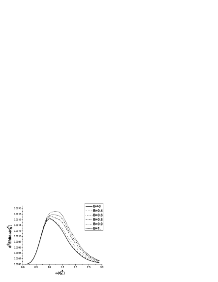
Figure 2: Hawking spectrum of a $6D$ bulk scalar as a function of brane tension. $B$ changes from $B=1$ (tensionless brane) to $B=0$ (deficit angle equal to $2\pi$).

We should stress that our method of calculating the Hawking radiance by bulk mode expansion is completely equivalent to first performing the Kaluza-Klein reduction of bulk scalar perturbations and then expanding in the $SO(3)$ representations reflecting the black hole horizon symmetry. This way of thinking about organizing the calculation is particularly useful in computing the higher spin emissions, which we turn to next.

The calculation of Hawking radiance for bulk vectors and tensors goes similarly to the one for scalars, with the exception that one has to properly account for the helicity multiplets. Namely, in the case of massless $4D$ vectors and tensors, gauge symmetries ensure that the only propagating modes are, in the traceless-transverse Lorentz and de Donder gauge, respectively, the helicity-1 and helicity-2 modes, like the usual Maxwell and Einstein fields. However, in the higher-dimensional case they are accompanied by the Kaluza-Klein towers of massive modes. These have less gauge symmetry and hence contain more propagating degrees of freedom, including extra scalars, and scalars and vectors in the bulk vector and bulk tensor cases, respectively, which span the full massive $4D$ vector and tensor multiplets grw .

Now, in computing the Hawking radiance from small hot black holes we can neglect the $4D$ mass for most of these modes since they lie well below the cutoff while the black hole’s temperature is close to it, but these extra modes still carry away the black hole energy. Thus we must take them into account. A simple way to do this is to dimensionally decompose the relevant representations into $4D$ tensors, vectors and scalars, as has been done in 5 ; 6 ; 7 , with respect to the transverse space to the direction of motion. In practice, this means counting the tensor representations over the deformed transverse $S^{4}$ in Eq. (1), because by the axial symmetries of the problem the energy will flow radially outward from the hole. Thus the radial direction and the time can be factored out. Then, by going to the unitary gauge, we will find that each degree of freedom obeys a field equation similar to the one for scalars. Working out the details, one can show that the master equation for the radial part of a higher dimensional gauge boson or graviton field (see 5 ; 6 ; 7 ) propagating in the background of the black hole (1) is

$$\frac{d^{2}\Psi}{dr^{*2}}+(\omega^{2}-V(r))\Psi=0\,,$$ (16)

where

$$V(r)=F(\frac{\eta}{r^{2}}+\frac{2}{r^{2}}+\frac{4(1-p^{2})}{r^{5}})\,.$$ (17)

The constant p is given by $0$ for scalars and tensor gravitons, $2$ for gravi-vectors, $1/2$ for gauge vectors and $3/2$ for scalar reductions of bulk vectors. For example, as a quick check we can see that setting $p=0$ and $\Psi=r^{2}R$ in (16) we readily recover Eq. (6).) One further finds that for the higher spin fields the angular quantum number $L$ is restricted by the spin, so that its range is 5 ; 6 ; 7 ; 8 :

$$L=\left\{\begin{array}[]{ll}0,1...&\mbox{for scalar perturbation}\,,\\ 1,2...&\mbox{for vector perturbation}\,,\\ 2,3...&\mbox{for tensor perturbation}\,.\end{array}\right.$$

Finally for gravitational scalar perturbations one finds 5 ; 7

$$V=F\frac{Q(r)}{16r^{2}H(r)^{2}}\,,$$ (18)

with

$$Q(r) = 6400r^{-9}+1920(\eta-4)r^{-6}-1920(\eta-4)r^{-3}$$

$$+ 16(\eta-4)^{3}+96(\eta-4)\,,$$

$$H(r) = (\eta-4)+10r^{-3}\,.$$ (19)

What then remains is to determine the eigenvalues $\eta$ and the and the number of states for each fixed $\eta$. This number depends on the helicity, and for the scalars the degeneracy $N^{\rm scal}_{L,m}$ is the same as in Eq. (Evaporation of a black hole off of a tense brane). For the vectors, one needs to account properly for gauge fixing when counting the solutions of the angular equation of motion 8 . In the end the vector degeneracies depend only on the helicity and not on how it is lifted into the bulk, yielding

$$m=0 : N^{\rm vec}_{L,m}=\frac{L(3L+5)}{2}$$ (20)

$$m\neq 0 : N^{\rm vec}_{L,m}=3(L-m+2)(L-m+1)\,.$$

In the case of transverse-traceless tensors, the problem of solving the gauge fixed angular equation is more difficult. To determine the degeneracies, we need to solve $\nabla^{\alpha}\nabla_{\alpha}T_{\mu\nu}=0$ satisfying gauge conditions $\nabla^{\mu}T_{\mu\nu}=0$ and $T^{\mu}{}_{\mu}=0$, where $\nabla^{\alpha}\nabla_{\alpha}$ is the covariant Laplacian on $S^{4}$, and all the indices $\alpha,\mu,\nu$ run over the deformed transverse sphere of Eq. (1), as we noted above. Now, below some high (angular!) momentum cutoff, the total number of states is the same as in the spherically symmetric limit, computed in RO and summarized in the Table I of that paper. The only effect of broken spherical symmetry is splitting between some of the levels that were degenerate on $S^{4}$. Then for $L\geq|m|\geq 2$ the transverse-traceless tensor can be viewed as an array of five scalars, and we can simply count up the number of states for each of them and add them up. This yields $N^{\rm ten}_{L,m}=5(L-m+2)(L-m+1)$ for $L\geq|m|\geq 2$. What remains then is to account for the states with $m=0,1$. We can do this by taking the total number of states from RO , subtracting all the states with $|m|\geq 2$, whose number we just worked out, and recalling that the number of states with $L=2,m=0$ is really the number of independent $s$-wave modes in the full $6D$ graviton multiplet at some fixed mass level. Since the number of independent propagating modes of a $6D$ graviton is nine, we must fix $N(L=2,m=0)=9$. This then uniquely determines the degeneracies to be

$$m=0 : N^{\rm ten}_{L,m}=\frac{(L-1)(5L+8)}{2}\,,$$

$$m=1 : N^{\rm ten}_{L,m}=(L-1)(5L+6)\,,$$

$$m\geq 2 : N^{\rm ten}_{L,m}=5(L-m+2)(L-m+1)\,.$$ (21)

Then using the same asymptotic form of the radial wavefunctions as for the scalars (Evaporation of a black hole off of a tense brane) and defining the absorption ratio for each helicity as $|\tilde{A^{j}}_{L,m}|^{2}=1-\left({A^{(\infty)}_{out}}/{A^{(\infty)}_{in}}\right)^{2}$, where $j$ labels the helicity, we can write the Hawking radiance spectrum for each mode as

$$\frac{d^{2}E}{dtd\omega}=\sum_{L,m}\frac{\omega}{e^{\omega/T_{h}}-1}\frac{1}{2\pi}\sum_{j}N^{j}_{L,m}|\tilde{A}^{j}_{L,m}|^{2}\,.$$ (22)

For vectors, $j$ takes values for scalar and Lorentz vector, whereas for tensors it runs over all scalars, vectors and transverse-traceless tensor modes with fixed quantum numbers $L$ and $m$. This is the total power emitted in the frequency band $d\omega$. For the power emitted per degree of freedom, we ought to divide the result (22) by four for a gauge boson and by nine for graviton, since $6D$ bulk vectors and tensors have $4$ and $9$ degrees of freedom, respectively, as we have discussed above.

We have computed the power (22) numerically for the relevant vector and tensor modes. In Fig. 3 we show the dependence of the Hawking radiation spectrum for bulk vectors on the brane tension, while in Fig. 4 we display the dependence of the radiance on tension for the graviton field. Finally, for completeness, in Fig. 5 we show the Hawking spectrum of brane-localized fields, which for a fixed horizon size $r_{h}$ does not depend on the tension. Of course, the horizon size $r_{h}$ depends on the tension as given in Eq. (2). In order to get the power per channel from the total power displayed in Fig. (5), we need to halve the fermion and gauge boson distribution.

Figure 3: Hawking radiation spectrum for a bulk gauge boson as a function of the brane tension. $B$ changes from $B=1$ (tensionless brane) to $B=0$ (deficit angle equal to $2\pi$).

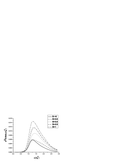
Figure 4: Hawking radiation spectrum for a bulk tensor as a function of the brane tension. Again, $B$ changes from $B=1$ (tensionless brane) to $B=0$ (deficit angle equal to $2\pi$).

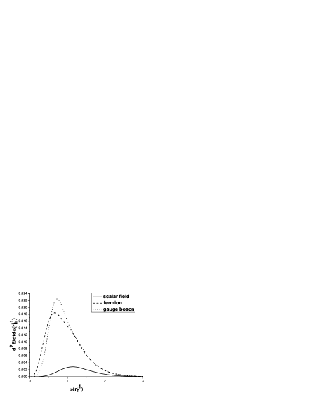
Figure 5: Hawking radiation of brane localized fields: a scalar, a fermion and a vector gauge boson. For fixed horizon size they are not affected by the finite tension of the brane.

In sum, collider searches for black holes may be an exciting and interesting source of information about extra dimensions, complementing possible astrophysical tests (for recent exploration of those, see ruth ). In this note we have explored the Hawking decay channels for a recently constructed exact black hole localized on a $3$-brane KK . We see that brane tension may alter significantly the power output of small black holes located on the brane. While for the non-rotating black holes the dominant channels are still the brane-localized modes, in realistic models with split fermions as in AS , the gauge boson contribution to black hole radiance may be significant. Since they need to be in the bulk to communicate between different (families of) quarks and leptons, the gauge boson emissions may be a sensitive probe of deficit angle and therefore brane tension. Specifically, we see that the power emitted in the bulk diminishes as the tension increases. This may appear slightly odd at first sight since increasing the tension for fixed $M_{4}$ strengthens effective bulk gravity KK . However, when the horizon $r_{h}$ is held fixed, this comes about because the gravitational potential barrier depends on the eigenvalue $\eta$, which as seen in Fig. (1) increases as the parameter $B$ decreases, and tension increases. Therefore the potential barrier grows reducing the rate of energy loss. Similarly, at fixed black hole mass increasing the tension would simultaneously increase the horizon size, lowering the temperature and increasing the black hole entropy. Hence in this case a black hole will also radiate away its mass more slowly. If we ever produce small black holes at the LHC, the total Hawking radiance will be a sum of the power emitting along the brane and off of it. In simple toy models the emission into the bulk would be subleading because of the $s$-wave dominance, leading to essentially negligible bulk effects. However in more realistic models with split fermions and gauge fields in the bulk, the balance between contributions from the brane and bulk modes may end up being significantly tilted in favor of the increasing number of bulk modes. While the precise details of course would be very model dependent, in such cases the off the wall contributions may be significant, and so the effects we have described here may play an important role, warranting a careful and detailed examination of Hawking radiation losses.

Acknowledgment

NK and GDS thank the Galileo Galilei Institute, Florence, for kind hospitality in the course of this work. GDS also thanks the Beecroft Institute for Particle Astrophysics and Cosmology and The Queen’s College, Oxford for hospitality and support. The work of NK was supported in part by the DOE Grant DE-FG03-91ER40674, in part by the NSF Grant PHY-0332258 and in part by a Research Innovation Award from the Research Corporation. The work of GDS was supported in part by the John Simon Guggenheim Memorial Foundation.

References

- (1) N. Arkani-Hamed, S. Dimopoulos and G. R. Dvali, Phys. Lett. B 429, 263 (1998); I. Antoniadis, N. Arkani-Hamed, S. Dimopoulos and G. R. Dvali, Phys. Lett. B 436, 257 (1998).
- (2) T. Banks and W. Fischler, arXiv:hep-th/9906038; P. C. Argyres, S. Dimopoulos and J. March-Russell, Phys. Lett. B 441, 96 (1998); S. Dimopoulos and G. Landsberg, Phys. Rev. Lett. 87, 161602 (2001); S. B. Giddings and S. D. Thomas, Phys. Rev. D 65, 056010 (2002).
- (3) R. Emparan, G. T. Horowitz and R. C. Myers, Phys. Rev. Lett. 85, 499 (2000).
- (4) J. L. Feng and A. D. Shapere, Phys. Rev. Lett. 88, 021303 (2002); D. Stojkovic and G. D. Starkman and D. C. Dai, Phys. Rev. Lett. 96, 041303 (2006).
- (5) N. Arkani-Hamed and M. Schmaltz, Phys. Rev. D 61, 033005 (2000); N. Arkani-Hamed, Y. Grossman and M. Schmaltz, Phys. Rev. D 61, 115004 (2000); T. Han, G. D. Kribs and B. McElrath, Phys. Rev. Lett. 90, 031601 (2003); D. C. Dai, G. D. Starkman and D. Stojkovic, Phys. Rev. D 73, 104037 (2006); D. Stojkovic, F. C. Adams and G. D. Starkman, Int. J. Mod. Phys. D 14, 2293 (2005).
- (6) N. Kaloper and D. Kiley, JHEP 0603, 077 (2006).
- (7) P. D. D’Eath and P. N. Payne, Phys. Rev. D 46, 658 (1992); Phys. Rev. D 46, 675 (1992); Phys. Rev. D 46, 694 (1992).
- (8) D. M. Eardley and S. B. Giddings, Phys. Rev. D 66, 044011 (2002).
- (9) J. W. Chen, M. A. Luty and E. Ponton, JHEP 0009, 012 (2000); Y. Aghababaie et al., JHEP 0309, 037 (2003); see also N. Arkani-Hamed, L. J. Hall, D. R. Smith and N. Weiner, Phys. Rev. D 62, 105002 (2000).
- (10) E. G. Adelberger, B. R. Heckel and A. E. Nelson, Ann. Rev. Nucl. Part. Sci. 53, 77 (2003); for most recent bounds, see D. J. Kapner, T. S. Cook, E. G. Adelberger, J. H. Gundlach, B. R. Heckel, C. D. Hoyle and H. E. Swanson, arXiv:hep-ph/0611184.
- (11) T. Vachaspati, D. Stojkovic and L. M. Krauss, arXiv:gr-qc/0609024.
- (12) C. M. Harris and P. Kanti, JHEP 0310, 014 (2003); P. Kanti and J. March-Russell, Phys. Rev. D 66, 024023 (2002); Phys. Rev. D 67, 104019 (2003); J. y. Shen, B. Wang and R. K. Su, Phys. Rev. D 74, 044036 (2006); D. Ida, K. y. Oda and S. C. Park, Phys. Rev. D 67, 064025 (2003)
- (13) W. H. Press, S. A. Teukolsky, W. T. Vetterling and B. P. Flannery, Numerical Recipes in C: The art of scientific computing, Cambridge University Press.
- (14) D. Stojkovic, Phys. Rev. Lett. 94, 011603 (2005); V. P. Frolov and D. Stojkovic, Phys. Rev. Lett. 89, 151302 (2002); Phys. Rev. D 66, 084002 (2002).
- (15) G. F. Giudice, R. Rattazzi and J. D. Wells, Nucl. Phys. B 544, 3 (1999).
- (16) H. Kodama and A. Ishibashi, Prog. Theor. Phys. 110, 701 (2003); Prog. Theor. Phys. 110, 901 (2003); Prog. Theor. Phys. 111, 29 (2004).
- (17) L. C. B. Crispino, A. Higuchi and G. E. A. Matsas, Phys. Rev. D 63, 124008 (2001).
- (18) V. Cardoso, M. Cavaglia and L. Gualtieri, JHEP 0602, 021 (2006).
- (19) R. Camporesi and A. Higuchi, J. Geom. Phys. 15 57 (1994).
- (20) M. A. Rubin and C. R. Ordonez, J. Math. Phys. 26, 65 (1985).
- (21) R. Gregory, R. Whisker, K. Beckwith and C. Done, JCAP 0410, 013 (2004); S. Creek, R. Gregory, P. Kanti and B. Mistry, Class. Quant. Grav. 23, 6633 (2006).