Theta Vacua and Boundary Conditions of the Schwinger-Dyson Equations

Quantum field theories and Matrix models have a far richer solution set than is normally considered, due to the many boundary conditions which must be set to specify a solution of the Schwinger-Dyson equations. The complete set of solutions of these equations is obtained by generalizing the path integral to include sums over various inequivalent contours of integration in the complex plane. We discuss the importance of these exotic solutions. While naively the complex contours seem perverse, they are relevant to the study of theta vacua and critical phenomena. Furthermore, it can be shown that within certain phases of many theories, the physical vacuum does not correspond to an integration over a real contour. We discuss the solution set for the special case of one component zero dimensional scalar field theories, and make remarks about matrix models and higher dimensional field theories that will be developed in more detail elsewhere. Even the zero dimensional examples have much structure, and show some analogues of phenomena which are usually attributed to the effects of taking a thermodynamic limit.

bla

MIT-CTP-2582

PUPT-1670

I Introduction

This paper is a consequence of our ongoing study of a new numerical approach to quantum field theory, known as the Source Galerkin [1, 2, 3] technique. This method is based on systematically approximating the functional differential equations, or Schwinger-Dyson equations, satisfied by the generating functional in quantum field theory, while controlling the error with a weighted averaging procedure. While exploring this method, it came to our attention that it is necessary to carefully analyze the boundary conditions imposed on these equations.

Here, we address this problem from a formal rather than a numerical point of view. For any theory with a large but finite number of degrees of freedom, there are a very large number of “theta” parameters characterizing solutions of the Euclidean Schwinger-Dyson equations, which are the quantum mechanical version of the equations of motion. Only one point in this parameter space corresponds to the usual path integral . It is therefore tempting to discard all the other solutions as unphysical. However, we shall argue that under many conditions the exotic solutions are physical. Symmetry breaking vacua provide the simplest examples of a situation in which exotic solutions are physical. Furthermore, critical phenomena have a natural interpretation in terms of the behavior of the full solution set in the thermodynamic limit. In this limit the solutions associated with many different boundary conditions coalesce. For other boundary conditions, the limit does not exist. Which boundary conditions have a thermodynamic limit and which ones coalesce depends on the theory’s parameters in a manner which determines the phase diagram and the critical exponents.

In section II we discuss the boundary conditions of some simple zero dimensional scalar theories. In addition to the usual integral solution of the Schwinger-Dyson equations, there are exotic solutions which are obtained from sums over various inequivalent complex contours of integration. Zero dimensional theories have many phases, all of which are continuously related. For symmetric actions these include symmetry breaking solutions.

In section III, we describe the boundary conditions of the Schwinger-Dyson equations for a general theory with a finite number of degrees of freedom. For a Euclidean field theory on a finite lattice without a boundary, the complete set of solutions may be obtained from different complex integral representations and have a simple correspondence to the classical solutions of the theory. The exotic solutions may be thought of as generalized lattice theta vacua. There is a still larger class of solutions which may be obtained on a lattice with a boundary, at which the Schwinger-Dyson equations may be modified. In the integral representation of the solution, the measure for fields at the boundary is essentially arbitrary, and may be set by surface terms in the action or by wave functions. However we will confine our discussion to generating functionals in the vacuum sector. These may be obtained on a periodic lattice, for which the exotic contours provide a complete set of boundary conditions. In the thermodynamic limit the real path integration with surface terms in the action gives some but not all of the solutions found using complex contours for a periodic lattice. There are compelling reasons to consider solutions represented by exotic contours, of which we list a few below. One reason is that certain aspects of critical phenomena are very naturally related to the behavior of the full set of solutions, including those which are unphysical, in the thermodynamic limit. The full solution set may only by obtained by allowing complex contours. Furthermore solutions corresponding to false vacua may be of physical interest but are not obtainable from the integration over real fields. In the case of matrix models it is essential to consider exotic contours to obtain even certain physical solutions with a real double scaling limit. This is true even when the matrix potential is bounded below for real eigenvalues. In this case there is no analogue of a spatial boundary at which the measure may be arbitrary. There are often many physical solutions having a real double scaling limit. One can obtain some of these solutions from the integration over real eigenvalues by making global perturbations of the action which are removed after taking the $N\rightarrow\infty$ or double scaling limit. However there are also examples of solutions which can not be found this way[4][5][6]. On the other hand, the complete set of exotic contours does yield the full solution set[5][6][7]. There are situations in which the boundary conditions associated with a real solution in the double scaling limit are extremely unusual[5][6].

In section IV, we discuss phenomena which occur in the thermodynamic limit in the context of the Euclidean Schwinger-Dyson equations. In particular, we discuss the coalescence of solutions associated with different boundary conditions, and the absence of a thermodynamic limit for other boundary conditions. In some cases one can explicitly see how the solution set collapses, as in certain large $N$ matrix models. The solutions which survive in this limit do not necessarily coalesce with a solution associated with the integral over real fields, and sometimes the integral over real fields itself does not have a thermodynamic limit. In this paper we will not explicitly demonstrate the collapse of the solution set. Instead we will assume the collapse and show that it leads to several expected phenomena, such as the appearance of phase boundaries in the thermodynamic limit due to the accumulation of Lee-Yang zeroes. Critical exponents are determined by the manner in which the solution set collapses. We give a simple zero dimensional analogy in which tuning a coupling constant to zero shrinks the solution set and causes Lee-Yang zeroes to accumulate. Setting the coupling constant to zero in this example is analogous to taking the thermodynamic limit. We also show that the collapse of the solution set induces another set of well known equations which we will refer to as the Schwinger action principle;

$${\partial\over\partial g}Z=<{\partial S\over\partial g}>Z$$ (1)

Here $g$ is a parameter of the the action $S$, and $Z$ is the partition function. If one only considers the usual solution of the Schwinger Dyson equation corresponding to the integral over real eigenvalues in a matrix model, or real fields in a field theory on a periodic lattice, then the action principle is obviously obeyed. However, as soon as one considers all of the solutions of the Schwinger-Dyson equations, it is no longer obvious that the action principle should be satisfied. For a finite system the action principle is independent of the Schwinger-Dyson equations. It is possible to satisfy the Schwinger-Dyson equations while violating the action principle. Since the solution set does not necessarily collapse to the usual integral solution, it is nontrivial to show that the action principle follows from the Schwinger-Dyson equations in the thermodynamic limit.

In section V we discuss the effect of the collapse of the solution set on the form of the effective potential. For a finite number of degrees of freedom, there are an infinity of effective potentials, each of which has only single extremum. In the thermodynamic limit, it is possible to have a single effective potential with multiple extrema.

II Boundary conditions of Schwinger-Dyson equations

When there is no spatial boundary, the set of boundary conditions of the Schwinger-Dyson equations is determined by the behavior of the action at asymptotic values of the fields. The reasons for this will become clear shortly. For many theories a potential term dominates the action at large fields, and we will begin by considering a theory with only a potential term. Let us find the space of solutions for a polynomial action with one degree of freedom,

$$S=\sum_{l=1}^{n}{1\over l}g_{l}\phi^{l}$$ (2)

The generating function $Z(J)$ of disconnected Green’s functions satisfies the Schwinger-Dyson equation:

$$\sum_{l=1}^{n}(g_{l}{\partial^{l-1}\over\partial J^{l-1}}-J)Z(J)=0$$ (3)

This is a linear differential equation of order $n-1$, and has an $n-1$ parameter set of solutions. One parameter corresponds to a trivial normalization factor, so there is an $n-2$ parameter set of solutions with different Green’s functions. There is a complete basis set of solutions with the integral representation

$$Z(J)=\int_{\Gamma}\,d\phi{\displaystyle{e^{-S(\phi)+J\phi}}}$$ (4)

where $\Gamma$ is a complex path such that

$$\int_{\Gamma}\,d\phi{\partial\over\partial\phi}{\displaystyle{e^{-S(\phi)+J\phi}}}=0$$ (5)

or

$$\left.{\displaystyle{e^{-S(\phi)+J\phi}}}\right|_{\partial\Gamma}=0.$$ (6)

The paths for which this is true is determined by the order of the polynomial potential. We require $Re(g_{n}\phi^{n})\rightarrow+\infty$ as $|\phi|\rightarrow\infty$, giving $n$ domains in which the contour can run off to infinity (fig.1). One can then write down $n-1$ independent contours which comprise a basis set. The contours may not be deformed into one another since $e^{-S}$ is not analytic at $|\phi|\rightarrow\infty$. For $S={1\over 4}g\phi^{4}+...$ with $g$ real, one choice of independent contours is

$$\Gamma^{+}=[-\infty,0]+[0,+i\infty]$$ (7)

(8)

$$\Gamma^{0}=[-\infty,0]+[0,+\infty]$$ (9)

(10)

$$\Gamma^{-}=[-\infty,0]+[0,-i\infty]$$ (11)

with which we associate the generating functions $Z^{+},Z^{0}$ and $Z^{-}$. As a matter of definition, we will say that solutions at different values of $g$ are in the same phase if they are related by the the Schwinger action principle,

$$({\partial\over\partial g}+{1\over 4}{\partial^{4}\over\partial J^{4}})Z=0.$$ (12)

For the example above, a general solution of the Schwinger-Dyson equations is of the form $Z=aZ^{+}+bZ^{0}+cZ^{-}$ where $a$, $b$ and $c$ may be arbitrary functions of $g$. The solutions $Z^{+}$, $Z^{0}$ and $Z^{-}$ separately satisfy the action principle. Therefore the action principle is satisfied if $a$,$b$ and $c$ are independent of $g$. A phase is labeled by the ratios of these three constants. However as $Re(g)$ becomes negative, the contours $\Gamma^{+},\Gamma^{0}$ and $\Gamma^{-}$ are no longer convergent. For $g$ real and positive, there are domains swept out by contours equivalent to $\Gamma^{+},\Gamma^{0}$ and $\Gamma^{-}$. As one rotates the phase of $g$, these domains also rotate to maintain convergence. So to be more precise the action principle is satisfied if for infinitesimal variations of $g$ there is a choice of contours which is held fixed. If one makes large changes in $g$, it may be necessary to change the contour. Thus the statement that two solutions are in the same phase if they are related by the action principle makes sense only locally in the space of coupling constants. A large loop in coupling constant space can go around a phase boundary and onto another Riemann sheet, thus changing the boundary condition. In the above example there is a phase boundary at $g=0$, and a $2\pi$ rotation of $g$ forces a ${\pi\over 2}$ rotation of the contour to maintain convergence. Note that in zero dimensions the Schwinger action principle is a very arbitrary way to define a phase. One could have required the generating function within a given phase to satisfy any other set of first order differential equations in the couplings. As we shall see later, the action principle is a consequence of the Schwinger-Dyson equations in the thermodynamic limit .

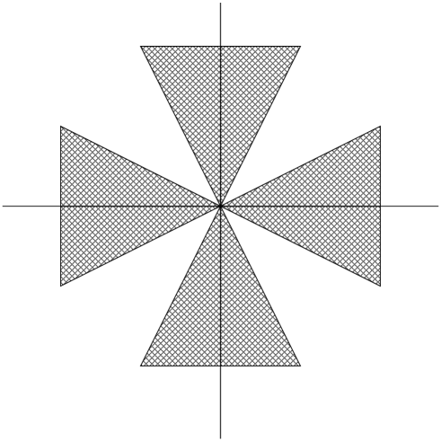
FIG. 1.: The shaded area is the region of the complex $\phi$ plane defined by $\cos(4\theta)>0$, where $\theta$ is the argument of $\phi$. Any path starting and ending at infinity within one of these four domains corresponds to a particular solution for the zero dimensional $\phi^{4}$ theory

For the example of the action $S={g\over 4}\phi^{4}+{1\over 2}\mu\phi^{2}$ the exact disconnected Green’s functions (see Appendix I) satisfying both the Schwinger-Dyson equations and the action principle are given by;

$$G_{2n}=\mu^{-n}(2n-1)!!t^{n}{U(n,t)+(-1)^{n}\rho U(n,-t)\over U(0,t)+\rho U(n,-t)}$$ (13)

and

$$G_{2n+1}=\mu^{-n-{1\over 2}}{2n!!\over n!}(-t)^{n}{V(n+{1\over 2},t)\over V({1\over 2},t)}\alpha{t^{1\over 2}e^{t^{2}\over 4}\over U(0,t)+\rho U(0,-t)}$$ (14)

where $t=\sqrt{\mu^{2}\over 2g}$, and $U(a,t)$ and $V(a,t)$ are parabolic cylinder functions defined in appendix I. The parameters $\alpha$ and $\rho$ depend on the ratios of the coefficients, $a$, $b$ and $c$, of the independent contours. By requiring Green’s functions to be real, or that $a$ be real and $b=c^{*}$, one is still left with many exotic solutions. These are labeled by the two real parameters $\alpha$ and $\rho$. Solutions with $\alpha\neq 0$ break the $\phi\rightarrow-\phi$ symmetry of the action. Such solutions exist because the contours $\Gamma^{+}$ and $\Gamma^{-}$ break the symmetry.

Since reality is not much of a constraint on the solution set, it might be tempting to require positivity of even Green’s functions as well. This is a much stronger constraint, since only the solution corresponding to the real contour is manifestly positive. For a general boundary condition, one must do some work to ascertain positivity. However, it does not make sense to impose positivity before taking a thermodynamic limit, because the conditions for positivity may change in this limit. Our approach to the selection of boundary conditions will be to let the thermodynamic limit do most of the selection for us. We shall argue later that the solution set collapses in the thermodynamic limit. By this we mean that the solutions associated with certain continuous classes of boundary conditions coalesce, while other boundary conditions lead to no thermodynamic limit. The surviving solutions may then include some which violate reflection positivity (for Euclidean Schwinger-Dyson equations), and these may be discarded by hand. Note that sometimes complex solutions describe false vacua and are of physical interest.

One might also try to constrain the solution set by requiring that the weak coupling limit smoothly approach the free field solution. This would mean that $Z$ should have the formal representation

$$Z(g,J)=e^{{g\over 4}\partial_{J}^{4}}Z(0,J)$$ (15)

This is a very strong constraint reflecting the fact that the Schwinger-Dyson equation becomes first order at $g=0$. For the zero dimensional $\phi^{4}$ theory the equation is $(\mu\partial_{J}-J)Z=0$ and, consequently, has only one solution up to a normalization. However, this constraint is ill defined if there are any phase boundaries in $g$. In our zero dimensional example there is a branch point at $g=0$, so the result of taking a weak coupling limit depends on the path. One could take $g\rightarrow 0$ with the phase of $g$ fixed. There is no physical reason why the partition function should have a free field limit as $g\rightarrow 0$. In the symmetry breaking phase of a $g\phi^{4}$ theory, the Green’s functions are singular at $g=0$. For instance, the one point function at weak coupling is $<\phi>=\sqrt{-{\mu\over g}}$. For our zero dimensional example, the requirement of a free field $g\rightarrow 0$ limit with $\mu<0$ would yield the symmetric boundary condition corresponding to an integral over the imaginary axis.

It is enlightening to consider the weak coupling limit of the full set of solutions of the zero dimensional $\phi^{4}$ theory. There are some solutions to which the effective potential in the loop expansion is asymptotic. These correspond to sums over contours which pass through a single dominant saddle point. At each order in the loop expansion the effective potential has three extrema corresponding to each saddle point and a different class of boundary conditions . Among these are symmetry breaking solutions with the asymptotic expansion for the one point function given by

$$<\phi>=\sqrt{-{\mu\over g}}(1+O(g)+\dots)$$ (16)

$Z^{+}$ is one example of a solution with this expansion. Another example which is real is $Z^{+}+Z^{-}$ for $g>0$ and $\mu<0$. One can explicitly show that such a boundary condition leads to the symmetry breaking phase of a $Tr\phi^{4}$ matrix model[5][6][7]. It seems natural to conjecture that some generalization of such a boundary condition also corresponds to the symmetry breaking phase of a $\phi^{4}$ field theory.

There is yet another class of solutions of the zero dimensional $\phi^{4}$ theory which does not correspond to the loop expansion. These arise when the contours cross degenerate dominant saddle points. These solutions are linear combinations of the ones associated with the loop expansion. Some of these are extremely singular at weak coupling. For instance for $\mu>0$ and $g>0$, the solution $Z=Z^{+}+Z^{-}$ has a one point function with the expansion

$$<\phi>=\sqrt{{-\mu\over g}}e^{+{\mu^{2}\over 4g}}(1+\dots)$$ (17)

This is also the expansion for a similar solution in the case $\mu<0$, but the boundary condition is different, with contours rotated by $\pi\over 2$. The essential singularity $e^{+\mu^{2}\over 4g}$ arises because $<\phi>={\partial_{J}Z\over Z}$, and the contribution of the two degenerate dominant saddle points at $\phi=\sqrt{{-\mu\over g}}$ cancels in the denominator but not in the numerator. In one matrix models it is easy to see that boundary conditions of this singular type do not have a thermodynamic limit [5][6]. However at this point of our discussion we already have some evidence that some the other exotic boundary certainly may be physical, the simplest example being that of the symmetry breaking solutions associated with the loop expansion.

Our interest in $\phi^{4}$ theory is primarily as a toy model. The same analysis may be applied to obtain the solution set for non-polynomial actions, in which the order of the Schwinger-Dyson equations is not always obvious. A simple example is given by the loop equation of one plaquette QED, which is defined by the action $S=-\beta cos\phi$. The condition that $e^{-S}$ vanishes as $|\phi|\rightarrow\infty$ restricts the domain of integration to satisfy $Re(\beta cos\phi)\rightarrow+\infty$ asymptotically. For $\beta$ real and positive, one choice of inequivalent contours which satisfy this requirement is given by

$$\Gamma_{1}=[-i\infty,+i\infty]$$ (18)

and

$$\Gamma_{2}=[-i\infty,0]+[0,2\pi]+[2\pi,2\pi+i\infty]$$ (19)

to which we associate the partition functions $Z_{1}$ and $Z_{2}$. Due to the periodicity in $Re(\phi)$, it is easy to see that any other allowed contour may be written as linear combination of these two. The difference between $Z_{1}$ and $Z_{2}$ is just the usual integral defined on the compact interval $[0,2\pi]$. Note that only this solution manifestly satisfies the condition that $|<e^{i\phi}>|<1$. However along the lines of our previous arguments, we will not impose such conditions before taking a thermodynamic limit.

Given that there are two independent contours, we expect that the Schwinger-Dyson equations should be second order. In this case, it is easy to construct the equations even though the action is not polynomial. By coupling sources $J$ and $\bar{J}$ to the loop variables $e^{i\phi}$ and $e^{-i\phi}$ one obtains the Schwinger-Dyson equations

$$[\beta(\partial_{J}-\partial_{\bar{J}})-2(J\partial_{J}-{\bar{J}}\partial_{\bar{J}})]Z(J,{\bar{J}})=0$$ (20)

and the constraint

$$\partial_{J}\partial_{\bar{J}}Z(J,{\bar{J}})=Z.$$ (21)

These equations may be rewritten in the form

$${\beta-2J\over\beta-2{\bar{J}}}\partial_{J}^{2}Z=Z$$ (22)

and

$$\partial_{\bar{J}}Z={\beta-2J\over\beta-2{\bar{J}}}\partial_{J}Z$$ (23)

which, accounting for the normalization of $Z$, has a one dimensional space of solutions characterized by the above integral representations. Of course, in contrast to a theory with a local order parameter, one can not hope to learn very much about the phases of a gauge theory from a zero dimensional (one plaquette) model. Note that lattice gauge theories are examples of theories in which the large field behavior of action, and therefore the choice of boundary conditions, is not controlled by independently variable local terms, due to the constraints among the plaquettes. However the one plaquette model does illustrate something which is true generally. The “exotic” solutions of the loop equations for a gauge theory correspond to certain complexifications of the gauge group. Similarly, in hermitian matrix models the exotic solutions correspond to certain complexifications of the eigenvalues in the matrix integral, and in this case it can be proven that some of the exotic solutions are “physical” for certain values of the couplings, meaning that a real double scaling limit exists.

III From Zero to Higher Dimension

For theories in which independently variable local terms dominate the large field behavior of the action, it is straightforward to represent the higher dimensional theory in terms of a zero dimensional theory. Such representations are the starting point for both the strong coupling and mean field expansions. For example, consider the lattice Schwinger-Dyson equations of an interacting scalar field with action $S={1\over 2}\sum_{x,y}H_{x,y}\phi_{x}\phi_{y}+\sum_{x}V(\phi_{x})$:

$$(\sum_{y}H_{x,y}{\partial\over\partial J_{y}}+V^{\prime}({\partial\over\partial J_{x}})-J_{x})Z[J]=0.$$ (24)

A formal solution corresponding to the strong coupling expansion is given by

$$Z[J]=e^{{1\over 2}\sum_{x,y}{\partial\over\partial J_{x}}H_{x,y}{\partial\over\partial J_{y}}}\prod_{w}Z_{0}(J_{w})$$ (25)

where $Z_{0}(J)$ is any solution of the zero dimensional Schwinger-Dyson equation

$$(V^{\prime}({\partial\over\partial J})-J)Z_{0}(J)=0.$$ (26)

The solution also may be written as

$$Z[J]=\int\prod_{x}d\rho_{x}e^{-{1\over 2}\sum_{x,y}H^{-1}_{x,y}\rho_{x}\rho_{y}}\prod_{x}Z_{0}(J_{x}+\rho_{x}).$$ (27)

This may be thought of as a stochastically driven zero dimensional theory. A saddle point expansion in the auxiliary variable $\rho$ yields a mean field expansion. We shall not make any use of these expansions here, but just mention them to illustrate the structure of the solution set in non-zero dimensions. In both the representations there is a product over zero dimensional solutions at each lattice site. It is not necessary to use the same integration contour at every lattice site, even if lattice symmetry is required of the solution. A sum over translations and rotations of solutions with inhomogeneous boundary conditions yields a solution which satisfies the lattice symmetries, and yet can not always be written in terms of an integral over a product of equivalent measures at each lattice site (fig.2). In a future publication[6] we show that there are matrix model solutions with this type of boundary condition. In this case the lattice site is replaced with an eigenvalue label, and the integral representation does not involve a single measure for each eigenvalue[6]. This means that the solution is not of the form,

$$Z=\prod_{n}\left(\sum_{i}c_{i}\int_{\Gamma_{i}}d\Lambda_{n}\right)\Delta^{2}[\Lambda]e^{-N\sum_{m}V(\Lambda_{m})}.$$ (28)

where $\Lambda_{n}$ are the eigenvalues, and $\Delta[\Lambda]$ is the Vandermonde determinant. If we consider only solutions of this form, which involve products of equivalent measures over the lattice sites, then the space of boundary conditions on a periodic lattice is the same as that of the zero dimensional theory.

FIG. 2.: A pictorial representation of translationally invariant solutions on a two site lattice. (a) is a product over equivalent measures at each lattice site. (b) may not be written as a product over equivalent measures at each site.

Note, however, that there is a class of theories for which there is no simple relation between the space of boundary conditions in a zero dimensional theory and a subspace of the boundary conditions on a periodic lattice. This class consists of theories in which the action at large values of the fields is not dominated by independently variable local terms. We have stated that gauge theories fall in this class. Another example of a theory in this class is the XY model, with lattice action

$$S=-{1\over 2}H_{x,y}cos(\theta_{x}-\theta_{y}).$$ (29)

For such theories it is usually much harder to de-numerate the boundary conditions of the Schwinger-Dyson equations, although there is a partial classification based on generalized lattice theta vacua which we discuss shortly. It seems likely that there is an equivalence or at least a large overlap between theories without a local order parameter, and theories for which the boundary conditions are not determined by independent local terms. Note that for a theory in which local terms control the boundary conditions, such as the $\phi^{4}$ theory, the behavior of the local order parameter $<\phi>$ is determined by the choice of these boundary conditions. If in the thermodynamic limit the solution set collapses, then certain boundary conditions and therefore certain values of the order parameter are selected.

To argue that the exotic solutions involving complexified fields may in fact be physical, we have so far given the example of symmetry breaking. We will now try to make our arguments more concrete. While the exotic solutions may appear very strange, many of them are actually familiar. For example, there is a simple relation between conventional theta vacua and exotic solutions with complexified fields, which we demonstrate below. For some simple cases it can be shown that a complete set of solutions of the Schwinger-Dyson equations may be generated from the complete set of classical solutions, both real and complex. This relation may be made explicit through the Borel re-summation of perturbative expansions about the classical solutions. For each classical solution, there is a loop expansion of the partition function of the form

$$Z_{i}\equiv\sum_{n}(\sqrt{{\pi\over\hbar S_{i}^{\prime\prime}}})^{N}e^{-{1\over\hbar}S_{i}}c_{n,i}\hbar^{n}$$ (30)

where $i$ labels the classical solution, and $N$ is the number of degrees of freedom. This expansion is asymptotic, but its Borel transform

$$B_{i}=\sum_{n}{1\over n!}c_{n,i}t^{n}$$ (31)

is believed to have a a non-zero radius of convergence under very general conditions in field theory. Term by term, the inverse of the Borel transform is given by

$$Z_{i}=(\sqrt{{\pi\over\hbar S_{i}^{\prime\prime}}})^{N}e^{-{S_{i}\over\hbar}}\int_{0}^{\infty}e^{{-t\over\hbar}}B_{i}(t)$$ (32)

However this is often ill defined, as $B_{i}(t)$ may have singularities on the positive real axis due to instantons and renormalons. In some simple cases one can prove that as long as the contour of the $t$ integration is closed, or begins at $t=0$ and ends at $Re(t)=+\infty$ avoiding all singularities, then one obtains an exact, and usually exotic solution of the Schwinger-Dyson equations satisfying the action principle. Sometimes this can be simply proven by analytic continuation of the couplings from another situation in which the couplings are real and there are no singularities on the positive real axis. In Appendix A, we present a more direct and general proof for an arbitrary theory with one degree of freedom. Note that as long as the action has no flat directions, and the perturbative parameter is not infinite for any of the classical solutions, then the number of classical solutions is equal to the number of independent solutions of the Schwinger Dyson equations. As a simple example consider the theory $S={g\over 4}\phi^{4}+{\mu\over 2}\phi^{2}$. Perturbation theory is an expansion in ${g\over\mu^{2}}$. For non-zero $\mu$, there are three classical solutions and three independent solutions of the Schwinger-Dyson equations. However at $\mu=0$ there is only one classical solution $\phi=0$, but still three independent solutions of the Schwinger-Dyson equations. We shall address such issues as flat directions and renormalons in the context of boundary conditions for the Schwinger-Dyson equations in a later work. Assuming that perturbative parameter for any classical solution is finite, then an arbitrary solution of the Schwinger-Dyson equations consists of a linear combination of solutions generated from the classical solutions. Which solution is generated by a particular classical solution is, of course, somewhat arbitrary. For instance in the $\phi^{4}$ theory the resumed perturbation expansion about the classical solution $\phi=\sqrt{-\mu\over g}$ for $\mu>0$ yields either $Z^{+}$ or $Z^{-}$, depending on how one avoids the singularity in $B(t)$ due to the neighboring classical solution at $t=S(\phi=0)=0$.

The point we now wish to make is that an exotic solution of the Schwinger-Dyson equations given by $Z=c_{i}Z_{i}$, where the $Z_{i}$ are generated from classical solutions, is a generalized form of theta vacuum. The $c_{i}$ play the role of theta parameters. If the theory has a space-time with a boundary, then these theta vacua are simply related to conventional theta vacua. In the usual approach a particular theta vacuum is selected by adjusting a surface term in the action and integrating over real fields. The surface term term effects the Schwinger-Dyson equations only at the space-time boundary, so in the infinite volume limit its role is only to set a boundary condition. It does this by putting a different weight on the contributions to $Z$ coming from fluctuations about different real classical solutions, which when Borel re-summed correspond to different complex contours. Thus, in the thermodynamic limit, it seems clear that the real integration with a surface term in the action is equivalent to an exotic solution $Z=c_{i}Z_{i}$, although we shall not prove it with any rigor.

There is a class of boundary conditions which we have not yet discussed. These boundary conditions arise because on a lattice with a boundary, the measure at the boundary is completely arbitrary. It does not have to correspond to a surface term in the action which puts different weights on the expansion about different instantons, or equivalently to some choice of contours on a lattice without a boundary. For example in a field theory any matrix element of the form

$$<\psi|Te^{\int d^{D}xJ(x)\hat{\phi(x)}}|\psi^{\prime}>$$ (33)

where the wave-functions $\psi$ and $\psi^{\prime}$ are independent of $J(x)$, satisfies the Schwinger-Dyson equations. These solutions are obtainable from the real contour path integration with the wave functions setting the measure at the time boundaries. For instance in quantum mechanics one would write

$$Z=\int D\phi(t)\psi(\phi(+T))\psi^{\prime}(\phi(-T))e^{-S[\phi(t)]+\int dtJ(t)x(t)}$$ (34)

Such boundary conditions are necessary to obtain generating functionals in the excited states, which can not be found from the generalized theta vacua discussed above. By considering a free lattice field theory, it is easy to see that excited state solutions may not be obtained from exotic contours with periodic boundary conditions. Consider the Schwinger Dyson equations

$$(\sum_{y}\partial^{2}_{x,y}{\partial\over\partial J_{y}}+\mu{\partial\over\partial J_{x}}-J_{x})Z[J]=0.$$ (35)

In Euclidean space on a periodic lattice $\partial^{2}$ is invertible and these equations have a unique solution up to a normalization. Unsurprisingly, there are no inequivalent contours in the integral representation. Therefore to get the solutions which in the continuum limit correspond to generating functionals in all the excited states, one must consider the same equations with a temporal boundary. However in Euclidean space, the excited state Green’s functions are distinct from the vacuum Green’s functions in that they do not satisfy cluster properties. For example $<1|T(\hat{O}(t)\hat{O}(0))|1>$ behaves like $|<1|\hat{O}(0)|0>|^{2}\exp{(E_{1}-E_{0})t}$ at large $t$. In this paper we will confine our discussion to generating functionals in the vacuum sector, for which the set of exotic contours on a periodic lattice is a complete set of boundary conditions.

Note that different measures at a spatial boundary are not always available to set the boundary conditions. An example is given by the one matrix model. There are symmetry breaking solutions of the ${g\over 4}TrM^{4}+\dots$ matrix model with real positive $g$ which are not obtainable from the real contour by any deformation of the action[4][5][6]. However all the solutions may be obtained using the complete set of exotic contours [5][6] [7][8].

IV Solution Set in the Thermodynamic Limit

According to the previous arguments, any theory with a finite number of degrees of freedom will have multiple theta parameters which continuously relate all the solutions of the Schwinger-Dyson equations. In general the number of lattice theta parameters grows exponentially with the number of degrees of freedom. Thus it appears that there is an intractable number of solutions. Fortunately, not all of these solutions can survive, or are distinct, in the thermodynamic limit. This limit exists if the free energy is extensive, meaning that the partition function $Z$ behaves like $e^{-{\cal N}f}$ as the number of degrees of freedom or the volume of the system, ${\cal N}$, goes to infinity. In the thermodynamic limit, a linear combination of two solutions for which the free energy is extensive, $Z=ae^{-{\cal N}f_{1}}+be^{-{\cal N}f_{2}}$, is either equivalent to the solution with the lowest free energy density, or does not have a thermodynamic limit if the real parts of $f_{1}$ and $f_{2}$ are equal. Thus there are really only two solutions rather than a continuum of solutions labeled by the parameter ${a\over b}$. In a Euclidean field theory the absence of a thermodynamic limit is reflected in the failure of the vacuum Greens functions to cluster. In an $NxN$ matrix model it is reflected in the absence of a genus expansion in ${1\over N}$.

The absence of this continuum of solutions is the reason that there is no spontaneous symmetry breaking in continuum quantum mechanics, even though on a finite discrete time lattice, the Schwinger-Dyson equations have real symmetry breaking solutions. Consider the partition function of the anharmonic oscillator, $V(x)={g\over 4}x^{4}+{\mu\over 2}x^{2}$ with $\mu<0$, with periodic boundary conditions in time, and a period given by $\beta$. There is symmetry breaking at every order in the perturbative expansion about $x=\sqrt{-\mu\over g}$. Due to tunneling into the other well, the Borel transform of this expansion has a singularity on the positive real axis. By avoiding this singularity one obtains an exact but complex symmetry breaking solution of the Euclidean Schwinger Dyson equations. Furthermore since the free energy of this solution is extensive in the perturbative expansion, its Borel re-summation is also extensive. In other words, for large $\beta$ this solution is of the form $Z=e^{-\beta E_{0}}$, where $E_{0}$ is complex. Since the Schwinger Dyson equations are linear, one can add other solutions in many ways to cancel the imaginary parts. For example $Z+Z^{*}$ is a real, symmetry breaking solution of the Schwinger Dyson equation. However the real parts of the free energy densities associated with $Z$ and $Z^{*}$ are equal. Therefore the sum is not extensive, and the Euclidean greens functions do not satisfy cluster properties. In some cases it is possible to combine solutions with imaginary parts and still obtain an extensive solution. For example, it has been shown[12] that if one considers the instanton gas sum for the anharmonic oscillator, then the various complex parts arising from the attractive interactions of the instantons, and the Borel re-summations in different instanton sectors, all cancel, yielding a real solution which is extensive and symmetric. In this case a real and extensive solution is obtained by adding an infinite number of complex extensive solutions. There may be several ways to perform such infinite sums. In the quantum mechanical sine-gordon model, the different ways of doing so yield a periodic “theta” band, and in a field theory yield the conventional theta vacua.

Presumably in the broken phase of a $\phi^{4}$ field theory, there are real symmetry breaking sums over contours for which the thermodynamic limit exists, whereas for the integration over real fields there is no such limit. In this case one can still use the integration over real fields if one adds a symmetry breaking term at the space-time boundary, or a global symmetry breaking term which is removed after taking the thermodynamic limit. However, we wish to emphasize again that the full set of complex integration contours is sometimes necessary to account for all the solutions. This is especially clear in certain real double scaling solutions of matrix models[4][5][6][7], and also in false vacuum solutions of field theories. In the semi-classical limit, small perturbations of the action which are removed upon taking the thermodynamic limit tend to pick out quantum states which are are peaked about a particular choice among degenerate classical global minima. However, when there are non-degenerate minima, there are generally complex false vacuum solutions corresponding to the sub-dominant minima, and these may not be obtained from the real contour integration. As one evolves these solutions through a first order phase transition, they may be obtained from a sum over contours which is real. This discontinuous change in the list of boundary conditions which lead to a thermodynamic limit is typical of crossing a phase boundary. As we shall argue next, certain features of critical phenomena are also simply related to the existence of the generalized set of boundary conditions of the Schwinger-Dyson equations.

In a one-matrix model is not difficult to see that in the thermodynamic limit, extensive solutions coalesce in such a way that there are either discrete sets of solutions or a countable number of theta parameters[5][6]. It is difficult to prove this in a general lattice field theory. Instead we will assume that the solution set collapses in a way which depends on the coupling constants, and argue that this leads to expected physical consequences. One such consequence is the appearance of phase boundaries. In a finite system, as one makes large changes in the couplings one must change contours to maintain convergence. In the thermodynamic limit, one may have also have to make changes in the boundary conditions so that this limit continues to exist, and so that the solutions vary smoothly in the space of coupling constants. For a finite number of degrees of freedom this additional change in the boundary conditions (the sum over integral contours) violates the Schwinger action principle, as discussed in section II. However in the thermodynamic limit it is possible to make this change in the boundary conditions and satisfy the action principle if solutions with different boundary conditions coalesce. Let us assume that for every solution in the thermodynamic limit, there is a set of associated boundary conditions. Then a sufficient condition for two solutions at infinitesimally different values of a coupling to be related by the action principle is that these sets have some intersection. In order that a solution vary smoothly in the the thermodynamic limit, certain boundary conditions may become disallowed as one varies the couplings. However since there are generally large sets of boundary conditions associated with a solution, one can find boundary conditions which may be held fixed at least for small variations of the couplings. For large variations of the couplings one may be forced to change the boundary condition, but this does not violate the action principle the way it would for a finite number of degrees of freedom, in which case different boundary conditions correspond to distinct solutions. Thus by making a large loop in the complex plane of some coupling constant, one can return to a different boundary solution than the one with which one started. Therefore because of the collapse of the solution set in the thermodynamic limit, phase boundaries can appear in the form of branch points in certain coupling constants. If one were to keep the boundary conditions fixed globally, then there would have to be a barrier to smooth analytic continuation, which according to the standard lore is formed by the accumulation of Lee-Yang zeroes[9] of the partition function.

To clarify the arguments above, we describe a simple zero dimensional analogue, in which the solution set shrinks accompanied by the accumulation of Lee-Yang zeroes and the appearance of a phase boundary. Consider a solution of the Schwinger-Dyson equation for the action $S(\phi)={g\over 4}\phi^{4}+{\lambda\over 3}\phi^{3}+\dots$. If the action principle is satisfied, then the generating function $Z$ is analytic in $\lambda$ (except at infinity) as long as $g$ does not vanish. There is no need to rotate contours to maintain convergence as one changes the phase of $\lambda$. However if one sets $g$ to zero, then the order of the Schwinger-Dyson equation $(g\partial_{J}^{3}+\lambda\partial_{J}^{2}+\mu\partial J-J)Z=0$ drops by one, and the space of solutions becomes smaller. In this sense, the limit $g\rightarrow 0$ is analogous to the thermodynamic limit. Different boundary conditions give different asymptotic behavior for small $g$. Some solutions do not exist in the $g\rightarrow 0^{+}$ limit, while others coalesce. The sets of boundary conditions which survive and coalesce in this limit depends on the value of $\lambda$. Consider the limit $g\rightarrow 0$ with $g$ real and positive. The sets of equivalent convergent integration contours for $g\neq 0$ differ from those for $g=0$ (fig.3). The intersection of these sets determines how solutions of the theory behave as $g$ is set to zero. If the set of equivalent contours associated with a solution for $g\neq 0$ has no intersection with the set of equivalent contours associated with any solution for $g=0$, then there is no $g\rightarrow 0$ limit. For instance the integral over the real axis behaves as $Z\simeq exp({\lambda^{4}\over 12g^{3}})$ as $g\rightarrow 0^{+}$ with $\lambda$ real and positive. For certain values of $\lambda$ there are solutions for which the intersection consists of contours which can be closed in the $\lambda\phi^{3}$ theory, giving $Z\rightarrow 0$ as $g\rightarrow 0$. Therefore at these values of $\lambda$, there are many solutions which coalesce as $g\rightarrow 0^{+}$ due to the linearity of the Schwinger-Dyson equation. At $g=0$ maintaining convergence forces one to rotate the contours as one rotates the phase of $\lambda$ by $2\pi$, and the solutions become triply sheeted in $\lambda$ with a phase boundary at $\lambda=0$. As one changes the phase of $\lambda$ at small but non-zero $g$, small violations of the action principle allow one to move among solutions in a way which at $g=0$ corresponds to analytic continuation among Riemann sheets in the complex $\lambda$ plane. This amounts to altering the boundary conditions to prevent Stokes phenomena from occuring on the positive real $g$ axis as one changes the phase of $\lambda$. If one were to keep the boundary conditions (contours) fixed at non-zero $g$, then $Z$ would be a single valued function of $\lambda$ and there would have to be some obstruction to analytic continuation of $\lambda$ in a small $g$ expansion. One way this obstruction can appear is by the accumulation of Lee-Yang zeroes of $Z$ along a Stokes line in the complex $\lambda$ plane as $g\rightarrow 0^{+}$. At small but non-zero $g$ one can change the location of the Stokes line by changing $\lambda$ or by changing the boundary conditions. By the appropriate change in the boundary conditions as one varies $\lambda$, one can prevent the Stokes line from crossing the positive real $g$ axis. The reason it is possible to make such changes in the boundary conditions with only small violations of the action principle is that solutions with different boundary conditions coalesce as $g\rightarrow 0$.

For the example we have given, it is difficult to see if the accumulation of zeroes explicitly. However there is an even simpler example. Consider starting with the theory $S={\lambda\over 3}\phi^{3}+{\mu\over 2}\phi^{2}$, and take the limit $\lambda\rightarrow 0^{+}$. In this case the partition function is exactly given by

$$Z(\lambda,\mu)=\lambda^{-{1\over 3}}e^{-{\mu^{3}\over 12\lambda^{2}}}(\alpha Ai({\mu^{2}\over 4\lambda^{4\over 3}})+\beta Bi({\mu^{2}\over 4\lambda^{4\over 3}}))$$ (36)

where $Ai(x)$ and $Bi$ are the two independent Airy functions. The combinations which survive in the $\lambda\rightarrow 0^{+}$ limit approach the free field solution

$$Z(0,\mu)=\sqrt{{\pi\over\mu}}$$ (37)

At finite $\lambda$ there is no branch point in $\mu$, although the $\sqrt{\mu}$ analytic structure does appear at any finite order in a large $\lambda$ expansion. One way this can occur is if $Z$ has an infinite number of zeroes in $\lambda$ which become dense at infinity. As $\lambda\rightarrow 0^{+}$ we expect these zeroes to accumulate also at finite values of $\lambda$. Because of the ${\mu^{2}\over 4\lambda^{4\over 3}}$ in the argument of the airy function, it is clear that this is indeed the case, with zeroes accumulating on the negative real axis. As one rotates the phase of $\mu$, the lines of zeroes rotate in the complex $\lambda$ plane, unless one simultaneously changes the boundary conditions, namely $\alpha$ and $\beta$.

It is quite generally true that the collapse of the solution set of the Schwinger-Dyson equations is intimately connected to the accumulation of Lee-Yang zeroes and the appearance of phase boundaries, whether this collapse is brought about by tuning parameters to special values, or by taking the thermodynamic limit. The collapse of the solution set forces one to change the boundary conditions while making large variations of the couplings in order that solutions depend smoothly on the coupling constants. At the same time the collapse allows one to make these changes without violating the action principle. Consequently it becomes possible to have solutions with branch point singularities, and critical exponents are determined by the manner in which the solution set collapses. It can also be shown in certain matrix models that analytic continuation of a solution with a real double scaling limit and very conventional boundary conditions (real axis integration) leads to other solutions which also have a real double scaling limit, but very unconventional boundary conditions[6]. These unconventional boundary conditions can not be written by assigning a single equivalent sum over integral contours to every eigenvalue. In other words, these solutions may not be written in the manner of figure 2(a).

FIG. 3.: (a) The allowed angular domains of integration as $|\phi|\rightarrow\infty$ are drawn for $S=g\phi^{4}+\dots$ in white and for $S=\lambda\phi^{3}+\dots$ in black, where $g$ and $\lambda$ are real and positive. The intersection of these domains determines the behavior of solutions as $g\rightarrow 0$. (b) is the same diagram drawn for a complex $\lambda$. The solution associated with the depicted contour has a vanishing partition function as $g\rightarrow 0$, keeping the phase of $g$ fixed.

We have argued above that the collapse of the solution set in various limits forces one to make changes in the boundary conditions when one varies the couplings, and that these changes may be consistent with the action principle. While this is clearly true in the zero dimensional examples, the arguments that it is true in a thermodynamic limit were only heuristic. Below we show that the action principle follows from the Schwinger Dyson equations in the thermodynamic limit. For a finite number of degrees of freedom the action principle and the Schwinger Dyson equations are independent. The manner in which a solution changes as one varies a coupling is arbitrary for a finite number of degrees of freedom, since at any fixed coupling all the solutions are continuously related. However let us assume that in the thermodynamic limit there are only discrete sets of solutions of the Schwinger-Dyson equations at fixed values of the couplings, and none that are continuously related. Let us also assume that solutions vary smoothly as one varies the couplings, with exceptional points corresponding to phase boundaries. We shall define the couplings $g_{\alpha}$ so that they appear holomorphically in the action and the Schwinger-Dyson equations. The solutions will then be holomorphic functions of the couplings. Therefore some first order differential equations of the form

$$\hat{O}_{\alpha}Z\equiv({\partial\over\partial g_{\alpha}}-\hat{K}_{\alpha})Z[g,J]=0.$$ (38)

are automatically induced when the solution set becomes discrete. More precisely we should say that there is a discrete set of solutions for $f={1\over{\cal N}}lnZ$ as ${\cal N}\rightarrow\infty$, and it is this quantity which satisfies some set of first order differential equations in the couplings. The solutions for $Z$ associated with one of the discrete solutions for $f$ may be written as $Z=e^{-{\cal N}f}+\delta$ where $\delta$ is subdominant in the large ${\cal N}$ limit. There are generally many possibilities for $\delta$. Therefore strictly speaking the $Z$’s associated with a particular $f$ in the ${\cal N}\rightarrow\infty$ limit will satisfy an equation of the form (38) up to some arbitrary terms subdominant to $e^{-{\cal N}f}$. These arbitrary terms depend on how one chooses $\delta$, given $f$.

It remains to show that these equations correspond to the action principle. We shall assume $\hat{K}$ is a linear operator, since a generic nonlinear term would be either dominant or sub-dominant to ${\partial\over\partial g_{\alpha}}Z$ in the thermodynamic limit. For instance $Z^{2}\sim e^{-2{\cal N}f}$ while ${\partial\over\partial g_{\alpha}}Z\sim e^{-{\cal N}f}$, as ${\cal N}\rightarrow\infty$. Thus we have

$$\hat{O}_{\alpha}={\partial\over\partial g_{\alpha}}-K[J_{i},{\partial\over\partial J_{k}},g_{\beta}]$$ (39)

Let us denote the Schwinger-Dyson equations by $\hat{L}_{i}Z=0$, where the index $i$ labels the degrees of freedom. Since $\hat{O}_{\alpha}$ is linear, $[\hat{O}_{\alpha},\hat{L}_{i}]Z=0$, up to terms subdominant to $e^{-{\cal N}f}$. We decompose $\hat{O}_{\alpha}$ into a piece which commutes with all the $\hat{L}_{i}$ and a piece which does not;

$$\hat{O}_{\alpha}=\hat{H}_{\alpha}+\hat{M}_{\alpha}$$ (40)

where

$$[\hat{H}_{\alpha},\hat{L}_{i}]=0$$ (41)

and the derivative with respect to the coupling is included in $\hat{H}_{\alpha}$;

$$\hat{H}_{\alpha}={\partial\over\partial g_{\alpha}}-\dots$$ (42)

With this decomposition one has

$$\lim_{{\cal N}\rightarrow\infty}e^{+{\cal N}f}[\hat{O}_{\alpha},\hat{L}_{i}]Z=\lim_{{\cal N}\rightarrow\infty}e^{+{\cal N}f}\hat{L}_{i}\hat{M}_{\alpha}Z=0$$ (43)

Therefore, $M_{\alpha}Z$ may be written as the sum of any solution of the Schwinger Dyson equation $Z^{\prime}$ and a term subdominant to $e^{-{\cal N}f}$. However for the equation $\hat{O}_{\alpha}Z=0$ to make sense in the thermodynamic limit, $Z^{\prime}$ can not be dominant with respect to $Z$ in the ${\cal N}\rightarrow\infty$ limit. Therefore $Z$ must be an an approximate eigenfunction of $\hat{M}_{\alpha}$;

$$\hat{M}_{\alpha}Z=\gamma(g_{k})Z$$ (44)

up to terms subdominant to $e^{-{\cal N}f}$, which means that

$$(\hat{H}_{\alpha}+\gamma(g_{k}))Z=0,$$ (45)

up to terms subdominant to $e^{-{\cal N}f}$.

The set of operators $\hat{H}_{\alpha}$ of the form ${\partial\over\partial g_{\alpha}}-\dots$ which commute with $\hat{L}_{i}$ are in fact the operators associated with the action principle. To see this, consider an arbitrary zero dimensional theory with the action $S=\sum_{\alpha}g_{\alpha}f_{\alpha}(\phi)$. The operator associated with the Schwinger Dyson equations is

$$\hat{L}=\sum_{\alpha}g_{\alpha}f_{\alpha}^{\prime}(\partial_{J})-J$$ (46)

and the operators associated with the action principle are

$${\partial\over\partial g_{\beta}}+f_{\beta}(\partial_{J})$$ (47)

These operators commute. For instance with $S={g\over 4}\phi^{4}$ one finds that

$$[{\partial\over\partial g}+{1\over 4}\partial_{J}^{4},g\partial_{J}^{3}-J]=0$$ (48)

This commutation relation generalizes in an obvious way to theories with more than one degree of freedom. Note that one can add a term which is constant in the source J, but dependent on the couplings, to any of the operators associated with the action principle without changing the commutation relations with $\hat{L}$. There are some restrictions on what this additional term may be, since the change $\hat{H}_{\alpha}\rightarrow\hat{H}_{\alpha}+\gamma_{\alpha}(g_{1},g_{2},...)$ leads to

$$[\hat{H}_{\alpha},\hat{H}_{\beta}]={\partial\over g_{\alpha}}\gamma_{\beta}-{\partial\over g_{\beta}}\gamma_{\alpha}$$ (49)

which must vanish if $\hat{H}_{\alpha}Z=0$ The addition of a term $\gamma_{\alpha}$ satisfying this constraint has no effect on the action principle, since $\gamma$ may be absorbed by a change in the normalization of $Z$

$$Z\rightarrow e^{-\int^{g}dg^{\prime}_{\alpha}\gamma_{\alpha}(g^{\prime})}Z$$ (50)

If the Schwinger action principle is written in terms of normalized Green’s functions, the $\gamma$ term does not appear at all. Thus the action principle follows from the Schwinger Dyson equations in the thermodynamic limit.

V Analytic Structure of the Effective Potential

In this section we discuss the effect of the collapse of the solution set on the effective potential. In general, for a finite number of degrees of freedom, there is a continuous set of effective potentials, with extrema associated with a single or a small discrete set of solutions of the Schwinger-Dyson equations. Recall that the effective potential may be defined as follows. Take for example the $\phi^{3}$ theory with action $S={\lambda\over 3}\phi^{3}+{\mu\over 2}\phi^{2}$. In terms of $\phi(J)={d\over dJ}\ln Z(J)$ the Schwinger-Dyson equations may be written as

$$J=\lambda\phi^{2}(J)+\mu\phi(J)+\lambda\partial_{J}\phi(J)$$ (51)

which has a one parameter class of solutions. Given a solution $\phi(J)$ the associated effective potential $\Gamma(\phi)$ is then defined by the solving the equation

$$J=\Gamma^{\prime}(\phi).$$ (52)

This is an algebraic equation rather than a differential one, and in general $\Gamma(\phi)$ can not yield the full continuous one parameter class of solutions, but only a discrete subset. There is an extremum of $\Gamma(\phi)$ associated with each branch of $\phi(J)$ in the complex $J$ plane. However in zero dimensions $Z$ is analytic in $J$, and $\phi(J)$ will in general have an infinite tower of poles in $J$. In our example these poles arise from the infinite tower of zeroes of

$$Z(J)=\lambda^{-{1\over 3}}e^{-{\mu^{3}\over 12\lambda^{2}}+{\mu\over 2\lambda}J}Ai({\mu^{2}\over 4\lambda^{4\over 3}}+{J\over\lambda^{1\over 3}})$$ (53)

in the complex $J$ plane. Since there are an infinite number of poles but no branch points in J, the analytic structure of $\Gamma(\phi)$ is somewhat odd. Because of the infinite number of poles, $\phi=\infty$ corresponds to an infinite number of discrete values of $J=\Gamma^{\prime}(\phi)$, so $\Gamma(\phi)$ has an infinite number of Riemann sheets in the complex $\phi$ plane. Also, since $\phi(J)$ has no branch points in $J$, there is a unique value of $\phi$ at which $J=\Gamma^{\prime}(\phi)=0$. Therefore there is a different effective potential for every solution. In general one must Legendre transform with respect to a variable in which the partition function is multiply sheeted in order to get an effective potential with multiple extrema. Note that at any finite order in the loop expansion, one gets an effective potential which appears to have more than one extremum. In zero dimensions this is a spurious feature of the loop expansion, which may be recast as an asymptotic expansion for large J. For instance, in the $\lambda\phi^{3}$ example, the loop expansion corresponds to writing

$$J=\lambda\phi^{2}(J)+\mu\phi(J)+\hbar\lambda\partial_{J}\phi(J)$$ (54)

Perturbing in powers of $h$, and setting $h=1$ gives an expansion of the form

$$\phi(J)=a(J-J_{c})^{1\over 2}+b+c(J-J_{c})^{-1\over 2}+\dots$$ (55)

where $a,b,c\dots$ and $J_{c}$ are functions of $\mu$ and $\lambda$. At any finite order there is a square root branch point at $J=J_{c}$. In a thermodynamic limit however, it is possible that the analytic structure apparent in the loop expansion also corresponds to the analytic structure of the exact solution. In a limit in which the Lee-Yang zeroes of $Z(J)$ accumulate to give a multiply sheeted solution, a single effective potential will describe several solutions. Furthermore, if solutions coalesce as they are expected too, then so will the associated effective potentials. There will not be a continuous class of effective potentials, except in cases in which a theta parameter survives.

It is generally difficult to find the boundary conditions associated with a certain solution. However for the sake of illustration, let us consider the three extrema of the effective potential in the broken phase of $\phi^{4}$ field theory, and make an educated guess as to the boundary conditions associated with each of these extrema. The two symmetry breaking extrema are probably obtained in the continuum limit of the lattice theory using contours such as

$$\prod_{x}\int_{\Gamma^{-}}d\phi_{x}+\prod_{x}\int_{\Gamma^{+}}d\phi_{x}$$ (56)

or

$$\prod_{x}\int_{\Gamma^{-}+\Gamma^{+}}d\phi_{x}$$ (57)

where $\Gamma^{+}$ and $\Gamma^{-}$ are as defined previously in (11).

The effective potential has another extremum at $\phi=0$, corresponding to an unphysical solution which survives in the thermodynamic limit. It is somewhat more difficult to guess which boundary conditions this solution corresponds to. We need another boundary condition which has a thermodynamic limit for $\mu<0$ and which is symmetric under $\phi\rightarrow-\phi$ The lattice theory has a simple property which helps to find this boundary condition. The lattice action is

$$S={1\over 2}\sum_{x,y,\hat{\mu}}\delta_{x,y+\hat{\mu}}\phi_{x}\phi_{y}+\sum_{x}{g\over 4}\phi^{4}+({\mu\over 2}-D)\phi^{2}$$ (58)

Where $D$ is the dimension. Consider an arbitrary boundary condition and rotate the contours by ${+\pi\over 2}$ and ${-\pi\over 2}$ at alternate lattice sites. This is equivalent to keeping the contours fixed, but flipping the sign of the $\phi^{2}$ term and rotating the phase of the source term $J_{x}$ by $i$ and $-i$ at alternate lattice sites. The interaction and hopping terms are invariant. When the sign of the $\phi^{2}$ term is flipped $\mu\rightarrow-\mu+2D$, so this mapping relates the broken and unbroken phases. Note that this is not a duality in the usual sense, since the boundary conditions are changed as well as the parameters of the action. If for $\mu<0$ we choose contours of integration which get mapped to the real contour, then via this mapping the solution is equivalent to the one obtained from the real contour in an unbroken phase. The only difference is in factors of $-1$ for certain Green’s functions, due to the rotation of the phase of the source term. We conjecture this solution corresponds to the local maximum of the effective potential. It would certainly not be surprising, since for $\mu<0$ in zero dimensions the local maximum of the effective potential at any finite order in the in the loop expansion corresponds to the solution obtained by integrating along the imaginary axis.

VI Conclusions

The phase structure of bosonic field theories and matrix models appears to have a very natural interpretation in terms of the multiple boundary conditions of Schwinger-Dyson equations. In the thermodynamic limit, phenomena such as the accumulation of Lee-Yang zeroes and the collapse of the solution set are intimately related. There are several interesting questions which we are pursuing, of which we will list only a few. It is not known whether or how these ideas may be generalized to fermionic theories. The Schwinger-Dyson equations of a fermionic theory may be written, as in the bosonic case, as a set of recursion relations among Green’s functions. However for fermions on a finite lattice there are countable number of Green’s functions. Therefore these recursion relations must truncate. Because of this truncation, there is not a large set of solutions when the number of degrees of freedom is finite. This may have interesting consequences for the large field behavior of the action in any bosonized version of the lattice theory. Another question concerns the relation between the various boundary conditions and the phases of a theory with a nonlocal order parameter. As yet we have not been able to construct such a relation, though we conjecture that it exists. We are also pursuing the question of precisely how renormalons are related to the multiple boundary conditions of the Schwinger-Dyson equations. In the simple examples considered in this paper the perturbative parameter is finite, and there is a one to one relation between instantons and a basis set of solutions of the Schwinger-Dyson equations, with the only singularities in the Borel transform arising from instantons. When there are renormalon singularities as well, then there are more inequivalent ways to avoid singularities when integrating over the Borel variable. This leads to the conjecture that there are more boundary conditions for Schwinger-Dyson equations than instanton counting would indicate.

Acknowledgment

The authors wish to thank Stephen Hahn and Paul Mende for useful discussions. S. Garcia has recieved support in part from NSF Grant ASC-9211072 and DOE Grant DE-FG09-91-ER-40588 - Task D. G. Guralnik is supported in part by funds provided by the U.S. Department of Energy (D.O.E.) under cooperative agreement #DF-FC02-94ER40818 (M.I.T.) and by Grant DE-FG09-91-ER-40588-Task D. (Brown) He would like to thank John Negele for hospitality at the CTP. Z. Guralnik recieves support from NSF grant PHY-90-21984.

VII Appendix I

A Exact solutions of zero dimensional $\phi^{4}$ theory

We have discovered, not surprisingly, that considerable effort has been devoted to solving the zero dimensional $\phi^{4}$ theory)[15], [16],[17], [18],[19],[20]. Much of what we present in this section has been known in one form or another. It is the intent of our presentation to bring new clarity and completeness to the solutions of this model in a form consistent with the point of view of this paper. Here we construct the exact Green’s functions for the full solution set of the zero dimensional theory with action $S={g\over 4}\phi^{4}+{\mu\over 2}\phi^{2}$. The normalized disconnected Green’s functions $G_{n}$ are defined by the Taylor expansion of the generating function,

$${Z(J)\over Z(0)}={1\over n!}G_{n}J^{n}$$ (59)

The Schwinger-Dyson equations may be written as the recursion relation

$$gG_{n+3}+\mu G_{n+1}-nG_{n-1}=0$$ (60)

The initial conditions for this recursion relation are the one and two point function. The Schwinger action principle may be written as

$${\partial G_{n}\over\partial g}-{1\over 4}G_{4}G_{n}+{1\over 4}G_{n+4}=0$$ (61)

and

$${\partial G_{n}\over\partial\mu}-{1\over 2}G_{2}G_{n}+{1\over 2}G_{n+2}=0$$ (62)

Since the Schwinger-Dyson equations allow one to write all Green’s functions in terms of $G_{1}$ and $G_{2}$, the action principle may be rewritten as a closed set of first order differential equations for $G_{1}$ and $G_{2}$, which turn out to be soluble in terms of parabolic cylinder functions. Instead of working with $G_{1}$ and $G_{2}$, it is convenient to define the ratios

$$R_{n}={1\over 2n+1}{G_{2n+2}\over G_{2n}}$$ (63)

for $n$ even, and

$$Q_{n}={1\over 2n}{G_{2n+1}\over G_{2n-1}}$$ (64)

for $n$ odd. We shall set $\mu=1$ for convenience. It can be reintroduced later via the Schwinger action principle for ${\partial\over\partial\mu}Z$, or equivalently by taking ${g\over\mu^{2}}$ to be dimensionless and $\phi$ to have dimensions of ${1\over\sqrt{\mu}}$. In terms of the $R_{n}$, the Schwinger-Dyson equations read

$$(2n+1)gR_{n}R_{n-1}+R_{n-1}-1=0$$ (65)

A combination of the Schwinger action principle and the Schwinger Dyson equations yields the Ricatti equation

$$4g^{2}{\partial R_{n}\over\partial g}+(1+2g)R_{n}+(2n+1)gR_{n}^{2}-1=0$$ (66)

which by the change of variables,

$$R_{n}=-{2t\over 2n+1}{d\over dt}ln\left(e^{{1\over 4}t^{2}}f(t)\right)$$ (67)

where $t={1\over\sqrt{2g}}$, leads to the defining equation of the parabolic cylinder functions;

$$f^{\prime\prime}(t)-({1\over 4}t^{2}+n)f(t)=0$$ (68)

This equation has two independent real solutions $U(n,t)$ and $V(n.t)$. We give the definitions and some useful properties of these functions in the next section. One may also use $U(n,t)$ and $U(n,-t)$ as an independent set. Therefore we have

$$f(t)=\alpha_{n}U(n,t)+\beta_{n}U(n,-t)$$ (69)

which yields

$$R_{n}=-t{-\alpha_{n}U(n+1,t)+\beta_{n}U(n+1,-t)\over\alpha_{n}U(n,t)+\beta_{n}U(n,-t)}$$ (70)

The Schwinger-Dyson equations relating $R_{n}$ to $R_{n+1}$ constrain the coefficients $\alpha_{n}$ and $\beta_{n}$, so that we get

$$R_{n}=t{U(n+1,t)+(-1)^{n+1}\rho U(n+1,-t)\over U(n,t)+(-1)^{n}\rho U(n,-t)}$$ (71)

The parameter $\rho$ is not fixed and sets one of the two boundary conditions of the Schwinger-Dyson equations.

Since $G_{0}=1$, the even Green’s functions are given by

$$G_{2n}=(2n-1)!!t^{n}{U(n,t)+(-1)^{n}\rho U(n,-t)\over U(0,t)+\rho U(n,-t)}$$ (72)

One can compute $Q_{n}$ in the same way we have computed $R_{n}$ giving,

$$Q_{n}=t{U(n+{1\over 2},t)+(-1)^{n+1}\omega{1\over n!}V(n+{1\over 2},t)\over U(n-{1\over 2},t)+(-1)^{n}\omega{1\over(n-1)!}V(n-{1\over 2},t)}$$ (73)

However in this case $\omega$ is not a free parameter. The Schwinger-Dyson equation $gG_{3}+G_{1}=0$, gives $Q_{1}=-{1\over 2g}=-t^{2}$, and $\omega=\infty$, so that

$$Q_{n}=-{t\over n}{V(n+{1\over 2},t)\over V(n-{1\over 2},t)}.$$ (74)

To get the odd Green’s functions from $Q_{n}$ one also needs to know $G_{1}$. Due to the Schwinger action principle,

$${\partial G_{1}\over\partial g}=-{1\over 4}G_{5}+{1\over 4}G_{4}G_{1}$$ (75)

Using $G_{5}=8Q_{1}Q_{2}G_{1}$ and the above solutions for the even Green’s functions, we find that

$${\partial G_{1}\over\partial t}=\left((t+{1\over 2t})+{1\over 2}{U(1,t)-\rho U(1,-t)\over U(0,t)+\rho U(0,-t)}\right)G_{1}$$ (76)

Writing

$$G_{1}={f(t)\over U(0,t)+\rho U(0,-t)}$$ (77)

One gets,

$${f{\prime}\over f}={t\over 2}+{1\over 2t}$$ (78)

so that

$$G_{1}=\alpha{t^{1\over 2}e^{t^{2}\over 4}\over U(0,t)+\rho U(0,-t)}$$ (79)

Thus the odd Green’s functions are given by

$$G_{2n+1}={2n!!\over n!}(-t)^{n}{V(n+{1\over 2},t)\over V({1\over 2},t)}\alpha{t^{1\over 2}e^{t^{2}\over 4}\over U(0,t)+\rho U(0,-t)}$$ (80)

Since these are normalized Green’s functions, the values of $\alpha$ and $\rho$ are related to the ratios of the coefficients of the integral contours. It is amusing to note that there are classes of contours among which the even Green’s functions are the same, and the odd Green’s functions differ by an overall normalization. These are obtained by varying $\alpha$ with $\rho$ fixed. This is a reflection of the fact that for the symmetric action, the Schwinger Dyson equations do not couple the even with the odd Green’s functions. The coupling comes only from the action principle for the odd Green’s functions,

$${\partial\over\partial g}G_{2n+1}-{1\over 4}G_{4}G_{2n+1}+{1\over 4}G_{2n+5}=0$$ (81)

One can change the odd Green’s functions by a global factor without effecting the above equations or the linear Schwinger-Dyson equations for the odd Green’s functions.

B Truncated series and the path integral solution

It has already been noted by several authors ([20], [16]) that solving the zero dimensional $\phi^{4}$ Schwinger-Dyson equations

$$(g{{d^{3}}\over{d{J^{3}}}}+\,\mu\,{d\over dJ}-\,J)Z(J)=0$$ (82)

by a truncated Taylor series leads to a solution $Z^{T}$ with smooth limit $g\to 0^{+}$ for $M^{2}>0$. It is straightforward to check that truncation causes odd coefficients in the series vanish. From (65), one obtains a continued fraction expansion for the ratios $R_{k}$

$$R_{k}\,=\,{1\over{1+(2\,k+1)\,g\,R_{k+1}}}\qquad k=1,2\ldots,N-1\qquad,\quad R_{N}=0\qquad,\quad N\to\infty$$ (83)

$$R_{n}\,={1\over\displaystyle 1+{(2\,n+1)\,g\over\displaystyle{1+{(2\,n+3)\,g\over\displaystyle{1+{(2\,n+5)\,g\over\displaystyle{1+\ldots}}}}}}}$$ (84)

A truncated series provides then a rational (Padé) approximation for the Green’s functions, determined by the classical convergents of the continued fraction (84). By Pincherle’s theorem, (84) converges to the minimal solution of (60), the unique solution $G_{m}\not=0$ such that

$$\lim_{m\to\infty}{G_{m}\over G^{\prime}_{m}}=0$$

for any other linearly independent solution $G^{\prime}_{m}$. In fact, one can also prove [14] that (84) converges to a Stieltjes function: a function $F(z)$ admitting the following integral representation

$$F(z)\,=\,\int_{0}^{\infty}\,{dt\,{\rho(t)\over 1+zt}}\simeq\sum_{n=0}^{\infty}\sigma_{n}(-z)^{n}\qquad,\quad\sigma_{n}=\int_{0}^{\infty}dt\,t^{n}\rho(t)$$ (85)

with $\rho(t)\geq 0\quad\forall t\in[0,\infty]\,$. The series is asymptotic for $z\to 0$ and $-\pi<{\rm{arg(z)}}<\pi$ and the coefficients $\sigma_{n}$ are moments of a positive density function $\rho(t)$. Moreover, $F(z)$ is the Borel sum of the asymptotic series if this sum exists.

It is straightforward to prove that

$$R_{n}=t{U(n+1,t)\over U(n,t)}$$ (86)

that is, equation (71) with $\rho=0$. Note that $R_{n}\in[0,1]$, where the maximum occurs at $g=0$. Taking into account the relationship of the Green’s functions with the ratios $R_{n}$, and using the integral representations of the parabolic functions given in the next section, one finds that the truncated solution $Z^{T}$ converges to the usual path integral solution

$$Z^{T}(J)={{\displaystyle{\int_{-\infty}^{+\infty}d\phi\,\,e^{(-{1\over 2}\mu\,\phi^{2}-{1\over 4}g\,\phi^{4}+J\phi)}}}\over{\displaystyle{\int_{-\infty}^{+\infty}d\phi\,e^{(-{1\over 2}\mu\,\phi^{2}-{1\over 4}g\,\phi^{4})}}}}$$ (87)

which, as stated, is the unique solution of (82) with smooth limit $g\to 0^{+}$ for $\mu>0$.

C Parabolic Cylinder Functions

The parabolic cylinder functions $U(a,t)$ and $V(a,t)$ are independent (real) solutions to the equation

$${dy\over dt^{2}}-({1\over 4}t^{2}+a)y=0$$ (88)

These function satisfy

$$U(a,t)=2^{-{1\over 4}-{a\over 2}}e^{-{1\over 4}t^{2}}\,\Psi({1\over 2}a+{1\over 4},{1\over 2},{1\over 2}t^{2})$$ (89)

$$\pi V(a,t)=\Gamma(a+{1\over 2})(\sin\pi aU(a,t)+U(a,-t))$$ (90)

where $\Psi$ is a hyper-geometric function defined in [13], pp. 503-535.

$$U(a,t)={1\over\Gamma(a+{1\over 2})}{\displaystyle{e^{-{1\over 4}t^{2}}}}\int_{0}^{\infty}{{\displaystyle{e^{-{ts-{1\over 2}s^{2}}}}}\,{\displaystyle{s^{a-{1\over 2}}}}\,ds}\qquad\qquad a>-{1\over 2}$$ (91)

The change of variables $s=\phi^{2}/2t$ transforms (91) into

$$U(a,t)={2\over\Gamma(a+{1\over 2})}({1\over 2\,t})^{a+{1\over 2}}{\displaystyle{e^{-{1\over 4}t^{2}}}}\int_{0}^{\infty}{{\displaystyle{e^{-{{1\over 2}\phi^{2}-{1\over 4}\lambda\phi^{4}}}}}\,{\displaystyle{\phi^{2a}}}\,d\phi}\qquad\qquad{1\over 2}\,t^{2}={1\over 4\,\lambda}$$ (92)

Properties of these functions are listed, for example, in [13], pp. 685-720, and [14]. Some useful relations are

$$U^{\prime}(a,t)+{1\over 2}t\,U(a,t)+(a+{1\over 2})U(a+1,t)=0$$ (93)

$$V^{\prime}(a,t)+{1\over 2}t\,V(a,t)-V(a+1,t)=0\qquad\qquad\qquad$$ (94)

$$U(a+2,t)={U(a,t)-tU(a+1,t)\over a+{3\over 2}}$$ (95)

$$U(a,0)={\sqrt{\pi}\over 2^{{1\over 2}a+{1\over 4}}\Gamma({1\over 2}a+{3\over 4})}$$ (96)

When $k$ is a non negative integer

$$V(k+{1\over 2},t)=2^{-{k\over 2}}e^{{t^{2}\over 4}}H_{k}^{*}({t\over\sqrt{2}})\qquad\qquad H_{k}^{*}(t)=e^{-t^{2}}{d^{k}\over dt^{k}}e^{t^{2}}$$ (97)

(98)

$$U(k+{1\over 2},t)={1\over k!}e^{{t^{2}\over 4}}\int_{t}^{\infty}\,dz(t-z)^{k}\,e^{-{1/2}z^{2}}\qquad\qquad\qquad\qquad$$ (99)

Asymptotic expansions for large $t$

$$U(a,t)\simeq e^{-{1\over 4}t^{2}}t^{-a-{1\over 2}}(1-{(a+{1\over 2})(a+{3\over 2})\over 2\,t^{2}}+{(a+{1\over 2})(a+{3\over 2})(a+{5\over 2})(a+{7\over 2})\over 2\dot{4}\,t^{4}}-\ldots)$$ (100)

for $|{\rm{arg(t)}}|<{1\over 2}\pi$

$$V(a,t)\simeq{\sqrt{2\over\pi}}e^{{1\over 4}t^{2}}t^{a-{1\over 2}}(1+{(a-{1\over 2})(a-{3\over 2})\over 2\,t^{2}}+{(a-{1\over 2})(a-{3\over 2})(a-{5\over 2})(a-{7\over 2})\over 2\dot{4}\,t^{4}}+\ldots)$$ (101)

for $|{\rm{arg(t)}}|<{1\over 2}\pi$

VIII Appendix II

A Borel re-summation and exotic solutions

Here we demonstrate the relation between various Borel re-summations and the exotic solutions of the Schwinger-Dyson equations for an arbitrary polynomial action in a zero dimensions, $S(\phi)={g_{n}\over n}\phi^{n}$. It is shown that the by a suitable choice of integration contour in the Borel variable, one obtains an exact solution of the Schwinger-Dyson equation which satisfies the Schwinger action principle. The loop expansion about the the classical solution $\bar{\phi}_{\alpha}$ yields the following contribution to the generating function;

$$Z_{\alpha}\equiv\sqrt{{\pi\hbar\over S^{\prime\prime}(\bar{\phi}_{\alpha})}}e^{-{1\over\hbar}S(\bar{\phi}_{\alpha})}c_{n}\hbar^{n}$$ (102)

We shall assume that all the coefficients $c_{n}$are finite. This precludes actions with flat directions, $S^{\prime\prime}\neq 0$. Note that one obtains the same series starting from any integration contour for which $e^{-S}$ has constant phase, and which passes through $\phi=\bar{\phi}_{\alpha}$ but no other classical solution of equal or lower action. This series is asymptotic, but its Borel transform defined by

$$B_{\alpha}(t)=\sqrt{{\pi\over\ S^{\prime\prime}(\bar{\phi}_{\alpha})}}\sum_{n}{c_{n}\over\Gamma(n+{1\over 2})}t^{n}$$ (103)

has a finite radius of convergence. In the zero dimensional theory it converges to

$$B_{\alpha}(t)=\sqrt{t}\oint_{C}d\phi{1\over t-(S(\phi)-S(\bar{\phi}_{\alpha}))}$$ (104)

where in the vicinity of $t=0$ the contour $C$ encloses, in the opposite sense, the two poles $\phi_{\alpha,i}(g_{k},t)$ which coalesce to $\bar{\phi}_{\alpha}(g_{k})$ at $t=0$. All the other poles are taken to lie outside the contour. The Borel transform has a singularity when one of the exterior poles coalesces with one of the interior poles, which occurs when $t$ is equal to the action of a neighboring classical solution, $t=S(\bar{\phi}_{\alpha^{\prime}})$. Doing the $\phi$ integral, we may also write,

$$B_{\alpha}(t)=\sqrt{t}\sum_{i=1,2}(-1)^{i}{1\over S^{\prime}(\phi_{\alpha,i}(t))}$$ (105)

where $\phi_{\alpha,i}(t)$ are the two poles which coalesce at $t=0$ ; $\phi_{\alpha,i}(0)=\bar{\phi}_{\alpha}$.

Thus far everything we have said is standard[10]. We now exhibit an exact relation between the Borel re-summations and the exotic solutions of the Schwinger-Dyson equations. We invert the Borel re-summation by writing

$$Z_{\alpha}=e^{-{1\over h}S(\bar{\phi}_{\alpha})}\int dte^{-{t\over\hbar}}{B_{\alpha}(t)\over\sqrt{t}}$$ (106)

with an as yet unspecified integration contour in the complex $t$ plane. We set $h=1$ in what follows. If $Z_{\alpha}$ satisfies both the Schwinger-Dyson equations and the action principle then it is annihilated by the operators;

$$\hat{L}=\sum_{n=2}(n-1)g_{n}\partial_{g_{n-1}}-g_{1}$$ (107)

and

$$\hat{H}_{n}={\partial\over\partial g_{n}}-{1\over n}{\partial^{n}\over\partial g_{1}^{n}}$$ (108)

It is convenient to define the quantity

$$F_{\alpha}=\int dte^{-t}{B_{\alpha}(t)\over\sqrt{t}}$$ (109)

If $\hat{L}Z_{\alpha}=0$ then $\hat{\cal L}F_{\alpha}=0$ where

$$\hat{\cal L}=\sum_{n=2}(n-1)g_{n}D_{g_{n-1}}-g_{1}$$ (110)

and

$$D_{g_{n-1}}\equiv{\partial\over\partial g_{n-1}}-{\partial\over\partial g_{n-1}}S(\bar{\phi})$$ (111)

Before proceeding, we list several simple but useful identities. Due to the equation of motion, $S^{\prime}(\bar{\phi}_{\alpha}(g_{k}))=0$, one has

$${\partial\over\partial g_{n}}S(\bar{\phi}_{\alpha})={1\over n}{\bar{\phi}_{\alpha}}^{n}$$ (112)

Another obvious identity is

$$\phi_{\alpha,i}(t=0,g_{k})=\bar{\phi}_{\alpha}(g_{k})$$ (113)

Two other identities are found by differentiating the relation $t=S(\phi_{i}(t,g_{k}))-S(\bar{\phi}(g_{k}))$ with respect to $t$ and $g_{n}$:

$${\partial\over\partial t}\phi_{\alpha,i}(t,g_{k})={1\over S^{\prime}(\phi_{\alpha,i}(t,g_{k}))}$$ (114)

$${\partial\over\partial g_{n}}\phi_{\alpha,i}(t,g_{k})={{1\over n}(\phi^{n}_{\alpha,i}(t,g_{k})-\bar{\phi}^{n}_{\alpha}(g_{k}))\over S^{\prime}(\phi_{\alpha,i}(t,g_{k}))}$$ (115)

The equations of motion are used again in deriving the last equation. Using these identities the quantity

$$\hat{\cal L}F=\int dte^{-t}(-1)^{i}{\partial\over\partial t}[\sum_{n=2}(n-1)g_{n}D_{g_{n-1}}-g_{1}]\phi_{\alpha,i}(t)$$ (116)

may be rewritten, after much algebra, as

$$\int dt{\partial\over\partial t}[\sum_{i}e^{-t}(-1)^{i}\sum_{n}g_{n}{\bar{\phi}}_{\alpha}^{n-1}{\partial\over\partial t}\phi_{\alpha,i}(t)]$$ (117)

which vanishes for any contour in $t$ via the equations of motion $\sum_{n}g_{n}{\bar{\phi}}_{\alpha}^{n-1}=0$. Note that it was also not necessary to encircle the zeroes of $t-S(\phi)+S(\bar{\phi}_{\alpha})$ in any particular way when doing the initial $\phi$ integral. The factor of $-1^{i}$ was certainly not required to satisfy the equation $\hat{L}Z=0$. Note however that this equation is some combination of the Schwinger-Dyson equation and the action principle. We must also see if the action principle is separately satisfied. To this end, consider the quantity

$$[klD_{g_{l}}D_{g_{k}}+(k+l)D_{g_{k+l}}]F=\int dte^{-t}{\partial\over\partial t}\sum_{i}(-1)^{i}[klD_{g_{l}}D_{g_{k}}+(k+l)D_{g_{k+l}}]\phi_{\alpha,i}(t)$$ (118)

which will vanish if the action principle is satisfied. Using the same identities this quantity may rewritten as

$$\int dt{\partial\over\partial t}\left[e^{-t}\sum_{i}(-1)^{i}kl{\partial\over\partial g_{k}}{\partial\over\partial g_{l}}\phi_{\alpha,i}(t)\right]=\left.\sum_{i}(-1)^{i}e^{-t}kl{\partial\over\partial g_{k}}{\partial\over\partial g_{l}}\phi_{\alpha,i}(t)\right|_{\partial\Gamma}$$ (119)

which vanishes for several choices of contours in the $t$ plane. The contour may be closed around some Borel singularities, or it may begin and end at $Re(t)=+\infty$ winding around some singularities at finite $t$. Alternatively the contour may begin at $t=0$ and end at $Re(t)=+\infty$. The latter choice is viable because at $t=0$ the two poles $\phi_{\alpha,i}(t)$ coalesce and the factor of $\sum_{i}(-1)^{i}$ then causes the $t=0$ boundary term to vanish. As long as some such contour is used, then one obtains an exact solution of the Schwinger-Dyson equation satisfying the action principle. We suspect that the analysis above generalizes to theories with a greater number degrees of freedom, provided there are no flat directions, though as yet we have not constructed a proof.

REFERENCES

- [1] S. García, G. Guralnik and J. Lawson, Phys. Letters B.322 (1994), 119. hep-ph/9312236
- [2] J. Lawson and G.S. Guralnik, Nucl.Phys. B459. (1996) 589 hep-th/9507130
- [3] J. Lawson and G.S. Guralnik, Nucl.Phys. B459. (1995) 612. hep-th/9507131
- [4] R. Brower, N. Deo, S. Jain and C.-I Tan, Nucl. Phys. B405 (1993) 166–190, hep-th/9212127
- [5] Z.Guralnik, Multiple Vacua and Boundary Conditions of Schwinger Dyson Equations To be published in proceedings of The 3rd AUP Workshop on QCD: Collisions, Confinement and Chaos, Paris, France, 3-8 June 1996 hep-th/9608165
- [6] S. Garcia, G. Guralnik, and Z. Guralnik, Matrix Models and Boundary Conditions of Schwinger Dyson equations, in preparation
- [7] F. David, Phys. Lett.B302, (1993) 403–410, hep-th/9212106
- [8] A. S. Fokas, A. R. Its and A. V. Kitaev, Commun. Math. Phys. 142 (1991) 313, and 147 (1992) 395
- [9] T. D. Lee and C. N. Yang, Phys. Rev. 87 (1952) 404-410.
- [10] G.’t Hooft, Lectures given at Int. School of Subnuclear Physics, Erice, Sicily, Jul 23 - Aug 10, 1977. The Whys of Subnuclear Physics: proceedings. Edited by Antonino Zichichi. Plenum Press, 1979. 1247p. (Subnuclear Series, v. 15)
- [11] C. Bender and A. Turbiner, Phys.Lett. A173, (1993) 442.
- [12] Zinn-Justin, Nucl. Phys. B192, (1981) 109, and Nucl. Phys. B128, (1983) 333.
- [13] M. Abramowitz and I. Stegun, Handbook of Mathematical Functions, Appl. Math. Series, vol 55, Washington, Nat. Bureau of Standards, reprinted in 1968 by Dover Publications, New York. 3.10.1
- [14] C.M. Bender, S.A. Orszag, Advanced Mathematical Methods for Scientists and Engineers, McGraw-Hill, 1978
- [15] G. Scarpetta, Lett. Nuovo Cim. 13 (1975) 302-304.
- [16] E.R. Caianello and G.Scarpetta, Nuovo Cimento A22, (1974) 454.
- [17] E. R. Caianello, G.Scarpetta, Nuovo Cim.Lett.11:283,1974.
- [18] G. Scarpetta, G. Vilasi, Nuovo Cim.28A:62,1975, S. De Filippo and G. Scarpetta, Nuovo Cim.50A:305,1979.
- [19] J.R. Klauder Acta. Phys. Aust., Suppl. XI, 341, 1973, J.R. Klauder Ann. Phys. 117 (1979) 19
- [20] C.M. Bender, F. Cooper and L.M. Simmons, Jr, Phys. Rev D. 39, (1989) 2343.