Abstract

We show that the logarithmically rising static potential between opposite-charged sources in two dimensions is screened by dynamical fields even if the probe charges are fractional, in units of the charge of the dynamical fields. The effect is due to quantum mechanics: the wave functions of the screening charges are superpositions of two bumps localized both near the opposite- and the same-charge sources, so that each of them gets exactly screened.

1 Introduction

The static potential between trial external charges, or the Wilson loop expectation value, carries important information about infrared behavior of gauge theories. An infinite growth of the potential provides the simplest criterium for confinement. However, in certain theories the rising potential can be screened at large distances by dynamical fields. The screening is inevitable if dynamical charges can form neutral bound states with external sources, for example, when the external and the dynamical charges belong to the same representation of the gauge group (have the same magnitude in the Abelian case). Since the potential between bare charges can be arbitrary large, at some point the creation of a pair from the vacuum becomes energetically favorable. Each of the created charges couples to the static charge of the opposite sign. The interaction energy between resulting bound states no more grows with the separation.

The question of whether fractional charges can be screened or not is more involved. This problem has been studied in two dimensions, both in Abelian [1, 2, 3] and in non-Abelian [2, 4] models. It appears that massless matter fields can screen any Abelian fractional charge [1, 2]. In non-Abelian case, massless fields in any representation of the gauge group screen sources in the fundamental representation [2, 4], as follows from comparison of the models with massless adjoint matter and with multiple flavors of fundamental matter [5].

In this paper we consider the problem of charge screening in three-dimensional scalar QED. This theory is confining when matter decouples, as the Coulomb potential in two dimensions grows logarithmically with distance. We consider bosonic theory to purify the discussion, because fermions, at least massive, screen any charge in 2+1 dimensions [6]. Three-dimensional fermions induce the topological mass for a photon at one loop [7] thus changing the logarithmically rising Coulomb potential to the exponentially decreasing Yukawa one. This phenomenon does not take place in scalar QED, in which the photon remains massless.

We argue that, nevertheless, any fractional static charge in 3D scalar QED is screened, at least in the weak coupling regime. The coupling constant $e^{2}$ in three dimensions has the dimension of mass, so the weak coupling means that the ratio $e^{2}/m$ is small. We do not expect any abrupt changes to happen as this parameter is increased. Therefore, the screening, most probably, persists in the strongly coupled theory as well.

We consider the static potential between external charges of the magnitude $q$ separated by a distance $L$ (we imply that $0<q<1$ for simplicity – the screening of the integral part of the charge is obvious). The screening mechanism is very simple and is based on the consideration of a two-particle state. If $q^{2}e^{2}\ln(L\mu)>2m$, the interaction energy is sufficiently large to create a pair of dynamical charges from the vacuum. The parameter $\mu$ is determined by the typical scale of the screening charge distribution, actually $\mu\sim\sqrt{me^{2}}$. At first sight, such rearrangement of the vacuum can only change $q$ to $q-1$, but cannot stop the logarithmic growth of the potential with $L$, since the dynamical and the external charges form a bound state which is also charged. However, the wave functions of dynamical particles need not be localized near the opposite-charged sources only. Suppose the wave function has the form of a superposition of two states well localized near each of the static sources. Let these bumps be normalized to the probabilities $p$ and $1-p$, respectively.

Figure 1: The delta-peaked external charges (dashed lines) together with the distribution of screening charges (solid lines).

This situation is schematically illustrated in fig. 1. It is clear that if $p-(1-p)=q$, that is, if $p=(1+q)/2$, the net charge localized near each of the external sources sums up to zero. At the same time the total probabilities to find the positive- and the negative-charged particles are both unities. Only short-range interactions are present in such configuration of charges; its energy does not grow with $L$, and, thus, it becomes energetically favorable at very large separations. We will argue that leaking of the charge to the region where it is classically repulsed actually takes place for the Klein-Gordon particle in the electric field of well-separated static charges. After that we show that the configuration described above has smaller energy than bare sources for sufficiently large $L$. The stability of this configuration can be heuristically explained as follows. The logarithmic Coulomb potential of the point charge is singular at short distances, so it is quite natural that the negatively charged particle form a bound state with the positive external source. This bound state is described by a larger part of the double-bump wave function of type plotted in fig. 1. The charge of this bound state is $-(1-q)/2$, so, as a whole, it attracts the positively charged particle, which explains the stability of the smaller part of the wave function.

The paper is organized as follows. In Sec. 2 we diagonalize the Hamiltonian of the scalar QED in the presence of external charged sources in the weak coupling approximation. In Sec. 3 we discuss the Klein-Gordon equation for a charged particle in the electric field of a dipole. In Sec. 4 the two-particle state becoming energetically favorable at large separation is considered in more detail. In Sec. 5 and in Appendix we comment on the path integral for scalar QED in the presence of external charges.

2 External charges in scalar QED

We consider scalar QED in three dimensions. The Lagrangian density of this theory is

$${\cal L}=-\frac{1}{4}\,F_{\mu\nu}F^{\mu\nu}+(D_{\mu}\Phi)^{\dagger}D^{\mu}\Phi-m^{2}\Phi^{\dagger}\Phi,$$ (2.1)

where $\Phi$ is a complex scalar field and

$$D_{\mu}=\partial_{\mu}+ieA_{\mu}.$$ (2.2)

For our purposes the canonical formalism is more appropriate.

In the Schrödinger representation, $A_{0}=0$ and $E_{i}=F_{0i}=\dot{A}_{i}$, $A_{i}$, $\Pi=\dot{\Phi}^{\dagger}$, $\Phi$, $\Pi^{\dagger}=\dot{\Phi}$, $\Phi^{\dagger}$ are canonical variables:

$$[A_{i}(x),E_{j}(y)]=i\delta_{ij}\delta(x-y),$$ (2.3)

$$[\Phi(x),\Pi(y)]=i\delta(x-y)=[\Phi^{\dagger}(x),\Pi^{\dagger}(y)].$$ (2.4)

The Hamiltonian is

$$H=\int d^{2}x\,\left[\frac{1}{2}\,E_{i}^{2}+\frac{1}{4}\,F_{ij}^{2}+\Pi^{\dagger}\Pi+(D_{i}\Phi)^{\dagger}D_{i}\Phi+m^{2}\Phi^{\dagger}\Phi\right].$$ (2.5)

The physical states in the presence of external charges are subject to the Gauss’ law constraint:

$$\partial_{i}E_{i}|\Psi_{\rm phys}\rangle=(J_{0}+\rho)|\Psi_{\rm phys}\rangle,$$ (2.6)

where $J_{0}$ is the charge density operator,

$$J_{0}(x)=ie\Bigl{(}\Phi^{\dagger}(x)\Pi^{\dagger}(x)-\Phi(x)\Pi(x)\Bigr{)}$$ (2.7)

and $\rho$ is the density of external sources. In our case of two well-separated point-like charges

$$\rho(x)=qe\Bigl{(}\delta\left(x+L/2\right)-\delta\left(x-L/2\right)\Bigr{)}.$$ (2.8)

The potential of interaction between charges is equal to the difference of the ground state energies in the sectors of the Hilbert space defined by the Gauss’ law with and without external sources.

The qualitative picture of charge screening is based on purely classical notion of electric field which becomes strong enough to create pairs. It is difficult to visualize this picture in the Hamiltonian formalism, where electric fields are operators in the Hilbert space and logarithmically rising electrostatic potentials are somehow encoded in the dependence of the wave functional on $A_{i}$. However, it is possible to introduce classical, c-number fields which play the role of electric potentials in the Hamiltonian formalism, despite $A_{0}=0$ by definition.

Consider the following Hamiltonian:

$$H(\varphi)=H+\int d^{2}x\,\varphi\left(\partial_{i}E_{i}-J_{0}-\rho\right),$$ (2.9)

which now acts in the unconstraint Hilbert space. The eigenfunctions $|\Psi\rangle$ and the eigenvalues $E$ of this Hamiltonian are the functionals of $\varphi$:

$$H(\varphi)|\Psi\rangle=E|\Psi\rangle.$$ (2.10)

We want to show that, if $\varphi$ is determined by stationarity condition

$$\frac{\delta E}{\delta\varphi}=0,$$ (2.11)

the state $|\Psi\rangle$ satisfies the Gauss’ law (2.6) and is an eigenstate of the Hamiltonian (2.5) with the eigenvalue $E$.

Both of the Hamiltonians (2.5) and (2.9) commute with the Gauss’ law and with one another, so they can be simultaneously diagonalized. Therefore, it is sufficient to show that the Gauss’ law is satisfied in average. This immediately follows from the stationarity condition (2.11) and the Schrödinger equation (2.10):

$$0=\frac{\delta}{\delta\varphi}\,\frac{\langle\Psi|H(\varphi)|\Psi\rangle}{\langle\Psi|\Psi\rangle}=2\,\frac{\langle\Psi|(H(\varphi)-E)\,\frac{\delta}{\delta\varphi}|\Psi\rangle}{\langle\Psi|\Psi\rangle}+\frac{\langle\Psi|\frac{\delta H(\varphi)}{\delta\varphi}|\Psi\rangle}{\langle\Psi|\Psi\rangle}=\frac{\langle\Psi|\partial_{i}E_{i}-J_{0}-\rho|\Psi\rangle}{\langle\Psi|\Psi\rangle}.$$

The interaction of the scalar fields with photons entering the Hamiltonian through the covariant derivative squared term can be disregarded in the weak coupling limit since it is of order $e^{2}/m$ and is not enhanced by a $\ln(L\mu)$ factor. The Hamiltonian $H(\varphi)$ is quadratic in this approximation:

$$H(\varphi) = \int d^{2}x\,\left[\frac{1}{2}\,E_{i}^{2}-E_{i}\partial_{i}\varphi+\frac{1}{4}\,F_{ij}^{2}\right.$$ (2.12)

$$\left.+\Pi^{\dagger}\Pi+ie\varphi(\Phi\Pi-\Phi^{\dagger}\Pi^{\dagger})+\partial_{i}\Phi^{\dagger}\partial_{i}\Phi+m^{2}\Phi^{\dagger}\Phi-\varphi\rho\right],$$

and can be explicitly diagonalized.

Solutions of the Schrödinger equation for the Hamiltonian (2.12) have factorized form

$$\Psi=\Psi_{\rm gauge}[A]\Psi_{\rm matter}[\Phi,\Phi^{\dagger}].$$ (2.13)

We first consider the gauge-field part of the wave function. The ground state is described by a Gaussian wave functional:

$$\Psi_{\rm gauge}[A]=\exp\left(-\frac{1}{2}\int d^{2}xd^{2}y\,A_{i}(x)K_{ij}(x,y)A_{j}(y)+i\int d^{2}x\,{\cal E}_{i}(x)A_{i}(x)\right).$$ (2.14)

Substituting this expression in the Schrödinger equation (electric fields act on the wave functional as variational derivatives: $E_{i}=-i\delta/\delta A_{i}$), we obtain for $K_{ij}$ and ${\cal E}_{i}$:

$$K_{ij}=\sqrt{-\partial^{2}}\left(\delta_{ij}+\frac{\partial_{i}\partial_{j}}{-\partial^{2}}\right),$$ (2.15)

$${\cal E}_{i}=\partial_{i}\varphi.$$ (2.16)

The energy of this state is

$$E_{\rm gauge}=E_{0}-\frac{1}{2}\int d^{2}x\,(\partial\varphi)^{2},$$ (2.17)

where $E_{0}$ is the divergent zero-point energy

$$E_{0}=\frac{1}{2}\>{\rm Tr}\,K=\int\frac{d^{2}p}{(2\pi)^{2}}\,p,$$

which does not depend on $\varphi$ and is omitted below.

The Hamiltonian for matter fields can be diagonalized introducing creation and annihilation operators:

$$[H(\varphi),a^{\dagger}]=\varepsilon a^{\dagger}.$$ (2.18)

Since Hamiltonian commutes with electric charge

$$Q=\int d^{2}x\,J_{0},$$ (2.19)

operators satisfying eq. (2.18) are linear combinations of $\Pi$ and $\Phi^{\dagger}$ (or of $\Pi^{\dagger}$ and $\Phi$):

$$a^{\dagger}=\int d^{2}x\,\left(\Pi\psi+\Phi^{\dagger}\tilde{\psi}\right).$$ (2.20)

Substituting this operator in eq. (2.18) we find that $\tilde{\psi}=i(\varepsilon+e\varphi)\psi$, where $\psi$ and $\varepsilon$ are determined by the equation

$$\left[\left(\varepsilon_{\pm\,n}+e\varphi\right)^{2}+\partial^{2}-m^{2}\right]\psi_{\pm\,n}=0.$$ (2.21)

Here the subscripts $\pm$ mark positive- and negative-energy states:

$$\varepsilon_{+\,n}>0,~{}~{}~{}~{}\varepsilon_{-\,n}<0.$$ (2.22)

The equality (2.21) is nothing but the Klein-Gordon equation for eigenmodes in the time-independent external field $A_{\mu}=\delta_{\mu 0}\varphi$. Its solutions form two complete sets of functions normalized by [8]

$$\int d^{2}x\,\bar{\psi}_{\pm\,m}\left(\varepsilon_{\pm\,m}+\varepsilon_{\pm\,n}+2e\varphi\right)\psi_{\pm\,n} = \pm\delta_{mn},$$ (2.23)

$$\int d^{2}x\,\bar{\psi}_{\pm\,m}\left(\varepsilon_{\pm\,m}+\varepsilon_{\mp\,n}+2e\varphi\right)\psi_{\mp\,n} = 0.$$ (2.24)

These eigenfunctions determine two sets of operators

$$a_{+\,n}^{\dagger} = \int d^{2}x\,\left[\Pi(x)\psi_{+\,n}(x)+i\Phi^{\dagger}(x)\left(\varepsilon_{+\,n}+e\varphi(x)\right)\psi_{+\,n}(x)\right],$$

$$a_{+\,n} = \int d^{2}x\,\left[\bar{\psi}_{+\,n}(x)\Pi^{\dagger}(x)-i\bar{\psi}_{+\,n}(x)\left(\varepsilon_{+\,n}+e\varphi(x)\right)\Phi(x)\right],$$

$$a_{-\,n}^{\dagger} = \int d^{2}x\,\left[\bar{\psi}_{-\,n}(x)\Pi^{\dagger}(x)-i\bar{\psi}_{-\,n}(x)\left(\varepsilon_{-\,n}+e\varphi(x)\right)\Phi(x)\right],$$

$$a_{-\,n} = \int d^{2}x\,\left[\Pi(x)\psi_{-\,n}(x)+i\Phi^{\dagger}(x)\left(\varepsilon_{-\,n}+e\varphi(x)\right)\psi_{-\,n}(x)\right],$$ (2.25)

which create and annihilate particles of charge $\pm e$ and energy $|\varepsilon_{\pm\,n}|$:

$$[Q,a_{\pm\,n}^{\dagger}]=\pm ea_{\pm\,n}^{\dagger},~{}~{}~{}~{}[Q,a_{\pm\,n}]=\mp ea_{\pm\,n}$$ (2.26)

$$[H(\varphi),a_{\pm\,n}^{\dagger}]=\pm\varepsilon_{\pm\,n}a_{\pm\,n}^{\dagger}=|\varepsilon_{\pm\,n}|a_{\pm\,n}^{\dagger},~{}~{}~{}~{}[H(\varphi),a_{\pm\,n}]=\mp\varepsilon_{\pm\,n}a_{\pm\,n}=-|\varepsilon_{\pm\,n}|a_{\pm\,n},$$ (2.27)

$$[a_{\pm\,n},a_{\pm\,m}^{\dagger}]=\delta_{nm},~{}~{}~{}~{}[a_{\pm\,n},a_{\pm\,m}]=0=[a_{\pm\,n},a_{\mp\,m}^{\dagger}].$$ (2.28)

The field variables are expressed in terms of creation and annihilation operators as

$$\Phi(x) = i\sum_{n}\left(\psi_{+\,n}(x)a_{+\,n}-\psi_{-\,n}(x)a_{-\,n}^{\dagger}\right),$$

$$\Pi(x) = \sum_{n}\left[a_{+\,n}^{\dagger}\bar{\psi}_{+\,n}(x)\left(\varepsilon_{+\,n}+e\varphi(x)\right)-a_{-\,n}\bar{\psi}_{-\,n}(x)\left(\varepsilon_{-\,n}+e\varphi(x)\right)\right].$$ (2.29)

The total energy is comprised of $E_{\rm gauge}$ given by eq. (2.17), the energy of the matter fields, $E_{\rm matter}$, and the source term:

$$E=-\int d^{2}x\,\left[\frac{1}{2}\,(\partial\varphi)^{2}+\varphi\rho\right]+E_{\rm matter}.$$ (2.30)

The energy of the state satisfying the Gauss’ law corresponds to the extremum of this functional, which is determined by the following equation:

$$-\partial^{2}\varphi+\rho+\left\langle J_{0}\right\rangle=0,$$ (2.31)

where we used the fact that $\delta E_{\rm matter}/\delta\varphi=\left\langle\delta H_{\rm matter}(\varphi)/\delta\varphi\right\rangle=-\left\langle J_{0}\right\rangle$. Note that this extremum is a maximum of $E(\varphi)$.

When the separation of external charges is not very large, an empty state,

$$a_{\pm\,n}|0\rangle=0,$$ (2.32)

has the lowest energy. The vacuum charge density can be expanded in powers of $1/m$:

$$\langle 0|J_{0}|0\rangle={\rm const}\,\frac{e^{2}}{m}\,\partial^{2}\varphi+\ldots,$$ (2.33)

and is small compared to the first term in eq. (2.31). Therefore, we can safely omit vacuum contributions to the energy and to the charge density.

The equation (2.31) is then solved by

$$\varphi=\frac{eq}{2\pi}\,\ln\frac{|x+L/2|}{|x-L/2|}$$ (2.34)

and (2.30) gives the Coulomb law:

$$E=\frac{q^{2}e^{2}}{2\pi}\,\ln\frac{L}{2\zeta}.$$ (2.35)

Here $\zeta$ is an UV cutoff necessary to regularize an infinite Coulomb self-energy of the static charges (see sec. 4 for the precise definition). However, the logarithmic raise of the interaction energy cannot last infinitely without a substantial rearrangement of the vacuum. To study it, we consider next the spectrum of the Klein-Gordon equation for the potential (2.34) of the electric dipole.

3 Klein-Gordon equation in the dipole field

First, when the distance $L$ is small, the Klein-Gordon equation (2.21) has no normalizable solutions and its spectrum consists of two continua with $\varepsilon_{+\,}>m$ and with $\varepsilon_{-\,}<-m$. Near the boundaries of the spectrum, for $\varepsilon_{\pm\,}=\pm(m+\lambda)$, $\lambda\ll m$, the non-relativistic approximation can be used: the first term in eq. (2.21) can be expanded in $e\varphi$, and the eigenfunctions $\psi_{\pm\,}$ satisfy ordinary Schrödinger equation with the potential $\mp e\varphi$:

$$\left(-\frac{1}{2m}\,\partial^{2}\mp e\varphi-\lambda_{\pm}\right)\psi_{\pm\,}=0.$$ (3.1)

The potential energy for positively charged (coming from the upper

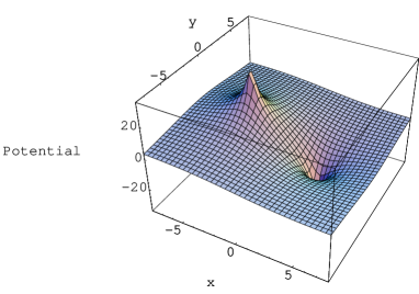
Figure 2: The potential (2.34).

continuum) particles, shown in fig. 2, has a form of the separated peak and the well. For sufficiently large $L$ the attraction by the well becomes strong enough for a discrete level to appear. Since a positive charge is attracted to the source at $x=L/2$ and is repulsed from the one at $x=-L/2$, its wave function $\psi_{+\,0}$ is localized near $x=L/2$. The wave function of the negative charge is localized near $x=-L/2$ and its energy is $\varepsilon_{-\,0}=-\varepsilon_{+\,0}$ by symmetry. The lowest positive- and negative-energy levels converge with the increase of $L$ and collide at zero for some critical

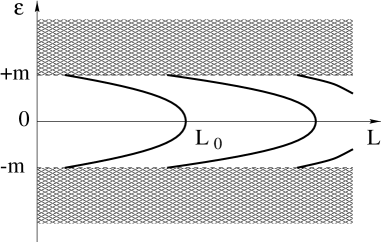
Figure 3: Spectrum of the Klein-Gordon equation for the potential (2.34).

value of $L=L_{0}$ (fig. 3). After that they do not disappear, but rather go off to the complex plane [9]. This behavior of the eigenvalues is generic for Klein-Gordon equation in strong electric fields [8, 9, 10]. For $L>L_{0}$ vacuum polarization can no longer be neglected and the external electric field creates a pair of charged particles in the vacuum. This effect is analogous to a pair creation in the field of a heavy ion with the nuclear charge $Z>137$ [9].

For large $L$ the ground state wave function is no longer localized near the well of the potential. Rather, the wave function has the shape with two bumps, like the one used in the qualitative arguments in the introduction. As $L$ grows, the charge leaks from the well to the region where the potential is peaked. This, at first sight, anti-intuitive behavior reflects a generic property of a charged Klein-Gordon particle to form a bound state in a sufficiently strong repulsive electric potential [9, 8, 10]. The fact that the charge is redistributed between the well and the peak of the potential can be proved by the following arguments. For $L=L_{0}$ both eigenvalues $\varepsilon_{-\,0}$ and $\varepsilon_{+\,0}$ are equal to zero and the Klein-Gordon equation formally has the form of the Schrödinger one:

$$\left[-\partial^{2}-\left(\frac{e^{2}q}{2\pi}\,\ln\frac{|x+L/2|}{|x-L/2|}\right)^{2}+m^{2}\right]\psi_{\pm\,0}=0~{}~{}~{}~{}(L=L_{0}).$$ (3.2)

The potential here has the shape of a symmetric double well. The ground state wave function is symmetrically distributed between the two wells. By continuity reasons, as $L$ is decreased, the charge begin to leak from the region near the repulsive source to the attractive one, and eventually all the positive charge is concentrated near $+L/2$ and the negative one near $-L/2$.

4 Screening of the logarithmic potential

So far, the vacuum sector was considered. However, when $e^{2}\ln(L\mu)\sim m$, the two-particle state

$$|2\rangle=a_{+\,0}^{\dagger}a_{-\,0}^{\dagger}|0\rangle$$ (4.1)

can become energetically more favorable, if the dynamical charges screen the sources and reduce the Coulomb energy by an amount sufficient to create a pair. The energy of the state (4.1) is

$$E_{\rm matter}=\varepsilon_{+\,0}-\varepsilon_{-\,0}$$ (4.2)

and the induced charge density is

$$\langle 2|J_{0}|2\rangle=2e\bar{\psi}_{+\,0}(\varepsilon_{+\,0}+e\varphi)\psi_{+\,0}+2e\bar{\psi}_{-\,0}(\varepsilon_{-\,0}+e\varphi)\psi_{-\,0}.$$ (4.3)

Vacuum contributions are neglected here.

The charged particles which cause the screening of the static charges are non-relativistic, since the screened electric fields are small everywhere, unlike the unscreened ones. Therefore, it is possible to use the non-relativistic approximation (3.1) to the Klein-Gordon equation. In this approximation, the wave functions $\psi_{\pm\,}$ – we omit the subscript $0$ for brevity – are normalized to $1/(2m)$, as follows from equation (2.23). For the sake of clarity it is, however, convenient to introduce new wave functions, $\psi_{\pm}^{\prime}=\sqrt{2m}\psi_{\pm}$, normalized to unity, as it is custom in the non-relativistic limit:

$$\int d^{2}x\,|\psi_{\pm}^{\prime}|^{2}=1,$$ (4.4)

whereas the induced charged density is

$$\left\langle J_{0}\right\rangle=e\left(|\psi_{+}^{\prime}|^{2}-|\psi_{-}^{\prime}|^{2}\right).$$ (4.5)

The total energy of the two-particle state is

$$E=2m+\frac{1}{2m}\!\int\!\!d^{2}x\,\Bigl{(}|\partial\psi_{+}^{\prime}|^{2}+|\partial\psi_{-}^{\prime}|^{2}\Bigr{)}-\!\frac{1}{4\pi}\!\int\!\!d^{2}xd^{2}y\left[\rho(x)+\left\langle J_{0}(x)\right\rangle\right]\ln|x-y|\left[\rho(y)+\left\langle J_{0}(y)\right\rangle\right].$$ (4.6)

This expression is obtained after $2m+\lambda_{+}+\lambda_{-}$ is substituted for $E_{{\rm matter}}$ in eq. (2.30), and the solution of the Poisson equation (2.31) is substituted for $\varphi$.

The energy (4.6) can be regarded as a functional of $\psi_{\pm}^{\prime}$. It is straightforward to check that the minimum of this functional is determined exactly by the Schrödinger equation (3.1). The coupled set of equations (2.31), (3.1), (4.4) and (4.5) constitute a rather complicated eigenvalue problem. The ground state corresponds to the global minimum, and can be found numerically. Instead of solving these equations directly we will suggest simple variational wave functions $\psi_{\pm}^{\prime}$ corresponding to a two-particle state whose energy does not grow with the separation of the external charges $L$.

We take the variational wave functions in a form of a superposition of states with charges $\pm e$ localized in the vicinity of the sources with charges $\pm eq,\;\;q<1$, see fig. 1. For symmetry reasons we take $\psi_{-}^{\prime}(x)=\psi_{+}^{\prime}(-x)$:

$$\psi_{+}^{\prime}(x)=\phi_{1}\left(x-\frac{L}{2}\right)+\phi_{2}\left(x+\frac{L}{2}\right),$$

$$\psi_{-}^{\prime}(x)=\phi_{2}\left(x-\frac{L}{2}\right)+\phi_{1}\left(x+\frac{L}{2}\right).$$ (4.7)

The functions $\phi_{1,2}$ are supposed to be well-localized and normalized to

$$\int d^{2}x\,\phi_{1,2}^{2}=\frac{1\mp q}{2}.$$ (4.8)

For large $L$ the overlap between $\phi_{1}$ and $\phi_{2}$ is exponentially small and can be neglected, therefore the wave functions (4.7) are normalized to unity. This ansatz corresponds to the distribution of charges described in the introduction. The $(1+q)/2$ portion of the dynamical charge is localized near the source of the opposite sign and the $(1-q)/2$ portion is localized near the one with the same sign.

Neglecting the exponentially small overlap of $\phi_{1,2}$ we get for the total charge density:

$$\rho(x)+\left\langle J_{0}(x)\right\rangle=e^{2}\left\{\left[q\,\delta\left(x+\frac{L}{2}\right)+\phi_{1}^{2}\left(x+\frac{L}{2}\right)-\phi_{2}^{2}\left(x+\frac{L}{2}\right)\right]\right.$$

$$\left.-\left[q\,\delta\left(x-\frac{L}{2}\right)+\phi_{1}^{2}\left(x-\frac{L}{2}\right)-\phi_{2}^{2}\left(x-\frac{L}{2}\right)\right]\right\}.$$ (4.9)

We see that the total charge density noticeably differs from zero only in the vicinity of the points $x=-L/2$ and $x=+L/2$. The screening of the delta-peaked external sources is achieved if the integral of the total charge density over the region much smaller than $L$ is zero. This is guaranteed by our choice of the normalization condition (4.8).

To make an estimate of the minimal energy of the two-particle screening state and, hence, of the critical separation between the external charges where the rising potential breaks up, we take a simple Gaussian ansatz for the wave functions $\phi_{1,2}$:

$$\phi_{1,2}(x)=\sqrt{\frac{1\mp q}{4\pi a_{1,2}^{2}}}\exp\left(-\frac{x^{2}}{4a_{1,2}^{2}}\right),$$ (4.10)

where the widths of the wave functions $a_{1,2}$ are the variational parameters. To make all integrals finite we shall temporarily introduce a Gaussian smearing of the external sources replacing

$$q\delta(x)\rightarrow\frac{q}{2\pi\zeta^{2}}\exp\left(-\frac{x^{2}}{2\zeta^{2}}\right),\;\;\;\;\zeta\rightarrow 0.$$ (4.11)

Now one has to substitute the trial wave functions (4.10) into the energy functional (4.6) and to find the best widths $a_{1,2}$ from its minimum. The integrals are readily performed by using the Fourier transforms. Recalling that the Fourier transform of $\ln(x^{2})/4\pi$ is $-1/k^{2}$ we get for the interaction or the potential energy term in the total energy (the last term in eq.(4.6)):

$$E_{pot}(L)=-e^{2}\int\frac{d^{2}k}{(2\pi)^{2}}\frac{e^{ik\cdot L}-1}{k^{2}}\left[q\,e^{-\frac{\zeta^{2}k^{2}}{2}}+\frac{1-q}{2}e^{-\frac{a_{1}^{2}k^{2}}{2}}-\frac{1+q}{2}e^{-\frac{a_{2}^{2}k^{2}}{2}}\right]^{2}.$$ (4.12)

The term proportional to $\exp(ik\cdot L)$ accounts for the interaction between the regions near $x+L/2$ and near $x-L/2$, while the subtracted term proportional to unity takes into account the self-interaction of charge distributions inside these regions.

Eq.(4.12) should be compared to the interaction of two bare external charges:

$$E_{bare}(L)=-e^{2}\int\frac{d^{2}k}{(2\pi)^{2}}\frac{e^{ik\cdot L}-1}{k^{2}}\left[q\,e^{-\frac{\zeta^{2}k^{2}}{2}}\right]^{2}=\frac{e^{2}q^{2}}{4\pi}\left(\ln\frac{L^{2}}{4\zeta^{2}}+\gamma_{E}\right).$$ (4.13)

Terms exponentially small in $L/\zeta$ have been neglected here. The integral (4.12) is immediately calculated using (4.13), yielding

$$E_{pot}=\frac{e^{2}}{4\pi}\left[q^{2}\ln\frac{L^{2}}{4\zeta^{2}}+\left(\frac{1-q}{2}\right)^{2}\ln\frac{L^{2}}{4a_{1}^{2}}+\left(\frac{1+q}{2}\right)^{2}\ln\frac{L^{2}}{4a_{2}^{2}}\right.$$

$$\left.+2q\frac{1-q}{2}\ln\frac{L^{2}}{2(\zeta^{2}+a_{1}^{2})}-2q\frac{1+q}{2}\ln\frac{L^{2}}{2(\zeta^{2}+a_{2}^{2})}-2\frac{1-q}{2}\frac{1+q}{2}\ln\frac{L^{2}}{2(a_{1}^{2}+a_{2}^{2})}\right].$$ (4.14)

The coefficient in front of $\ln L^{2}$ is zero, so that the energy is now independent of $L$, up to exponentially small corrections which are neglected. It is exactly the screening effect we are after, and it is due to the choice of the normalization of charge distributions, eq.(4.8). Neglecting also the spread of the external charges $\zeta^{2}$ as compared to $a_{1,2}^{2}$ we get

$$E_{pot}=\frac{e^{2}}{4\pi}\frac{1}{4}\left[2(1-q)(1+q)\ln(a_{1}^{2}+a_{2}^{2})-(1-q)(1+3q)\ln a_{1}^{2}-(1+q)(1-3q)\ln a_{2}^{2}\right.$$

$$\left.-2(1+3q^{2})\ln 2-4q^{2}\ln\zeta^{2}\right].$$ (4.15)

The kinetic energy term (the second term in eq.(4.6)) is

$$E_{kin}=\frac{1}{4m}\left(\frac{1-q}{a_{1}^{2}}+\frac{1+q}{a_{2}^{2}}\right)$$ (4.16)

The sum, $E_{kin}+E_{pot}$, has a minimum at

$$a_{1,2}^{2}=\frac{4\pi}{me^{2}}\frac{1\pm q+4q^{2}+(1\pm q)\sqrt{1+8q^{2}}}{4q^{2}(1\mp q)},$$ (4.17)

which should be substituted into (4.16) and (4.15) to get a variational estimate of the energy of the two-particle state screening the external charges. Naturally, the energy-at-rest, $2m$, should be added, too.

It follows from (4.17) that the distribution of the dynamical charge having the same sign as the external charge ($a_{1}$) is broader than that having the opposite charge ($a_{2}$). For example, if the external charge is one half of the dynamical charge ($q=1/2$) the same-charge cloud is about 2.5 times broader than the opposite-charge cloud. See the table, where examples for other values of $q$ are given.

Finally, the energy of the two-particle ground state can be written as

$$E=2m+\frac{e^{2}q^{2}}{4\pi}\left(\ln\frac{4\pi C_{q}^{2}}{me^{2}q^{2}4\zeta^{2}}+\gamma_{E}\right),$$ (4.18)

where $C_{q}$ is a number of the order of unity coming from substituting the best values of $a_{1,2}$ given by eq.(4.17) into $E_{kin}+E_{pot}$. Notice that the dependence on the spread of the delta-peaked external charges, $\zeta$, is the same as in the case of the bare charges, eq.(4.13). This is because the extended dynamical charge distribution cannot screen the logarithmic potential at small separations.

Table

$q$	$a_{1}\sqrt{\frac{me^{2}}{4\pi}}$	$a_{2}\sqrt{\frac{me^{2}}{4\pi}}$	$C_{q}$
0.1	7.96	6.53	0.536
$\frac{1}{3}$	3.49	1.85	0.589
$\frac{1}{2}$	3.19	1.26	0.649
$\frac{2}{3}$	3.44	0.976	0.717
0.9	5.65	0.776	0.824

The logarithmically rising potential between external charges at large separations breaks up when the bare energy (4.13) exceeds the energy of the screening state, eq.(4.18). It happens at the critical separation between the external charges

$$L_{c}=C_{q}\sqrt{\frac{4\pi}{me^{2}q^{2}}}\exp\left(\frac{4\pi m}{e^{2}q^{2}}\right).$$ (4.19)

Since we assume the non-relativistic limit, $m\gg e^{2}/4\pi$, this distance is exponentially large. Notice that the widths of the screening distributions $a_{1,2}$ as given by eq.(4.17) are much less than the critical distance $L_{c}$, which justifies neglecting of the overlaps between the screening clouds belonging to the two centers.

The numerical values of the coefficient $C_{q}$ are given in the table for certain values of $q$, together with the values of the widths $a_{1,2}$ measured in natural units of $\sqrt{me^{2}/4\pi}$. Since we have used a variational estimate for the ground state energy, the true minimum can be only lower, that is to say that the numerical coefficient $C_{q}$ of the order of unity in eqs.(4.18),(4.19) can be somewhat smaller than given in the table. However, the dependence on the algebraic parameters in these equations follow from the dimension analysis, and is of a general nature.

At $L\approx L_{c}$ the logarithmic growth of the potential stops; more precisely it slowly grows approaching its asymptotic value at infinity (4.18), the deviation corresponding to the residual forces between neutral charge clouds at $x=\pm L$.

5 Path-integral approach

The arguments we used above are in essence the variational ones. For this reason, we preferred to use the Hamiltonian formalism. Although the discussion of the screening from the path-integral point of view is beyond the scope of the present paper, we would like to outline how the main ingredients of our analysis can be derived from the path integral. Here we consider only the vacuum sector.

The vacuum average of the Wilson loop infinitely stretched in the time direction, which determines the energy of two static charges, is given by the path integral

$$Z = \int DAD\Phi^{\dagger}D\Phi\,\exp\left\{i\int d^{4}x\,\left[-\frac{1}{4}\,F_{\mu\nu}F^{\mu\nu}+(D_{\mu}\Phi)^{\dagger}D^{\mu}\Phi-m^{2}\Phi^{\dagger}\Phi\right]\right.$$ (5.1)

$$\left.+iqe\int dx^{0}\,\Bigl{(}A_{0}(x^{0},-L/2)-A_{0}(x^{0},+L/2)\Bigr{)}\right\}.$$

Integration over the scalar fields induces an effective action for the gauge potentials:

$$\Delta S=i\>{\rm Tr}\,\ln(-D^{2}-m^{2}+i0).$$ (5.2)

The next step, justified by the smallness of the coupling, is to calculate the remaining integral over $A_{\mu}$ in the saddle-point approximation. This amounts to solving classical equations of motion taking into account the induced action (5.2) and the source term in (5.1). We are going to show that these saddle-point equations are nothing but the ones derived in Secs. 2, 3 in the Hamiltonian formalism.

Owing to the symmetries of the problem the classical fields are time-independent, and $A_{i}^{\rm cl}=0$. For $A_{0}^{\rm cl}$ we get the Poisson equation,

$$-\partial_{i}\partial_{i}A_{0}^{\rm cl}+\rho+\left\langle J_{0}\right\rangle=0,$$ (5.3)

where $\rho$ is the same as in (2.8) and the induced charge density is

$$\left\langle J_{0}\right\rangle=i\,\frac{\delta}{\delta A_{0}^{\rm cl}}\,\>{\rm Tr}\,\ln(-D^{2}-m^{2}+i0)=e\left.\Bigl{(}\overrightarrow{D}_{0}G(x,y)+G(x,y)\overleftarrow{D}_{0}\Bigr{)}\right|_{x=y},$$ (5.4)

where

$$G(x,y)=\left\langle x\left|\frac{1}{-D^{2}-m^{2}+i0}\right|y\right\rangle.$$ (5.5)

We leave the calculation of the induced charge density to Appendix, where we show that it reduces to solving the Klein-Gordon equation (2.21) with $\varphi$ replaced by $A_{0}^{\rm cl}$ and that the saddle-point equation (5.3) coincides with (2.31).

6 Conclusions

To summarize, the infinitely rising potential between fractionally charged external (probe) sources is screened in (2+1)-dimensional scalar QED. Of course, if the mass of the dynamical fields is large, the rising potential persists at intermediate scales. The critical distance is exponentially large in $m/e^{2}$, in contrast to 3D spinor QED where the screening length is of the order of $1/e^{2}$ [6].

The screening is a typical quantum-mechanical effect: the wave functions of the screening particles are superpositions of two distinctive bumps localized near external sources of both signs and carrying fractional charge. In case of a half-integer charge of the probe ($q=\frac{1}{2}$) the bumps carry charges $\frac{3}{4}$ and $\frac{1}{4}$, so that the total probability is unity but the external sources are completely screened, see fig. 1.

It is interesting that the screening effect would be probably not easy to observe from Euclidean lattice simulations of the theory (given by the partition function (5.1)). Indeed, the essence of the mechanism is a formation of two bumps in the screening wave functions, which is a kind of tunneling effect. The larger the separation between sources $L$, the longer computer time one would need for this effect to come into action, with the time growing exponentially with $L$.

Nevertheless, it would be very useful to check the screening of fractional charges by lattice simulations, in view of apparent analogies with a more difficult case of non-Abelian gauge theories.

Acknowledgments

D.D. would like to thank Victor Petrov for many discussions in the past that stimulated this investigation. K.Z. is grateful to NORDITA for hospitality while this work was in progress. The work of K.Z. was supported in part by NATO Science Fellowship, CRDF grant 96-RP1-253, INTAS grant 96-0524, RFFI grant 97-02-17927 and grant 96-15-96455 for the promotion of scientific schools.

Appendix A Eigenfunction expansion of induced charge density

Since the background field is time-independent, the eigenmodes of the operator $-D^{2}-m^{2}$,

$$(-D^{2}-m^{2})\tilde{u}=\kappa\tilde{u},$$ (A.1)

have the form

$$\tilde{u}={\,\rm e}\,^{i\varepsilon x^{0}}u,$$ (A.2)

where $u$ depends only on spatial coordinates and satisfies the equation

$$\left[(\varepsilon+eA_{0}^{\rm cl})^{2}+\partial_{i}\partial_{i}-m^{2}\right]u_{n}=\kappa_{n}u_{n}.$$ (A.3)

The eigenvalues $\kappa_{n}$ are the functions of $\varepsilon$. The eigenfunctions $u_{n}$ are supposed to be normalized to unity for any given $\varepsilon$.

The Green function (5.5) can be expanded in the eigenfunctions as

$$G(x,y)=\int_{-\infty}^{+\infty}\frac{d\varepsilon}{2\pi}\,{\,\rm e}\,^{i\varepsilon(x^{0}-y^{0})}\sum_{n}\frac{u_{n}(x)\bar{u}_{n}(y)}{\kappa_{n}(\varepsilon)+i0}.$$ (A.4)

The integral over $\varepsilon$ can be calculated closing the contour of integration in the upper or in the lower complex half-plane, depending on the sign of $x^{0}-y^{0}$. The charge density is defined in the limit $x^{0}\rightarrow y^{0}$ and, in principle, depends on how this limit is approached. The correct prescription is to take the limit symmetrically in $x^{0}-y^{0}$.

The integrand in (A.4) has a pole if $\kappa_{n}(\varepsilon)=0$. The values of $\varepsilon$ which satisfy this condition are determined exactly by equation (2.21). The only difference is in the normalization of the functions $u_{n}$ and $\psi_{n}$:

$$\psi_{n}=\frac{u_{n}}{\sqrt{|N_{n}|}},$$ (A.5)

$$N_{n}=2\int d^{3}x\,\bar{u}_{n}(\varepsilon_{n}+eA_{0}^{\rm cl})u_{n}.$$ (A.6)

For sufficiently weak fields all poles lie on the real axis. Near a given pole one has

$$\kappa_{n}(\varepsilon)=N_{n}(\varepsilon-\varepsilon_{n})+\ldots,$$ (A.7)

since, as it follows from eq. (A.3),

$$\frac{d\kappa_{n}}{d\varepsilon}=N_{n}.$$

For weak fields $N_{n}$ is positive for positive $\varepsilon$ and negative for negative ones. Therefore, the contour of integration in eq. (A.4) passes the poles on the positive semiaxis from above and the ones

Figure 4: The contour of integration in the complex $\varepsilon$ plane.

on the negative semiaxis from below (fig. 4). By continuity, this rule remains valid for strong fields until the positive and the negative poles collide. It can be shown that exactly when two poles collide (fig. 3) and go off to the complex plane the integral $N_{n}$ turns to zero [9].

As a consequence of eqs. (A.7), (A.5), the functions $u_{n}$ are replaced by $\psi_{n}$ in the residues of the integral (A.4). Taking into account that the covariant derivative $D_{0}$ acts on the eigenfunctions (A.2) of the Klein-Gordon operator as $i(\varepsilon+eA_{0}^{\rm cl})$, we find for the induced charge density:

$$\left\langle J_{0}\right\rangle=e\sum_{n}\bar{\psi}_{n}(\varepsilon_{n}+eA_{0}^{\rm cl})\psi_{n}.$$ (A.8)

It can be checked that this expression coincides with the vacuum average of the charge density operator defined in sec. 2.

The above consideration implies that all eigenvalues of the Klein-Gordon equation lie on the real axis, which is true for sufficiently weak fields, that is, for sufficiently small separation between external charges $L$. For very strong fields (at $L>L_{0}$) some poles move to the complex plane, as discussed in Sec. 3, which invalidates the analysis above. This signals that for large $L$ the ground state is rearranged and the true vacuum is different from an empty state with no dynamical charges.

References

- [1] S. Coleman, R. Jackiw and L. Susskind, Ann. Phys. 93 (1971) 267.
- [2] D.J. Gross, I.R. Klebanov, A.V. Matytsin and A.V. Smilga, Nucl. Phys. B461 (1996) 109, hep-th/9511104.
-
[3]
R. Rodriguez and Y. Hosotani, Phys. Lett. B375 (1996) 273,
hep-th/9602029;
C. Adam, Phys. Lett. B394 (1997) 161, hep-th/9609155. -
[4]
Y. Frishman and J. Sonnenschein, Nucl. Phys. B496 (1997) 285,
hep-th/9701140;
S. Dalley, Phys. Lett. B418 (1998) 160, hep-th/9708115;
A. Armoni, Y Frishman and J. Sonnenschein, Phys. Rev. Lett. 80 (1998) 430, hep-th/9709097; hep-th/9807022. - [5] D. Kutasov and A. Schwimmer, Nucl. Phys. B442 (1995) 447, hep-th/9501024.
-
[6]
E. Abdalla and R. Banerjee, Phys. Rev. Lett. 80 (1998) 238,
hep-th/9704176;
E. Abdalla, R. Banerjee and C. Molina, hep-th/9808003. -
[7]
I. Affleck, J.A. Harvey and E. Witten, Nucl. Phys. B206 (1982) 413;
A.J. Niemi and G.W. Semenoff, Phys. Rev. lett. 51 (1983) 2077;
A.N. Redlich, Phys. Rev. D29 (1984) 2366. - [8] A.B. Migdal, Sov. Phys. JETP 34 (1972) 1184 [Zh. Eksp. Teor. Fiz. 61 (1972) 2209].
- [9] Ya.B. Zel’dovich and V.S. Popov, Sov. Phys. Uspekhi 14 (1972) 673 [Usp. Fiz. Nauk 105 (1971) 403].
- [10] W. Greiner, B. Müller and J. Rafelski, Quantum Electrodynamics of Strong Fields (Springer-Verlag, 1985).