$1/f$ Noise in Fractal Quaternionic Structures

Abstract

We consider the logistic map over quaternions $\mathbb{H}\sim\mathbb{R}^{4}$ and different 2D projections of Mandelbrot set in 4D quaternionic space. The approximations (for finite number of iterations) of these 2D projections are fractal circles. We show that a point process defined by radiuses $R_{j}$ of those fractal circles exhibits pure $1/f$ noise.

Keywords: $1/f$ noise, point process, logistic map, Mandelbrot set, quaternions, hypercomplex numbers

PACS: 05.40.–a, 05.45.Df, 02.50.Ey

1 Introduction

$1/f$ noise is observed in large diversity of real life and artificial systems, which behavior is usually defined by a complex interaction of many components. Complexity of the system usually assumes that long-term correlations are observed. Examples are processes and experimental data in condensed matter, traffic flow, quasar emissions, music, biological and medical systems, economic and financial data, human cognition and even distribution of prime numbers (see [1] and references herein).

Fluctuations of signals defined by time series obtained from such systems are found to be characterized by a power spectral density $S(f)$ diverging at low frequencies $f$ like $1/f^{\alpha}$, here $\alpha$ is some real parameter. $1/f$ ($\alpha\approx 1$) noise is an intermediate between the white noise ($\alpha=0$) with no correlation in time and the random walk (Brownian motion) noise ($\alpha=2$) with no correlation between increments. Note that Brownian motion can be obtained integrating white noise and that taking the integral of the signal increases the exponent $\alpha$ by 2 while the inverse operation of differentiation decreases it by 2.

Parameter $\alpha$ is closely related to the Hurst exponent $H$. It is known that fluctuations which are fractionally homogeneous, i.e. unifractal or uniscaling, can be quantified by a single coefficient $H$ and a single exponent $\alpha$ [2].

Possible generalization leads to multiscaling or multifractals, with the exponent H dependant on time. Therefore multifractal processes are characterized by a set of scaling relations or power laws with correspondingly many exponents $\alpha$ [3].

2 Point processes and $1/f$ noise

In many cases, the intensity of some current can be represented by a sequence of random (however, as a rule, mutually correlated) or pseudo-periodic pulses $A_{k}(t-t_{k})$. Here the function $A_{k}(\varphi)$ represents the shape of the $k$-th pulse having an influence to the current $I(t)$ in the region of transit time $t_{k}$. The intensity of the current in some space cross-section may, therefore, be expressed as

$$I(t)=\sum_{k}A_{k}(t-t_{k}).$$

It is easy to show that the shapes of the pulses mainly influence the high frequency, $f\geq\Delta t_{p}$ with $\Delta t_{p}$ being the characteristic pulse length, power spectral density of $I(t)$ while fluctuations of the pulse amplitudes result, as a rule, in the white or Lorentzian but not $1/f$ noise.

Therefore, we restrict our analysis to the fluctuations due to the correlations between the transit times $t_{k}$ and hence we can replace the function $A_{k}(t-t_{k})$ by the Dirac delta function $\delta(t-t_{k})$. The current (see Fig. 1) is then expressed as

$$I(t)=\sum_{k}\delta(t-t_{k}).$$ (1)

Following this approach, instead of current $I(t)$, we further deal with point process, defined by the sequence $t_{1},t_{2},\ldots,t_{N},\ldots$.

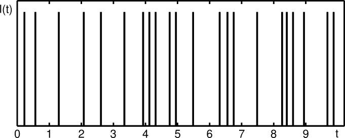
Figure 1: Current $I(t)$ vs time $t$ defined by (1) formula. Such dependencies appear when registering the consecutives heart beats, cars on a highway passing through the reference point, transactions in financial markets etc.

The power spectral density of the current (1) is defined as

$$S(f)=\lim_{N\to\infty}\frac{2}{t_{N}}\left|\sum_{k=1}^{N}e^{\displaystyle-i2\pi ft_{k}}\right|^{2}$$ (2)

where $[t_{1},t_{N}]$ is assumed to be the interval of observation.

In this approach the power spectral density of the signal depends on the statistics and correlations of point process (the transit times $t_{k}$) only. It is well known that sequence of random, Poisson, transit times generates white (shot) noise, for example.

In [4] we proposed simple analytically solvable model for producing point process resulting in $S(f)\sim 1/f$ ($\alpha=1$) noise. Discussion on the origin and universality of $1/f$ noise was continued in [5, 6]. Some further work, related to the applications of the theory of point processes and $1/f$ noise to econophysics, was done in [7, 8].

3 Quaternions and other hypercomplex numbers

Complex numbers $\mathbb{C}\sim\mathbb{R}^{2}$, along to their real predecessors $\mathbb{R}$, are widely used in nowadays mathematical modeling and scientific computing. Beside others, they have important applications in theories of complex systems, fractals and signal processing: famous Mandelbrot and Julia fractal sets are defined in $\mathbb{C}$, spectrum (Fourier transform) is defined as integral of complex function etc.

There are some clues that we should not stop with the computations in $\mathbb{R}$ and $\mathbb{C}$, and that further generalization to quaternions $\mathbb{H}\sim\mathbb{R}^{4}$ (introduced by Hamilton) or even octonions $\mathbb{G}\sim\mathbb{R}^{8}$ (introduced by Graves) are particulary interesting and valuable, even though the role of these hypercomplex numbers is not widely understood yet.

In order to define hypercomplex algebras, one has to consider not only two algebraic operations $+$ and $\times$, but also one geometric map: $x\mapsto\bar{x}$, where $\bar{x}$ denotes the conjugate vector of $x$.

The three operations are defined recursively as we define the algebras, in the following manner. Let $A_{k}$ be the real hypercomplex algebra of dimension $2^{k}$, $k\geq 1$. It is constructed recursively as $A_{k}=A_{k-1}\times A_{k-1}$ by means of the three following operations:

addition:multiplication: (a,b)+(c,d) = (a+c,b+d),

conjugacy:multiplication:$$\overline{(a,b)}$$(a,b)+(c,d) = (¯a,-b),

$$\mbox{multiplication:}\quad(a,b)\times(c,d) = (ac-\bar{d}b,da+b\bar{c}),$$

where $ac$ denotes $a\times c$ in $A_{k-1}$. For $k=0$, $A_{0}$ is taken to be the field $\mathbb{R}$ with the arithmetic operations $+$ and $\times$, the conjugacy map being the identity on $\mathbb{R}$: $a\mapsto\bar{a}=a\in\mathbb{R}$. This construction is known to algebraists as the Cayley-Dickson doubling process.

About computations with hypercomplex numbers, and why only real numbers, complex numbers, quaternions and octions are suitable for computations see [9, 10] and references herein.

Explicitly multiplication in $\mathbb{H}$ can be expressed as $(a,b,c,d)\times(a^{\prime},b^{\prime},c^{\prime},d^{\prime})=(a^{\prime\prime},b^{\prime\prime},c^{\prime\prime},d^{\prime\prime})$, with

$$a^{\prime\prime}=aa^{\prime}-bb^{\prime}-cc^{\prime}-dd^{\prime}$$

$$b^{\prime\prime}=ab^{\prime}+ba^{\prime}+cd^{\prime}-dc^{\prime}$$

$$c^{\prime\prime}=ac^{\prime}+ca^{\prime}+db^{\prime}-bd^{\prime}$$

$$d^{\prime\prime}=ad^{\prime}+da^{\prime}+bc^{\prime}-cb^{\prime}$$

4 $1/f$ noise in quaternionic Mandelbrot set

We consider the logistic map over quaternions $\mathbb{H}\sim\mathbb{R}^{4}$

$$z_{k+1}=rz_{k}(1-z_{k}),\quad r,z_{k}\in\mathbb{H},\quad k=0,1,\ldots.$$ (3)

with given initial value $z_{0}$, for example $z_{0}=(0.5,0,0,0)$. The logistic map (3) has been extensively studied over $\mathbb{R}$ (real numbers) and $\mathbb{C}$ (complex numbers). Despite its great simplicity this map exhibits an extremely complex behaviour. The study of (3) on $\mathbb{R}$ gives birth to the Feigenbaum tree while the analysis of (3) on $\mathbb{C}$ leads to the famous Mandelbrot and Julia fractal sets.

Further we deal with 2D projections of Mandelbrot set in 4D quaternionic space. Any two components of $r$ are set to zero, while the remaining two vary. For example,

$${\cal{M}}_{12}=\left\{(r_{1},r_{2}):r=(r_{1},r_{2},0,0),\lim_{k\to\infty}|z_{k}|<\infty\right\},$$

$${\cal{M}}_{24}=\left\{(r_{2},r_{4}):r=(0,r_{2},0,r_{4}),\lim_{k\to\infty}|z_{k}|<\infty\right\}.$$

Note that ${\cal{M}}_{12}$ is just the famous Mandelbrot set in $\mathbb{C}$. We also show that ${\cal{M}}_{12}={\cal{M}}_{13}={\cal{M}}_{14}$ and ${\cal{M}}_{23}={\cal{M}}_{24}={\cal{M}}_{34}$.

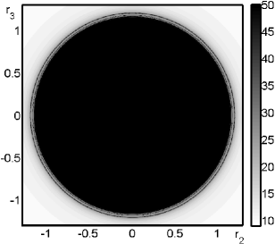
Figure 2: Approximation (after $50$ iterations) of Mandelbrot set ${\cal{M}}_{23}$ (one gets exactly the same for ${\cal{M}}_{24}$ or ${\cal{M}}_{34}$).

The approximations (for finite number of iterations) of Mandelbrot set ${\cal{M}}_{23}={\cal{M}}_{24}={\cal{M}}_{34}$ (near its boundary) are fractal circles (see Fig. 2), dependant only on radius $R=\sqrt{r_{2}^{2}+r_{3}^{2}}$.

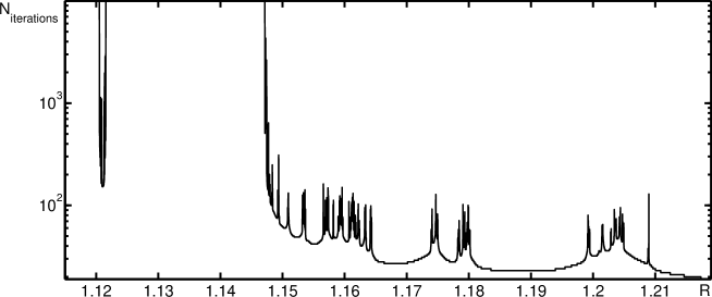
Figure 3: The number of iterations needed to reach $|z_{k}|>10^{10}$ plotted vs radius $R$ when computing ${\cal{M}}_{23}$.

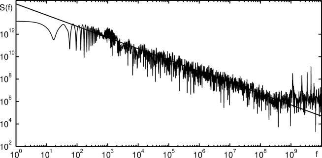
Figure 4: Power spectral density $S(f)$, defined by (4), vs frequency $f$ with $N=796474$. The plot is compared to the function $1/f$.

Define the point process $R_{j}$ as the values of radius of each circle – mathematically they are the values of $R$, small change of which result in significant change of number of iterations needed for $|z_{k}|$ to reach “infinity” ($10^{10}$ for example). The values $R_{j}$ correspond to peaks in Fig. 3.

According to (2), the power spectral density of such point process is defined as

$$S(f)\approx\frac{2}{R_{N}-R_{1}}\left|\,\sum_{j=1}^{N}e^{\displaystyle-i2\pi fR_{j}}\,\right|^{2},$$ (4)

here $N$ is the volume of point process data ($N\to\infty$ as $R_{j}$ recording resolution increases).

We obtain (see Fig. 4) that $S(f)\sim 1/f$, i. e. radiuses $R_{j}$ of fractal circles in Mandelbrot set ${\cal{M}}_{23}$ exhibit pure $1/f$ noise ($\alpha=0$) or unifractal noise.

References

- [1] B. Pilgram, and D. T. Kaplan, Physica D, 114, 108–122 (1998).
- [2] C.-K. Peng, S. Havlin, H. E. Stanley, and A. L. Goldberger, Chaos, 5, 82–87 (1995).
- [3] B. B. Mandelbrot, Multifractals and Noise, Springer, New York, 1999.
- [4] B. Kaulakys, and T. Meškauskas, Phys. Rev. E 58, 7013–7019 (1998); adap-org/9812003; B. Kaulakys, Phys. Lett. A 257, 37–42 (1999); adap-org/9806004; adap-org/9907008.
- [5] B. Kaulakys, and T. Meškauskas, Microel. Reliab. 40, 1781–1785 (2000); cond-mat/0303603; B. Kaulakys, Microel. Reliab. 40, 1787–1790 (2000); cond-mat/0305067; B. Kaulakys and J. Ruseckas, Phys. Rev. E 70, 020101(R) (2004); cond-mat/0408507; B. Kaulakys, V. Gontis, M. Alaburda, Phys. Rev. E 71, 051105 (2005); cond-mat/0504025.
- [6] B. Kaulakys, and T. Meškauskas, “Models for generation of noise,” in Noise in Physical Systems and Fluctuations, edited by C. Surya, ICNF 1999 Conference Proceedings 15th International Conference on Noise in Physical Systems and Fluctuations, HongKong, China, 1999, pp. 375–378.
- [7] V. Gontis, and B. Kaulakys, Physica A 343, 505–514 (2004); cond-mat/0303089.
- [8] V. Gontis, and B. Kaulakys, Physica A 344, 128–133 (2004); cond-mat/0412723.
- [9] F. Chaitin-Chatelin, T. Meškauskas, and A. N. Zaoui, CERFACS Technical Report TR/PA/00/74, http://www.cerfacs.fr/algor/reports/2000, (2000).
- [10] F. Chaitin-Chatelin, and T. Meškauskas, Nonlinear Analysis, 47, 3391–3400 (2001).