Statistical properties of braid groups
in locally free approximation

A.M. Vershik ^1,∗, S. Nechaev ^2,3 and R. Bikbov ³

¹ St. Petersburg Branch of Steklov Mathematical Institute, Fontanka 27,
119011 St.Petersburg, Russia

² UMR 8626, CNRS-Université Paris XI, LPTMS, Bat.100, Université Paris Sud,
91405 Orsay Cedex, France

³ L.D. Landau Institute for Theoretical Physics, Kosygin str. 2,
117940 Moscow, Russia

Statistical and probabilistic characteristics of locally free group with growing number of generators are defined and their application to statistics of braid groups is given.

 

^∗ Also at: Institut des Hautes Études Scientifiques, 35, route de Chartres,
                 91440 Bures-sur-Yvette, France

1 Introduction

The theory of knots, since works of Artin, Alexander, Markov (jr.) and others, is traditionally connected to the braid group $B_{n}$ (see for review [Bi1]). Jones polynomials [Jo] and a whole subsequent progress in knot theory is based on representations of braid groups and Hecke algebras. But alongside with a known problem of construction of topological invariants of knots and links, it should be noted a number of similar, but much less investigated problems. We mean calculation of a probability of a knot formation in a given homotopic type with respect to a uniform measure on a set of all closed nonselfintersecting contours of a fixed length on a lattice. The given problem, known as a ”knot entropy” problem so far has not an adequate mathematical apparatus and since recently has been studied mainly by numerical methods [FK+]. Nevertheless it is clear that the mentioned set of problems is connected by large to random walks on noncommutative groups.

The last years have been marked by occurrence of a great number of problems of a physical origin, dealing with probabilistic processes on noncommutative groups. Let us mention some examples, important for us. First of all, that are the problems of statistics and topology of chain molecules and related statistical problems of knots (see, for example, [Ne]), as well as the classical problems of the random matrix theory and localization phenomena [LGP].

In a set of works [GN] a problem concerning calculation of a mathematical expectation of a ”complexity” of randomly generated knot had been formulated, where the degree of any known algebraic invariant (polynomials of Jones, Alexander, HOMFLY and other) had been served for the characteristics of complexity.

As to the theory of random walk on braid groups, a particular number of results devoted to the investigation conditional limiting behavior of Brownian bridges on the group $B_{3}$ is known only [NGV]. Thus, neither Poisson boundary, nor explicit expression of harmonic functions for braid groups are so far found.

In the present paper we consider statistical properties of locally free and braid groups following the idea of the first author (A.V.) developed in [VKai] and extended in the papers [Ve1, DN1, DN2]. For study of braid groups we introduce the concept of so named locally free groups, which is the particular case of local groups in sense of works [Ve1, Ve2]. This concept gives us very useful tool for bilateral approximations for the number of nonequivalent words in the braid groups and semi–groups. Very important and apparently rather new aspect of this problem consists in passing to the limit $n\to\infty$ in the group $B_{n}$; just this limit is considered in our work. We found rather unexpected stabilization of various statistical characteristics of the local groups in this limit.

In [Ve2] the systematical approach to computation of various numerical characteristics of countable groups is proposed. The essence of this approach deals with simultaneous consideration of three numerical constants, properly characterizing the logarithmic volume, as well as the entropy and the escape (the drift) of the uniform random walk on the group. It happens that the inequality which relates these three constants proved in [Ve1, Ve2] reflects the deep statistical properties of local groups. The evaluation of number of words, entropy and other statistical characteristics for the locally free groups permits one to estimate the appropriate characteristics for the braid groups. So, the locally free groups play the role of the approximant to the braid groups. At the same time the study of locally free groups has appeared to be useful for other models of statistical physics, connected with problems of directed growth, theory of parallel computations and etc. (see [Vi] for review).

2 Main definitions and statement of a problem

Definition 1 (Artin braid group)

The braid group $B_{n+1}$ of $n+1$ ”strings” has $n$ of generators $\{\sigma_{1},\ldots,\sigma_{n}\}$ with the following relations:

$$\left\{\begin{array}[]{ll}\sigma_{i}\sigma_{i+1}\sigma_{i}=\sigma_{i+1}\sigma_{i}\sigma_{i+1}&\qquad(1\leq i<n)\\ \sigma_{i}\sigma_{j}=\sigma_{j}\sigma_{i}&\qquad(|i-j|\geq 2)\\ \end{array}\right.$$ (1)

In connection with general definitions of the braid group, there exists an extensive literature—see [Bi1]; for the last work on the normal forms of words, we shall note [Bi2].

The element of the braid group $B_{n}$ is set by a word in the alphabet $\{\sigma_{1},\ldots,\sigma_{n};\break\sigma_{1}^{-1},\ldots,\sigma_{n}^{-1}\}$—see fig.1

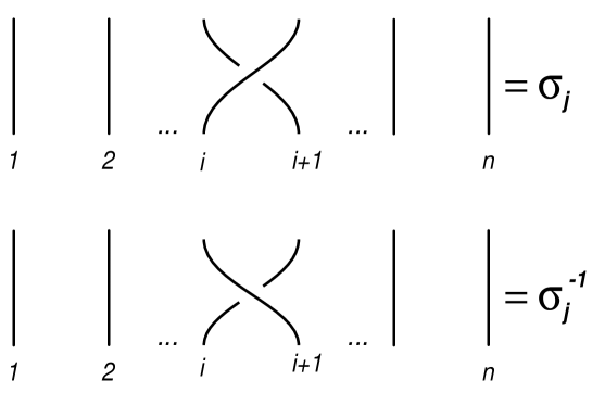
Figure 1: Graphic representation of generators of braid group $B_{n+1}$

By length $N$ of a record of a braid we call just a length of a word in a given record of the braid, and by irreducible length (or simple length) – the minimal length of a word, in which the given braid can be written. The irreducible length can be also viewed as a distance from the unity on the Cayley graph of the group. Graphically the braid it is represented by a set of strings, going from above downwards in accordance with growth of a braid length.

Closed braid is received by gluing the ”top” and ”bottom” free ends on a cylinder. Closed braid defines a link (in particular, a knot). Homotopic type of the link can be described in terms of algebraic characteristics of a braid [Jo].

Now we define a concept of a locally free group, which is a special case of noncommutative local group [Ve1, Ve2].

Definition 2 (Locally free group)

By a locally free group ${\cal LF}_{n+1}$ with $n$ generators $\{f_{1},\ldots,f_{n}\}$ we denote a group, determined by following relations:

$$f_{j}f_{k}=f_{k}f_{j}\qquad\mbox{for all}\qquad|j-k|\geq 2,\quad\{j,k\}=1,...n$$ (2)

Each pair of neighboring generators $(f_{j},f_{j\pm 1})$ produces a free subgroup of a group ${\cal LF}_{n}$. Similarly the locally free semi–group ${\cal LF}_{n}^{+}$ is defined.

The concept, equivalent to the concept of locally free semi–group ${\cal LF}_{n}^{+}$ has occurred earlier in work [CF], devoted to the investigation of combinatoric properties of substitutions of sequences and so named ”partially commutative monoids” (see [Vi] and references there). Especially productive becomes the geometrical interpretation of monoids in a form of a ”heap”, offered by G.X. Viennot and connected with various questions of statistics of directed growth and parallel computations. The case of a group (instead of semi–group) introduces a number of additional complifications to the model of a heap and apparently has not been considered in the literature. We touch it in more details below.

Obviously, the braid group $B_{n}$ is the factor–group of a locally free free group ${\cal LF}_{n}$, since it is received by introducing the Yang–Baxter (braid) relations. It has been realized also, that the group ${\cal LF}_{n}$ is simultaneously the subgroup of the braid group.

Lemma 1

Consider a subgroup $\overline{B}_{n}$ of the group $B_{n}$, over squares of generators $B_{n}:\;\overline{B}_{n}=\left<\overline{\sigma}_{1},...,\overline{\sigma}_{n-1}|\overline{\sigma}_{i}=\sigma_{i}^{2},\;i=1,...,n\right>$. The correspondence $\overline{\sigma}_{i}\leftrightarrow f_{i}$ sets the isomorphism of the groups $\overline{B}_{n}$ and ${\cal LF}_{n}$.

Proof. For the proof of this fact it is sufficient to check that between the generators $\overline{\sigma}_{i}=\sigma_{i}^{2}$ and $\overline{\sigma}_{i+1}=\sigma_{i+1}^{2}$ there are no any nontrivial relations. Thus, it is sufficient to restrict ourselves to consideration of a group $B_{3}$, or to be more precise, of its subgroup $\overline{B}_{3}$. Consider the Burau representation

$$\sigma_{1}(t)=\left(\begin{array}[]{cc}1&0\\ t&-t\end{array}\right);\qquad\sigma_{2}(t)=\left(\begin{array}[]{cc}-t&1\\ 0&1\end{array}\right),$$

being the exact representation of $B_{3}$ over $C[t]$. It is obvious that

$$\overline{\sigma}_{1}=\sigma_{1}^{2}(t)=\left(\begin{array}[]{cc}1&0\\ t-t^{2}&t^{2}\end{array}\right);\qquad\overline{\sigma}_{2}=\sigma_{2}^{2}(t)=\left(\begin{array}[]{cc}t^{2}&-t+1\\ 0&1\end{array}\right)$$ (3)

Putting $t=-1$, we see that (3) is reduced up to

$$f_{1}=\sigma_{1}^{2}(-1)=\left(\begin{array}[]{cc}1&0\\ -2&1\end{array}\right);\qquad f_{2}=\sigma_{2}^{2}(-1)=\left(\begin{array}[]{cc}1&2\\ 0&1\end{array}\right),$$

which are the generators of free group, $\Gamma_{2}$.  

It should be noted, that the matrices $\left(1\;2\atop 0\;1\right)$ and $\left(\;1\;\;0\atop-2\;1\right)$ are the generators of a free group. This fact was proved apparently for the first time by I. Sanov [Sa].

Corollary 1

Locally free group ${\cal LF}_{n}$ is simultaneously over– and subgroup of the braid group $B_{n}$.

This consequence will be hereafter used for transmitting the estimates from the locally free group to the braid group. The geometrical interpretation of the group ${\cal LF}_{n+1}$ is shown in fig.2.

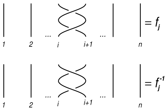
Figure 2: Graphic representation of generators of locally–free group ${\cal LF}_{n+1}$

Let us introduce also a concept of a locally free group of restricted order.

Definition 3

We call the group ${\cal LF}_{n}^{(r)}$ with generators $\{f_{1},\ldots,f_{n}\}$ and relations $(f_{i})^{r}=1\;(i=1,...,n)\;f_{i}f_{j}=f_{j}f_{i},\;|i-j|\geq 2$ a locally free group of restricted order $r$. The neighboring generators $f_{i},f_{i\pm 1}$ form the free product of ${{\sf Z\kern-3.20007ptZ}}/r{{\sf Z\kern-3.20007ptZ}}$.

In addition, another semi–group ${\cal LFP}_{n}^{+}$ emerges while imposing ”projective” relations $(f_{i})^{2}=f_{i}$.

Let us formulate the main problems concerning the determination of asymptotic characteristics of locally free and similar groups.

1. Asymptotics of number of words in a group. Let $G$ be the group with fixed framing $\{f_{1},...,f_{n}\}$. The definition following hereafter makes sense for any groups with fixed and finite set of generators. Denote by $K(g)$ and call the length $K(g)$ the minimal length of word $g$, written in terms of generators $\{g_{1},...,g_{n};g_{1}^{-1},...,g_{n}^{-1}\}$. The length defines the metrics (the metrics of words [Gr]) on the group.

Denote by $V(G,K)$ the number of elements of group $G$ of length $K$.

Definition 4

Call $v(G,K)$ the logarithmic volume of a group with respect to the given group $G$:

$$v(G)=\lim_{K\to\infty}\frac{\log V(G,K)}{K}$$ (4)

where the limit exists—see [Ve2]. We call $G$ as the group of exponential growth if $v>0$.

In Section 3 we investigate the asymptotic behavior of $v(B_{n})$, $v({\cal LF}_{n})$ at $K\to\infty$, in the limit $n={\rm const}\gg 1$.

2. Random walk and average drift on a group. Consider the (right–hand side) random walk on any group $G$ with fixed framing $\{g_{1},...,g_{n};g_{1}^{-1},...,g_{n}^{-1}\}$, i.e. regard the Markov chain with following transition probabilities: the word $w$ transforms into $w\,g^{\pm 1}$ with the probability $\frac{1}{2n};\;i=1,...,n$. Similarly one can build a left–hand Markov chain.

Let $L(G,N)$ be a mathematical expectation of a length of a random word, obtained after $N$ steps of random walk on the group $G$.

Definition 5

Call $l(G,N)$ the drift on the group $G$ (see [Ve2]):

$$l(G)=\limsup_{N\to\infty}\frac{L(G,N)}{N}$$ (5)

Thus, the drift is the average speed of a flow to the infinity in the metrics of words.

In Section 4 we calculate the drift $l({\cal LF}_{n})$ on the locally free group and its limit for $n={\rm const}\gg 1$.

3. Entropy of a random walk on a group. Let $\mu^{N}$ be the $N$–time convolution of a uniform measure $\mu$ on generators $\{f_{1},...,f_{n};f_{1}^{-1},...,f_{n}^{-1}\}$.

Definition 6

The entropy (see [Av, De, VKai, Ve2]) of random walk on a group with respect to $\mu$ refers to as

$$h(G)=\lim_{N\to\infty}\frac{H\left(\mu^{N}\right)}{N}=\inf_{N}\frac{H(\mu^{N})}{N}$$ (6)

where $H(\nu)=-\sum\limits_{x\in{\rm supp}\;\nu}\nu(x)\log\nu(x)$.

Section 5 is devoted to the computation of $h({\cal LF}_{n})$ in the limit $n={\rm const}\gg 1$.

The question about simultaneous study of these three numerical characteristics (volume, drift and entropy) is delivered by the first author (A.V)—see [Ve2] and represents a serious and deep problem. In particular, the desire to find the above defined characteristics for the braid group motivates our consideration of locally free and similar groups.

The basic relation connecting these three numerical quantities is as follows

$$v\,l\geq h$$ (7)

(see [Ve2] and also [Kai]). For the free group this inequality is reduced to the identity ([Ve2]).

3 Asymptotics of number of words in locally free group

Here we find the asymptotics in $n\gg 1$ of the logarithmic volume of the group ${\cal LF}_{n}$ (see also [NGV, CN]). Later on, in Section 6 we use the results obtained here for the bilateral estimation of the logarithmic volume of the braid group.

Lemma 2

Any element of length $K$ in the group ${\cal LF}_{n+1}$ can be uniquely written in the normal form

$$W=\left(f_{\alpha_{1}}\right)^{m_{1}}\left(f_{\alpha_{2}}\right)^{m_{2}}\ldots\left(f_{\alpha_{s}}\right)^{m_{s}},$$ (8)

where $\sum_{i=1}^{s}|m_{i}|=K\;(m_{i}\neq 0\;\forall\;i;\;1\leq s\leq K)$, and indices $\alpha_{1},...,\alpha_{K}$ satisfy the following conditions

• If $\alpha_{i}=1$ then $\alpha_{i+1}=2,...,n$;

• If $\alpha_{i}=k$ ($2\leq k\leq n-1$) then $\alpha_{i+1}=k-1,k+1,...,n$;

• If $\alpha_{i}=n$ then $\alpha_{i+1}=n-1$.

Proof. The proof directly follows from the definition of commutation relations in the group ${\cal LF}_{n+1}$.  

It is easy to see, that the local rules (i)-(iii) define a Markov chain on a set of the generator numbers $\{1,...,n\}$ with $n\times n$–dimensional transition matrix $\widehat{T}_{n}$

$$\widehat{T}_{n}=\left(\begin{array}[]{ccccccc}0&1&1&1&\ldots&1&1\\ 1&0&1&1&\ldots&1&1\\ 0&1&0&1&\ldots&1&1\\ 0&0&1&0&\ldots&1&1\\ \vdots&\vdots&\vdots&\vdots&\ddots&\vdots&\vdots\\ 0&0&0&0&\ldots&0&1\\ 0&0&0&0&\ldots&1&0\end{array}\right)$$ (9)

Theorem 1

1) The number $V(n,K)$ of group elements ${\cal LF}_{n}$ of length $K$ is equal to

$$V(n,K)=\sum_{s=1}^{K}2^{s}\left(K-1\atop s-1\right)\theta_{n}(s)=C\;\frac{2^{n}}{n^{3}}7^{K}\Big{(}1+o_{K}(1)\Big{)}$$ (10)

where $\theta_{n}(s)$ is the sum over all various sequences of $s$ generators ($1\leq s\leq K$), satisfying the rules (i)–(iii), and $C$ is the numerical constant.

2) In the limit of infinite number of generators ($n\to\infty$) the logarithmic volume of a locally free group is equal to

$$v=\lim_{K\to\infty}\frac{\log V(n,K)}{K}=\log 7$$ (11)

i.e. $v$ asymptotically corresponds to the logarithmic volume of a free group with four generators.

Proof. 1. The value $V(n,K)$ can be represented in the form

$$V(n,K)=\sum_{s=1}^{K}\theta_{n}(s)\mathop{{\sum}^{\prime}}_{\{m_{1},\ldots,m_{s}\}}\delta\left[\sum_{i=1}^{s}|m_{i}|-K\right],$$ (12)

where the second sum gives the number of all representations of a word of a given irreducible length $K$ for the fixed sequence of indices $\alpha_{1},...\alpha_{s}$; prime means that the sum does not contain the terms with $m_{i}=0$ ($1\leq i\leq K$); and $\delta(x)$ is the Kronecker $\delta$–function: $\delta(x)=1$ for $x=0$ and $\delta(x)=0$ for $x\neq 0$.

The value $\theta_{n}(s)$ makes sense of a partition function, determined as follows:

$$\theta_{n}(s)=\left<{\bf v}\left[\widehat{T}_{n}\right]^{s-1}{\bf v}\right>$$ (13)

where

$${\bf v}=(\;\overbrace{1\;1\;\ldots\;1}^{n}\;)$$ (14)

The remaining sum in expression (12) is independent on $\theta_{n}(s)$ and can be easily computed:

$$\mathop{{\sum}^{\prime}}_{\{m_{1},\ldots,m_{s}\}}\delta\left[\sum_{i=1}^{s}|m_{i}|-K\right]=2^{s}\;C_{K-1}^{s-1}$$ (15)

where $\displaystyle C_{K-1}^{s-1}=\frac{(K-1)!}{(s-1)!(K-s)!}$.

Substituting (15) and (13) in (12), we arrive at the first statement of the theorem:

$$V(n,K)=\sum_{s=1}^{K}2^{s}\;C_{K-1}^{s-1}\;\theta_{n}(s)=2{\bf v}(2\widehat{T}_{n}+\widehat{I})^{K-1}{\bf v}$$ (16)

where $\widehat{I}$ there is the identity matrix.

Our approach to the calculation of $\theta_{n}(m)$ is based on a consideration of a ”correlation function” $\theta_{n}(x,x_{0},s)$, which determines the number of various sequences of $s$ generators, satisfying the rules (i), (ii), (iii), beginning with $f_{x_{0}}$ and finishing with $f_{x}$. Using the representation (9) it is not hard to write down an evolution equation in ”time” $s$ for the function $\theta(x,s)\equiv\theta_{n}(x,x_{0},s)$:

$$\theta(x,s+1)=\theta(x-1,s)+\sum_{y=x+1}^{n}\theta(y,s),$$ (17)

where

$$\theta_{n}(x,x_{0},s)=\left<{\bf x}_{0}\left[\widehat{T}_{n}\right]^{s-1}{\bf x}\right>,$$

and

$${\bf x}_{0}=(\;\underbrace{\overbrace{0\;\ldots\;0\;1}^{x_{0}}\;0\;\ldots\;0}_{n});\quad{\bf x}=(\;\underbrace{\overbrace{0\;\ldots\;0\;1}^{x}\;0\;\ldots\;0}_{n})$$

The equation (17) should be completed by initial and boundary conditions on a segment $[0,n+1]$:

$$\left\{\begin{array}[]{l}\theta(x,1)=\delta_{x,x_{0}}\\ \theta(0,s)=\theta(n+1,s)=0\end{array}\right.$$ (18)

Passing from (17) to the local difference equation, we arrive at the following boundary problem on a segment $[0,n+1]$:

$$\left\{\begin{array}[]{l}\displaystyle\theta(x+1,s+1)-\theta(x,s+1)=\theta(x,s)-\theta(x-1,s)-\theta(x+1,s)\\ \displaystyle\theta(x,1)=\delta_{x_{0},x}\\ \displaystyle\theta(0,s)=\theta(n+1,s)=0.\end{array}\right.$$ (19)

For a generating function defined as

$$Z(x,s)=\sum_{s=1}^{\infty}p^{s-1}\theta(x,s),$$ (20)

and using (19), we get an equation on $Z(x,p)$:

$$\left\{\begin{array}[]{l}(p+1)Z(x+1,p)-(p+1)Z(x,p)+pZ(x-1,p)=\delta_{x,x_{0}-1}-\delta_{x,x_{0}}\\ Z(0,p)=Z(n+1,p)=0\end{array}\right.$$ (21)

This equation can be symmetrised via substitution $Z(x,p)=A^{x}\varphi(x,p)$, where $A=\sqrt{\frac{p}{p+1}}$, what results in a boundary problem:

$$\left\{\begin{array}[]{l}\varphi(x+1,p)-\frac{1}{A}\varphi(x,p)+\varphi(x-1,p)=\displaystyle\frac{A^{-x}}{\sqrt{p(p+1)}}(\delta_{x,x_{0}-1}-\delta_{x,x_{0}})\\ \varphi(0,p)=\varphi(n+1,p)=0.\end{array}\right.$$ (22)

The Fourier $\sin$–transform $\displaystyle f(k,p)=\sum_{x=1}^{n}\varphi(x,p)\sin\frac{\pi kx}{n+1}$ allows one to rewrite (22) as follows

$$\left(2\cos\frac{\pi k}{n+1}-\frac{1}{A}\right)f(k,p)=\frac{A^{-x_{0}}}{\sqrt{p(p+1)}}\left(A\sin\frac{\pi k(x_{0}-1)}{n+1}-\sin\frac{\pi kx_{0}}{n+1}\right),$$

and the final expression for $Z(x,p)$ reads

$$Z(x,p)=\frac{2}{(n+1)(p+1)}\left(\frac{p}{p+1}\right)^{\frac{x-x_{0}}{2}}\sum_{k=1}^{n}\frac{\sqrt{\frac{p+1}{p}}\sin\frac{\pi kx_{0}}{n+1}-\sin\frac{\pi k(x_{0}-1)}{n+1}}{\sqrt{\frac{p+1}{p}}-2\cos\frac{\pi k}{n+1}}\sin\frac{\pi kx}{n+1}.$$

It is convenient to express the function $\theta(x,s)$ via the contour integral

$$\theta(x,s)=\frac{1}{2\pi i}\oint\limits_{C_{0}}\frac{Z(x,p)}{p^{s}}dp,$$

where the contour $C_{0}$ surrounds an origin $p=0$ and lies in the regularity area of the function $Z(p)\equiv Z(x,p)$. Hence,

$$\theta(x,s)=-\sum\limits_{p_{k}}\mbox{Res}\left(\frac{Z(x,p_{k})}{p_{k}^{s}}\right),$$

where $p_{k}$ are the poles of the function $Z(p)$:

$$p_{k}=\frac{1}{4\cos^{2}\frac{\pi k}{n+1}-1}$$ (23)

We are interested only in the asymptotic behavior of the function $\theta_{n}(x,x_{0},s)$ at $s\gg 1$, which is determined by the poles nearest to the origin, $p_{1}=p_{n}=\frac{1}{3}$ for $n\gg 1$. Thus, we have:

$$\theta_{n}(x,x_{0},s)=\frac{4}{n+1}\sin\frac{\pi(x_{0}+1)}{n+1}\sin\frac{\pi x}{n+1}\;2^{x_{0}-x}\;3^{s-1}$$ (24)

In order to find $\theta_{n}(s)$ it is necessary to sum up $\theta(x,x_{0},s)$ over all $x,x_{0}$: $\displaystyle\theta_{n}(s)=\sum_{x,x_{0}=1}^{n}\theta_{n}(x,x_{0},s)$. That gives at $n={\rm const}\gg 1$ the following expression:

$$\theta_{n}(s)=\frac{16\pi^{2}}{\log^{4}(2/e)}\;\frac{2^{n}}{n^{3}}\;3^{s-1}\,\Big{(}1+o(1)\Big{)}$$ (25)

Finally, using (10), we have the following asymptotic expression (with $n\gg 1$) for the total number of nonequivalent irreducible words of length $K\gg 1$

$$V(n,K)=\frac{32\pi^{2}}{\log^{4}(2/e)}\;\frac{2^{n}}{n^{3}}\;7^{K-1}\,\Big{(}1+o_{K}(1)\Big{)}$$ (26)

Using the definition (4), we obtain the statement 2) of the theorem:

$$\frac{\log V(n,K)}{K}\sim\log 7+\frac{n-3\log n+C}{K}=\log 7+o_{K}(1)$$

where $C=\frac{32\pi^{2}}{\log^{4}(2/e)}$. So,

$$\lim_{K\to\infty}\frac{\log V(n,K)}{K}=\log 7$$

Thus, for large number of generators, the logarithmic volume of the group ${\cal LF}_{n}$ saturates tending to the value $\log 7$, which corresponds to the free group with four generators.  

Remark 1

The expression (13) can be rewritten in the following compact form

$$V(n,K)=\left<{\bf v}\left[\widehat{M}_{n}\right]^{K}{\bf v}\right>$$

where the vector ${\bf v}$ is defined by Eq.(14) and the matrix $\widehat{M}_{n}$ is as follows:

$$\widehat{M}_{n}=\left(\begin{array}[]{ccc}\begin{array}[]{ccccc}0&1&1&1&\ldots\\ 1&0&1&1&\ldots\\ 0&1&0&1&\ldots\\ 0&0&1&0&\ldots\\ \vdots&\vdots&\vdots&\vdots&\ddots\end{array}&\vline&\begin{array}[]{ccccc}0&1&1&1&\ldots\\ 1&0&1&1&\ldots\\ 0&1&0&1&\ldots\\ 0&0&1&0&\ldots\\ \vdots&\vdots&\vdots&\vdots&\ddots\end{array}\\ \hline\cr\vspace{-0.3in}\hfil\\ \begin{array}[]{ccccc}\vspace{-0.15in}\hfil\\ 0&1&1&1&\ldots\\ 1&0&1&1&\ldots\\ 0&1&0&1&\ldots\\ 0&0&1&0&\ldots\\ \vdots&\vdots&\vdots&\vdots&\ddots\end{array}&\vline&\begin{array}[]{ccccc}\vspace{-0.15in}\hfil\\ 0&1&1&1&\ldots\\ 1&0&1&1&\ldots\\ 0&1&0&1&\ldots\\ 0&0&1&0&\ldots\\ \vdots&\vdots&\vdots&\vdots&\ddots\end{array}\end{array}\right)$$

Remark 2

Let us note, that the poles $p_{k}$ (see (23)) have the single–valued correspondence with the eigenvalues $\lambda$ of the matrix (9): $\lambda_{k}=p_{k}^{-1}$. In turn, the determinant of the matrix $a_{n}(\lambda)=\det\left(\widehat{T}_{n}-\lambda\widehat{I}\right)$ satisfies the recursion relation (see [CN])

$$\left\{\begin{array}[]{l}a_{n}(\lambda)=-(\lambda+1)a_{n-1}(\lambda)-(\lambda+1)a_{n-2}(\lambda)\\ a_{0}(\lambda)=1\\ a_{1}(\lambda)=-\lambda\end{array}\right.$$ (27)

At $\lambda>-1$ the solution of (27) is expressed via Chebyshev polynomials of the second kind:

$$a_{n}(\lambda)=(-1)^{n}(\lambda+1)^{\frac{n-1}{2}}\,{\cal U}_{n+1}(\cos\vartheta)=(-1)^{n}(\lambda+1)^{\frac{n-1}{2}}\,\frac{\sin(n+2)\vartheta}{\sin\vartheta}$$ (28)

where

$$\cos\vartheta=\frac{\sqrt{\lambda+1}}{2}\qquad\left(0<\vartheta<\frac{\pi}{2}\right)$$ (29)

Corollary 2

1. The number $V(n,K|{\cal LF}_{n}^{+})$ of elements of length $K$ of a semi–group ${\cal LF}_{n}^{+}$ is equal

$$V(n,K|{\cal LF}_{n}^{+})=\sum_{s=1}^{K}\left(K-1\atop s-1\right)\theta_{n}(s)=C\;\frac{2^{n}}{n^{3}}4^{K}(1+o_{K}(1))$$

In the limit $n\to\infty$ the logarithmic volume of the locally free semi–group reads

$$v({\cal LF}_{n}^{+})=\log 4+o_{K}(1)$$

2. The number $V(n,K|{\cal LF}_{n}^{(r)})$ of elements of length $K$ of the locally free group ${\cal LF}_{n}^{(r)}$ of local degree $r$ has the following expression

$$V(n,K|{\cal LF}_{n}^{(r)})=\sum_{s=1}^{K}{\cal N}_{r}(K,s)\theta_{n}(s)$$

where

$$\begin{array}[]{lll}\displaystyle{\cal N}_{r}(K,s)&=&\displaystyle\mathop{{\sum}^{\prime}}_{\scriptsize\shortstack{$\{m_{1},\ldots,m_{s}\}$ \\ $|\mbox{mod $r$}|$}}\delta\left[\sum_{i=1}^{s}|m_{i}|-K\right]\vskip 6.0pt plus 2.0pt minus 2.0pt\\ &=&\left\{\begin{array}[]{ll}\delta_{K,s},&r=2\vskip 6.0pt plus 2.0pt minus 2.0pt\\ \displaystyle\frac{1}{2\pi i}\oint\limits_{(C_{1})}dz\;z^{-1-K+s}\left(\frac{2-z^{m-1}+z^{m}}{1-z}\right)^{s},&r=2m\;(m\geq 2)\vskip 6.0pt plus 2.0pt minus 2.0pt\\ \displaystyle\frac{1}{2\pi i}\oint\limits_{(C_{1})}dz\;z^{-1-K+s}\left(\frac{2-z^{m}}{1-z}\right)^{s},&r=2m+1\;(m\geq 1)\end{array}\right.\end{array}$$

and the contour $C_{1}$ surround an origin of the complex plane $z$.

In particular, for $r=2,3,4$ in the limit $n\to\infty$ the logarithmic volume of the locally free group of the local degree $r$ is:

$$\begin{array}[]{l}v({\cal LF}_{n}^{(2)})\to\log 3\vskip 6.0pt plus 2.0pt minus 2.0pt\\ v({\cal LF}_{n}^{(3)})\to\log 6\vskip 6.0pt plus 2.0pt minus 2.0pt\\ v({\cal LF}_{n}^{(4)})\to\log\left(3+2\sqrt{3}\right)\approx\log 6.464\vskip 6.0pt plus 2.0pt minus 2.0pt\\ \displaystyle\lim_{s\to\infty}\lim_{n\to\infty}v({\cal LF}_{n}^{(s)})=\log 7\end{array}$$

The similar computations allows one to obtain the logarithmic volume $v({\cal LFP}_{n}^{+})$ of the locally free semigroup with projective relation:

$$v({\cal LFP}_{n}^{+})=\log 3$$

4 Random walk on locally free group: the drift

The computation of the drift of the random walk on the locally free group presented below generalize the appropriate results for the free group.

Remind that a symmetric random walk on a free group $\Gamma_{n}$ with $n$ generators can be viewed as a cross product of a nonsymmetric random walk on a half–line ${{\sf Z\kern-3.20007ptZ}}^{+}$ and a layer over $N\in{{\sf Z\kern-3.20007ptZ}}^{+}$ giving a set of all words of length $N$ with the uniform distribution. The transiton probabilities in a base are:

$$N\to\left\{\begin{array}[]{ll}N+1&\mbox{with the probability $\frac{2n-1}{2n}$}\vskip 6.0pt plus 2.0pt minus 2.0pt\\ N-1&\mbox{with the probability $\frac{1}{2n}$}\end{array}\right.$$

Thus, the mathematical expectation of a word’s length after $N$ steps reads

$$E\sum_{i=1}^{N}\xi_{i}=\sum_{i=1}^{N}E\xi_{i}=N\,E\xi_{i}=N\left(\frac{2n-1}{2n}-\frac{1}{2n}\right)=N\,\frac{n-1}{n}$$

and hence the drift is

$$l=\lim_{N\to\infty}\frac{1}{N}E\sum_{i=1}^{N}\xi_{i}=\frac{n-1}{n}$$

For example, for the group $\Gamma_{2}$ with two generators ($n=2$) the drift is equal to $\frac{1}{2}$.

To compute the drift of the random walk on the group ${\cal LF}_{n}$ one should understand in more details the structure of the normal form of elements of ${\cal LF}_{n}$.

It is helpful to use a geometrical interpretation of indicated concepts following the ideas of G.X. Viennot (see [Vi] for review), arised in connection with the theory of partially commutative monoids [CF]. We imagine a word in the group ${\cal LF}_{n}$ as a finite configuration of cells in a set named herafter as a heap (a colored heap)—see fig.3.

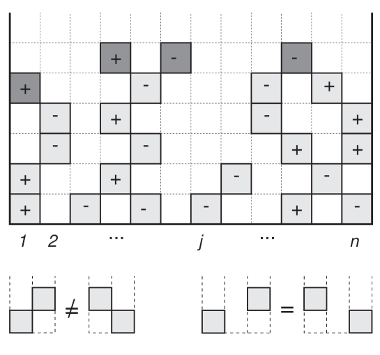
Figure 3: Typical configuration of a colored heap. Elements of a roof are shown by filled squares.

Namely, we consider the strip $P={\bf n}\times{{\sf Z\kern-3.20007ptZ}}^{+}\subset{{\sf Z\kern-3.20007ptZ}}^{2}\;\left({\bf n}=\{1,2,...,n\};{{\sf Z\kern-3.20007ptZ}}^{+}=\{0,1,...,\}\right)$ as a subset of the lattice ${{\sf Z\kern-3.20007ptZ}}^{2}$.

Definition 7

I. We call as a heap the finite set $S\in P$, satisfying the conditions:

1) In a horizontal line the cells from the set $S$ can not be neighbors;

2) Each cell from $S$, not standing in the first horizontal line has at least one cell in the previous horizontal line, touching it. (The touching of cells means that the horizontal coordinates of such cells differ not more, than by 1.)

II. Let each cell from $S$ has two colors $(+,-)$. We shall assume, that besides the conditions 1 and 2 the following one is fulfiled:

3) In one and the same vertical row $i=1,...,n$ the cells of different color can not be the neighbors.

In the last case $S$ refers to as a colored heap.

The set of heaps with number of cells $K\geq 0$ is denoted by $H_{K}^{(n)}$ (while $H^{(n)}=\mathop{\cup}\limits_{K=0}^{\infty}H_{K}^{(n)}$ ($H_{0}^{(n)}$ is an empty heap). The concept of a heap had been introduced and investigated by Viennot [Vi] in connection with combinatoric problems of partially commutative monoids of Cartier and Foata [CF] and so-called ”directed lattice animals” considered in [HNDV, Vi]. Denote by $CH_{K}^{(n)}$ the set of colored heaps with the number of cells $K\geq 0$, thus $CH^{(n)}=\mathop{\cup}\limits_{K=0}^{\infty}CH_{K}^{(n)}$. As far as we know, the colored heaps have not been considered so far.

Definition 8

The numbered heap is a heap, whose cells are enumerated by natural numbers so, that the the enumeration is monotone, i.e. if two cells touch each others, the top cell has larger number.

Lemma 3

There exists a bijection $\tau$ between the set of words of a locally free group ${\cal LF}_{n}$ and the set of colored heaps $CH^{(n)}$, for which the one-to-one correspondence between the elements (words) of ${\cal LF}_{n}$ and colored heaps $CH^{(n)}$ is established.

For the semi–group ${\cal LF}_{n}^{+}$ the same statement is true with the replacement $CH^{(n)}\to H^{(n)}$ and for this case the interpretation was given in the work [Vi].

Proof. By induction. The unity of the group corresponds to an empty heap. Let $\tau$ be determined for words of length $\leq K$. Compare to a word of length $K+1$ a colored heap, which is received by adding the element $g_{i}^{\pm 1}$ in an $i$’s vertical row to already existing colored heap, i.e. put a cell so, that the conditions 1 and 2 of Lemma 3 are satisfied. If directly under a new cell there was already a cell with the same coordinate $i$ and the opposite color, these cells cancel. It is easy to see, that if two words are equal, the corresponding (colored) heaps coincide.

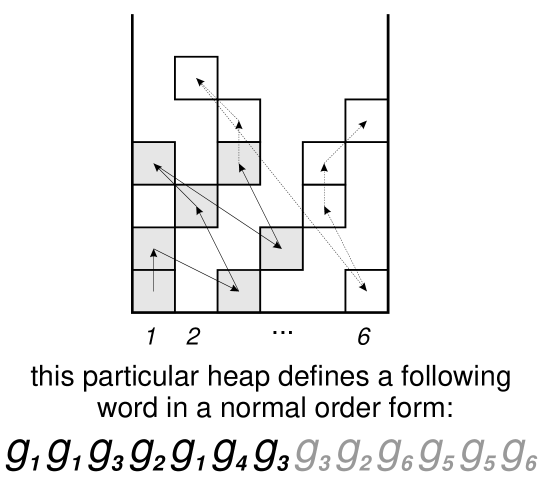
Figure 4: Example of construction of normally ordered word by given heap. The configuration of some current cluster is shown by filled cells.

Let us show now that any (colored) numbered heap is uniquely associated with some word in ${\cal LF}_{n}$. Namely, we construct an algorithm which sets a word in the normal order by some numbered (colored) heap:

1. Denote the most left–hand cell at bottom as the cell No.1 corresponding to the first letter in the normal order form for a given heap. For definiteness assume that this cell is disposed in a $j$’s column. The cell No.2 is a cell located in a column $k$ ($k\leq j$) as close as possible to the cell No.1. Now we search for cells left–most close to cell No.2 and so on… Continuing such enumeration we get a part of a heap called ”cluster”.

2. If there are no more cells satisfying the rule 1, we continue numbering with the most bottom cell which is closest right–hand neighbor to the given cluster such that this new cell leaves the roof of the cluster without changes. This new cell is added to the cluster and enumeration is continued recursively.

As a result get numbering corresponding the normal form of a given word. Thus, Lemma 3 is proved.  

Remark 3

There is an analogy between heaps and Young diagrams, as well as between numbered heaps and Young tables [Ve2].

Dynamics of the words’ growth, i.e. the random walk on ${\cal LF}_{n}$ (${\cal LF}_{n}^{+}$) acquires a following obvious geometrical sense: it is a Markov chain with the states taken from the set of colored heaps (or just heaps). The transitions consist in addition of cells (in a view of conditions 1–3 of the Definition 7) with the probabilities $\frac{1}{2n}$ for ${\cal LF}_{n}$ and $\frac{1}{n}$ for ${\cal LF}_{n}^{+}$.

For each element $w$ of the locally free group ${\cal LF}_{n}$, written in the normal form we define the set of achievable generators $T(w)$ (see [DN2]):

$$T(w)=\left\{i=1,...,n:K(w\,g_{i})=K(w)-1\right\}$$

where $K(w)$ is the word’s length.

Achievable generator $g_{i}$ in the word $w$ refers to as such generator in the representation $w=w_{1}\,g_{i}^{m}\,w_{2}$, that at multiplication of the element $w$ from the right hand side by $g_{i}^{\pm 1}$, the new word $w^{\prime}$ can be recorded as $w^{\prime}=w_{1}\,g_{i}^{m\pm 1}\,w_{2}$, i.e. $w_{2}$ and $g_{i}$ commute. In particular, the generator $g_{i}^{m\pm 1}$ can be reduced, if $m\pm 1=0$. It is easy to realize that achievable generators are such, that can be reduced in one step of a random walk. Further we shall number generators $g_{i}$ by the index $i$, and generators $g_{i}^{-1}$ by the index $-i$.

The set $T(w)$ has following obvious properties:

(i) If $i\in T(w)$, then $-i\notin T(w)$ and if $-i\in T(w)$ then $i\notin T(w)$;

(ii) If $i\in T(w)$ or $-i\in T(w)$ then $\pm(i-1),\pm(i+1)\notin T(w)$.

The last property entails the inequality $\#T(w)\leq\left[\frac{n+1}{2}\right]$.

We continue the geometric interpretation of concepts and give the visual description of the set $T(w)$ of achievable elements.

Definition 9

We call as the roof of the heap (of the colored heap) the set $T(S)$ of those elements of a heap which have no upper neighbors in the same and closest vertical rows.

In other words, some element belongs to the roof of the heap of $K$ elements if after the removal of this element we get the heap of $K-1$ elements.

Remark 4

In continuation of the similarity of heaps and Young diagrams, we can say that the roof is analogous to the corners of the Young diagrams.

4.1 Mathematical expectation of the heap’s roof

In a geometrical interpretation described above the set $T(S)$ of achievable elements is a set of such cells of a heap, removing of which for one step leaves a configuration allowable (see the Definition 9).

The roof’s basis of a heap $S$ is the subset $T(S)=\{1,...,n\}$ of the numbers of achievable generators. This subset, as it can be seen from the properties (i)–(ii), satisfies the condition: if $(k_{1},k_{2})\in T(S)$ then $|k_{1}-k_{2}|>1$. Denote by ${\cal T}_{n}$ the family of all such subsets of the set $\{1,...,n\}$. In case of a colored heap the basis consists of the painted in two colors $(+,-)$ subsets of $\{1,...,n\}$. We denote these subsets by ${\cal T}_{n}^{c}$.

Remark 5

Let $w$ be the element of the group ${\cal LF}_{n}$ and $S$ be the corresponding heap. Then $T_{n}(S)$ is exactly the set of achievable generators.

It is convenient to characterize ${\cal T}_{n}$ by a vector $(\varepsilon_{1},...,\varepsilon_{n})$ with elements 0 and 1, where $\{\varepsilon_{r}=1\}\Leftrightarrow r\in T$.

Lemma 4

The power of the set ${\cal T}_{n}$ is equal to the Fibonacci number $F_{n}$ and hence it grows as $\lambda^{n}$, where $\lambda=\frac{\sqrt{5}+1}{2}\approx 1.618$ is the golden mean. The power of the set ${\cal T}_{n}^{c}$ is equal to $2^{n}$.

Proof. The power of the set ${\cal T}_{n}$ is equal to the number of sequences of elements $0$ and $1$ of length $n$, such that these sequences have not the elements $1$ in succession, i.e. satisfy the recursion relation

$$\begin{array}[]{l}F_{n}=F_{n-1}+F_{n-2}\vskip 6.0pt plus 2.0pt minus 2.0pt\\ F_{1}=1;F_{2}=2,\end{array}$$ (30)

which defines the Fibonacci sequence.

Similarly, the number of the elements of the set ${\cal T}_{n}^{c}$ satisfies the recursion relation

$$\begin{array}[]{l}F_{n}^{c}=F_{n-1}^{c}+2F_{n-2}^{c}\vskip 6.0pt plus 2.0pt minus 2.0pt\\ F_{0}^{c}=1;F_{1}^{c}=2;F_{2}^{c}=4\end{array}$$ (31)

Actually, if the sequence ${\cal T}_{n}^{c}\subset F_{n}^{c}$ begins with 0, the part remaining after removal of 0 is any sequence from $F_{n-1}^{c}$. If ${\cal T}_{n}^{c}$ begins with $1$, then by definition the 2nd element is 0. Deleting these two elements (1 and following after it 0), we get a sequence from $F_{n-2}^{c}$, Thus, the power of the set ${\cal T}_{n}^{c}$ satisfies recursion relation (31), and consequently $F_{n}^{c}=2^{n}$.  

Define the time–homogeneous Markov chain, the set of states of which in any moment of a time are the sets $T\in{\cal T}$ and the transition probabilities from the state $T$ to the state $T^{\prime}$ are determined by the time–independent rules. Let $T=\{\varepsilon_{1},...,\varepsilon_{n}\};\;T^{\prime}=\{\varepsilon^{\prime}_{1},...,\varepsilon^{\prime}_{n}\}$. Then the transition matrix is as follows. The transition probability $T\to T^{\prime}$ is nonzero and is equal to $\frac{1}{n}$ only for the cases when $\varepsilon_{i}=\varepsilon^{\prime}_{i}$ for all $i$ except not more than three consecutive numbers, say $(\varepsilon_{r-1},\varepsilon_{r},\varepsilon_{r+1})$ and $(\varepsilon^{\prime}_{r-1},\varepsilon^{\prime}_{r},\varepsilon^{\prime}_{r+1})$ and for these triples one of the following conditions is satisfied:

$$\begin{array}[]{ll}\mbox{If $\varepsilon_{r-1}=\varepsilon_{r+1}=1$}&\mbox{then $\varepsilon^{\prime}_{r}=1,\varepsilon^{\prime}_{r-1}=\varepsilon^{\prime}_{r+1}=0$;}\vskip 6.0pt plus 2.0pt minus 2.0pt\\ \mbox{If $\varepsilon_{r-1}=1,\varepsilon_{r+1}=0$}&\mbox{then $\varepsilon^{\prime}_{r}=1;\varepsilon^{\prime}_{r-1}=\varepsilon^{\prime}_{r+1}=0$;}\vskip 6.0pt plus 2.0pt minus 2.0pt\\ \mbox{If $\varepsilon_{r+1}=1,\varepsilon_{r-1}=0$}&\mbox{then $\varepsilon^{\prime}_{r}=1;\varepsilon^{\prime}_{r-1}=\varepsilon^{\prime}_{r+1}=0$;}\vskip 6.0pt plus 2.0pt minus 2.0pt\\ \mbox{If $\varepsilon_{r-1}=\varepsilon_{r}=\varepsilon_{r+1}=0$}&\mbox{then $\varepsilon^{\prime}_{r-1}=\varepsilon^{\prime}_{r+1}=0,\varepsilon^{\prime}_{r}=1$.}\end{array}$$ (32)

Thus, the Markov chain is determined on the set of states ${\cal T}_{n}$.

Later on we will be interested in the asymptotics of a mathematical expectation of the size of a roof following the outline of the paper [DN2].

Theorem 2

The limit of the mathematical expectation of the number of achievable generators for a random walk on the semi–group ${\cal LF}_{n}^{+}$ for $n\gg 1$ (i.e. the limit of the mathematical expectation of the roof of the heap) is

$$\lim_{N\to\infty}E\#T(w_{N})=\frac{n}{3}$$ (33)

Proof. Compute the mathematical expectation of a number of removable (achievable) elements when we do not distinguish between generators and their inverses, i.e. for the random walk on the semi–group ${\cal LF}_{n}^{+}$.

Represent the elements of the roof $T(w)$ (i.e. the number of achievable generators) graphically by filled boxes on the diagram as it is shown below:

Here $n=11,\;\#T=4$.

Denote by $h_{j}=k_{j}-k_{j-1}-1$ the number of intervals of lengths $j$ between neighboring boxes or between a box and the edge of the diagram.

Let $T$ consists of the set $\{k_{1},...,k_{s}\}$. If the edge points $(1$ and $n)$ do not belong to $T$, then $h_{1}=k_{1},\;h_{s+1}=n-k_{s}-1$; if one or both edge points belong to $T$, then $h_{1}=k_{1}-1,\;h_{s+1}=n-k_{s}$. For example, if $k_{1}=1$ then $h_{1}=0$, or if $k_{s}=n$ then $h_{s}=0$. (On the above diagram $h_{1}=0,\,h_{2}=1,\,h_{3}=3,\,h_{4}=1$). The numbers $h_{j}$ satisfy the following relation, valid under neglecting the ”boundary effects” at $\#T\gg 1,\;n\gg 1$:

$$\sum_{j}h_{j}=n-\#T$$ (34)

It is not hard to establish the rules according to which the diagram is changed at such multiplication of $w$ by $g_{r}$ (or by $g_{r}^{-1}$), which increases $\#T(w)$ by $1$: in $r$’s position appears a point while in positions $(r-1)$ and/or $(r+1)$ the points (which were present) disappear. Having in mind this rule, let us write the explicit expressions for the 1–step increment of a roof’s length, $\Delta T(w)$, expressing it in terms of $h_{j}(w)$ provided that the boundary points do not belong to $T$:

$$\left\{\begin{array}[]{ll}\Delta T(w)=+1&\mbox{with the probability $\frac{1}{n}\sum\limits_{j:h_{j}\geq 3}(h_{j}-2)$}\vskip 6.0pt plus 2.0pt minus 2.0pt\\ \Delta T(w)=0&\mbox{with the probability $\frac{1}{n}\left(\#T+2\#\{j:h_{j}\geq 2\}\right)$}\vskip 6.0pt plus 2.0pt minus 2.0pt\\ \Delta T(w)=-1&\mbox{with the probability $\frac{1}{n}\#\{j:h_{j}=1\}$}\end{array}\right.$$ (35)

Summing (35), we obtain the conditional mathematical expectation of the conditional probability of local reconstruction of a roof for the fixed element $w$:

$$\begin{array}[]{lll}E_{w}\Delta T&=&1\cdot\frac{1}{n}\sum\limits_{j:h_{j}\geq 3}(h_{j}-2)+0\cdot\left(\#T+\frac{2}{n}\#\{j:h_{j}\geq 2\}\right)+(-1)\cdot\frac{1}{n}\#\{j:h_{j}=1\}\\ &=&\frac{1}{n}\sum\limits_{j}(h_{j}-2)=\frac{1}{n}\sum\limits_{j}h_{j}-\frac{2}{n}\#T=1-\frac{3}{n}\#T(w)\end{array}$$ (36)

Let us mention that depending on whether the boundary points belong or do not belong to the set $T(w)$, the right–hand side of Eq.(36) is changed by terms which do not exceed than $\frac{4}{n}$. Therefore in the large $n$ limit the expression (36) is exact. In case of periodic boundary conditions Eq.(36) is exact for any finite values of $n$.

As far as our Markov chain has finite set of states and is ergodic, it has the unique invariant measure. The Markov chain with this invariant measure is stationary. So, the mathematical expectation $E[\Delta T(w)]$ over all elements $w$ with respect to the invariant measure exists and is finite, therefore $E[\Delta T(w)]=0$. Thus, from the strong law of large numbers (or, equivalently, from the individual ergodic theorem) it follows that for the random walk on the semi–group we have Eq.(33) for the mathematical expectation of the number of achievable elements (i.e. the set of elements of the roof’s elements).  

Consider now the case of the group ${\cal LF}_{n}$. The distinction between the semi–group ${\cal LF}_{n}^{+}$ (i.e. the heap) and the group ${\cal LF}_{n}$ (i.e. the colored heap) is due to the fact that for the random walk on the group it is possible to reduce the word with the probability $\frac{1}{2n}$. To account for that, we introduce the probabilities $p_{w}^{+}$ and $p_{w}^{-}$ to increase and to reduce the size of the roof $\#T(w)$ per unity under the condition of the word’s length reduction. The mathematical expectation is a difference of conditional probabilities $p_{w}^{+}$ and $p_{w}^{-}$ to change the value $\#T(w)$ per unity provided that reduction of a word occurs. This difference should be added to the mathematical expectation of the change of $\#T(w)$ in case of semi–group (32):

$$E_{w}\Delta T=1-\frac{3}{n}\#T(w)+\frac{p_{w}^{+}-p_{w}^{-}}{2n}\#T(w).$$ (37)

That gives (compare to (32)–(33))

$$E\#T=\frac{n}{3-\frac{1}{2}(p^{+}-p^{-})}=\frac{n}{3-\alpha}$$ (38)

where $p^{+}=Ep_{w}^{+};\;p^{-}=Ep_{w}^{-};$ and $\alpha=\frac{1}{2}(p^{+}-p^{-})$.

On can easily realize that for some configurations of heaps $w$ we could have $p^{+}-p^{-}\neq 0$ and in these cases the mathematical expectation $E_{w}\Delta T$ for the group (colored heap) and for the semi–group (heap) do not coincide. However, we believe, that at $N\to\infty$ (i.e. in a stationary mode) $Ep_{w}^{+}=Ep_{w}^{-}$ and the following hypothesis (expressed first by J. Desbois in [DN2]) is valid:

Conjecture 1

The mathematical expectation of a roof (a set of achievable elements) for the heap (the locally free semi–group ${\cal LF}_{n}^{+}$) and for the colored heap (the locally free group ${\cal LF}_{n}$) coincide at $n\gg 1$. Hence,

$$\lim_{N\to\infty}E\#T(w_{N})=\frac{n}{3}$$ (39)

The concept of a roof is the same for the heap (the semi–group) and for the colored heap (the group), however the dynamics determined in these two cases is distinct.

The random walk on the locally free semi–group (group) has been reduced to a Markov dynamics of heaps (colored heaps). We have defined a new dynamics—the dynamics of the roofs, Markovian in the case of semi–group, by which the general dynamics is restored and which is convenient for computations. In the case of the group this dynamics is not Markovian anymore, but nevertheless enables to get some nontrivial estimates.

4.2 Drift as mathematical expectation of number of cells in the heap

Let us compute now the change of a length of some fixed word $w$ for a random walk on a group ${\cal LF}_{n}$. It is obvious, that for one step of the random walk the length of a word can change by $\pm 1$. The multiplication by a given generator, or by its inverse, occurs with the probability $\frac{1}{2n}$ and thus, the conditional mathematical expectation $E(w)$ to change a word’s length is determined for a fixed element $w$. Below we shall compute $E(w)$ and shall be convinced, that the answer depends only on a size of a roof, i.e. on a size of a set $\#T(w)$ of achievable generators $T(w)$.

Consider a fixed element $w$ of the group ${\cal LF}_{n}$ such that the set of achievable generators $w$ is $\{1\leq k_{1}<k_{2}<...<k_{s}<n\}$. Assume that with the probability $\frac{1}{2n}$ the word $w$ is multiplied by a generator $g_{r}$ or $g_{r}^{-1}$ (for definiteness let us choose $g_{r}$). Denote the set of achievable generators of the element $w^{\prime}=w\;g_{r}$ as $T^{\prime}\equiv T(w^{\prime})$. Then the dynamics of the change of the set $T(w)$ is settled by the following opportunities (compare to the above relations (32)):

We have the following possibilities:

I. Provided that the the word is increased, i.e. $K^{\prime}(wg_{i})=K(w)+1$ the dynamics of the roof is described by the relations (32) valid for the semigroup ${\cal LF}_{n}^{+}$;

II. Provided that the word is reduced, i.e. $K^{\prime}(wg_{i})=K(w)-1$, we have:

$$\begin{array}[]{ll}\mbox{If $\varepsilon_{r}=1$}&\mbox{then ${\cal T}\to{\cal T}^{\prime}\equiv{\cal T}^{-}$}\end{array}$$ (40)

where ${\cal T}^{-}$ is the roof’s configuration obtained by the cancellation of one of the element of the roof ${\cal T}$ located in position $r$. (This rule cannot be described in local terms).

The probability of a word’s length reduction is $\frac{\#T}{2n}$, because for each element of a roof there is a unique possibility to be reduced if and only if at the following step the element inverse to the former one has arrived. Accordingly, the probability to increase of a word’s length is $1-\frac{\#T}{2n}$, what follows from the possibility mentioned above to change a word’s length for one step by $\pm 1$. As a result, the mathematical expectation of the total change of a word’s length for one step of random walk on the group ${\cal LF}_{n}$ is

$$E_{g_{r}}[K(w)-K(w\;g_{r})]=-\frac{E\#T(w)}{2n}+\left(1-\frac{E\#T(w)}{2n}\right)=1-\frac{E\#T(w)}{n}$$ (41)

The indicated computation proves the following Lemma:

Lemma 5

The conditional mathematical expectation of the word’s length $K(w)$ after $N$ steps of the random walk on the group ${\cal LF}_{n}$ for the fixed last element $w$ is

$$E_{w}K=N\left(1-\frac{E\#T(w)}{n}\right)$$

hence the drift (i.e. the mathematical expectation of a normalized words’ length) is

$$l=\lim_{N\to\infty}\frac{1}{N}E_{w}K=1-\frac{E\#T(w)}{n}$$

Thus, for calculation of the drift it is sufficient to know the mathematical expectation $E\#T(w)$ of the roof—see Eq.(37).

Theorem 3

The mathematical expectation of the drift of a random walk on a locally free group at $n\gg 1$ is

$$l=1-\frac{E\#T(w)}{n}=1-\frac{1}{3-\alpha}=\frac{2-\alpha}{3-\alpha}$$ (42)

where $\alpha$ is defined in (38).

Conjecture 2

The mathematical expectation of the drift on the locally free group at $n\gg 1$ is

$$l=\frac{2}{3}$$ (43)

The Conjecture 2 is a direct consequence of the Conjecture 1 (J. Desbois in [DN2]) but still it is not proved rigorously.

5 Random walk on locally free group: entropy

Let us remind, that the entropy $h$ of the random walk on the group $G$ according to the theorem similar to the Shannon’s one and proved in [Ve2, VKai, Av, De] can be represented as follows (see the Definition 6):

$$H(w)=-\lim_{N\to\infty}\frac{1}{N}\log\mu^{N}(g^{N}),$$

where $w=g^{N}$; the limit in a right hand side is identical for almost all trajectories $\{g^{N}\}_{N=1}^{\infty}$; $N$ is the number of the random walk steps (i.e. the nonreduced word’s length); $\mu^{N}$ is the $N$–time convolution of a measure $\mu$.

In turn, the value of a measure $\mu^{N}$ on the words $w$ with $n$ generators can be written in the following form

$$\mu^{N}(w)=\frac{\#{\cal L}(w)}{n^{N}}$$ (44)

where $\#{\cal L}(w)$ is the number of various (dynamic) representations of the element $w$ by words of length $N$ in the framing $\{g_{1},...,g_{n},g_{1}^{-1},...,g_{n}^{-1}\}$. The value $\#{\cal L}(w)$ is the number of different ways on the Cayley graph of the group, leading from the root point of the graph (the unity of the group).

It is convenient to divide the problem of computation of the entropy of the random walk on a group ${\cal LF}_{n}$ in two parts and to begin with the case of the semi–group ${\cal LF}_{n}^{+}$, while for the group ${\cal LF}_{n}$ the result will be the straightforward generalization of the corresponding results for the semi–group ${\cal LF}_{n}^{+}$.

5.1 Entropy of random walk on semi–group ${\cal LF}_{n}^{+}$

As it has been found in the previous section during the study of the drift, the dynamics of the increments of words (i.e. dynamics of the heap $S$) for the random uniform addition of cells is uniquely determined by the dynamics of the roof $T$ of the heap $H$. Moreover, we have found (see Eq.(33)), that in the limit $N\to\infty$ and at $n\gg 1$ the mathematical expectation of the roof’s size $E\#T$, normalized by $n$ (i.e. the mathematical expectation of the density of achievable elements) is $1/3$.

Let us prove the Lemma:

Lemma 6

The fluctuations of mathematical expectation of the roof for $n\gg 1$ have the asymptotic behavior

$$\frac{E\left|\#T^{2}-E(\#T)^{2}\right|}{E(\#T)^{2}}\leq\frac{{\rm const}}{n}$$

where we have denoted

$$E\#T\equiv\lim_{N\to\infty}E\#T(w_{N})$$

Proof. Rewrite (33) in the form

$$E(\#T)^{2}\equiv\left[\lim_{N\to\infty}E\#T(w_{N})\right]^{2}=\frac{n^{2}}{9}$$ (45)

Using Eqs.(35)–(36) for the probabilities of local rearrangements of the roof we get the mathematical expectation of the roof’s fluctuations:

$$\begin{array}[]{lll}E\Delta(\#T^{2})&=&E\Delta\Big{[}(\#T^{\prime})^{2}-(\#T)^{2}\Big{]}\vskip 6.0pt plus 2.0pt minus 2.0pt\\ &=&1\cdot q_{+}\Big{(}(\#T)^{2}-(\#T-1)^{2}\Big{)}+0\cdot q_{0}+(-1)\cdot q_{-}\Big{(}(\#T+1)^{2}-(\#T)^{2}\Big{)}\vskip 6.0pt plus 2.0pt minus 2.0pt\\ &=&2(q_{+}-q_{-})\#T-(q_{+}+q_{-})\end{array}$$ (46)

where

$$q_{+}=\frac{1}{n}\sum_{j:h_{j}\geq 3}(h_{j}-2);\quad q_{0}=\frac{1}{n}\left(\#T+2\#\{j:h_{j}\geq 2\}\right);\quad q_{-}=\frac{1}{n}\#\{j:h_{j}=1\}$$

Taking into account, that $q_{+}-q_{-}=1-\frac{3}{n}\#T$, we obtain from (46):

$$E\Delta(\#T^{2})=E\left\{2\left(1-\frac{3}{n}\#T\right)\#T-(q_{+}+q_{-})\right\}$$ (47)

For the invariant initial distribution it should be $E\Delta(\#T^{2})=0$, therefore the mathematical expectation of a square of the roof’s size can be received from the following relation

$$E\Delta(\#T^{2})=2E\#T-\frac{6}{n}E(\#T)^{2}-E(q_{+}+q_{-})=0$$

whence we get

$$E(\#T)^{2}=\frac{n}{3}E\#T-\frac{n}{6}E(q_{+}+q_{-})$$

Estimating the mathematical expectation from above as $E(q_{+}+q_{-})<{\rm const}$, we arrive at the equation:

$$E(\#T)^{2}=\frac{n^{2}}{9}-\frac{{\rm const}\,n}{6}=\frac{n^{2}}{9}+o(n^{2})$$

Comparing the last expression with (45), we get the statement of Lemma 6.  

Theorem 4

The entropy of the random walk on the locally free semi–group ${\cal LF}_{n}^{+}$ for $n\gg 1$ is

$$h=\log 3+O(n^{-1})$$ (48)

Proof. Write the recursion relation of the change of the value $\#{\cal L}(w)$ (see Eq.(44) at exception of one fixed cell of a roof, where $w$ there is the element of the group, possessing at least one representation by words of length $N$. Let $\#{\cal L}(w)$ and $\#{\cal L}(w\setminus g_{i})$ ($i\in T$) be the numbers of various representations of the elements $w=g^{N}$ and $w^{\prime}=g^{N}\setminus g_{i}$ correspondingly. Then is fair the recursion relation

$$\#{\cal L}(g^{N})=\sum_{g_{i}\in T}\#{\cal L}(g^{N}\setminus g_{i})$$ (49)

where the sum is taken over all elements $g_{i}$ from the roof $T$.

Thus our problem is reduced to account for the number of representations of a group element by generators in course of a random walk.

Using the definition (44) and Eq.(49) we can write:

$$-\frac{1}{N}\log\mu^{N}(g^{N})=-\frac{1}{N}\log\frac{\#{\cal L}(g^{N})}{n^{N}}$$ (50)

Taking into account that the number of roofs of a given shape is equal to the chronological (”time–ordered”) multiplication of the roofs’ lengths, we arrive at the following equation:

$$-\frac{1}{N}\log\frac{\#{\cal L}(g^{N})}{n^{N}}=-\frac{1}{N}\log\frac{\displaystyle\prod_{j=1}^{N}\#T_{j}}{n^{N}}=-\frac{1}{N}\sum_{j=1}^{N}\log\frac{\#T_{j}}{n}$$ (51)

Defining the new variable

$$\xi_{j}=\frac{3\#T_{j}}{n}-1$$

we can rewrite (51) in the form

$$\begin{array}[]{c}\displaystyle\lim_{N\to\infty}-\frac{1}{N}\sum_{j=1}^{N}\log\frac{1+\xi_{j}}{3}=\log 3-\lim_{N\to\infty}\frac{1}{N}\sum_{j=1}^{N}\log(1+\xi_{j})=\log 3-\lim_{N\to\infty}E\log(1+\xi_{N})\\ \displaystyle\leq\log 3-\lim_{N\to\infty}E\xi_{N}+\lim_{N\to\infty}\frac{1}{2}E\xi_{N}^{2}\end{array}$$ (52)

where

$$\begin{array}[]{l}\displaystyle\lim_{N\to\infty}E\xi_{N}\equiv E\xi=\frac{3}{n}E\#T\\ \displaystyle\lim_{N\to\infty}E\xi_{N}^{2}\equiv E\xi^{2}=\frac{9}{n^{2}}E\#T^{2}-\frac{6}{n}E\#T+1,\end{array}$$

while $E\#T$ and $E\#T^{2}$ are the limits (for $N\to\infty$) of the mathematical expectations of the roof’s size $\#T$ and of its square $\#T^{2}$ for fixed value of $n$.

The statement of Lemma 6 can be rewritten as

$$\frac{E\left|\#T^{2}-\frac{n^{2}}{9}\right|}{\frac{n^{2}}{9}}=E\left(\frac{3\#T}{n}\right)^{2}-1\leq\frac{{\rm const}}{n}$$

and in terms of the variable $\xi=\frac{3\#T}{n}-1$ the last inequality reads

$$E(\xi+1)^{2}-1\leq\frac{{\rm const}}{n}.$$

Using the fact that $E\xi=0$ we arrive at the conclusion that for $n\gg 1$

$$E\xi^{2}\leq\frac{{\rm const}}{n}$$ (53)

Substituting (52) for the estimate (53) we get the desired statement of the Theorem:

$$h=\displaystyle-\lim_{N\to\infty}\frac{1}{N}\,\log\mu^{N}(g^{N})=\log 3+O(n^{-1})$$ (54)

what completes the proof.  

Theorem 5

For the random walk on the locally free semi–group ${\cal LF}_{n}^{+}$ the logarithmic volume $v$, the drift $l$ and the entropy $h$ satisfy at $n\gg 1$ the strict inequality

$$v\,l>h$$

where $v\equiv v({\cal LF}_{n}^{+});\;l\equiv l({\cal LF}_{n}^{+});\;h\equiv h({\cal LF}_{n}^{+})$.

Proof.

(i) From the Corrolary 2 of the Theorem 1 we have

$$v({\cal LF}_{n}^{+})\to\log 4$$

(ii) The drift of the random walk on ${\cal LF}_{n}^{+}$ is strictly equal to 1, i.e.

$$l=1$$

(iii) By Theorem 4 we have

$$h({\cal LF}_{n}^{+})\to\log 3$$

Comparing the values of $v$, $l$ and $h$, we get the strict inequality $v>h$ for the random walk on ${\cal LF}_{n}^{+}$.  

5.2 Entropy of random walk on group ${\cal LF}_{n}$

Theorem 6

The entropy of the random walk on the locally free group ${\cal LF}_{n}$ at $n\gg 1$ is

$$h=\log(3-\alpha)+O(n^{-1})$$ (55)

where $\alpha=\frac{1}{2}(p^{+}-p^{-})$ (see 38).

Proof. In the case of the group the exact value of $E\#T$ is unknown as far as $E\#T$ contains some unknown value $\alpha=\frac{1}{2}(Ep_{w}^{+}-Ep_{w}^{-})$. Remind that $p_{w}^{+}$ and $p_{w}^{-}$ are the probabilities of the change of the value $\#T(w)$ by $\pm 1$ provided the reduction of a word (see Eq.(38)). Nevertheless, we can follow directly the outline of the proof of the Theorem 4 with just a single replacement $\xi_{j}\to\xi_{j}-\alpha$. As a result, in the limit $n\gg 1$ we get (55).  

For the group ${\cal LF}_{n}$ as well as in case of semi–group ${\cal LF}_{n}^{+}$, the entropy $h$ and the drift $l$ of the random walk are determined by the mathematical expectation of the roof’s size $E\#T$. Nevertheless in case of the group the numerical value of the mathematical expectation of a colored heap’s roof depends on the value $\alpha$. However as far as our purpose is to prove that for locally free group in the limit of infinite number of generators the strict inequality $l\,v<h$ holds, it is sufficient to estimate appropriately the interval of change of $\alpha$.

Theorem 7

For the random walk on the locally free group ${\cal LF}_{n}^{+}$, the logarithmic volume $v$, the drift $l$ and the entropy $h$ satisfy at $n\gg 1$ the strict inequality

$$v\;l>h$$

where $v\equiv v({\cal LF}_{n});\;l\equiv l({\cal LF}_{n});\;h\equiv h({\cal LF}_{n})$.

Proof. For the proof we shall use again the statements of the Theorems 1, 3, and 4.

(i) By the Theorem 1:

$$v({\cal LF}_{n})\to\log 7$$ (56)

(ii) By the Theorem 3:

$$l({\cal LF}_{n})\to\frac{2-\alpha}{3-\alpha},$$ (57)

(iii) By the Theorem 4:

$$h({\cal LF}_{n})\to\log(3-\alpha).$$ (58)

By definition $\alpha=\frac{1}{2}(p^{+}-p^{-})$. Because $p^{+}+p^{-}=1$, the following estimate is valid $|\alpha|<\frac{1}{2}$. Thus, the values of the drift and the entropy lie within the interval

$$\frac{3}{5}<l<\frac{5}{7}$$

and

$$\log\frac{5}{2}<h<\log\frac{7}{2}$$

Define the discrepancy $\varepsilon=l\,v-h$ and check that $\varepsilon(\alpha)>0$ for all values of $|\alpha|$ from the interval $|\alpha|<\frac{1}{2}$. Consider the function

$$\varepsilon(\alpha)=\frac{2-\alpha}{3-\alpha}\log 7-\log(3-\alpha)$$

Computing the derivative $\frac{d\varepsilon(\alpha)}{d\alpha}$, one can easily verify that on the interval $-\frac{1}{2}<\alpha<\frac{1}{2}$ the function $\varepsilon(\alpha)$ is strictly positive, hence $l\,v-h>0$. The Theorem is proved.  

6 Conclusion

Let us outline the applications of the results received above to the braid groups and semi–groups.

6.1 Some remarks about the relations to braid groups and semi–groups

As it has been mentioned already, the braid group $B_{n}$ is the factor–group of the locally free group ${\cal LF}_{n}$ and simultaneously, ${\cal LF}_{n}$ is the subgroup of $B_{n}$. The same relations are valid for the semi–group of positive braids $B_{n}^{+}$ and the locally free semi–group ${\cal LF}_{n}^{+}$.

From here, as well as from the Consequence 1 of Lemma 1 and Theorem 1, immediately follows the Theorem:

Theorem 8

The logarithmic volumes $v(B_{n})$ and $v(B_{n}^{+})$ for $n\gg 1$ satisfy the bilateral estimates

$$\begin{array}[]{l}\frac{1}{2}\log 7<v(B_{n})\leq\log 7\vskip 6.0pt plus 2.0pt minus 2.0pt\\ \log 2<v(B_{n}^{+})\leq\log 4\vskip 6.0pt plus 2.0pt minus 2.0pt\end{array}$$ (59)

Proof. The estimate from above is a direct consequence of the fact that $B_{n}$ is the factor–group of the locally free group ${\cal LF}_{n}$. Thus,

$$v_{B_{n}}\leq v_{{\cal LF}_{n}}\equiv\log 7$$

In order to obtain the estimate from below let us notice that the embedding $\rho_{n}$ of ${\cal LF}_{n}$ in $B_{n}$ and of ${\cal LF}_{n}^{+}$ in $B_{n}^{+}$ is realized via the identity $f_{i}\to\sigma_{i}^{2}$. Thus, in the case of the group we have:

$$V(\rho_{n}:\,{\cal LF}_{n},K)\subset V(B_{n},2K)$$

and

$$\frac{\log V(\rho_{n}\;{\cal LF}_{n},K)}{K}\leq\frac{V(B_{n},2K)}{K},$$

hence

$$v_{{\cal LF}_{n}}\equiv\log 7\leq 2v_{B_{n}}$$

therefore

$$\frac{1}{2}v_{{\cal LF}_{n}}\leq v_{B_{n}},$$

Along the same line the case of the semi–group ${\cal LF}_{n}^{+}$ can be treated.  

Apparently, the upper estimate in Eq.(59) is closer to the true value, than the lower one.

Theorem 9

The drift $l(B_{n})$ on the braid group $B_{n}$ at $n\gg 1$ satisfies the inequality

$$\frac{2-\alpha}{2(3-\alpha)}<l(B_{n})\leq\frac{2-\alpha}{3-\alpha}$$ (60)

Proof. The bilateral estimate (60) is also a direct consequence of the fact that the the braid group is the factor–group of the locally free group and in turn the locally free group is the subgroup of the braid group. The value $\alpha$ has been defined above and varies in the interval $-\frac{1}{2}<\alpha<\frac{1}{2}$.  

For the entropy of the random walk on the braid group the corresponding bilateral estimates have not yet received.

6.2 Physical interpretation of results

Let us discuss briefly the physical sense of a strict inequality $lv>h$ for the locally free group and for the ballistic deposition process—see fig.5.

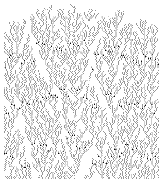
Figure 5: Typical configuration obtained in numerical simulations of the uniform heap’s growth.

The relation (44) permits one to estimate the number of various dynamic representations of almost all (typical) elements $w$ by words of length $N$ with respect to the uniform measure $\mu$:

$$\#{\cal L}(w)\approx\exp(Nh)$$

that for locally free group gives with the exponential accuracy

$$\#{\cal L}(w)\approx(3-\alpha)^{N}$$

Thus as stated already, the value $\#{\cal L}(w)$ is the weighted (with the measure $\mu$) number of various states of the Cayley graph of the locally free group, visited by a trajectory of random walk of length $N$.

On the other hand, the expression

$$\#{\cal V}(w)\approx V^{L}=\exp(Nl\,v)$$

gives the exponential estimate of the number of all different words, met for a time of random walk on the group. For the locally free group the value $\#{\cal V}(w)$ can be represented as follows

$$\#{\cal V}(w)\approx 7^{\frac{2-\alpha}{3-\alpha}N}$$

where $|\alpha|<\frac{1}{2}$. In other words, $\#{\cal V}(L)$ is the complete number of all different states of the Cayley graph of the locally free group, located at a distance of typical drift $L$ of trajectory from the root point of the graph.

The inequality

$$\#{\cal V}(w)\gg\#{\cal L}(w)$$ (61)

means, that the number of typical (on a measure) trajectories of the random walk on the locally free group is exponentially small fraction of all trajectories of the same length.

The inequality, similar to (61) in case of the locally free semi–group reads

$$\#{\cal V}^{+}(w)\gg\#{\cal L}^{+}(w)$$ (62)

where $\#{\cal V}^{+}(w)\approx 4^{N}$ is the volume of the locally free semi–group ${\cal LF}_{n}^{+}$ for $n\gg 1$ and $\#{\cal L}^{+}(w)\approx 3^{N}$ is the entropy of the random walk on ${\cal LF}_{n}^{+}$ in the same limit.

The dynamically induced probabilistic measure on the group (semi–group), i.e. the representation of words by the random walks on a group (semi–group), essentially differs from the uniform (on the words) measure. This difference is manifested in the exponential divergence of the two quantities $\#{\cal V}(w)$ and $\#{\cal L}(w)$ —see Eq.(61) (the same is valid for the semi–group described by Eq.(62)).

The inequality (62) seems to be the origin of the fact that in the numerical simulations of a random heap’s growth (fig.5) it is observed a strong divergence between normalized mathematical expectation (averaged density) of the roof $\overline{\rho}_{\rm roof}=E\frac{\#T}{n}$ (where $\overline{\rho}_{\rm roof}=\frac{1}{3}$) and the mathematical expectation (averaged density) of a whole heap $\overline{\rho}_{\rm heap}=\frac{N}{nH}$ (where $H$ is the maximal height of a heap).

The value of $H$, obtained in various computer experiments is evaluated as $H\approx 4.05\frac{N}{n}$ (for references see [HZh]), what corresponds to the density $\overline{\rho}_{\rm heap}\approx 0.247$. The same value of the density is observed in average for any flat horizontal section of a heap. A fact of essential numerical distinction between $\overline{\rho}_{\rm roof}$ and $\overline{\rho}_{\rm heap}$ means that the roof of a heap has nontrivial fractal structure lying in a strip of nonzero’s width. In fig.5 we have shown by black points few current configurations of the roofs in course of the heap’s growth. As it can be seen, the roof’s configurations are far from the flat ones and exhibit apparently the nontrivial fractal behavior, which would be interesting to compare with the continuous models of the surface growth described by Kardar–Parisi–Zhang (KPZ) theory (see, for review [HZh]).

Acknowledgments

We would thank S. Fomin for pointing us to the connection between heaps and partially commutative monoids, as well as to G.X. Viennot, B. Derrida and A. Comtet for fruitful comments; S.N. highly appreciates deep suggestions made by J. Desbois (see in [DN2]). All authors are grateful to the RFBR grant 99–01–17931 for partial support.

References

- [Av] A. Avec, C.R. Acad. Sci. Paris, 275(A) (1972), 1363
- [Bi1] J. Birman, Knots, Links and Mapping Class Groups, Ann. Math. Studies, 82 (Princeton: Princeton Univ. Press, 1976)
- [Bi2] J.S. Birman, K.H. Ko, J.S. Lee, Adv. Math., 139 (1998), 322
- [CF] P. Cartier, D. Foata, Lect. Not. Math., 85 (New-York/Berlin: Springer, 1969)
- [CN] A. Comtet, S. Nechaev, J. Phys. (A): Math. Gen., 31 (1998), 5609
- [De] Y. Derennic, Astérisque, 74 (1980), 183
- [DN1] J. Desbois, S. Nechaev, J. Stat. Phys., 88 (1997), 201
- [DN2] J. Desbois, S. Nechaev, J. Phys. (A): Math. Gen., 31 (1998), 2767
- [FK+] M.D. Frank–Kamenetskii, A.V. Vologodskii, Sov. Phys. Uspekhi, 134 (1981), 641; A.V. Vologodskii, A.V. Lukashin, M.D. Frank-Kamenetskii, V.V.Anshelevich, Zh. Exp. Teor. Fiz. (JETP), 66 (1974), 2153; A.V. Vologodskii, A.V. Lukashin, M.D. Frank-Kamenetskii, Zh. Exp. Teor. Fiz. (JETP), 67 (1974), 1875; M.D. Frank-Kamenetskii, A.V. Vologodskii, A.V. Lukashin, Nature (London), 258 (1975), 398
- [GN] A.Yu. Grosberg, S.K. Nechaev, J.Phys. (A): Math. Gen., 25 (1992), 4659; A.Yu. Grosberg, S.K. Nechaev, Europhus. Lett., 20 (1992), 613
- [Gr] M. Gromov, Hyperbolic Groups, in Essays in Group Theory, 8 (1987), 75 (MSRI Publishing: Springer, 1987)
- [Jo] V.F.R. Jones, Bull. Am. Math. Soc., 12 (1985), 103; V.F.R. Jones, Pacific J. Math., 137 (1989), 311
- [HZh] T. Halpin–Healy, Y.C. Zhang, Phys. Rep., 254 (1995), 215
- [HNDV] V. Hakim, J.P. Nadal, J.Phys. A, 18 (1983), L-213; J.P. Nadal, B. Derrida, J. Vannimenus, J. de Physique, 43 (1982), 1561
- [Kai] V. Kaimanovich, Ergodic Theory and Dyn. Syst., 18 (1998), 631
- [LGP] I.M. Lifshitz, A. Gredeskul, L.A. Pastur, Introduction to the theory of disordred systems, (Nauka: Moscow, 1982)
- [NGV] S. Nechaev, A. Grosberg, A. Vershik, J. Phys. (A): Math. Gen., 29 (1996), 2411
- [Ne] S.K. Nechaev, Statistics of Knots and Entangled Random Walks, (WSPC: Springer, 1996); S.K. Nechaev, Sov. Phys. Uspekhi, 168 (1998), 369
- [Sa] I. Sanov, Dokl. Ac. Sci. USSR, 57 (1940), 657
- [Ve1] A.M. Vershik, in Topics in Algebra, 26, pt.2 (1990), 467, (Banach Center Publication, Warszawa); A.M. Vershik, Proc. Am. Math. Soc., 148 (1991), 1
- [Ve2] A.M. Vershik, Zapiski Sem. POMI, 256 (1999); A.M. Vershik, Russ. Math. Surv. (1999), to appear
- [Vi] G.X. Viennot, Ann. N. Y. Ac. Sci., 576 (1989), 542
- [VKai] A.M. Vershik, V. Kaimanovich, Ann. Prob., 11 (1983), 457