How To Attain Maximum Profit In Minority Game?

Abstract

What is the physical origin of player cooperation in minority game? And how to obtain maximum global wealth in minority game? We answer the above questions by studying a variant of minority game from which players choose among $N_{c}$ alternatives according to strategies picked from a restricted set of strategy space. Our numerical experiment concludes that player cooperation is the result of a suitable size of sampling in the available strategy space. Hence, the overall performance of the game can be improved by suitably adjusting the strategy space size.

Econophysics — the study of economic and economic inspired problems by physical means — is the result of interflow between theoretical economists and physicists. Using statistical mechanical and nonlinear physical methods, econophysicists study global behaviors of simple-minded models of economic systems making up of adaptive agents with inductive reasoning. In particular, minority game (MG) Min1 ; Min2 is an important and perhaps the most extensively studied econophysics model of global collective behavior in a free market economy. This game was proposed by Challet and Zhang under the inspiration of the El Farol bar problem introduced by the theoretical economist Arthur Min3 .

MG is a toy model of $N$ inductive reasoning players who have to choose one out of two alternatives independently according to their best working strategies in each turn. Those who end up in the minority side (that is, the choice with the least number of players) win. Although its rules are remarkably simple, MG shows a surprisingly rich self-organized collective behavior. For example, there is a second phase transition between a symmetric and an asymmetric phase Min4 ; Min5 ; Min6 . Since the dynamics of MG minimizes a global function related to market predictability, we may regard MG as a disordered spin glass system Min7 ; Min8 . Recently, Hart et al. introduced the so-called crowd-anticrowd theory to explain the dynamics of MG Min9 ; Min10 . Their theory stated that fluctuations arised in the MG is controlled by the interplay between crowds of like-minded agents and their perfectly anti-correlated partners. The crowd-anticrowd theory not only can explain global behavior of MG, it also provides a simple working hypothesis to understand the mechanism of a number of models extended from the MG.

Numerical simulation as well as the crowd-antiwcrowd theory tell us that the global behavior of MG depends on two factors. The first one is the product of the number of players $N$ at play and the number of strategies $S$ each player has. The second factor is the complexity of each strategy measured by $2^{M+1}$, where $M$ is the number of the most recent historical outcomes that a strategy depends on. Global cooperation, as indicated by the fact that average number of players winning the game each time is larger than the case when all players make their choice randomly, is observed whenever $2^{M+1}\approx NS$ Min4 ; Min5 ; Min6 . In fact, cooperative phenomenon is also seen in our recent generalization of the MG in which each player can choose one out of $N_{c}$ alternatives. More precisely, $N_{c}^{M}\approx NS$ is a necessary condition for global cooperation between players in our generalization Min11 .

Perhaps the two most important questions to address are why and when the players cooperate in MG. In fact, these are the questions that the crowd-anticrowd theory was trying to answer. On the way of finding out the answers, Cavagna believed that the only non-trivial relevant parameter to the dynamics of MG is $M$ Min12 . But later on, Challet and Marsili revealed that historical outcomes also determine the dynamics of MG in general. They also found that information contained in the historical outcomes is irrelevant in the symmetric phase Min13 .

Is it true that global behavior of MG is determined once $N$, $S$ and $M$ are fixed? More specifically, we ask if it is possible to lock the system in a global cooperative phase for any fixed values of $N$, $S$ and $M$. In this way, players, on average, gain most out of the game. In what follows, we report a simple and elegant way to alter the complexity of each strategy in MG with fixed $N$, $S$ and $M$. By doing so, it is possible to keep (almost) optimal cooperation amongst the players in almost the entire parameter space.

We begin our analysis by first constructing a model of MG with $N_{c}$ alternatives whose strategy space size equals $N_{c}^{2}$ for a fixed prime power $N_{c}$. We label, for simplicity, the $N_{c}$ alternatives as the $N_{c}$ distinct elements in the finite field $GF(N_{c})$; and we denote this variation of MG by MG($N_{c}$,$N_{c}^{2}$). In MG($N_{c}$,$N_{c}^{2}$), each of the $N$ players is assigned once and for all $S$ randomly chosen strategies. Each player then chooses one out of the $N_{c}$ alternatives independently according to his/her best working strategy in each turn. The choice chosen by the least non-zero number of players is the minority choice of that turn. (In case of a tie, the minority choice is chosen randomly amongst the choices with least non-zero number of players.) The minority choice of each turn is announced. The wealth of those players who end up in the minority side is added one point while the wealth of all other players is subtracted by one.

To evaluate the performance of each strategy, a player uses the virtual score which is the hypothetical profit for using that strategy in playing the game. The strategy with the highest virtual score is considered as the best performing one. (In case of a tie, one chooses randomly amongst those strategies with highest virtual score.) The only public information available to the players is the output of the last $M$ steps. A strategy $s$ can be represented by a vector $\vec{s}\equiv(s_{1},s_{2},s_{3},\ldots,s_{L})$ where $L\equiv N_{c}^{M}$ and $s_{i}$ are the choices of the strategy $s$ corresponding to different combination of the output of the last $M$ steps. In MG($N_{c}$,$N_{c}^{2}$), strategies are picked from the strategy space ${\mathbb{S}}=\{\lambda_{a}\vec{v}_{a}+\lambda_{u}\vec{v}_{u}:\lambda_{a},\lambda_{u}\in GF(N_{c})\}$ of size $N_{c}^{2}$ where $GF(N_{c})$ denotes the finite field of $N_{c}$ elements and all arithmetical operations are performed in the field $GF(N_{c})$. The two spanning strategy vectors $\vec{v}_{a}\equiv(v_{a1},v_{a2},\ldots,v_{aL})$ and $\vec{v}_{u}\equiv(v_{u1},v_{u2},\ldots,v_{uL})$ of the linear space ${\mathbb{S}}$ satisfy the following two technical conditions:

$$v_{ai}\neq 0\mbox{~{}for~{}all~{}}i,$$ (1)

and by regarding $i$ as a uniform random variable between $1$ and $L$,

$$\mbox{Pr}(v_{ui}=k|v_{ai}=j)=1/N_{c}\mbox{~{}for~{}all~{}}j,k\in GF(N_{c})$$ (2)

whenever $\mbox{Pr}(v_{ai}=j)\neq 0$. (We remark that these two technical conditions are satisfied by various choices of $\vec{v}_{a}$ and $\vec{v}_{u}$ such as $v_{ai}=1$ and $v_{ui}=f(i\bmod{N_{c}})$ where $f$ is a bijection from ${\mathbb{Z}}_{N_{c}}$ to $GF(N_{c})$.)

The span of the strategy vector $\vec{v}_{a}$ over $GF(N_{c})$ forms a mutually anti-correlated strategy ensemble ${\mathbb{S}}_{a}$ since Eq. (1) implies that any two distinct strategies drawn from ${\mathbb{S}}_{a}$ always choose different alternatives for any given historical outcomes. Hence, the Hamming distance between any distinct strategies $\vec{u}_{1}\neq\vec{u}_{2}$ in ${\mathbb{S}}_{a}$ equals

$$d(\vec{u}_{1},\vec{u}_{2})=L.$$ (3)

In contrast, the span of the strategy vector $\vec{v}_{u}$ over $GF(N_{c})$ forms a mutually uncorrelated strategy ensemble ${\mathbb{S}}_{u}$ since Eq. (2) and the fact that $\lambda\,GF(N_{c})=GF(N_{c})$ for all $\lambda\in GF(N_{c})\backslash\{0\}$ imply that any two distinct strategies drawn from ${\mathbb{S}}_{u}$ always choose their alternatives independently for any given historical outcomes. In other words, the probability that any two distinct strategies drawn from ${\mathbb{S}}_{u}$ choose the same alternative is equal to $1/N_{c}$. Consequently,

$$d(\vec{u}_{3},\vec{u}_{4})=L(1-1/N_{c})$$ (4)

for any $\vec{u}_{3}\neq\vec{u}_{4}\in{\mathbb{S}}_{u}$; and

$$d(\vec{u}_{1},\vec{u}_{3})=L(1-1/N_{c})$$ (5)

for any $\vec{u}_{1}\in{\mathbb{S}}_{a}$ and $\vec{u}_{3}\in{\mathbb{S}}_{u}\backslash\{(0,0,\ldots,0)\}$.

More generally, using Eqs. (3)–(5) as well as the fact that $d(a,b)=d(a+c,b+c)$, we have

$$d(\lambda_{a1}\vec{v}_{a}+\lambda_{u1}\vec{v}_{u},\lambda_{a2}\vec{v}_{a}+\lambda_{u2}\vec{v}_{u})$$ (9)

$$= d([\lambda_{a1}-\lambda_{a2}]\,\vec{v}_{a},[\lambda_{u2}-\lambda_{u1}]\,\vec{v}_{u})$$

$$= \left\{\begin{array}[]{ll}L(1-1/N_{c})&\mbox{if~{}}\lambda_{u1}\neq\lambda_{u2},\\ L&\mbox{if~{}}\lambda_{u1}=\lambda_{u2}\mbox{~{}and~{}}\lambda_{a1}\neq\lambda_{a2},\\ 0&\mbox{if~{}}\lambda_{u1}=\lambda_{u2}\mbox{~{}and~{}}\lambda_{a1}=\lambda_{a2}.\end{array}\right.$$

That is to say, the strategy space ${\mathbb{S}}$ is composed of $N_{c}$ distinct mutually anti-correlated strategy ensemble (namely, those with same $\lambda_{u}$); whereas the strategies of each of these ensemble are uncorrelated with each other. (We remark that in the language of coding theory, ${\mathbb{S}}$ is a linear code of $N_{c}^{2}$ elements over $GF(N_{c})$ with minimum distance $L(1-1/N_{c})$.)

We expect that the collective behavior of MG($N_{c}$,$N_{c}^{2}$) should follow the predictions of the crowd-anticrowd theory as the structure of ${\mathbb{S}}$ matches the assumptions of the theory. In order to evaluate the performance of players in MG($N_{c}$,$N_{c}^{2}$), we study the mean variance of attendance over all alternatives (or simply the mean variance)

$$\Sigma^{2}=\frac{1}{N_{c}}\sum_{i=0}^{N_{c}}[\langle(A_{i}(t))^{2}\rangle-\langle A_{i}(t)\rangle^{2}],$$ (10)

where the attendance of an alternative $A_{i}(t)$ is just the number of players chosen that alternative. (We remark that the variance of the attendance of a single alternative was studied for the MG Min1 .) In fact, the variance of the attendance of an alternative represents the loss of all players in the game. The variance $\Sigma^{2}$, to first order approximation, is a function of the control parameter $\alpha$, which is the ratio of the strategy space size $|{\mathbb{S}}|$ to the number of strategies at play $NS$, alone Min5 .

To compare the MG($N_{c}$,$N_{c}^{2}$) with the crowd-anticrowd theory, we first have to extend the calculation of the variance by the crowd-anticrowd theory to the case of $N_{c}$ alternatives. According to the crowd-anticrowd theory, the variance of the attendance originates from the independent random walk of each mutually anti-correlated strategy ensemble. In each of these strategy ensemble, the action of a strategy is counter-balanced by its anti-correlated strategies. Therefore, the step size of the random walk of a mutually anti-correlated strategy ensemble is equal to the difference between the number of players using a single strategy from the mean number of players using the strategies in this ensemble Min9 ; Min10 . This random walk idea can be readily extended to the case of multiple alternatives. In fact, for the mutually anti-correlated strategy ensemble ${\mathbb{S}}_{\lambda}=\{\lambda\vec{v}_{u}+\mu\vec{v}_{a}:\mu\in GF(N_{c})\}$,

$$\mbox{step size for~{}}A_{\chi(\lambda,\mu)}(t)\mbox{~{}by~{}}{\mathbb{S}}_{\lambda}$$ (11)

$$= \left|N_{\lambda,\mu}-\frac{\sum_{\nu\in GF(N_{c})}N_{\lambda,\nu}}{N_{c}}\right|$$

$$= \frac{1}{N_{c}}\left|\sum_{\nu\neq\mu}(N_{\lambda,\mu}-N_{\lambda,\nu})\right|,$$

where $N_{\lambda,\mu}$ is the number of players making decision according to the strategy $\lambda\vec{v}_{u}+\mu\vec{v}_{a}$ and $\chi(\lambda,\mu)$ is the alternative that are chosen by the strategy $\lambda\vec{v}_{u}+\mu\vec{v}_{a}$. Thus, the mean variance predicted by the crowd-anticrowd theory is given by

$$\Sigma^{2}=\left\langle\frac{1}{N_{c}}\sum_{{\mathbb{S}}_{\lambda}}\sum_{\mu\in GF(N_{c})}\left\{\frac{1}{{N_{c}}^{2}}\left[\sum_{\nu\neq\mu}(N_{\lambda,\mu}-N_{\lambda,\nu})\right]^{2}\right\}\right\rangle,$$ (12)

where $\sum_{{\mathbb{S}}_{\lambda}}$ denotes the sum of the variance over all mutually anti-correlated strategies ensemble, and $\langle\,\rangle$ denotes the average over time. We note that when averaged over both time and initial choice of strategies, variance of attendance for different alternatives must equal as there is no preference for any alternative in the game.

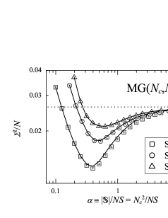
Figure 1: The mean variance $\Sigma^{2}$ versus the control parameter $\alpha\equiv|{\mathbb{S}}|/NS=N_{c}^{2}/NS$ in MG($N_{c}$,$N_{c}^{2}$) with different number of strategies $S$ where $N_{c}=37$ and $M=2$. The solid lines are the predictions of the crowd-anticrowd theory whereas the dashed line indicates the coin-tossed value.

Fig. 1 shows the mean variance of attendance as a function of the control parameter $\alpha$ in the MG($N_{c}$,$N_{c}^{2}$) for a typical $N_{c}$. For the MG($N_{c}$,$N_{c}^{2}$), the mean variance of attendance, $\Sigma^{2}$, exhibits similar behavior as a function of the control parameter $\alpha$ to that in the MG no matter how many strategies $S$ players have. In particular, whenever $N_{c}^{2}/NS\approx 1$, the mean variance $\Sigma^{2}$ is smaller than the so-called coin-tossed value. (Coin-tossed value is the mean variance resulting from players making random choices.) Thus, global cooperation amongst the players is observed in this parameter range. Moreover, Fig. 1 shows that the mean variance predicted by the crowd-anticrowd theory agrees with our numerical finding.

Further results along this line, including the mean variance of attendance as a function of the control parameter in MG($N_{c}$,$N_{c}^{2}$) with different strategy space ${\mathbb{S}}$, will be reported elsewhere. These results all agree with the crowd-anticrowd theory Min14 . Therefore, we conclude that we have successfully build up the MG($N_{c}$,$N_{c}^{2}$) model whenever $N_{c}$ is a prime power.

Indeed, the MG($N_{c}$,$N_{c}^{2}$) model can be readily extended to MG($N_{c}$,$N_{c}^{k}$) with $N_{c}$ is equal to a prime power for $3\leq k\leq M+1$. We found that the mean variance also agrees with the MG and the crowd-anticrowd theory in the MG($N_{c}$,$N_{c}^{k}$) Min14 . Thus we can always alter the complexity of each strategy in MG with fixed $N$, $S$ and $M$ while the cooperative behavior still persist. As a result, we can always keep (almost) optimal cooperation amongst the players in almost the entire parameter space.

However, is it possible to construct a MG with $N_{c}$ alternatives whose strategy space size is smaller than $N_{c}^{2}$ that exhibits global cooperation? We give the answer by constructing the MG($N_{c}$,$\eta N_{c}$) model where $\eta$ is an integer less than $N_{c}$.

The basic setting of MG($N_{c}$,$\eta N_{c}$) is the same as that of MG($N_{c}$,$N_{c}^{2}$) except that the strategies are drawn from a different strategy space. More precisely, strategies of MG($N_{c}$,$\eta N_{c}$) are picked from the set ${\mathbb{S}}_{K}=\{\lambda_{a}\vec{v}_{a}+\lambda_{u}\vec{v}_{u}:\lambda_{a}\in GF(N_{c}),\lambda_{u}\in K\subset GF(N_{c})\}$ where $K$ contains $\eta$ elements. Moreover, $\vec{v}_{a}$ and $\vec{v}_{u}$ satisfy the two technical conditions in Eqs. (1) and (2). Clearly, the strategy space size of ${\mathbb{S}}_{K}$ equals $\eta N_{c}$.

Figure 2: The mean variance $\Sigma^{2}$ (square) versus the control parameter $\alpha\equiv|{\mathbb{S}}_{K}|/NS=\eta N_{c}/NS$ in MG($N_{c}$,$\eta N_{c}$) with different $\eta$ where $S=2$ and $M=2$. The variance of the attendance of a choice (cross) is also shown in the figure. The solid line indicates the mean variance predicted by the crowd-anticrowd theory whereas the dashed line indicates the coin-tossed value.

As shown in Fig. 2, the mean variance of attendance $\Sigma^{2}$ in MG($N_{c}$,$\eta N_{c}$) shows similar behavior as a function of the control parameter $\alpha$ to that in the MG only for small $\alpha$. When $\alpha$ increases, the mean variance $\Sigma^{2}$ in MG($N_{c}$,$\eta N_{c}$) becomes smaller than that in MG. Nevertheless, the numerical mean variance in MG($N_{c}$,$\eta N_{c}$) does not agree with the prediction of the crowd-anticrowd theory except for small $\alpha$. The inconsistency is more pronounced when $\alpha$ increases.

To account for this discrepancy, we notice that as $\eta\rightarrow 1^{+}$ while keeping all other parameters fixed, fewer and fewer (or even none) of the strategies in the strategy space of MG($N_{c}$,$\eta N_{c}$) makes the same choice for the same combination of the output of the last $M$ steps. Therefore, some of the choices can never be chosen for MG($N_{c}$,$\eta N_{c}$) with small $\eta$ when the number of strageties picked by the players are much smaller than the strategy space size $\eta N_{c}$. In this circumstances, the attendances of most alternatives are either one or zero. Consequently, the mean variance $\Sigma^{2}$ in MG($N_{c}$,$\eta N_{c}$) with small $\eta$ is much less than $N$. In fact, the variance of a choice may even vanished for large $\alpha$. Such phenomenon will be more pronounced in MG($N_{c}$,$\eta N_{c}$) with small $\eta$. Thus, the mean variance in the MG($N_{c}$,$\eta N_{c}$) for $\eta\ll N_{c}$ exhibits a radically different behavior from the MG. From the above observation, we know that there is no effective crowd-anticrowd interaction whenever $\eta\ll N_{c}$. And in this case, the dynamics in the MG($N_{c}$,$\eta N_{c}$) is no longer dominated by the interactions of the anti-correlated strategies. Consequently, the crowd-anticrowd theory does not correctly predict the mean variance in MG($N_{c}$,$\eta N_{c}$). Nonetheless, we still find that in MG($N_{c}$,$\eta N_{c}$), $\Sigma^{2}$ attains a minimum (and hence the average number of winning players is maximized) whenever the control parameter $\alpha\equiv|{\mathbb{S}}_{K}|/NS=\eta N_{c}/NS\approx 1$ for every prime power $N_{c}$ and $1<\eta<N_{c}$.

Now, we are ready to answer the two questions posted in the abstract. First, in order to obtain the best overall global wealth, players should switch to the MG($N_{c}$,$\zeta N_{c}$) game provided that $N_{c}<NS\leq N_{c}^{M+1}$. More specifically, for fixed $N_{c}$, $N$, $S$ and $M$, players simply have to agree on an integer $\zeta\approx NS/N_{c}$ and the corresponding strategy space in order to ensure the best performance of the MG. Second, whenever $\zeta\geq N_{c}$, the mean variance of attendance $\Sigma^{2}$ agrees well with our extension of the crowd-anticrowd theory. Thus, we conclude that in MG($N_{c}$,$\zeta N_{c}$) with $N_{c}\leq\zeta\leq N_{c}^{M}$, the origin of global cooperation is the self-organization of player’s tendency to choose anti-correlated strategies in making their decision. The “cancellation” of the actions in these mutually anti-correlated strategy ensemble leads to a small $\Sigma^{2}$.

Finally, we remark that results on the order parameter of MG($N_{c}$,$\zeta N_{c}$) will be reported elsewhere Min14 . Readers should note that in case $N_{c}$ is not a prime power, the presence of zero divisors in the ring ${\mathbb{Z}}_{N_{c}}$ invalidates the conclusion in Eq. (9). So, it is instructive to find a reasonable extension of MG($N_{c}$,$N_{c}^{2}$) in this case.

Useful discussions with K. H. Ho, P. M. Hui and Kuen Lee is gratefully acknowledged. This work is support by the RGC grant of the Hong Kong SAR government under the contract number HKU 7098/00P. H.F.C. is also supported in part by the University of Hong Kong Outstanding Young Researcher Award.

References

- (1) D. Challet and Y. C. Zhang, Physica A 246, 407 (1997).
- (2) Y. C. Zhang, Europhys. News 29, 51 (1998).
- (3) W. B. Arthur, Amer. Econ. Assoc. Papers and Proc. 84, 406 (1994).
- (4) D. Challet and Y. C. Zhang, Physica A 256, 514 (1998).
- (5) R. Savit, R. Manuca and R. Riolo, Phys. Rev. Lett. 82, 2203 (1999).
- (6) N. F. Johnson, S. Jarvis, R. Jonson, P. Cheung, Y. R. Kwong and P. M. Hui, Physica A 258, 230 (1998).
- (7) D. Challet and M. Marsili, Phys. Rev. E 60, R6271 (1999).
- (8) D. Challet, M. Marsili and R. Zecchina, Phys. Rev. Lett. 84, 1824 (2000).
- (9) M. Hart, P. Jefferies, N. F. Johnson and P. M. Hui, Physica A 298, 537 (2001).
- (10) M. Hart, P. Jefferies, N. F. Johnson and P. M. Hui, Eur. Phys. J. B 20, 547 (2001).
- (11) F. K. Chow and H. F. Chau, cond-mat/0109166.
- (12) A. Cavagna, Phys. Rev. E 59, R3783 (1999).
- (13) D. Challet and M. Marsili, Phys. Rev. E 62, R1862 (2000).
- (14) H. F. Chau and F. K. Chow, in preparation.