Nonparametric modeling and spatiotemporal dynamical systems

Abstract

In this article, it is described how to use statistical data analysis to obtain models directly from data. The focus is put on finding nonlinearities within a generalized additive model. These models are found by the means of backfitting algorithms or more general versions, like the alternating conditional expectation value method. The method is illustrated by numerically generated data. As an application the example of vortex ripple dynamics, a highly complex fluid-granular system is treated.

1 Introduction

One of the major goals of spatiotemporal data analysis consists in inferring a model from a given spatiotemporal data set. Conventional ways of modeling are purely theoretical arguing and a posteriori evaluation of possible models with suitable measures. In this article, statistical methods and applications to infer generalized additive models from data are presented. The attention is put on spatio-temporal systems, but there are certainly more possibilities of using the ideas in physics and engineering. Generalized additive models have been introduced to statistical analysis in the 1980’s [1, 2]. The development of solving algorithms and mathematical proofs has been developed contemporarily (see [2] and references therein).

During the last two decades, natural sciences profited a lot by the increasing computer power of modern machines. In nonlinear and statistical sciences, old techniques could be exploited to their full extent and new methods have been developed. The identification of nonlinearities is one of the important topics in data analysis of. e.g., chaotic or pattern forming systems [3, 4]. This in turn is feasible by statistical tools.

Careful application of algorithms and thorough interpretation of results leads to a direct way to obtain models from data. Hereafter, the basic ideas of the techniques to solve for a generalized additive model are explained and an application to spatio-temporal data is given. The intention is not to give a full overview of statistical methods, nor to report an experiment in detail. Rather, it is shown how a consistent procedure to infer models from data can be used as a feedback to theory which in turn can motivate experimental designs to yield new data and so on.

The paper is structured as follows: In Sec. 2 the algorithmic solutions for generalized additive models are pointed out. This is done by the example of ACE, the Alternating Conditional Expectation value algorithm, which uses the backfitting technique. This presentation is given some room; even though nothing new for statisticians, technical points need some explanation to be understood. Sec. 3 provides more information to be used in the context of spatio-temporal data analysis. In Sec. 4 problems arising from preprocessing of data are discussed along with the pattern formation example of vortex ripple dynamics. The paper concludes with a short discussion in Sec. 5.

2 Generalized additive models and backfitting

The standard tool of data analysis for physicists and engineers is the multivariate linear regression, where one fits the model

$$U_{0}=C+\sum_{i=1}^{M}\alpha_{i}U_{i}+\epsilon\;$$ (1)

to experimental data. The symbols $\epsilon$ and $U_{i}$ (upper case letters), $i=0,\dots,M$ denote a random process with given distribution, $C$ is a constant and the $\alpha_{i}$ are model parameters. One measures a realization $u_{i}$ (lower case letters), $i=0,\dots,M$ of the random process and finds estimates $\hat{\alpha_{i}}$ for the parameters, e.g., by least squares fitting [5]. Throughout the text, estimations are denoted by a hat, only where ambiguity exists, otherwise additional symbols are omitted.

There are many ways of generalization. One often used way is the generalized linear regression model,

$$U_{0}=C+\sum_{i=1}^{M}\alpha_{i}f_{i}(U_{i})+\epsilon\;.$$ (2)

In this model, the data analyst chooses beforehand the functions $f_{i}$ due to some prior knowledge about the system or simply by guessing. Then, a linear regression procedure yields estimates for the parameters $\alpha_{i}$. So, the model is expressed in parametric form by the estimates $\hat{\alpha_{i}}$. For details about linear regression, see, e.g., [5, 6].

If no obvious choice for a function is at hand, it is desirable to fit the nonparametric model

$$U_{0}=C+\sum_{i=1}^{M}f_{i}(U_{i})+\epsilon\;.$$ (3)

Given some data, estimates $\hat{f_{i}}$ must result. With this kind of modeling no prior knowledge about functional dependences is needed as input; one can find very general functional forms. A disadvantage is the absence of even more general terms, like $f_{i}(U_{i},\,U_{j})$, $j\neq i$. The reason for this lack is a practical one: as will become clear below, any implementation finding functions of $d$ variables has to compete with the curse of dimensionality. For the generalized additive model (3), estimates for the functions $f_{i}$ are found by the backfitting algorithm [1, 2, 7]. This is an iterative procedure, working by the following rules:

1. Initialization: $C=E(U_{0})$, $f_{i}=f_{i}^{0}$, $i=1,...,M$.

2. Iteration: for $i=1,...,M$ calculate

   $$f_{i}=E\left(U_{0}-C-\sum_{k\neq i}f_{k}(U_{k})|U_{k}\right)$$

   until convergence,

where $E()$ denotes the expectation value and the $f_{i}^{0}$ are some appropriate initial settings. In applications, one has to obtain the functions from data as realizations of the generating process. Then, this operator has to be replaced by its estimator. In each iteration step we estimate the functions by $\hat{f_{i}}(U_{i})=S_{i}(\cdot|U_{i})$, a smoothing operator which returns a function dependent on $U_{i}$.

The discussion of properties and choice of the smoother is a subtle issue and lies far beyond the scope of this paper, a detailed discussion is given in [8]. The examples presented in this article have been obtained using the simple running mean smoother (moving average). This is not the best choice for many problems, e.g., points at the boundaries have to be considered with care or must be cut - throughout this article, there have been enough data to afford for the luxury to cut the boundaries, in spatio-temporal systems there are often many thousand of data points. Smoothing splines are good smoothers in many situations due to their differentiability properties [2, 8]. In any case, a careful check should be undertaken for a concrete set of data.

The iteration works by adjusting only for one function, subtracting all the others from the estimation of $U_{0}$, i.e. one smoothes the partial residual $(U_{0}-\sum_{k}f_{k})$ against $U_{i}$. In spatiotemporal data analysis, on is faced with the task of finding equations of motion from data. These can be coupled map lattices, a set of ordinary coupled differential equations, partial differential equations or even more complicated models. In many of these formulae, the lhs. is linear (e.g. a time derivative) and Eq. (3) constitutes an appropriate additive, nonlinear model. If the measured data are nonlinear transforms through a measuring function, it can be desirable to model a nonlinear lhs, too:

$$f_{0}(U_{0})=C+\sum_{i=1}^{M}f_{i}(U_{i})+\epsilon\;.$$ (4)

The constant can be absorbed w.l.o.g. into the functions $f_{i}$. Now, the model is more symmetrical and indeed, in physics, often situations without a clear predictor (lhs) - response (rhs) structure are found. A typical example is pattern formation where one is interested in the nonlinear interaction of stationary states. A priori it is not clear which variables constitute the state space nor is it always possible to measure them. Data analysis provides then an estimation of the model as a nonlinear, possibly noninvertible, transformation of the measured data. As an example, take the relation $U_{0}=G(U_{1}+U_{2})$ with $G$ some nonlinear invertible function. The inverted equation $G^{-1}(U_{0})=U_{1}+U_{2}$ cannot be found with (3), but with the model (5). An example for this case is given below.

An algorithm to solve (4) is ACE, (the Alternating Conditional Expectation value algorithm) [9], it works by minimizing the squared error

$$E\left[f_{0}(U_{0})-\sum_{i=1}^{M}f_{i}(U_{i})\right]^{2}\;.$$ (5)

The method shall be explained stepping from the one-dimensional estimation over two dimensional to the M-dimensional problem.

1) $U_{0}=f_{1}(U_{1})+\epsilon$.

For this simple model, one obtains from Eq. (5)

$$E\left[U_{0}-f_{1}(U_{1})\right]^{2}=min,$$ (6)

where minimization is achieved by variation of $f_{1}$ in the space of measurable functions [9]. After some elementary steps one finds the solution [10]

$$f_{1}(U_{1})=E(U_{0}|U_{1})\;.$$ (7)

For applications, again a smoother is used as estimator of the expectation value operator. The result of the smoothing on a set of numerically produced data is shown for the example $U_{0}=U_{1}^{2}$ in Fig. 1. The data has been generated by first drawing 10 000 equally distributed random numbers for $u_{1}$ in the interval $(-3,3)$. These numbers have been squared to yield the values for $u_{0}$, after this Gaussian noise $N(0,0.1^{2})$ has been added. The bandwidth of the running mean smoother has been set here and below to 200 points. In Fig. 1, the scatterplot of the points $(u_{1},u_{0})$ is shown (grey) together with the estimate for the function $f_{1}$, found by Eq. (7) (black, thick line). As indication for the estimation error the pointwise standard deviation has been calculated from the estimated function and the residuals (upper and lower black lines).

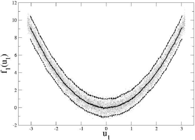
Figure 1: One step transformation in the case $f_{0}=U_{0}$, $f_{1}(U_{1})=U_{1}^{2}$. The scatterplot of points $(u_{0},u_{1})$ is shown by grey dots (not labelled). Applying the running mean smoother yields an estimation for the function $f_{1}$ (middle, thick black line), above and below is plotted twice the pointwise standard deviation (upper and lower black lines).

2) $\;\;f_{0}(U_{0})=f_{1}(U_{1})+\epsilon\;$.

In this case, the solution is found iteratively:

1. Initialization: $f_{0}(U_{0})=\left[U_{0}-E(U_{0})\right]/\sqrt{var(U_{0})}$.

2. Computation of $f_{1}(U_{1})=E[f_{0}(U_{0})|U_{1}]$

3. Computation of $\tilde{f_{0}}(U_{0})=E[f_{1}(U_{1})|U_{0}]$

4. Normalization: $f_{0}(U_{0})=\tilde{f_{0}}(U_{0})/\sqrt{var(\tilde{f_{0}}(U_{0}))}$.

5. Iteration of 2)-4) until convergence.

A smoother with nonzero bandwidth is contracting and thus the trivial solution is excluded by normalization (point 4) with the variance $var(\tilde{f_{0}}(U_{0}))$.

In order to show how ACE handles non-invertible relations, data ($A\cos\theta$, $A\sin\theta$) have been generated, with $\theta=\varphi+\epsilon_{\varphi}$ and $\varphi$ an equally distributed random number in $[0,2\pi)$ and $A=1+\epsilon_{A}$. The noise $\epsilon_{\varphi}\,,\epsilon_{A}$ is Gaussian distributed, with $N(0,0.05^{2})$. This corresponds to the noisy measurement of an amplitude and a phase with a nonlinear, noninvertible measurement transformation.

Without noise, one has $U_{0}=\cos(\varphi)$, $U_{1}=\sin(\varphi)$ and thus $U_{0}^{2}=1-U_{1}^{2}$. With noise, the relation reads to first order $U_{0}^{2}-2\epsilon_{A}\,U_{0}=1-U_{1}^{2}+2\epsilon_{A}\,U_{1}$. This means that multiplicative noise enters in predictor and response, touching the errors in variables problem which is relevant for many applications. The strong, multiplicative transformation of the noise is mirrored directly in the results.

In Fig. 2 a) the data are displayed in a scatterplot, in Fig. 2 b) and c), the resulting functions are shown on top of the respective residuals together with twice the pointwise standard deviation as an error indicator. Due to the nonlinear noise transformation the functions are distorted. The pointwise standard deviation is less significant as error indicator due to the very asymmetric local distribution of values, to be seen in the upper and lower curves of Fig. 2 b) and c). In this case asymmetric measures should be calculated. The above example underlines a conceptual problem when one is faced with errors in the measurement variables. The general treatment of this problem is not simple, for more details see [11, 12] and references therein.

Even though the precise estimation of the functional dependence is not possible in the above case, one finds an approximation which would not be so bad for many experiments. Please note that linear tools would not be able to find this relation easily, rather one should undergo a trial-and-error procedure until a guess for the right form of the functions is found. Some problems with a non-Gaussian distribution, however, remain in linear regression, too.

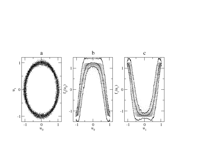
Figure 2: Example for $U_{0}=A\,\sin\theta$, $U_{1}=A\,\cos\theta$, where $A$ and $\theta$ include measurement noise (a). The expected functional relation is noninvertible: $U_{0}^{2}+U_{1}^{2}=1$, noise on $A,\theta$ is transformed nonlinearly. The grey dots in (b), (c) show this effect in the residuals. This in turn influences the result in that it induces bending at the ends and in the center part of the results of ACE, where the transformation has its biggest effect $f_{0}$ and $f_{1}$ (see the middle line in (b), (c)). The symmetric pointwise standard deviation is not a good indicator for the asymmetry (upper and lower lines in (b), (c)), according asymmetric measures should be calculated. Functions are shifted to zero mean.

3)$\;\;f_{0}(U_{0})=\sum_{i=1}^{M}f_{i}(U_{i})+\epsilon\;$

This equation defines a (noisy) hypersurface in $M$-dimensional space (in two dimensions, one finds a line). The functions $f_{i}$, fall on a hyperplane: the algorithm performs a transformation of the points $\{U_{1},\dots,U_{M}\}$ to the points $\{f_{1},\dots,f_{M}\}$ such that the best plane in the mean squared sense is found.

The modification in the algorithm has to be done in the steps 2. and 3. above. They are replaced by

1. Computation of $f_{i}(U_{i})=E[f_{0}(U_{0})-\sum_{k\neq i}f_{k}(U_{k})|U_{i}]$ by backfitting.

2. Computation of $\tilde{f_{0}}(U_{0})=E[\sum_{i}f_{i}(U_{i})\,|\,U_{0}]$

This shows that the ACE algorithm is based on backfitting. To demonstrate a higher-dimensional example, the relation $U_{0}=\exp(U_{1}+U_{2}^{2})$ has been chosen. The variables have been generated using equally distributed values for $U_{1}\,,U_{2}$ in the interval $(-2,2)$. From the resulting numbers, $u_{0}$ has been calculated, thus the smallest possible value of $u_{0}$ is $\exp(-2)\simeq 0.14$, the largest is $\exp(6)\simeq 400$. After this procedure (in contrast to the previous example), Gaussian, $N(0,0.2^{2})$, noise has been added to $u_{i}$, $i=0,1,2$. This avoids the problems with transformation of measurement noise, discussed above. But at this place, another interesting question for the modeler is raised instead: what happens if one tries to include some additionally measured variable in the model?

As an example, one can imagine a measurement of four variables, where it is not clear a priori which variables are needed in a minimal model. As a first guess, a generalized additive model $f_{0}(U_{0})=f_{1}(U_{1})+f_{2}(U_{2})+f_{2}(U_{3})$ will be tested. This situation shall be now related to the data generated above: an additional, equally distributed variable in the interval $(0,100)$, uncorrelated to $U_{0},\,U_{1},\,U_{2}$, is generated and fed as fourth variable into ACE.

The three-variable additive model is $f_{0}(U_{0})=f_{1}(U_{1})+f_{2}(U_{2})$ and one expects ACE to find the estimates $\hat{f_{0}}(U_{0})=\ln(U_{0})\,,\hat{f_{1}}(U_{1})=U_{1}\,,\hat{f_{2}}(U_{2})=U_{2}^{2}$ due to the additive structure. For the four dimensional model, one expects an unchanged result for $\hat{f_{0}},\,\hat{f_{1}},\,\hat{f_{2}}$ plus a zero function $\hat{f_{3}}(U_{3})=0$ in the additional variable.

In Fig. 3, the 3D scatterplot of the generated relevant data is shown by the points $(\ln(U_{0}),U_{1},U_{2})$, the $U_{0}$-axis is logarithmic. A two dimensional representation is not able to display the full relation, if one plots, e.g., $U_{0}$ vs. $U_{1}$ (Fig. 4), no functional dependence is cognizable. The transformations $(\hat{f_{0}},\hat{f_{1}},\hat{f_{2}},\hat{f_{3}})$ found by ACE are shown in Fig. 5 as functions of their arguments. The function $f_{0}$ is found to be logarithmic, $f_{0}=0.5\,\ln(u_{0})+c$, $f_{1}$ is linear with a slope of $0.5$, and $f_{2}=au_{2}^{2}+c$ is quadratic also with a factor $a=0.5$. The factor $0.5$ reflects possible ambiguities in the result, as well as the addition of the constant, see Sec. 3.2.

After multiplying the results by $2$ and adding a constant to $f_{0}$ and $f_{2}$ one can speak of a good coincidence of expected and found result. The additional variable $u_{3}$ has no dependence on the others and yields $f_{3}=O(10^{-2})\simeq 0$. Thus, the method is able to identify uncorrelated terms. A comparison of runs with and without the additional third term on the rhs showed that the functions are virtually unchanged, confirming the stability of the algorithm. Despite the seemingly convincing result it must be noted that results can be misleading if there exist correlations between an additional term and “true” variables. If the task is to find a minimal model, one has to consider this effect. The connection of correlation with ACE is discussed in Sec.3.3.

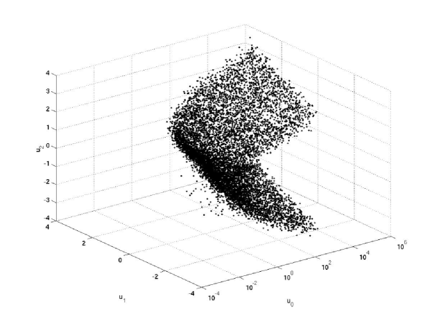
Figure 3: Three dimensional plot of the data from $U_{0}=\exp(U_{1}+U_{2}^{2})+\epsilon$.

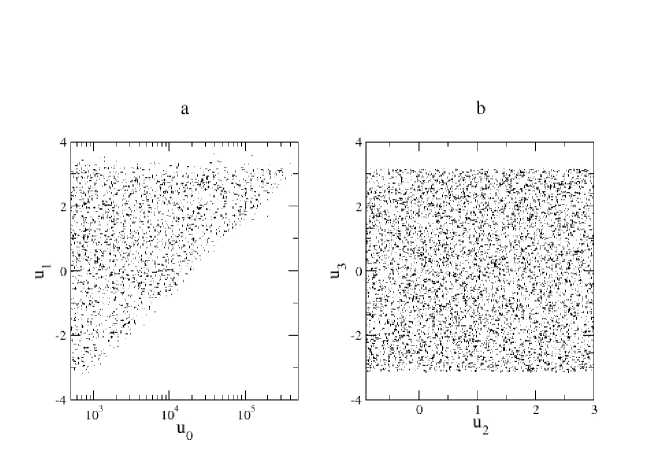
Figure 4: Two dimensional scatter plots of a part of the data as projection on the plane. The examples $u_{0}\,,u_{1}$ and $u_{2}\,,u_{3}$ are shown. even “guessing” a logarithmic relation for $u_{0}$, no clear relation can be read on the left, on the right, the data are completely random according to the zero correlation of $u_{3}$ with the rest.

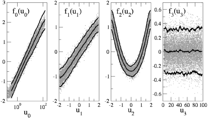
Figure 5: Transformations for the given data with twice the pointwise standard errors (black lines) on top of the residuals (grey). The logarithm $f_{0}(u_{0})$ is found over three decades to hit numerical restrictions at the smallest points. The linear and square functions $f_{1}$ and $f_{2}$ are found very well. The variable $u_{3}$ is found to be “unimportant” with $f_{3}(u_{3})=0$.

3 Some further topics

3.1 Smoothers and the bias-variance dilemma

As mentioned above, the choice of the smoother can be delicate. Typically, to each smoother belongs a smoothing parameter which characterizes its bandwidth (window width). For the running mean smoother, one obtains for problem (7)

$$\hat{f}_{1}(U_{1,l})=1/N_{l}\sum_{j\in B(U_{0,l})}U_{0,j}\;,$$ (8)

where the hat denotes estimation and $B(U_{0,l})$ is a neighborhood of the point $U_{0,l}$. Increasing bandwidth enlarges the neighborhood and thus the number $N_{l}$ of data points in $B$. The respective expectation and variance are

$$E(\hat{f}_{1}(U_{1,l})) = 1/N_{l}\sum_{j\in B(U_{0,l})}f(U_{0,j})\;,$$ (9)

$$var(\hat{f}_{1}(U_{1,l})) = \sigma^{2}/N_{l}\;,$$ (10)

where $\sigma_{l}=\sigma$ is assumed for simplicity. Thus, the variance shrinks with increasing bandwidth; the bias, however, increases because more terms different from $f(U_{0,l})$ are involved. If one wants to find the optimum choice of the bandwidth in order to have neither large bias nor large variance, one uses measures like the mean-squared error or the average predictive squared error; these are evaluated using cross-validation and yield a criterion for the bandwidth to be chosen. For more information it is referred to the literature [2, 10].

The iteration procedure should run until convergence. In fact, convergence is not guaranteed for all classes of smoothers, asymptotic properties and convergence is discussed in a rigorous way in [9, 8, 13]. Intuitively, it is clear that the iteration should stop when the errors on the functions fall below the noise $\epsilon$ in the model (4). Then it is a question how to find properly the respective errors. There are different ways to estimate the error consistently, depending on the smoother and the error models used. Locally, one can choose twice the pointwise standard error as a characterization, global confidence criteria are harder to derive [2, 11], an elegant and modern approach is given by the Bayesian formulation of the backfitting algorithm [14]. In the case of errors in variables, care has to be taken to calculate the error correctly, a Bayesian approach is appealing in that case. In the examples, the most naive criterion, i.e., twice the pointwise standard error has been used.

3.2 Peculiarities of ACE

The ACE algorithm can be related to other algorithms, namely canonical variates and alternating least squares methods. Special properties of all three methods are discussed in [15], peculiarities of ACE are discussed in [2, 9], here a few items shall be given without a claim for completeness.
i) ACE is symmetric in the predictor and the response, which is quite unusual for a regression tool, but suits well several setups in physical applications.
ii) Transformations of the variables are not reproduced by ACE. Take, e.g., the case $U_{0}=f_{1}(U_{1})+\epsilon$. If one applies a transformation to each of the sides, ACE does not necessarily find $f_{1}$ again. This reflects parts of the nature of the inverse problem, which is in general not uniquely solvable. Especially, adding a constant to either of the sides in the model is ambiguous in ACE.
iii) Different distributions in the model constituents can “distort” the resulting functions. E.g., it may happen that one term in a model with two variables is Gaussian distributed and another one is equally distributed in some interval. Then, the Gaussian variable is bent at the ends (cf. Fig. 5).

3.3 Maximal Correlation

The ACE algorithm can be regarded as a regression tool, but there exists another possible interpretation. Instead of solving the least squares error minimization problem

$$E[f_{0}(U_{0})-\sum_{i=1}^{M}f_{i}(U_{i})]^{2}=min$$ (11)

one can reformulate the above to

$$\Psi=corr\left(f_{0}(U_{0}),\,\sum_{i=1}^{M}f_{i}(U_{i})\right)=max\;,$$ (12)

where $corr$ denotes the correlation function. This reflects the principle of the maximal correlation [16, 17, 18, 19]. The functions that fulfill Eq. (12) are called optimal (in the sense of correlation) transformations, found by the ACE procedure. To have a global measure for the importance of a single term $f_{i}(U_{i})$ , there are several possibilities, e.g., one can choose the overall variance, $var(f_{i})$, but this does not reflect correlation with other terms and a noise term with large variance would be judged to be important. Here, the author suggests to use Eq. (12) in a symmetric way,

$$\Psi_{i}=\left|\frac{E(f_{i}\cdot\sum_{j\neq i}f_{j})}{\sqrt{E(f_{i}^{2})\cdot E(\sum_{j\neq i}f_{j})^{2}}}\right|\;,$$ (13)

to characterize the importance of a single term. The use of this measure is demonstrated for the data from the example used for Fig. 5. The values $\Psi_{0}=0.9779$, $\Psi_{1}=0.9272$, $\Psi_{2}=0.9690$ and $\Psi_{3}=0.0426$ are found, confirming again the unimportance of the additional uncorrelated variable, this time by the global measure $\Psi_{3}$.

If however, the additional variable is correlated, e.g., by passively following another variable, a high correlation will follow, yielding a model with more components. In the case of spatiotemporal modeling one has to be specially careful, because one is interested in minimal (in the number of terms) models, but dynamical dependencies can result easily in correlations, like in the case of slaved variables.

3.4 Generalizations

One can generalize the procedure to include more complex, non-additive couplings, e.g. in the three dimensional case, one considers the model

$$U_{0}=F(U_{1},U_{2})+\epsilon\;,$$ (14)

with $F$ some function, describing a two dimensional surface in a three dimensional space spanned by $U_{0},\,U_{1},\,U_{2}$. Like for Eq. (7), one finds

$$F(U_{1},U_{2})=E(U_{0}|U_{1},U_{2})\;.$$ (15)

Going to higher dimensions requires in general more data due to the curse of dimensionality, additionally one has to decide again which estimator to use for correct results.

As an example, the relation $U_{0}=U_{1}\cdot U_{2}$ (Fig. 6a) is used. Ten thousand equally distributed data points in the range $(-1,1)$ for $U_{1},\,U_{2}$ have been generated, from these $U_{0}$ is obtained by multiplication. Gaussian, $N(0,0.1^{2}$, noise has been added afterwards to each of the three variables as noise realizations. The estimated function coincides well with the expectation (Fig. 6b). Note that in this case ACE yields as a result $\log U_{0}=\log U_{1}+\log U_{2}$ because of the additive structure of the model (5)

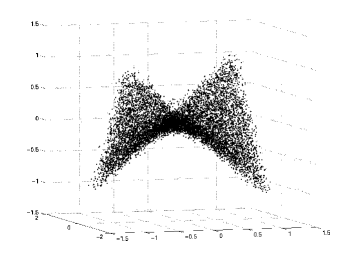
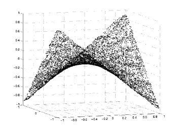
Figure 6: Left: noisy data for the surface $U_{0}=U_{1}\cdot U_{2}$, $\sigma=0.05$ for all $U_{i}$. Right: Optimal two dimensional transformation. The result is very good, the CEV smoother is able to accurately find the hyperbolic profile.

For this model, many applications with quasi-two-dimensional setting can be found, e.g., in geological and hydrodynamical systems (e.g. the two dimensional Euler equations).

4 Application to spatiotemporal data

Typical spatiotemporal models of interest for a physicist are coupled map (CML) systems , coupled ordinary differential equations (ODE’s) or partial differential equations (PDE’s). In all these models, derivatives or finite differences are involved. Here, the measured quantity shall consist of a space-time record, given by a movie, i.e. a series of consecutive pictures. From the time series in one point one builds finite differences in time, from the pictures one calculates differences in space. This procedure is numerically not trivial: addition (or subtraction, respectively) is numerically bad conditioned and can yield extinction of digits, measurement noise is then shifted to the first digits. Basically, one must use the apparatus known from numerical integration [5, 20, 21] to use correct sampling in space and time. In the case of a periodic setup, accuracy loss can be limited by using spectral methods [5, 22].

As an example, let us take the Complex Ginzburg-Landau Equation. It describes a well pattern formating system above onset [23]:

$$\partial_{t}A=(1+ic_{1})\Delta A+(1-ic_{3})f_{1}(|A|^{2})A\;.$$ (16)

The function $f_{1}$ is a complex nonlinear function. The task of data analysis -supposed that $A$ can be measured- is to determine the nonlinearity $f_{1}$. To apply the ideas of backfitting we put $U_{0}(x,t)=\partial_{t}A/A$, $U_{1}(x,t)=\Delta A/A$, $U_{2}(x,t)=|A|^{2}$. Real and imaginary part must be treated separately. Using the iteration procedure, one finally obtains estimates for the parameters $c_{1}$, $c_{3}$ and the full function $f_{1}$. In a slightly more complicated setup, this has been performed in [24]. In fact, for this example the numerically critical step is rather the correct evaluation of derivatives than the application of backfitting.

If one wants to find a model, but there are no physical arguments which derivatives should occur or it is even unclear if the measured quantities are state variables or have undergone some measurement transformations, one can still try to find a generalized additive model. In that case, it can be worth to fit a discrete model (CML), that represents the system dynamics, avoiding a good part of the trouble with finite differences (one can choose mapping units big enough to avoid numerical problems).

A recently presented experiment considers underwater vortex ripples [25, 26]. The ripple formation is driven by a periodical motion of water over a sand bed with given amplitude and frequency. A picture of the ripples -viewed from the side- is given in Fig. 7 a), the resulting space time plot is shown in Fig. 7 b). In this paper, experimental details are not given, for those it is referred to the literature [26, 27]. But the treatment of the data and subsequent results are presented to demonstrate application of the nonparametric regression.

a)

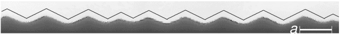
b)

Figure 7: a) Ripple profile as observed in the experiment. The driving amplitude $a$ is marked. With the bottom at rest, water is oscillating forth and back over the crests. Triangles (top, black line) are fitted to raw picture (lower, dark profile) to determine the crests. b) The experimental evolution of the position of the ripple crests starting from ripples with a small length yields the shown space time plot.

The model is formed by coarse graining of space and time. In time, one uses a mapping from period to period, in space, ripples are characterized by their length $\lambda$. The interaction between ripples is modeled by a nonlinear interaction function which must be concave by stability analysis. The model is obtained for ripples close to the final length; without discussing further the physical mechanisms, it reads:

$$\lambda_{i}(T+1)-\lambda_{i}(T)=-f(\lambda_{i-1(T)})+f(\lambda_{i}(T))-f(\lambda_{i+1}(T))+\epsilon\;.$$ (17)

The subscript $i$ denotes the space index.

The process of data analysis involved the following steps:
i) calculating the ripple length, this has been done by fitting triangles to the raw profiles and calculating the distances from crest to crest (cf. Fig. 7. The accuracy amounted to two digits.
ii) Calculation of the rhs of Eq. (17), this has been done by first calculating the difference, the result has been very noisy due to the numerical extinction of digits. To compensate for this effect, the differences have been smoothed and small numbers have been discarded. Please note that no “unsuitable” points have been excluded (a common, but often wrong technique for outliers), rather it is a numerical requirement. In any case, the model has been developed from considerations of long ripples not too far from the final length and thus very small ripples are not expected to follow the model dynamics.
iii) To apply a backfitting algorithm, one has to identify the variables $U_{i}$ as they have been denoted in the previous sections. We put formally $\Delta_{t}~{}\lambda~{}=~{}\lambda_{i}(T+1)-\lambda_{i}(T)=U_{0}$, $\lambda_{i-1}(T)=U_{1}$, $\lambda_{i}(T)=U_{2}$, and $\lambda_{i+1}(T)=U_{3}$. The lhs shall be linear, so the model (3) has been used. For this example, the functions are denoted by $f_{1}=f_{l}$, $f_{2}=f_{c}$, $f_{3}=f_{r}$, for the left, center and right one, respectively. In the present context this allows easier interpretation in terms of the spatial structure. The data under consideration have been obtained by nine experimental runs, each between 1000 and 6000 data points.

The experimental runs have been stationary as far as experimental technique is concerned. Each data point $(\Delta_{t}\lambda_{i}(T),\lambda_{i-1}(T),\lambda_{i}(T),\lambda_{i+1}(T))$ can be considered as an independent realization of the underlying process. Thus, the data from all nine measurements have been analyzed together. The result is shown in Fig. 8. For each function, the importance criterion is calculated with $\Psi_{0}=0.732$, $\Psi_{1}=0.560$, $\Psi_{2}=0.8604$ and $\Psi_{3}=0.6376$. From these numbers one obtains basically two informations: 1) There is a large part of variance which cannot be modeled. This can have two reasons, the first is measurement noise, which has been reduced as much as possible, the second is that parts of the dynamical equations (higher order interactions or similar) are not included in the model. A priori it is not easy (or even impossible) to distinguish which is the reason, again the error in variables problem has to be treated with care. 2) The growth of a ripple depends mainly on the length of this ripple, but the neighbors cannot be neglected. This is seen by the lower correlations for the neighboring functions.

As a basic test, the result functions must show the expected concave shape. This is perfectly true in the range the model should hold. There are, however differences between the neighbor functions $f_{l}$, $f_{r}$ and the center one, $f_{c}$. Mainly one notes a very large standard deviation at certain regions of $f_{l},\,f_{r}$ and a systematic deviation, a bend, at small ripple lengths. At this point the data analysis result gives feedback to the experiment and the theoretical modeling. It must be clarified if these differences have a physical background or if they are artificial effects due to the measurement procedure. This is ongoing work.

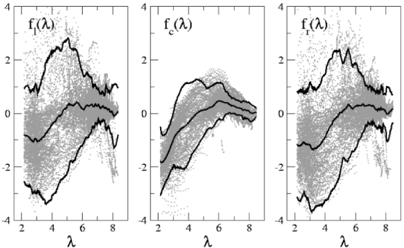
Figure 8: Plot of the functions $f_{l},\,f_{c},\,f_{r}$ with pointwise standard deviations (black lines) on top of the partial residuals (grey dots). The left and right functions show wide scatter, reflected in the individual correlations (numbers are given in the text). The curves display the expected convex shape. For small ripple length there is a systematic deviation in the left and right function.

In Fig. 9 the left, center and right function are plotted together. Encouragingly, with respect to the established model, the functions fall close together except for small ripple lengths. The model has been developed in the region close to the final length, thus the result confirms the model. For small lengths, the result should be considered as input for further modeling. In the case of small ripple lengths, the deviations of the side functions to the center indicate that in the small ripple length region, a difference between center and sides exists. If one averages over left, center and right function, assuming that all three functions are equal and differences arise from measurement errors one obtains the thick black line in Fig. 9.

The model has been obtained as a great simplification of the highly complex granular-fluid system. Given additionally a certain amount of measurement and numerical errors from data processing, one can say that the model is well confirmed by direct, nonparametric data analysis. Further activity aims at a more general modeling in the sense of Eq. (14) to check if there are differences in the interaction functions of the sides and the center which is theoretically very improbable. The direct justification of the model (17) is a success not only for the modeler but as well for statistical data analysis in physical experiments.

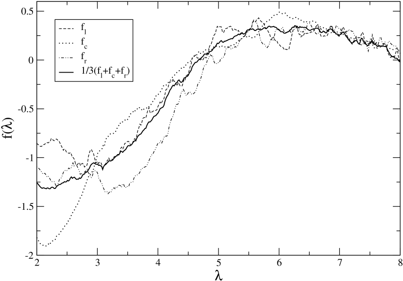
Figure 9: Results from averaging over different runs ($f_{l},f_{c},f_{r}$). For long ripple lengths -the regime, the model has been developed for- one observes a very good coincidence. Theoretically, a difference between sides and center is not expected; assuming them to be equal, averaging yields the black line as an estimation for the true interaction function.

5 Discussion and conclusion

Some of the facts about generalized additive models, backfitting algorithms and ACE have been presented. With a step by step explanation the basic ideas of algorithms and some technical details have been discussed. In the examples, problems with nonlinear transformation of data have been pointed out and the effect of additional, uncorrelated variables has been investigated. With data from an example for a complex pattern forming system, it has been shown how to apply the algorithms to spatio-temporal data and explained the main difficulties for applications. With data analysis a simple model has been validated, which has been developed by physical arguments and coarse graining of the highly complex system of underwater vortex ripples.

Generalized additive models occur often in physical and engineering applications. The idea to obtain models directly from data can be realized with the techniques developed in statistical science. The focus of the presented methods lies in the possibility to determine nonlinearities. Results from the nonparametric data analysis help the theoretician to improve analytical models as well as the applied physicist or engineer who just needs a working model to represent the system dynamics. These aspects can be closed to a circuit - measurement - data analysis - theoretical modeling - which can be iterated until a consistent model for the system under consideration is obtained. It can be expected that the use of nonparametric methods is helpful as well in situations where little is known about the system. There, working models can be inferred without further theoretical justification but as tools

While in this article additive models have been, there exist techniques to solve for either additive or multiplicative models, e.g. the marginal integration [28] or alternatively Breimans $\Pi$-method [29] (without a claim for completeness). Implementations of the backfitting procedure or the ACE algorithm exist for the S-PLUS language or the public domain clone R-PLUS, or in the worldwide web [30].

Statistical approaches are promising tools for the analysis of complex systems, since nonlinearities are automatically fetched. Bayesian formulations promise to yield better error models and another, future application can be stochastic modeling, finding a representation of the residuals in form of a noise term with measured probability distribution.

6 Acknowledgements

I thank K. Andersen, J. Kurths, A. Pikovsky and A. Politi for support and discussion, a special thanks to H. Voss who led my attention to this kind of problems. F. Schmidt has provided computer wisdom, L. Barker-Exp. was a constant source of inspiration. I acknowledge support by the DFG (German research foundation), project number PI 200/7-01.

References

- [1] T. Hastie and R. Tibshirani. Generalized additive models. Stat. Sci., 1:295–318, 1986.
- [2] T.J. Hastie and R.J. Tibshirani. Generalized Additive Models. Chapman and Hall, London, 1990.
- [3] H. Kantz and T. Schreiber. Nonlinear time series analysis. Cambridge University Press, 1997.
- [4] E. Ott, T. Sauer, and J.A. Yorke. Coping with Chaos. Series in Nonlinear Science. Wiley, New York, 1994.
- [5] B P. Flannery S. A. Teukolsky, W. T. Vetterling. Numerical Recipes in C: The Art of Scientific Computing. Cambridge University Press, Cambridge, 2nd edition, 1993.
- [6] D. C. Montgomery. Introduction to linear regression analysis. Wiley, New York, 1992.
- [7] W. Härdle and P. Hall. On the backfitting algorithm for additive regression models. Cambridge University Press, Cambrige, 1993.
- [8] A. Buja, T.J. Hastie, and R.J. Tibshirani. Linear smoothers and additive models. Ann. Stat., 17(2):453–555, 1989.
- [9] L. Breiman and J.H. Friedman. Estimating optimal transformations for multiple regression and correlation. J. Am. Stat. Assoc., 80:580–598, 1985.
- [10] J. Honerkamp. Stochastic dynamical systems. VCH, New York, 1994.
- [11] J. Fan and Y.K. Truong. Nonparametric regression with errors in variables. Ann. Stat., 21(4):1900–1925, 1993.
- [12] R.J. Carroll, J.D. Maca, and D. Ruppert. Nonparametric regression in the presence of measurement error. Biometrika, 86(3):541–554, 1999.
- [13] E. Mammen, O. Linton, and J. Nielsen. The existence and asymptotic properties of a backfitting projection algorithm under weak conditions. Ann. Statist., 27(5):1443–1490, 1999.
- [14] T. Hastie and R. Tibshirani. Bayesian backfitting. Stat. Sci., 15(3):196–223, 2000.
- [15] A. Buja. Remarks on functional canonical variates, alternating least squares methods and ACE. Ann. Stat., 18(3):1032–1069, 1990.
- [16] A. Rényi. On measures of dependence. Acta. Math. Acad. Sci. Hungar., 10:441–451, 1959.
- [17] C.B. Bell. Mutual information and maximal correlation as measures of dependence. Ann. Math. Stat., 33:587–595, 1962.
- [18] P. Csaki and J. Fischer. On the general notion of maximal correlation. Magyar Tud. Akad. Mat. Kutato Int. Kozl., 8:27–51, 1963.
- [19] A. Rényi. Probability theory. Akadémiai Kiadó, Budapest, 1970.
- [20] J. Lambert. Computational Methods in Ordinary Differential Equations. Springer, New York, 1973.
- [21] P.J. Mitchell and D.F. Griffith. The finite difference method in partial differential equations. Wiley, New York, 1980.
- [22] C. Canuto, M.Y. Hussaini, A. Quarteroni, and T.A. Zang. Spectral methods in fluid dynamics. Springer, New York, 1988.
- [23] M.C. Cross and P.C. Hohenberg. Pattern formation outside equilibrium. Rev. Mod. Phys., 65:3, 851-1112.
- [24] M. Abel H. Voss, P. Kolodner and J. Kurths. Amplitude equations from spatiotemporal binary-fluid convection data. Phys. Rev. Lett., 83(17):3422–3425, 1999.
- [25] K.H. Andersen, M.L. Chabanol, and M. v. Hecke. Dynamical models for sand ripples beneathe surface waves. Phys Rev. E, 63(6):66308, 1999.
- [26] K.H. Andersen, M. Abel, J. Krug, C. Ellegaard, L.R. Soendergaard, and J. Udesen. Pattern dynamics of vortex ripples in sand: Nonlinear modeling and experimental validation. Phys. Rev. Lett., 88(23):4302, 2002.
- [27] J. L. Hansen, M. van Hecke, A. Haaning, C. Ellegaard, K. H. Andersen, T. Bohr, and T. Sams. Instabilities in sand ripples. Nature, 410:324, 2001.
- [28] O. Linton and J.P. Nielsen. A kernel method of estimating structured nonparametric regression based on marginal integration. Biometrika, 82(1):93–100, 1995.
- [29] L. Breiman. The method for estimating multivariate functions from noisy data. Technometrics, 33(2):125–143, 1991.
-
[30]
http://www.gnu.org/directory/Mathematics/Statistics,
http://www.splus.com,
http://www.stat.physik.uni-potsdam.de/markus/download,.