Scaling and the prediction of energy spectra in decaying hydrodynamic turbulence

Abstract

Few rigorous results are derived for fully developed turbulence. By applying the scaling properties of the Navier-Stokes equation we have derived a relation for the energy spectrum valid for unforced or decaying isotropic turbulence. We find the existence of a scaling function $\psi$. The energy spectrum can at any time by a suitable rescaling be mapped onto this function. This indicates that the initial (primordial) energy spectrum is in principle retained in the energy spectrum observed at any later time, and the principle of permanence of large eddies is derived. The result can be seen as a restoration of the determinism of the Navier-Stokes equation in the mean. We compare our results with a windtunnel experiment and find good agreement.

The Navier-Stokes equation (NSE) for hydrodynamic flow has been known for many years, and several interesting numerical results have been found. However, very few analytic statements have been derived from these equations [1, 2]. In this Letter we consider decaying isotropic turbulence, i.e. hydrodynamics without external forcing.

One well known feature of the hydrodynamic equations is their invariance under re-scaling when the coordinates are scaled by an arbitrary quantity $l$. Any solution to the NSE can then be mapped onto another solution with a corresponding change in the velocity, the time and the diffusion coefficient $\nu$. The same scaling argument applies to the energy density. In the following we shall show that this leads to a general scaling behavior of the energy density considered as a function of $k,t,\nu$.

The result resembles the $k^{4}$ backscattering at integral scales obtained in EDQNM closure calculations [3]. In studies of the decay of homogeneous and isotropic turbulence self-similarity in the shape of the energy spectra are often assumed, expressed as the principle of permanence of large eddies (PLE)[2]. In a recent interesting phenomenological study it was proposed that for initial spectra not as steep as $k^{4}$ there will be three ranges of self-similarity where PLE only applies to the very large scales [4].

We shall now derive the scaling properties of the energy density directly from the scaling properties of the NSE. This has been done by one of the authors in the case where viscosity was ignored [5]. Here we shall generalize these results. Consider the energy density in $D$ dimensions, given by

$${\cal E}(k,t,\nu,K,L)=$$ (1)

$$\frac{\Omega_{D}k^{D-1}}{(2\pi)^{D}L^{D}}\int_{1/K}^{L}d^{D}xd^{D}y~{}e^{i{\bf k(x-y)}}\langle{\bf v(x},t){\bf v(y},t)\rangle,$$ (2)

where $L$ and $K$ are infrared and ultraviolet cutoffs, respectively, and $\Omega_{D}$ is the solid angle. We assume isotropy such that the energy density only depends on the modulus $k=|{\bf k}|$ of the wave vector. The total energy density is given by

$$E(t) = \int_{1/L}^{K}dk\,{\cal E}(k,t,\nu,L,K)$$ (3)

$$= \frac{1}{2}~{}\int_{1/K}^{L}d^{D}x\,\langle{\bf v(x},t)^{2}\rangle.$$ (4)

Using the invariance of the unforced NSE under the scaling

$${\bf x}\rightarrow l{\bf x},~{}~{}t\rightarrow l^{1-h}t,~{}~{}{\bf v}\rightarrow l^{h}{\bf v},~{}~{}\nu\rightarrow l^{1+h}\nu,$$ (5)

where $h$ is an arbitrary parameter, the relation

$${\cal E}(k/l,l^{1-h}t,l^{1+h}\nu,K/l,Ll)=l^{1+2h}{\cal E}(k,t,\nu,K,L)$$ (6)

trivially follows.

In the following we assume the cutoffs such that for the relevant physical range we have $1/L\ll k\ll K$. We will therefore suppress the explicit dependence of the energy density on the cutoffs. The viscosity provides a physical cutoff for large $k$ while the cutoff $1/L$ is determined by the boundary conditions at the integral scale.

Let us simplify (6) by introducing the new function $\psi$ by defining

$${\cal E}(k,t,\nu)=k^{q}~{}\psi(k,t,\nu).$$ (7)

In the above equations we introduced the quantity $q=-1-2h$, which will be used in the following. To get more information, consider the relation (6) as a function of $l$, differentiate with respect to $l$, and put $l=1$ afterward. This yields the differential equation

$$-\frac{\partial\psi}{\partial\ln k}+{\textstyle\frac{q+3}{2}}\frac{\partial\psi}{\partial\ln t}+{\textstyle\frac{1-q}{2}}\frac{\partial\psi}{\partial\ln\nu}=0.$$ (8)

The general solution of this equation can be written in different equivalent forms:

$$\psi(k,t,\nu)=$$ (9)

$$F_{\gamma}({\textstyle\frac{q+3}{2}}\ln k+\ln t,{\textstyle\frac{(q+3)+(1-q)\gamma}{2}}\ln k+\ln t+\gamma\ln\nu)$$ (10)

where $F_{\gamma}$ is an arbitrary function, and $\gamma\neq 0$ is an arbitrary constant. These solutions correspond to

$${\cal E}(k,t,\nu)=k^{q}~{}\psi_{1}\left(k^{\frac{3+q}{2}}t,\nu t^{-\frac{1-q}{3+q}}\right),$$ (11)

for $\gamma=-(q+3)/(1-q)$ or

$${\cal E}(k,t,\nu)=k^{q}~{}\psi_{2}\left(k^{\frac{3+q}{2}}t,\nu k^{2}t\right),$$ (12)

for $\gamma=1$. This is the main result of this Letter, the consequences of which we will describe in the following.

If we take $t=0$ as the initial time, then the initial spectrum is immediately obtained as a power $k^{q}$ as stated before (assuming that $\psi\neq 0$ for $t=0$). If the cutoffs $L,K$ had been explicitely included, they would appear as additional arguments $kL$ and $k/K$ in (11) and (12).

If we simplify by assuming a very high Reynolds number flow with a developed inertial range, then diffusion can be ignored for $k$ and $t$ sufficiently small such that the energy spectrum should have the form

$${\cal E}(k,t,\nu)\approx k^{q}~{}\psi\left(k^{\frac{3+q}{2}}t\right).$$ (13)

Note that this corresponds to a solution (10) with $\gamma=0$. It is clear that in general the spectrum remembers the initial spectrum through the factor in front of $\psi$, the scaling variable $k^{(3+q)/2}t$ and the functional form of $\psi$. The quantity $k^{(3+q)/2}t$ is invariant under the rescaling (5) with the power $h=-(1+q)/2$. We must stress here that (13) is only valid as a ’local in spectral space’ approximation. Integrating (13) to obtain the total energy lead, as will be elaborated later, to an inconsistency.

Shiromizu [6] has shown from renormalization group arguments that (13) emerges after long time, due to the existence of a fixed point.

From the scaling argument the actual form of the function $\psi(x)$ cannot be found. If we impose the boundary condition that the Kolmogorov spectrum should appear for large $k$’s and/or $t$, we must have

$$\psi(x)\sim x^{-2\frac{5+3q}{3(3+q)}},~{}~{}x=k^{\frac{3+q}{2}}t,~{}~{}~{}{\rm(3D)},$$ (14)

for large values of $x$. This leads to

$${\cal E}\sim k^{-5/3}~{}t^{-2\frac{5+3q}{3(3+q)}}.$$ (15)

For even larger values of $x$ diffusion would of course become important. Now from classical K41 [7] dimensional counting we have ${\cal E}\sim k^{-5/3}\epsilon^{2/3}$, where $\epsilon=dE/dt$ is the mean energy dissipation. Comparing with (15) we have $dE/dt\sim t^{-(5+3q)/(3+q)}$ which after integration gives

$$E\sim t^{-2(1+q)/(3+q)}.$$ (16)

Note that for $q\leq-1$ and $\psi(0)>0$ we get from (13) an infrared divergency in the total energy. This reflects itself in an unphysical growth of the energy with time, so for $q\leq-1$ (16) must be modified by an explicit dependence on the cutoff $1/L$.

In 2D one expects the energy density to behave like $k^{-3}$, which corresponds to

$$\psi(x)\sim x^{-2},~{}~{}~{}{\rm(2D)},$$ (17)

for large values of $x$. This gives

$${\cal E}\sim k^{-3}t^{-2}$$ (18)

for all $q$ except $q=-1$, where ${\cal E}=k^{-3}\psi(t)$.

The interpretation of the scaling as giving the development of an initial power spectrum is of limited interest in practice. In the following we shall therefore show that it is possible to use the scaling to obtain simple relations between the energy densities at different times, allowing any “initial” spectrum compatible with NS without forcing. Let us assume that the spectrum has been measured (or is otherwise known) at a time $t_{0}\neq 0$. From the scaling we then obtain

$${\cal E}_{0}(k,\nu)\equiv{\cal E}(k,t_{0},\nu)=k^{q}~{}\psi_{1}\left(k^{\frac{3+q}{2}}~{}t_{0},\nu~{}t_{0}^{-\frac{1-q}{3+q}}\right).$$ (19)

We do not assume any special form for the initial energy density ${\cal E}_{0}$. From the point of view of the scaling argument, the quantity $q$ is an arbitrary parameter. Later we shall explain how to determine $q$ for a given spectrum.

The relation (19) can be used to construct the $k-$dependence of the scaling function from the measured ${\cal E}_{0}$ by a simple shift of variables,

$$\psi_{1}\left(k^{\frac{3+q}{2}}~{}t,\nu~{}t_{0}^{-\frac{1-q}{3+q}}\right)=$$ (20)

$$k^{-q}~{}\left(t/t_{0}\right)^{-\frac{2q}{3+q}}~{}{\cal E}_{0}\left(k~{}\left(t/t_{0}\right)^{\frac{2}{3+q}},\nu\right).$$ (21)

This in turn leads to the following relation between the energy densities at different times,

$${\cal E}\left(k,t,\nu~{}\left(\frac{t_{0}}{t}\right)^{\frac{1-q}{3+q}}\right)=\left(\frac{t_{0}}{t}\right)^{\frac{2q}{3+q}}~{}{\cal E}_{0}\left(k~{}\left(\frac{t}{t_{0}}\right)^{\frac{2}{3+q}},\nu\right).$$ (22)

This relation is a rewriting of the basic equation (4). It is an expression of what could be called determinism in the mean in decaying turbulence, which indeed is not predictable in time. We see that in spite of the chaotic behavior of the velocity, it is in principle possible to predict the energy density from knowing it at a fixed time. This predictive power is strongest in a region where diffusion can be ignored. Otherwise (22) makes predictions of the energy densities for different times and different viscosities, and relevant experiments may be hard to carry out in practice.

On the right hand side of (22) the time dependence of the argument proportional to $\nu$ is absent for $q=1$ and is very weak for $q$ not too far from 1. In the application to be discussed below we see no effect of diffusion, except for large $k$.

The scaling arguments leading to the above results are based on a scaling of the time by a positive quantity. Taking time itself to be positive, it follows that the earliest time we can have is $t=0$. We shall now discuss how the parameter $q$ can be determined in principle. In doing this we consider the high Reynolds number limit by taking $\nu\rightarrow 0$ (for $q=1$ this is not necessary). Then (22) reduces to

$${\cal E}(k,t,\nu\rightarrow 0)=(t_{0}/t)^{\frac{2q}{3+q}}~{}{\cal E}_{0}\left(k~{}(t/t_{0})^{\frac{2}{3+q}},\nu\rightarrow 0\right).$$ (23)

In the limit $t\rightarrow 0$ existence of the spectrum on the left hand side requires

$${\cal E}_{0}\left(k~{}(t/t_{0})^{\frac{2}{3+q}},\nu\rightarrow 0\right)\sim\left(k(t/t_{0})^{\frac{2}{3+q}}\right)^{q}.$$ (24)

In (23) this implies

$${\cal E}(k,t,\nu\rightarrow 0)\sim k^{q}~{}~{}~{}{\rm for}~{}~{}t\rightarrow 0.$$ (25)

Thus we see that irrespective of whether the spectrum is measured at the initial time, it must behave like $k^{q}$ at the earliest possible time, in the limit $\nu\rightarrow 0$, which means that $k$ should not be too large. Even if the experiment was not operative at $t=0$, one can extrapolate back to a hypothetical initial time $t=0$.

From (24) it also follows that

$${\cal E}(k,t,\nu\rightarrow 0)\sim k^{q}~{}~{}{\rm for}~{}~{}k\rightarrow 0.$$ (26)

Thus, for all times the spectrum keeps its original form for very low values of $k$. This is the principle of permanence of large eddies. It allows us to fix the parameter $q$ if experimental results exist for sufficiently small $k$ by fitting the data to $k^{q}$. It should be noticed that we have only been able to prove the principle of permanency of large eddies when $\nu\rightarrow 0$, except for the case $q=1$, where $\nu$ is not mixed up with the time in (22). A weaker assumption used in the proof is the existence of the spectrum for $t\rightarrow 0$, which imposes the boundary condition (24) on ${\cal E}_{0}$.

In order to test these results consider the experimental measurements of the energy spectrum in decaying turbulence by Comte-Bellot and Corrsin [8]. The energy spectrum was measured in a windtunnel experiment at different distances from the turbulence generating grid, see the figure (a) and (d)). The scaling parameter $q$ is determined from the data by using (16). It is found that $E(t)\sim t^{-1.4}$ which is in the range of most experimental findings [9]. In panels (b) and (e) this is done and from the scaling we obtain in both cases $q=3.67$. The panels (c) and (f) show the scaling function $\psi(k^{(3+q)/2}t)={\cal E}(k,t,\nu)/k^{q}$ obtained from (13) as a function of $(k^{(3+q)/2}t)^{2/(3+q)}$. The collapse is seen to be perfect. The energy spectra show an inertial range of less than two decades, and even less for the 1 inch grid experiment. So even in this case of relatively low Reynolds number flow the dependence of the scaling function on $\nu$ is weak and (13) holds very well. It should, furthermore, be noticed that the factor $(t/t_{0})^{(1-q)/(3+q)}$, which multiplies $\nu$ in (22) for these experiments vary from 1 to 0.42, i.e. by a factor less than 2.4. That could as well be the reason why the dependence on $\nu$ can not be detected in the experimental data.

In general, the energy cannot be obtained by integration over the energy density, unless one has some knowledge of the scaling function $\psi$. For example, without such knowledge one cannot judge the convergence of the relevant integral. In the case $q=1$ the situation is, however, quite different, since (11) shows that

$${\cal E}(k,t,\nu)=k~{}\psi_{1}\left(k^{2}t,\nu\right)\equiv k~{}\psi\left(k^{2}t\right),$$ (27)

where we left out any explicit reference to the diffusion coefficient since it is the same on both sides. In principle, this equation can be tested experimentally as a check of the validity of the NSE.

Consider now the total energy,

$$E(t)=\int_{0}^{\infty}dk~{}k\psi(k^{2}t)=\frac{1}{2t}~{}\int_{0}^{\infty}dy~{}\psi(y),$$ (28)

which shows that in the case $q=1$ the NSE predict a $1/t$ decay of the total energy. Since diffusion is included the integral is expected to converge rapidly. The inertial range, where the energy is constant, would be defined by introducing a cutoff $y_{0}(t)$ on the $y-$integral. Then one should require

$$\int_{0}^{y_{0}(t)}dy~{}\psi(y)\propto t$$ (29)

The Kolmogorov scale $y_{0}(t)$ can of course only be determined from knowledge of the function $\psi$. In order to obtain the energy in cases with $q\neq 1$, one would also need some knowledge of the scaling function. The classical problem of assuming a scaling relation of the form (13) where the diffusion is ignored all together is illuminated by considering the requirement of energy conservation. This leads to the exact relation

$$\frac{dE}{dt} = \frac{d}{dt}\int_{0}^{\infty}dk~{}{\cal E}(k,t)$$ (30)

$$= -2\nu\int_{0}^{\infty}dk~{}k^{2}{\cal E}(k,t).$$ (31)

Using (11) after a shift of integration variable this can be expressed as

$${\textstyle\frac{2(1+q)}{(3+q)^{2}}}\int_{0}^{\infty}dx~{}x^{\frac{q-1}{3+q}}~{}\psi_{1}(x,z)$$ (32)

$$+ {\textstyle\frac{1-q}{3+q}}\int_{0}^{\infty}dx~{}x^{\frac{q-1}{3+q}}~{}z\partial_{z}\psi_{1}(x,z)=2z\int_{0}^{\infty}dx~{}x\psi_{1}(x,z),$$ (33)

where the variable $x$ is defined in (14) and $z=\nu~{}t^{-\frac{1-q}{3+q}}$ For $q=1$ this simplifies to

$$\int_{0}^{\infty}dx~{}\psi_{1}(x,\nu)=2\nu\int_{0}^{\infty}dx~{}x\psi_{1}(x,\nu).$$ (34)

This relation gives a rather weak constraint on the scaling function. It is now seen why the second argument in $\psi_{1}$ cannot be ignored: For $q\neq 1$ (32) cannot be satisfied, since this would lead to the meaningless requirement $t^{(q-1)/(3+q)}=$constant. However, when the argument $z$ is included there is no such problem, since all terms in (32) are $z-$dependent.

Eq. (34) simply states that $\langle x\rangle=1/(2\nu)$. Thus, the mean value of the scaling variable is determined by the diffusion, and $\langle k^{2}\rangle=1/(2\nu t)$. Thus, for large times, the mean value moves toward small $k$, as expected, with a rate given by $\nu$. In a similar way we can analyze the content of (32). Defining the quantity

$$\langle\langle x^{\alpha}\rangle\rangle=\int_{0}^{\infty}dx~{}x^{\alpha}~{}\psi_{1}(x,z),$$ (35)

then (32) has the solution:

$$\langle\langle k^{(q-1)/2}\rangle\rangle/\langle\langle k^{(3+q)/2}\rangle\rangle=\mbox{const.}\nu t.$$ (36)

This can be interpreted by introducing a weight function $w(k)=k^{(q-1)/2}$, from which we obtain

$$\langle k^{2}\rangle_{w}\sim 1/\nu t,$$ (37)

so $k$ approaches zero as time goes by, with a rate again given by $\nu$. It is interesting to note that (37) behaves exactly as a spectral diffusion.

To summarize, we have derived a rigorous scaling relation in the case of decaying hydrodynamic turbulence with a given initial state. This is expressed in terms of the function $\psi$ which itself is not a power function, but depends on the initial scaling. This means that the information of the primordial state is still on average present at later times. The information travels from the small scales to the large scales (or backwards in $k$-space) in a diffusive way.

Useful comments from E. Aurell, G. Eyink and V. Yakhot are gratefully acknowledged.

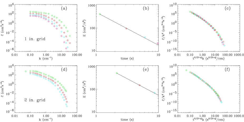
FIG. 1.: Decay of grid generated turbulence in a windtunnel (Comte-Bellot and Corrsin, 1971)Panels (a) and (d) show energy spectra in two experiments with grid spacing of 1 inch and 2 inches respectively. The kinematic viscosity is that of air, $\nu=1.5\times 10^{-5}~{}m^{2}/s$. The spectra are measured at different distances from the grid, which by Taylors hypothesis is converted into times using $t=D/U_{0}$, where $D$ is the distance from the mesh and $U_{0}$ is the wind velocity upstream from the grid. The times are in panel (a): t=1.14 s (green), t=3.05 s (red), t=6.1 s (blue), t=9.8 s (purple), and in panel (d): t=1.07 s (green), t=2.49 s (red) and t=4.34 s (blue). Panels (b) and (e) show the total energy $E(t)$ as a function of time $t$ with the color coding as in panels (a) and (d). The straight lines are $E\sim t^{-2(1+q)/(3+q)}$ with $q=3.67$. Panels (c) and (f) show the scaling function $\psi(k^{(3+q)/2}t)={\cal E}(k,t,\nu)/k^{q}$ as a function of $kt^{2/(3+q)}$ with $q=3.67$.

REFERENCES

- [1] A.S. Monin and A.M. Yaglom, “Statistical Fluid Mechanics: Vol. I, II”, MIT Press, Cambridge Mass., (1975)
- [2] U. Frisch, “Turbulence: The legacy of A.N. Kolmogorov”, Cambridge University Press, Cambridge, (1995)
- [3] M. Lesieur, ”Turbulence in Fluids, Third Revised and Enlarged Edition”, Kluwer Academic Publishers, (1997)
- [4] G. L. Eyink and D. J. Thomson, Phys. Fluids, 12, 477, (2000)
- [5] P. Olesen, Phys. Lett. B 398, 321, (1997)
- [6] T. Shiromizu, Phys. Lett. B 443, 127, (1998)
- [7] A. N. Kolmogorov, Dokl. Akad. Nauk SSSR, 31, 538, (1941)
- [8] G. Comte-Bellot and S. Corrsin, J. Fluid Mech., 48, 273, (1971)
- [9] M. S. Mohamed and J. C. LaRue, J. Fluid Mech., 219, 195, (1990)