Survival and Extinction in Cyclic and Neutral Three–Species Systems

We study the $ABC$ model ($A+B\rightarrow 2B$, $B+C\rightarrow 2C$, $C+A\rightarrow 2A$), and its counterpart: the three–component neutral drift model ($A+B\rightarrow 2A$ or $2B$, $B+C\rightarrow 2B$ or $2C$, $C+A\rightarrow 2C$ or $2A$.) In the former case, the mean field approximation exhibits cyclic behaviour with an amplitude determined by the initial condition. When stochastic phenomena are taken into account the amplitude of oscillations will drift and eventually one and then two of the three species will become extinct. The second model remains stationary for all initial conditions in the mean field approximation, and drifts when stochastic phenomena are considered. We analyzed the distribution of first extinction times of both models by simulations of the Master Equation, and from the point of view of the Fokker-Planck equation. Survival probability vs. time plots suggest an exponential decay. For the neutral model the extinction rate is inversely proportional to the system size, while the cyclic model exhibits anomalous behaviour for small system sizes. In the large system size limit the extinction times for both models will be the same. This result is compatible with the smallest eigenvalue obtained from the numerical solution of the Fokker-Planck equation. We also studied the behaviour of the probability distribution. The exponential decay is found to be robust against certain changes, such as the three reactions having different rates.

1 Introduction

Cyclic phenomena are often ignored when studying epidemiological and evolutionary processes, but nevertheless they can have important consequences, e.g. we contract most infective diseases only once in our lifetime, because our immune system has “memory”. Vaccines are designed based on this knowledge, and they work quite efficiently. However, it is widely accepted that some viruses, such as the flu virus, mutate in order to make themselves unrecognizable by our immune system, and thus be able to reinfect us. Immunity to pertussis (whooping cough) is temporary, and decreases as the time after the most recent pertussis infection increases. The chicken pox (agent VZV—varicella zoster virus) also repeats, because immunity wanes with time. Our model is motivated by this type of situation.

In epidemiological models populations are often categorized in three states: susceptible $(S)$, infected $(I)$ and recovered $(R)$. There exists a vast literature about the so-called $SIR$ models, where the “loss of immunity” step is not considered (e.g. the classic texts by Bailey [1], Anderson and May [2], the review by Hethcote [3]). We consider the case when the “loss of immunity” step is present, otherwise referred to as $SIRS$ models [4, 5].

Recently it has been shown that many species of bacteria are able to produce toxic substances that are effective against bacteria of the same species which do not produce a resistance factor against the toxin [6, 7]. These bacteria exist in colonies of three possible types: sensitive $(S)$, killer $(K)$ and resistant $(R)$. The killer type produces the toxin, and the resistance factor that protects it from its own toxin, at a metabolism cost. The resistant strain only produces the resistance factor (at a smaller metabolism cost). The sensitive strain produces neither. Clearly, the $S$ colony can be invaded by a $K$ colony, the $K$ can be invaded by $R$, and the $R$ can be invaded by $S$.

In our first model the population is categorized into three “species”: $A$, $B$, $C$, and the rules are such that when an $A$ meets a $B$, it becomes $B$, when $B$ meets $C$, it becomes $C$, when $C$ meets $A$, it becomes $A$. The total population size is conserved. Otherwise this could be seen as a three-party voter model, when the follower of a certain party “converts” a follower of another certain party when they meet.

The reaction is similar to the cyclical “Rock-paper-scissors game”, of which a biological example has been found recently [8, 9]. It is played by the males of a lizard species that exist in three versions: the blue throat male defends a territory that contains one female, the orange throat male defends a territory with many females, and the male with a throat with yellow stripes does not defend his own territory, but can sneak into the territory of the orange males and mate with their females. Hence, a “blue” population can be invaded by “orange” males, while an “orange” population is vulnerable to “yellow” males, who on their turn are at an disadvantage against the “blue” males, who defend their territory very well. Many spatial models that relate to such systems have been built [10, 11, 12, 22].

The second model is a three–component version of the famous Kimura model of neutral genetic drift [15, 16]. In that case, when individual from two species meet, the offspring may be either of the first or the second species, with equal probability.

2 Description of the Model

Consider a system in which three species $A$, $B$, $C$ are competing in a way described by the reaction: $A+B\rightarrow 2B$, $B+C\rightarrow 2C$, $C+A\rightarrow 2A$.

The rate equations for this system will be:

$$N\frac{dA}{dt}=AC-AB$$

$$N\frac{dB}{dt}=BA-BC$$ (1)

$$N\frac{dC}{dt}=CB-CA$$

with $A+B+C=N=$ const. (we assume the rates are the same, in which case a time–rescale will remove them from the equations.) These equations can be rewritten as:

$$N\frac{d}{dt}\ln A=C-B$$

$$N\frac{d}{dt}\ln B=A-C$$ (2)

$$N\frac{d}{dt}\ln C=B-A$$

which leads to the second conservation rule: $ABC=H$ = const.

The above model contrasts with the neutral drift model ($A+B\rightarrow 2A$ or $2B$, $B+C\rightarrow 2B$ or $2C$, $C+A\rightarrow 2C$ or $2A$) for which:

$$\frac{dA}{dt}=\frac{dB}{dt}=\frac{dC}{dt}=0$$ (3)

Assuming that the system is subject to stochastic noise due to Poisson birth and death processes (intrinsic noise) we get the master equation for the cyclic model:

$$\frac{\partial P(A,B,C,t)}{\partial t}=\frac{1}{N}[(A-1)(C+1)P(A-1,B,C+1,t)-ACP(A,B,C,t)+$$

$$+(A+1)(B-1)P(A+1,B-1,C,t)-ABP(A,B,C,t)+$$

$$+(B+1)(C-1)P(A,B+1,C-1,t)-BCP(A,B,C,t)]$$ (4)

For the neutral drift case the master equation is:

$$\frac{\partial P(A,B,C,t)}{\partial t}=\frac{1}{N}[\frac{1}{2}(A-1)(C+1)P(A-1,B,C+1,t)+$$

$$+\frac{1}{2}(A+1)(C-1)P(A+1,B,C-1,t)-ACP(A,B,C,t)+$$

$$+\frac{1}{2}(A+1)(B-1)P(A+1,B-1,C,t)+\frac{1}{2}(A-1)(B+1)P(A-1,B+1,C,t)-$$

$$-ABP(A,B,C,t)+\frac{1}{2}(B+1)(C-1)P(A,B+1,C-1,t)+$$

$$+\frac{1}{2}(B-1)(C+1)P(A,B-1,C+1,t)-BCP(A,B,C,t)]$$ (5)

Now we introduce the “shift” operators, defined by

$$\epsilon_{A}f(A,B,C)=f(A+1,B,C)$$ (6)

and

$$\epsilon^{-1}_{A}f(A,B,C)=f(A-1,B,C)$$ (7)

and likewise for B and C operators. The master equation for the cyclic model now reads:

$$\frac{\partial P(A,B,C,t)}{\partial t}=\frac{1}{N}[(\epsilon_{C}\epsilon^{-1}_{A}-1)AC+(\epsilon_{A}\epsilon^{-1}_{B}-1)AB+(\epsilon_{B}\epsilon^{-1}_{C}-1)BC]P(A,B,C,t)$$ (8)

and for the neutral drift one:

$$\frac{\partial P(A,B,C,t)}{\partial t}=\frac{1}{N}[(\frac{1}{2}(\epsilon_{C}\epsilon^{-1}_{A}+\epsilon_{A}\epsilon^{-1}_{C})-1)AC+(\frac{1}{2}(\epsilon_{A}\epsilon^{-1}_{B}+\epsilon_{B}\epsilon^{-1}_{A})-1)AB+$$

$$+(\frac{1}{2}(\epsilon_{B}\epsilon^{-1}_{C}+\epsilon_{C}\epsilon^{-1}_{B})-1)BC]P(A,B,C,t)$$ (9)

Next we transform to the intensive quantities

$$x=\frac{A}{N},y=\frac{B}{N},z=\frac{C}{N}$$ (10)

We use the system size expansion of Horsthemke and Brenig [17, 18]. However, the notation and style is closer to Van Kampen [19, 20].

The shift operators become

$$\epsilon_{A(B,C)}=\sum_{j}\frac{1}{j!}N^{-j}\frac{\partial^{j}}{\partial x^{j}(y^{j},z^{j})}$$ (11)

$$\epsilon^{-1}_{A(B,C)}=\sum_{j}\frac{-1^{j}}{j!}N^{-j}\frac{\partial^{j}}{\partial x^{j}(y^{j},z^{j})}$$

Further we use the rules of transformation of random variables to define:

$$W(x,y,z,t)=P(A,B,C,t)\cdot N^{3}$$ (12)

Before we go ahead with the expansion, a few comments are necessary. From the rate equations, it is clear that our system does not have one single steady state or limit cycle. Instead, the mean-field solution is completely dependent on the initial conditions, and we do not have a macroscopic solution to expand about, but rather an infinity of neutrally stable cycles (for the competition case) or points (for the neutral model.) The above expansion, otherwise known as Kramers-Moyal expansion, is discussed by van Kampen [19, 20]. It is a risky expansion, and it does not work in most cases, mainly because higher derivatives are not small themselves. Also, with time, large fluctuations may occur, and since our system presents itself as a fluctuations–driven one, it becomes even more important to watch out for this sort of complications. In the case of neutral drift, the second order term is the leading one, so we would expect this Ansatz to work for large system sizes. In the cyclic competition model, the first order term does not drive the system out of the (neutrally) stable trajectories, and again it would be the second order term to essentially determine the fate of the system. So, we set out to investigate the applicability of the Kramers-Moyal expansion to the cyclic competition and neutral drift three-species systems.

We transform the master equation into an equation for $W(x,y,z,t)$ by substituting the expressions for the shift operators in it, and further by grouping together the terms of the same order in $N$. The terms of order $N^{1}$ cancel, and the first terms in the expansion are of order $N^{0}$; keeping only those gives us the first order equation for the cyclic case:

$$\frac{\partial W}{\partial t}=[(\frac{\partial}{\partial x}-\frac{\partial}{\partial z})xz+(\frac{\partial}{\partial y}-\frac{\partial}{\partial x})yx+(\frac{\partial}{\partial z}-\frac{\partial}{\partial y})zy]W$$ (13)

For the neutral drift case the first-order term is identically zero.

The second order term is obtained by considering the terms of order $N^{-1}$ in the expansion of the master equation:

$$\frac{1}{2N}[(\frac{\partial^{2}}{\partial x^{2}}-2\frac{\partial^{2}}{\partial x\partial z}+\frac{\partial^{2}}{\partial z^{2}})xz+[(\frac{\partial^{2}}{\partial x^{2}}-2\frac{\partial^{2}}{\partial x\partial y}+\frac{\partial^{2}}{\partial y^{2}})xy+$$

$$+[(\frac{\partial^{2}}{\partial y^{2}}-2\frac{\partial^{2}}{\partial y\partial z}+\frac{\partial^{2}}{\partial z^{2}})yz]W$$ (14)

and is identical for both cyclic and neutral drift cases.

3 The First Order Term

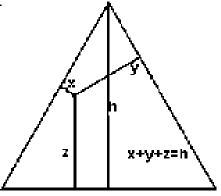
Figure 1: In the equilateral triangle the sum of distances of any point from the sides of the triangle is equal to the height of the triangle (unity.)

The concentrations $x$, $y$, $z$ of a three–component system are commonly represented by the distances of a point inside an equilateral triangle of unit height from its sides (Fig. 1):

For the neutral drift case the first order equation tells us that in the mean–field approximation the system will remain in the initial state forever.

After some algebra, the first order equation [13] for the cyclic system becomes:

$$\frac{\partial W}{\partial t}=\frac{\partial}{\partial x}(xz-xy)W+\frac{\partial}{\partial y}(xy-yz)W+\frac{\partial}{\partial z}(yz-xz)W$$ (15)

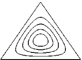
Figure 2: Some of the closed trajectories of the cyclic competition system when only the first order term is considered.

At the centre of the triangle ($x=y=z=1/3$) all three expressions above are zero, so in the first order approximation the system will stay at that state forever. It can be verified that the product $H=xyz$ is a solution of the first-order equation, as is any function of that product. The lines $xyz=$ const. will then represent possible trajectories of the system, which are closed, since there is no term to drive the system out of those trajectories. In this (mean-field) approximation, the cyclic model exhibits global stability with constant system size $N$ [29, 30]. The populations of each species oscillate out of phase with one-another, and the amplitude remains constant [21]. These are the same trajectories that are obtained when one solves the rate equations [1]. Fig. 2 shows some of those closed trajectories.

4 The Second Order Term

The second order term [14], which represents the “diffusion term” must be added to the first order equation to give the Fokker-Planck equation for our system. This term is identical for both the cyclic (competing species) and neutral genetic drift cases. As we will see, this makes the long (evolutionary) time fate of both systems essentially the same, at least for reasonably large system sizes.

The trajectories of a given realisation of the system can easily be obtained by simulation: they initially spiral out of the centre, with the populations of each species oscillating out of phase with one–another, so that the total size of the population is conserved. The amplitude drifts until one of the populations becomes zero (species goes extinct). In other words, the slow second order term makes the system cross from a closed (mean-field) trajectory to a neighbouring one. This would suggest an adiabatic approximation. In the neutral drift model, the fluctuations drive the system from one point–solution of the mean-field equations to a neighbouring one.

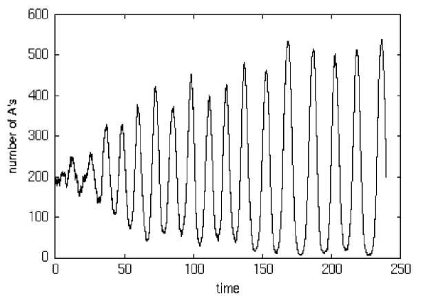
Figure 3: Variation with time of the total number of the $A$ species for a realisation of the cyclic competition system ($N=600$).

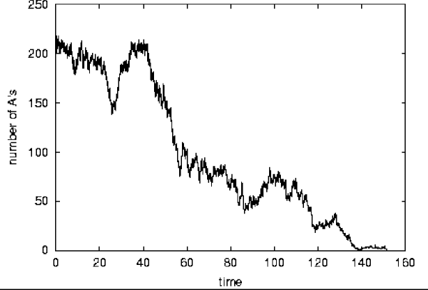
Figure 4: Variation with time of the total number of the $A$ species for a realisation of the neutral drift system ($N=600$).

The computer simulations of both systems start with an equal number of $A$, $B$, $C$, (start at the centre) and generate times for the next possible reaction event with exponential distribution as $-N\cdot\ln(rn)/AB$, (for $A+B\rightarrow 2B$ reaction, and similarly for the other two reactions,) where $rn$ is a random variable with uniform distribution in $[0,1]$ (this means the events are really independent) [23]. The reaction which occurs first is then picked and the system is updated. The process is repeated until one of the species, and then another one, go extinct. Fig. 3 shows the variation with time of the number of $A$ for a realization of the system in the cyclic competition scenario, and Fig. 4 shows the evolution of the number of $A$ population in the neutral drift case (in both realizations the total population size is $N=600$.) From the time series for the population numbers it looks as if the neutral drift model is some sort of “adiabatic” approximation of the cyclic competition model. If in the neutral drift model the population number is random walking, in the cyclic competition one the amplitude of oscillations is random walking! In other words, if we average the cyclic competition model over the cyclic orbits, we get essentially the same behaviour as the neutral drift model. Then the fluctuations drive both models from a neutrally stable cycle (point) to the neighbouring ones, and these fluctuations remain quite small by virtue of the vicinity of the neighbouring cycle (point.) It is quite funny how we all tend to go around in circles in life, even though the point we end up to is still the same!

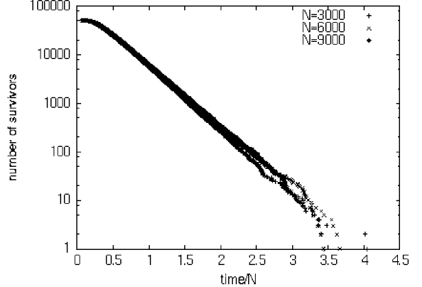
Figure 5: Number of survivors vs. time plots for three different system sizes, same rate cyclic competition case.

We investigated the probability distribution of first extinction times. For that we ran fifty thousands copies of the system for each (different) size of the system, and the number of survivors was plotted vs. time. In the semilog axes we get a straight line, except for the few “rare events”. The slope of this straight line is -3.01 for system size 3000, -2.98 for system size 6000, -2.99 for system size 9000. Fig. 5 shows the plots for these three different system sizes: 3000, 6000, and 9000.

The time dependence of survival probability scales approximately with $1/N$, but there is still a very weak dependence left for small $N$. This can be justified by looking at the Fokker-Planck equation for this system, which contains both a term of order $N^{0}$ and $N^{-1}$.

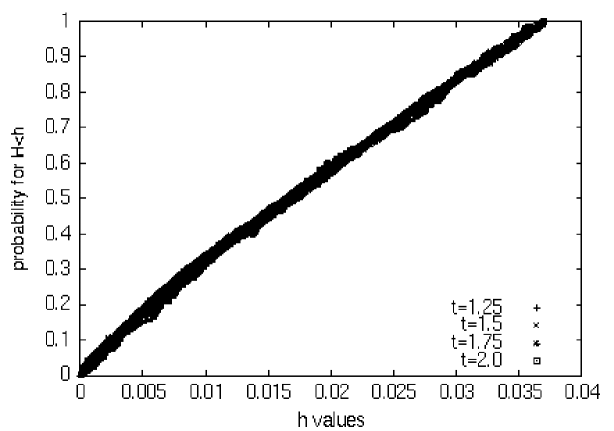
Figure 6: Normalized cummulative probability distribution for the $H=xyz$ quantity for the cyclic competition system at $t=1.25$, $t=1.5$, $t=1.75$, $t=2.0$.

To further investigate the behaviour of the system, we looked at the cummulative, conditional on being alive (which is equivalent to a normalization condition,) probability distribution for $H=xyz$. If $P(H<h|$alive$)$ increases linearly with $H$ for small $H$, the extinction rate will be non-zero, and we will get exponential decay. This corresponds to a constant distribution for $P(H|$alive$)$. Fig. 6 shows these plots for $t=1.25$, $t=1.5$, $t=1.75$, and $t=2.0$ in linear axes.

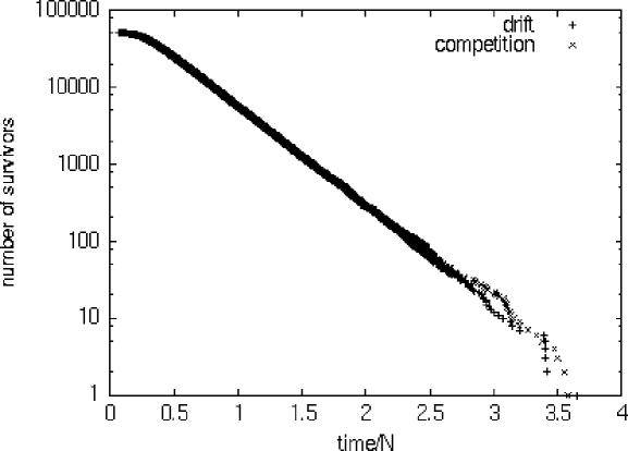
Figure 7: Number of survivors vs. time plots for the cyclic and drift case for system size $N=6000$.

For the neutral drift case the data from the simulations give us a slope of -2.992 for system size 6000, -2.991 for system size 3000. The data collapse when time is rescaled with $1/N$, and that is in agreement with the fact that there is only a term of the order $1/N$ present in the Fokker-Planck equation. In Fig. 7 we show the number of survivors vs. time plots for cyclic (competition) and drift cases together, for system size $N=6000$. They clearly agree.

5 Probability Distribution at Long Times

In order to get an expression for $W$ for long times, we looked at our “experimental” data. It is possible to find a complete set of eigenfunctions of the Laplace equation, which vanish at the boundary. Having this complete set of eigenfunctions for the equilateral triangle [24, 25], the probability density can be written:

$$W=\sum_{m,n}c_{m,n}{\phi}_{m,n}$$ (16)

where ${\phi}_{m,n}$ are the abovementioned symmetric eigenfunctions. The non-normalized eigenfunctions are then obtained from the general expression:

$$\phi_{(m,n)}(x,y)=\sum_{(m,n)}\pm\exp[{\frac{2\pi i}{3}}(nx+my)]$$ (17)

where we are using the relation $x+y+z=1$ and summation over the index pair $(m,n)$ means summation for $(-n,m-n)$, $(-n,-m)$, $(n-m,-m)$, $(n-m,n)$, $(m,n)$, $(m,m-n)$ [25].

We get a symmetric eigenfunction when $m+n$ is a multiple of 3, $m$ is also a multiple of 3, but $m\neq 2n$, and $n\neq 2m$.

In order to calculate the expansion coefficients, we took snapshots of the system at given times, and then used the relation:

$$c_{(m,n)}(t)\propto\frac{1}{p}\sum_{l=1}^{p}{\phi_{(m,n)}(x_{l}(t),y_{l}(t))}$$ (18)

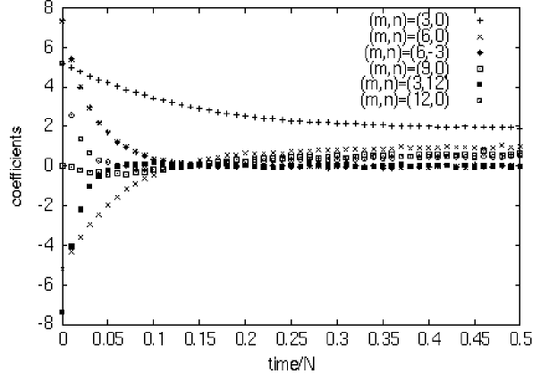
Figure 8: The variation with time of the coefficients for the first six functions in the expansion of $W(t)$: $(m,n)=(3,0)$, $(m,n)=(6,0)$, $(m,n)=(6,-3)$, $(m,n)=(9,0)$, $(m,n)=(3,12)$, $(m,n)=(12,0)$.

where $p$ is the number of experimental points. The time-evolution of the expansion coefficients is given in Fig. 8. The doubly–degenerate functions die out quite soon, while the Lamé symmetric functions persist.

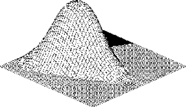
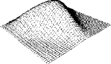
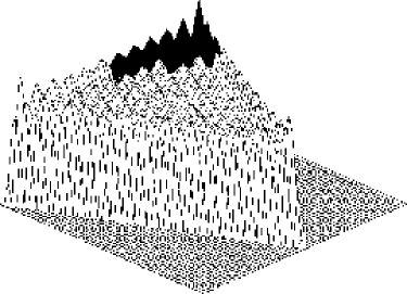
Figure 9: Snapshots at the probability density function at $t=0.1$, $t=0.2$, and $t=1.5$.

With the coefficients obtained this way we can then construct the probability density at different times. Some snapshots at the $W(t)$ are shown in Fig. 9.

At $t=0$ the $W(0)$ is a $\delta$-function. As time passes, for $t=0.1$ we see the $W$ starts to spread, and it spreads even more for $t=0.2$, becoming a “cake” for very long times ($t=1.5$,) for both the cyclic system and the neutral drift one. The “cake” obtained this way shows some Gibbs oscillations, which are due to the inclusion of only a few terms in the expansion, and the presence of the absorbing boundary. For a uniform probability distribution the expansion coefficients are proportional to $1/m$, where $m$ is the first index in the pair $(m,n)$. It can be seen that our “experimental” expansion coefficients approach those values.

The second–order Fokker–Planck equation for the drift case accepts solutions of the form:

$$W(x,y,z,t)=e^{-\lambda t}W(x,y,z)$$ (19)

with $\lambda$ the smallest eigenvalue of the spatial equation. We solved the eigenvalue problem by using the Galerkin method, with the help of Maple, and obtained a value of $\lambda=3.01$ for the smallest eigenvalue, when we keep the first six eigenfunctions in the expansion. This is in very good agreement with our “experimental” data.

6 Case When Rates Are Not the Same

Now consider the cyclic (competition) case when the rates of the three equations are not the same, i. e. the rate equations read like:

$$N\frac{dA}{dt}=c_{13}AC-c_{12}AB$$

$$N\frac{dB}{dt}=c_{21}AB-c_{23}BC$$ (20)

$$N\frac{dC}{dt}=c_{32}BC-c_{31}AC$$

We can always rescale the $A,B,C$ so that the matrix $c_{ij}$ be symmetric, and the equations read:

$$N\frac{dA}{dt}=A(\beta C-\gamma B)$$

$$N\frac{dB}{dt}=B(\gamma A-\alpha C)$$ (21)

$$N\frac{dC}{dt}=C(\alpha B-\beta A)$$

Again, $A+B+C=N=$const. By manipulating the rate equations, we can find the second integral of motion to be $A^{\alpha}B^{\beta}C^{\gamma}=H=$const. The new centre will then be not at the point (1/3, 1/3, 1/3), but at $A=\alpha,B=\beta,C=\gamma$. The lines along which the quantity $A^{\alpha}B^{\beta}C^{\gamma}$ is constant are shown in Fig. 10.

We need to check whether the exponential decay behaviour is universal when the symmetry is broken this way. For this we ran fifty thousand simulations for different combinations of $\alpha$, $\beta$, and $\gamma$, for system size $N=3000$, starting from the new centre ($A=N\cdot\alpha$, $B=N\cdot\beta$, $C=N\cdot\gamma$.) The number of survivors vs. time plots were again obtained, and those plots show that the exponential decay behaviour is robust. The time scale is now dependent on the initial distance from the boundary, with the equal rates case having the largest distance, and so the largest time scale (and the smallest slope.) Some of those plots are shown in Fig. 11. In that figure, the times for the equal rates case (for which the sum of rates is 3) are multiplied by three, to make them comparable to the times for the unequal rates case, for which the sum of rates is 1.

7 Conclusions

We have considered an $ABC$ model in both the cyclic competition and neutral genetic drift versions, and studied the long-term behaviour of such a model. The number of the $A,B,C$ species in the cyclic competition case oscillates with a drifting with time amplitude, until one of the species (and then the next one in the cycle) goes extinct. In the neutral drift case the number of the $A,B,C$ species drifts, until one of them becomes zero. In both scenarios the number of survivors vs. time plots show an exponential decay, with the same exponent. The result is verified by writing and solving the Fokker–Planck equation for the second model. Finally, its robustness is checked against variations in the rate of the three different reactions in the system. It is very interesting to note that there is no difference in the time scale for the ensemble of species in cyclic competition and the case of neutral genetic drift.

There is growing concern about the effects of habitat fragmentation in the survival of the species [13]. If the population of a certain species goes extinct in one patch (e.g. a herd, school, swarm) while it still survives in other patches, then what is known as “rescue effect” can prevent global extinction [14, 26, 27]. Otherwise, the species is doomed to go extinct altogether. The models with individuals of “species” $A$, $B$, and $C$ distributed in a lattice have been studied by Szábo et al. [10, 11, 22]. If we try to model habitat fragmentation as an ensemble of patches, each of those patches can be considered as one copy of our non-spatial system. However, with continuous migration in and out of the patch, the non-spatial picture described in this paper would be seriously perturbed. One aspect of this immigration and emigration has been recently discussed by Togashi and Kaneko [31]. In a first approximation, the broad range of extinction times could relate to the persistence of species that exist in different “versions” such as certain lizards, or even some kinds of bacteria. Applied to its epidemiological scenario, it would relate to the endemicity of certain diseases, namely those with mutating pathogen, and then the outbreaks of epidemics in certain patches (areas). The many patches will then form a network [28]. We have work in progress which places our $ABC$ ensemble in one of these small worlds with a scale-free topology.

8 Acknowledgements

We thank Nicolaas G. van Kampen for constructive criticism, and Michael Döbeli for helpful and interesting discussions and suggestions.

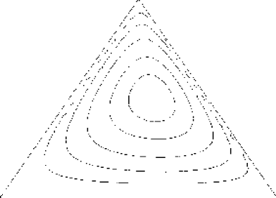
Figure 10: The $H=$const. lines for the case when three reactions happen at different rates. Here $\alpha=$0.2, $\beta=$0.3, $\gamma=$1$-\alpha-\beta=$0.5.

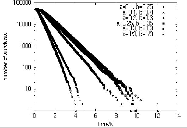
Figure 11: Number of survivors vs. time plots for the unequal rates cyclic competition case for system size 3000 and different combinations of $\alpha$ and $\beta$.

References

- [1] Bailey N. T., The Mathematical Theory of Infectious Diseases, 2nd edition, London: Griffin (1975).
- [2] Anderson R. M. and May R. M., Infectious Diseases of Humans, Oxford University Press, London (1991).
- [3] Hethcote H. W., SIAM Review, 42, 599 (2000).
- [4] Cooke K. L., Calef D. F., and Level E. V., Nonlinear Systems and its Applications, Academic Press, New York, 73 (1977).
- [5] Longini I. M., Mathematical Biosciences, 50, 85 (1980).
- [6] Reeves P., The Bacteriocins, Springer Verlag, New York (1972).
- [7] James R., Lazdunski C., and Pattus F., (editors) Bacteriocins, Microcins and Lantibiotics, Springer Verlag, New York (1991).
- [8] Sinervo B. and Lively C., Nature, 380, 240 (1996).
- [9] Maynard Smith J., Nature, 380, 198 (1996).
- [10] Szabó G., and Czárán T., Phys. Rev. E, 63, 061904 (2001).
- [11] Szabó G., Santos M. A., and Mendes J. F. F., Phys. Rev. E, 60, 3776 (1999).
- [12] Frachebourg L., Krapivsky P. L., and Ben-Naim E., Phys. Rev E, 54, 6186 (1996).
- [13] Pimm S. L., Nature, 393, 23 (1998).
- [14] Blasius B., Huppert A., and Stone L., Nature, 399, 354 (1999).
- [15] Kimura M., and Weiss G. H., Genetics, 49, 561 (1964).
- [16] Weiss G. H., and Kimura M., J. Appl. Prob., 2, 129 (1965).
- [17] Horsthemke W., and Brenig L., Zeitschrift für Physik B, 27, 341 (1977).
- [18] Horsthemke W., Malke-Mansour M., and Brenig L., Zeitschrift für Physik B, 28, 135 (1977).
- [19] Van Kampen N. G., Adv. Chem. Phys. 34, 245 (1976).
- [20] Van Kampen N. G., Stochastic Processes in Physics and Chemistry (revised edition), North-Holland (1997).
- [21] Ruijgrok Th., and Ruijgrok M., J. Stat. Phys., 87, 1145 (1997).
- [22] Szabó G., and Hauert C., Phys. Rev. Let., 89 (11), 118101 (2002).
- [23] Gibson M. A., and Bruck J., J. Phys. Chem. A, 104, 1876 (2000).
- [24] Lamé M. G., Leçons sur le Théorie Mathématique de l’Elasticité des Corps Solides, Paris, Bachelier (1852).
- [25] Pinsky M. A., SIAM J. Math. Anal., 11, 819 (1980).
- [26] Brown J. H., and Kodric-Brown A., Ecology, 58, 445 (1977).
- [27] Earn D. J., Levin S. A., and Rohani P., Science, 290, 1360 (2000).
- [28] Albert R., and Barabási A.-L., Rev. Mod. Phys., 74, 47 (2002).
- [29] Hethcote H. W., Math. Biosci., 28, 335 (1976).
- [30] Hethcote H. W., Three basic epidemiological models, in Applied Mathematical Ecology, L. Gross, T. G. Hallam, and S. A. Levin, eds., Springer-Verlag, Berlin (1989).
- [31] Togashi Y., and Kaneko K., Phys. Rev. Let., 86 (11), 2459 (2001).