Nonlinear dynamics of waves and modulated waves in 1D thermocapillary flows.
I: General presentation and periodic solutions

Abstract

We present experimental results on hydrothermal traveling-waves dynamics in long and narrow 1D channels. The onset of primary traveling-wave patterns is briefly presented for different fluid heights and for annular or bounded channels, i.e., within periodic or non-periodic boundary conditions. For periodic boundary conditions, by increasing the control parameter or changing the discrete mean-wavenumber of the waves, we produce modulated waves patterns. These patterns range from stable periodic phase-solutions, due to supercritical Eckhaus instability, to spatio-temporal defect-chaos involving traveling holes and/or counter-propagating-waves competition, i.e., traveling sources and sinks. The transition from non-linearly saturated Eckhaus modulations to transient pattern-breaks by traveling holes and spatio-temporal defects is documented. Our observations are presented in the framework of coupled complex Ginzburg-Landau equations with additional fourth and fifth order terms which account for the reflection symmetry breaking at high wave-amplitude far from onset. The second part of this paper [1] extends this study to spatially non-periodic patterns observed in both annular and bounded channel.

, ,
and

Introduction

The transition to spatio-temporal chaos in extended non-linear systems remains still today an active field of research. Many studies have been devoted to this problem in the case of stationary spatial patterns and more recently in the case of oscillatory instabilities and non-linear traveling-waves patterns. For example, Rayleigh-Bénard convection [2] and directional viscous fingering [3] in quasi one-dimensional experiments have revealed a transition to spatio-temporal chaos via spatio-temporal intermittency. On the other hand, non-linear traveling-waves have exhibited a fascinating variety of behaviors and patterns. Wave systems have been studied in binary-fluid convection (subcritical traveling waves bifurcation) [4, 5, 6], oscillatory instability in low Prandtl number convection [7, 8], oscillatory rotating convection [9], cylinder wake [10], Taylor dean vortices. [11, 12]

Among these different waves systems, thermocapillary flows and in particular hydrothermal waves [13, 14, 15, 16, 17, 18] or hot wire waves [19, 20, 21, 22] appear as a very simple tool, owing to their supercritical bifurcation. They correspond to the first instability of a thin liquid layer with a free surface subjected to a horizontal temperature gradient [23]. Different experimental configurations have been used to study those traveling waves: rectangular cells with different aspect ratios [13, 24, 25, 18, 15], annular cells [26, 14], cylindrical cells [27, 17] and linear hot wire under the surface of a liquid [19, 20, 21, 22].

Hydrothermal waves provide very interesting systems of traveling waves which can be modeled by envelope equations such as the complex Ginzburg-Landau equation (CGL) [28, 29]. The CGL equation, which describes the large-scale modulations of the bifurcated solutions near oscillatory instabilities, has been extensively studied as shown in a recent review [29]. This situation is due both to its relevance to many experimental systems, even far from threshold, and to the variety of spatio-temporal chaos regimes is exhibits. Theoretical studies and numerical simulations have indeed revealed regimes of phase turbulence [30, 31], amplitude turbulence [30] related to localized defects solutions such as the Bekki-Nozaki or homoclonic holes [32, 33, 34] and, more recently, modulated amplitude waves [35, 36, 37].

Geometries and symetries

We study two different one-dimensional traveling-wave systems: one in an annular geometry and one in a rectangular geometry. The annular setup has periodic boundary conditions and the rectangular setup is finite, bounded with poorly reflecting boundaries. Both are spatially extended. Our results are presented in two companion articles. The present paper begins with a general introduction to the dynamics of hydrothermal waves and its modeling. Then it presents and discuss experimental data in the form of uniform or modulated wave-patterns obtained in the annular cell and corresponding to periodic solutions of the problem. A second paper [1] is devoted to non-periodic and non-uniform patterns, i.e., to patterns either observed in the rectangular bounded channel or observed in the annular channel in cases where the galilean invariance is broken by the presence of fixed defects. The distinction we make between those two classes of experiments is motivated by important differences between the observed wave-patterns. Whereas the present paper I presents results that can be directly connected with numerics or analytics in periodic or infinite systems, this will not the case in paper II, where we will emphasize the convective and absolute regimes and transitions for instabilities. In the following, we will refer to the two papers as I and II and will sometime refer to paper II to provide the reader a broader view on wave-dynamics in actual experiments, where the galilean invariance usually doesn’t hold, which leads to qualitative and quantitative differences from the work presented in the present paper.

The pattern in annular geometry undergoes a supercritical Eckhaus instability in the form of stable traveling modulations [14]. We detail this in the present paper, together with other modulated patterns. We also present realizations of spatio-temporal chaos in our periodic wave-system. We mention similar patterns obtained in rectangular geometry, though their accurate description is given in II.

Outline of the article

This article is segmented as follows: section 1 presents the experimental setups, the main characteristics of hydrothermal waves and CGL modeling. This section is of general interest for the readers of both papers I and II. Section 2 is then devoted to the description of modulated traveling waves in the annulus for a medium fluid height where extensive quantitative measurements have been realized. Section 3 presents additional data about modulated wave patterns observed for smaller fluid heights. Finally, in section 4, we discuss the modulated-wave regimes and develop a comparison with theoretical and numerical solutions.

1 Hydrothermal waves

1.1 Experimental setups

Hydrothermal waves have been studied in two different 1D geometries: annular corresponding to periodic boundary conditions [14] and rectangular corresponding to finite bounded ones [15, 16]. Both geometries consist of a channel with a glass bottom and vertical copper walls filled with a thin layer of silicon oil of viscosity $\nu=0.65$cSt and Prandtl number $P=10$ (see [18] for characteristics of the fluid). The fluid surface is free and a Plexiglas plate is inserted a few millimeters above the surface of the fluid to reduce evaporation.

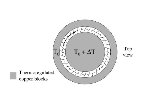
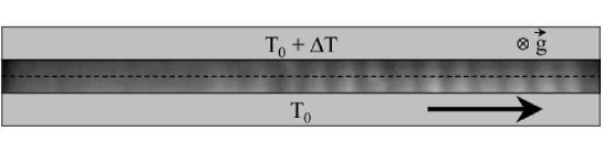
Figure 1: Schematics of the annular periodic channel (top) and rectangular bounded channel (bottom). Traveling hydrothermal waves are represented by a sketch in the annulus and by a photograph in the rectangle. Dashed lines shows the acquisition circle and line respectively.

The annular channel (Fig. 1) is $10$mm wide and its mean radius is $R=80$ mm [14]. The fluid height $h$ is varied between $0.6$ and $3$ mm. The perimeter is $L_{p}=503$ mm which corresponds to an aspect ratio $\Gamma=2\pi R/h=300$ for $h=1.7$ mm. The outer copper wall is cooled by a thermo-regulated fluid circulation at $293$ K while the inner copper block is heated electrically.

The rectangular channel (Fig. 1) is $10$ mm wide and $250$ mm long [13, 18]. Plexiglas blocks are inserted in the channel to reduce the length to $L_{b}=180$ mm, i.e., aspect ratio $\Gamma=L_{b}/h\simeq 100$; this allows us to view the whole cell through a $200$ mm diameter lens. The copper walls are thermo-regulated by fluid circulations.

Let’s define our notation for the channel length: the channel length will be noted $L_{\rm p}$ for the periodic (annular) channel and $L_{\rm b}$ for the bounded (rectangular) channel; without subscript, $L$ will concern the current channel, and $L^{*}$ the non-dimensional length $L/\xi_{0}$, where $\xi_{0}$ stands for the correlation length of the system. $\xi_{0}$ depends of $h$ but not of the channel boundaries (see section 1.3).

Most experiments reported in this paper are performed around $h=1.7$ mm. Otherwise, the height will be noted in text and figure captions. Maintaining the height as constant as possible is a challenge due to evaporation and thermocapillary flow of the oil on the vertical sides of the channels. Height decrease rate is typically $0.1$ mm/h in the rectangular channel and $0.01$ mm/h in the annular channel where more attention has been paid to reduce thermocapillary side-flowing. In some case, the decrease rate has been as low as $0.01$ mm/day. Quantitative data presented below will concern measurements in the range $h=(1.70\pm 0.05)$ mm for the annulus and $h=(1.7\pm 0.1)$ mm for the rectangle.

In both cases thermocouples allow accurate measurements of the temperature difference $\Delta T$ across the channel, typically established with a $\pm 15$mK stability.

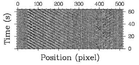
Figure 2: Exemple of unprocessed spatio-temporal diagram of a left traveling wave in the rectangular channel close to onset ($\Delta T=3.8$ K). Only a few periods are presented while usual acquisitions last several hours. The cell is shorter than the acquisition line.

Convective patterns are observed through the glass bottom by shadowgraphy. A parallel vertical white light beam crosses the container from top to bottom and forms a horizontal picture on a screen, mainly due to temperature gradients in the fluid [27, 38, 39]. This configuration insures a low contrast and thus a linear response to the waves. Fig. 1 shows a typical photograph of the wave-pattern in the rectangular channel. Images are digitized with a CCD camera over $512\times 512$ or $768\times 512$ pixels. Spatio-temporal diagrams of 512 data points are then extracted from a line (rectangular geometry) or a circle (annular geometry) and plotted along time (Fig. 2). To extract the pattern behavior from the spatio-temporal diagrams, space and time Fourier transforms and complex demodulation techniques are used. They allow a determination of the local amplitude of the waves, their wavenumber and frequency as detailled in section 1.4.

1.2 hydrothermal waves

The existence of hydrothermal waves in a fluid layer subjected to a horizontal temperature gradient has been predicted on the basis of a linear stability analysis by Smith and Davis [23], and studied numerically in conditions close to our experimental situation by Mercier and Normand [40]. Hydrothermal waves have been detected and characterized in several experiments [13, 18, 24, 25, 41]. In the following, we recall some of their main features obtained in quasi-one-dimensional geometries. More information can be found in Ref. [18].

Given all the physical properties of the fluid, the two parameters which control our experimental system are $h$, the height of fluid in the cell, and $\Delta T$, the horizontal temperature difference between the two walls. The associated dimensionless parameters are:

• the Marangoni number: $Ma=\gamma\Delta Th/\rho\kappa\nu$

• the dynamic Bond number $Bo=\rho g\alpha h^{2}/\gamma$

• the capillary number $Ca=\gamma\Delta T/\sigma$

• the static Bond number $Bd=\rho gh^{2}/\sigma$

where $g$ is the gravitational acceleration, $\alpha$ the thermal expansion coefficient, $\kappa$ the thermal diffusivity, $\rho$ the density of the fluid, $\nu$ the kinematic viscosity, $\sigma$ the surface tension and $\gamma=-(\partial\sigma/\partial T)$. The exact characteristics of the waves depend strongly on these parameters and on the aspect ratios of the containers [18, 24, 42]. For the hydrothermal waves instability considered here, only $Ma$ and $Bo$ are relevant. Moreover, in practice, the experiments reported in this paper are performed with a constant width (10 mm) and for some different fluid depths. Most of the quantitative results concerns $h=1.7$ m. In the following, we will use $\Delta T$ as our control parameter for simplicity.

Figure 3: Stability diagram: critical temperature difference $\Delta T_{c}$ vs. height of liquid $h$ for a $10$ mm width channel. This graph combines data obtained in rectangular ($\circ$) and annular ($\Box$) geometry. BF and HW respectively refer to Basic Flow and Hydrothermal Waves. These data —except for $h=1.7$ mm, see Fig. 4— correspond to the lowest $\Delta T$ where waves are visually seen to occupy the whole cell. These data roughly give the same tendency, schematized by the dashed line.

As soon as $\Delta T\neq 0$, a convective flow is created. The thermal gradient across the cell induces a surface tension gradient on the free surface of the fluid. Due to Marangoni effect ($\gamma>0$), this gradient generates a surface flow towards the cold side, with a bottom recirculation: the basic flow (BF) is a long annular (resp. longitudinal) roll in the annular (resp. rectangular) case. Please note that this basic flow is not due to an instability. However, above a given threshold $\Delta T_{c}$, and for small depth layers $h<h_{r}$ ($h_{r}=2.7$ mm for a $10$ mm width channel), this flow becomes unstable with respect to oblique traveling waves (TW) which propagate along the channel (Fig. 1), i.e., the roll axis [18]. Above $h_{r}$, stationary rolls parallel to the gradient are observed. $\Delta T_{c}$ depends on $h$: when increasing $h$, $\Delta T_{c}$ decreases from small $h$ towards a minimum and then increases up to $h_{r}$ (Fig. 3). As soon as the threshold is crossed, two waves which propagate in opposite direction along the roll axis, and towards the hot wall appear in the container, separated by a source. The source shape as well as the characteristics of the waves and their evolution with time and $\Delta T$ above the threshold depend of $h$.

Figure 4: Amplitude of the hydrothermal waves vs. $\Delta T$ for $h=1.7$ mm and $10$ mm width: experimental data in the annulus with $L_{\rm p}=503$ mm ($\circ$) and in the rectangle with $L_{\rm b}=180$ mm ($\Box$). The annulus data are for patterns with mean wavenumber around the critical wavenumber $k_{\rm c}$, i.e., for $k=54(2\pi/L_{\rm p})$ and $k=55(2\pi/L_{\rm p})$. Solid lines represent fits $A\propto\left(\Delta T-\Delta T_{\rm c}\right)^{1/2}$, $\Delta T_{\rm c}=3.1$K for the annulus (convective threshold) and $A\propto\left(\Delta T-\Delta T_{\rm a}\right)^{1/2}$, $\Delta T_{\rm a}=3.65$K for the rectangle (absolute threshold [15]).

The waves appear via a $I_{\rm o}$ bifurcation [28]: as for a supercritical Hopf bifurcation —but for a spatially extended system— the frequency is finite at threshold and the amplitude of the waves behaves as $(\Delta T-\Delta T_{c})^{1/2}$ [15, 18]. In this paper, we present for the first time the critical amplitude behaviors of supercritical traveling waves in both type of cells: bounded or periodic (Fig. 4). These results are in agreement with the linearity of the shadowgraphic response of our optical system. Please note the difference between the two thresholds presented in Fig. 4: it is due to the difference between the convective and the absolute threshold. It is carefully discussed in the companion paper II. Please note also that finite size effects of order $(2\pi/L)^{2}$ can be neglected in both channel because of large spatial extensions. [15, 42]

In the stability domain of the waves, two types of sources have been evidenced in the rectangular channel [18]. For larger heights, the source is a line and generally evolves towards one end of the container leaving a single wave whereas for smaller heights, the source looks like a point and emits a circular wave which becomes almost planar far from the source in both directions [18, 17]. In the periodic annular channel the two types of sources are also observed, but only during transients; sources and sinks are both unstable near onset always leaving a single wave; this is detailed in section LABEL:sec:sources of II. In the following, we report behaviors obtained for small heights, but the width of the two geometries is small (10 mm) and the waves behavior can still be considered as one-dimensional.

1.3 Complex Ginzburg-Landau envelope equation modeling

The experimental shadowgraphic signal $\theta_{r}(x,t)$ is basically a space- and time-periodic field (Fig. 2). Let’s describe high frequencies with Fourier modes and low-frequency dynamics by two slowly varying amplitudes A and B:

$$\theta_{r}(x,t)=A(X,T)\ \exp i(\omega_{\rm c}t-k_{\rm c}x)$$

$$\mbox{}+ B(X,T)\ \exp i(\omega_{\rm c}t+k_{\rm c}x)+c.c.+...$$ (1)

where $\omega_{\rm c}$ is the critical frequency, $k_{\rm c}$ is the critical wavenumber, c.c. stands for complex conjugate and the dots for harmonics. Near threshold, these slowly varying amplitudes may be described by a system of two complex Ginzburg-Landau (CGL) equations:

$$\tau_{0}(A_{T}+sA_{X})=\epsilon(1+ic_{0})A + \xi_{0}^{2}(1+ic_{1})A_{XX}$$

$$- g(1+ic_{2})|A|^{2}A-g(\lambda+i\mu)|B|^{2}A$$

$$\tau_{0}(B_{T}-sB_{X})=\epsilon(1+ic_{0})B + \xi_{0}^{2}(1+ic_{1})B_{XX}$$ (2)

$$- g(1+ic_{2})|B|^{2}B-g(\lambda+i\mu)|A|^{2}B$$

where $\epsilon=\Delta T/\Delta T_{\rm c}-1$ is the non-dimensional control parameter, $\tau_{0}$ is the characteristic time scale, $\xi_{0}$ is the correlation length, $s$ is the group velocity, $g$ is a real amplitude scaling factor ($g>0$ in our supercritical system), $c_{0}$ stands for a first order dependence of the wave-frequency with $\epsilon$ and $c_{1}$, $c_{2}$, $\lambda$ and $\mu$ are the real non-dimensional CGL coefficients. Since traveling waves are always selected against standing waves, we know that $\lambda$ is bigger than unity. Whereas dimensioning is necessary for experimental data modeling, we will often use the non-dimensional form to discuss physical properties in a simplified framework: $c_{0}$ is then set to $0$; $\tau_{0}$, $\xi_{0}$, $g$, and even $\epsilon$ are set to $1$.

We wish to emphasize that the above definition of $\epsilon$ involves $\Delta T_{\rm c}$, i.e., the critical temperature difference. This value corresponds to the onset of linear instability, i.e., the onset for convectively unstable waves.

CGL model equation describe correctly most non-linear wave systems such as low-Prandtl-number oscillatory instability [43, 7, 8], binary fluid convection [4, 5], convection with rotation [9], cylinder wake [10] and so on. A single equation is enough for systems with broken $x\mapsto-x$ symmetry, i.e., when a single wave is present. In our hydrothermal wave experiment, both equations for $A$ and $B$ are required, except for some simple patterns high above onset (see section 1.5).

1.4 Experimental demodulation technique and CGL modeling

Following the usual framework of nonlinear patterns, we try to extract from the spatio-temporal images quantities which could be directly written in a nonlinear model equation such as CGL. For that purpose, the real shadowgraphic data $\theta_{r}(x,t)$, related to the thermal field, can be written:

$$\theta_{r}(x,t)=\theta_{c}(x,t)+c.c.+...$$ (3)

where $\theta_{c}$ is called the complexified signal, c.c. stands for the complex conjugate and the dots for harmonics. Variables $x$ and $t$ are the laboratory space and time. In order to demodulate the signal, we apply Hilbert transform. Real data are complexified by the three following operations [43, 14]: a Fourier transform of $\theta_{r}$ in $x$ or $t$, a wide band-pass filtering around the positive fundamental frequency in Fourier space and then the inverse Fourier transform; this creates the complex signal $\theta_{c}$. In this complex signal, the right- and left-propagating waves data are mixed:

$$\theta_{c}(x,t) =r(x,t)+l(x,t)$$ (4)

In order to separate $r(x,t)$ and $l(x,t)$, spatial filtering that select positive and negative wavenumbers are performed. We get:

$$r(x,t) =A(X,T)\ \exp i(\omega_{\rm c}t-k_{\rm c}x)$$ (5)

$$l(x,t) =B(X,T)\ \exp i(\omega_{\rm c}t+k_{\rm c}x)$$

where $A(X,T)$ and $B(X,T)$ are complex amplitudes depending of the slow variables $X$ and $T$, which correspond exactly to the slowly varying envelopes described by amplitude equations such as coupled CGL models. In an experimental situation, the critical frequency $\omega_{\rm c}$ and wavenumber $k_{\rm c}$ need first to be measured. So our demodulation technique decomposes the signals as:

$$r(x,t) = |A(X,T)|\ \exp i\varphi_{\rm r}(x,t)$$

$$l(x,t) = |B(X,T)|\ \exp i\varphi_{\rm l}(x,t)$$ (6)

where $\varphi_{\rm r,l}$ are two fast-varying phases, rotating at the experimental signal frequency, and also containing slow-varying modulations, i.e., the phases $\Phi_{\rm r}(X,T)$ and $\Phi_{\rm l}(X,T)$ of $A(X,T)$ and $B(X,T)$. In practice, the complex demodulation of each shadowgraphic data set results in six spatio-temporal images:

• two moduli: $|A(X,T)|$ and $|B(X,T)|$, i.e., the local and instantaneous amplitudes of the waves.

• two gradients of each right- and left-propagating phases $\varphi_{\rm r}$ and $\varphi_{\rm l}$:

  $$\omega = \partial_{t}\varphi_{\rm r,l}=\omega_{\rm c}+\partial_{T}\Phi_{\rm r,l}(X,T)$$

  $$k = \partial_{x}\varphi_{\rm r,l}=k_{\rm c}+\partial_{X}\Phi_{\rm r,l}(X,T)$$ (7)

  i.e., the local and instantaneous frequencies $\omega$ and wavenumbers $k$ of the right and left wave-patterns.

Finally, let’s remember that Fourier transform is bijective when it is applied to infinite or periodical signals only. So, we choose to process space-periodic spatio-temporal images by first filtering them in space, and then in time. On the contrary, images from the rectangular bounded box experiment are first filtered in time, in order to benefit from the sharpness of time spectra obtained after long-time data-acquisition, and then in space to separate right and left waves. Both techniques will result in different signs to $\omega_{\rm c}$ and $k_{\rm c}$ which need to be adapted to the chosen wave description (Eq. 5).

In the following, $\omega$ and $k$ will refer to the local phase-gradients. Their mean values will generally be given to characterize the experimental patterns.

1.5 Uniform hydrothermal waves (UHW) in annular geometry and higher order CGL (HOCGL) modeling

Figure 5: Stability diagram in the $(\epsilon,k)$ space for the annular experiment at fluid height $h=1.7$ mm. This diagram presents stable uniform hydrothermal waves (UHW) observed along experimental runs ($\circ$). These UHW are characterized by their spatially-uniform and temporally-constant wave amplitude, frequency and wavenumber $k$. The plain line is the marginal stability curve. For high $\epsilon$ and $k$ closed to $k_{c}$, stable modulated waves (MW) are observed in a narrow region ($\diamond$), which correspond to non-linearly saturated Eckhaus instability patterns. Unstable states above MW as well as below the marginal stability curve are shown by plusses ($+$): those states are unstable, and relax either to steady flow ($\epsilon<0$) or to UHW with different wavenumber $k$ ($\epsilon>0$). The $2.9\lesssim\epsilon\lesssim 3.9$ domain, delimited by dashed lines, is characterized by spatio-temporal chaos and temporal intermittency: metastable low-$k$-UHW ($\oplus$) and disordered states with traveling holes ($\times$) and/or traveling source/sink ($\times$ with small square) take place alternatively over very slow time-scales (hours). These dynamical regimes are presented in sections 2 and 3.

Performing the experiment in an annular channel is the easiest way to approach ideal theoretical solutions. In this case simple solutions —with $|A|$, $|B|$, $\omega$ and $k$ uniform in space and time— are observed. In bounded rectangular channels, end conditions imposes spatial variations to at least the wave amplitude. This case will be exposed in II. In the annulus, because of periodicity of the boundary condition, a restriction occur: the mean wavenumber has to be an integer in units of $2\pi/L_{\rm p}$. The reduced wavenumber or mean phase gradient

$$q=\xi_{0}\,(k-k_{\rm c})$$ (8)

is thus a discrete quantity. For a given value of the control parameter, different discrete wavenumbers may be stable during different experimental runs. In fact the large aspect ratio leads to typically 50 wavelengths for $h=1.7$ mm. Driving the experiment back and forth from onset to disorder at high $\Delta T$ allows to successively explore different values of the wavenumber from $k=39$ to $60(2\pi/L_{\rm p})$. One should note that these states are stricto sensu metastable states since several integer $k$ are observed for a given $\epsilon$: we will label them Uniform Hydrothermal Waves (UHW). The resulting stability diagram is presented in Fig. 5. In the central region (closed circles), we report uniform hydrothermal waves (UHW). This region appears to be limited by the Eckhaus [44] secondary instability not only, as usual, for lowering $\epsilon$ but also for high increasing $\epsilon$ [14] in the central wavenumber region for $k\gtrsim 45(2\pi/L_{\rm p})$. The dynamics of the secondary instability will be presented in section 2 and discussed in section 4. From the UHW observation we get the wave amplitude $A$ and frequency $\omega=2\pi f$ as functions of $\epsilon$ and $k$. The coupling between right $A$ and left $B$ waves results in a single wave pattern and we will consider only a single CGL equation for $A$, setting $B=0$.

From the experimental data $A=A(\epsilon,k)$ and $\omega=\omega(\epsilon,k)$ we tried to fit most coefficients of CGL Eq. (2). The results, which deserve careful quantitative presentation and will be published in details elsewhere, are qualitatively summarized below. For example, the marginal stability curve is obtained by extrapolating the $|A(\epsilon)|^{2}$ curve to $\epsilon=0$ for each fixed integer value of $k$. We show, from UHW data only, that the CGL model is valid only in the close vicinity of the wave onset. But the full stability region, up to $\epsilon\lesssim 2.5$, can be described by introducing higher order terms (HOT) [45], scaling as $\epsilon^{4/2}$ and $\epsilon^{5/2}$ instead of the regular $\epsilon^{3/2}$, and including the amplitude gradient $\partial_{X}A$ [46]. The CGL is then modified to an higher order equation (HOCGL):

$$A_{T}+sA_{X}=\epsilon A+(1+ic_{1})A_{XX} - (1+ic_{2})|A|^{2}A$$ (9)

$$+ (\gamma+ic_{3})\partial_{X}(|A|^{2})A$$

$$+ (\delta+ic_{4})|A|^{2}A_{X}$$

$$+ (\eta+ic_{5})|A_{X}|^{2}A,$$

written here in its non-dimensional form. The first two additional terms contains all the possible fourth order dependence in $\epsilon^{1/2}$. The last one has been chosen among fifth order terms for its relevance to describe experimental results. Several other fifth order terms may of course be written. Fourth order terms break the $x\mapsto-x$ symmetry of the problem. This seems, at first sight, to disagree with the basic symmetry hypothesis which leads to the derivation of CGL envelope equation. In fact, these terms play a role only for higher values $\epsilon$ —higher values of $A$— when the propagation direction itself is already responsible for the symmetry breaking. Close to onset, these terms are negligible because of their higher order: HOCGL is then equivalent to CGL. So, even far above onset, HOCGL equation appears to be the right equation to model the dynamics and stability of UHW solutions. As a consequence, the Eckhaus modulational instability appears also for high $\epsilon$, and the border of the Eckhaus stable domain is not symmetrical with respect to $(q\mapsto-q)$ in the wavenumber space. Such asymmetrical stability domain shape is encountered in other experiments, e.g., rotating disk flow [47]. The measurement of the coefficients of Eq. 9 is still under progress. It is supported mainly by UHW data $A(\epsilon,k)$ and $\omega(\epsilon,k)$ and basic properties of Eckhaus unstable modulated waves (section 2). An example of stability diagram for HOCGL is shown in Fig. 6. This example has no uniform solutions above a finite $\epsilon$ for $k$ close to $k_{\rm c}$; this leads to a wavenumber selection process for increasing $\epsilon$ [45]. For other coefficients sets, the upper curve may limit the whole wavenumber band so the system behaves as being Benjamin-Feir unstable [48] above finite $\epsilon$.

Figure 6: Analytical computation of the Eckhaus instability limit in the $(\epsilon,q)$ plane for HOCGL model equation (9) for $c_{1}=0.5$, $c_{2}=0.5$, $\gamma=-0.5$, $c_{3}=0$, $\delta=-1$, $c_{4}=1$, $\eta=1$, $c_{5}=1$. The set of coefficients has been chosen to qualitatively follow the shape of the experimental diagram: please note how the classical parabola is distorted and how the region of uniform hydrothermal waves (UHW) is limited for high $\epsilon$ in the central wavenumber band around $k_{\rm c}$. Due to the higher order terms (HOT), the diagram looses the $q\mapsto-q$ symmetry for non-zero $\epsilon$. The curves drawn here represents the Eckhaus small-wavenumber instability limit, but we also verified that the system is stable against modulations at any finite wavenumber [49].

Section 2 and 3 are devoted to the presentation of various experimental examples of modulated wave-patterns, i.e., patterns involving the Eckhaus instability mechanism or other secondary instability mechanisms. Powerful theoretical and numerical analysis of such patterns have been reported recently, introducing the concept of modulated amplitude waves (MAWs) [35, 36, 37], that will be presented in section 4. The authors use a single CGL equation which has only three degrees of freedom, i.e., the real coefficients $c_{1}$ and $c_{2}$ and the mean wavenumber $q$ [50]. This is much less than our experimental system which uses eight coefficients. Is a quantitative comparison between the experimental and numerical [35, 36, 37] solution feasible? A naive conjecture would be that, for a given $\epsilon$, the system is locally equivalent to a CGL model with appropriate $c_{1}(\epsilon)$ and $c_{2}(\epsilon)$ (differing from the HOCGL constant $c_{1}$ and $c_{2}$). We believe this conjecture is wrong, because even for constant given $\epsilon$, the wavenumber dependence of the UHW amplitude $A(\epsilon,q)$ differs from the well known $A(\epsilon,q)=\sqrt{\epsilon-q^{2}}$: for high $\epsilon\gtrsim 1$, the amplitude is minimum in the center of the stable wavenumber-band, and maximum at its boundaries! Quantitative comparisons will thus require a minimal care when modeling the UHW properties with non-symmetrical HOT in the model equation. However, despite this complexity to quantitatively describe UHW solutions with a suitable non-linear model, we will show how the experimental modulated waves and the numerically known coherent structures called MAWs resemble on their shape, profiles and dynamics (section 4).

Finally, let’s note that UHW do not exist in the bounded channel (II) because the amplitude should vanish at the boundaries, but quasi-UHW are observed far above onset and below the secondary instability onset.

1.6 Experimentally known CGL coefficients

While theoretical or numerical research on CGL depends only on the value of $c_{1}$ and $c_{2}$ (and $s$ in bounded domains), experimental work starts with the necessity to reduce dimensional data, i.e., to measure $\omega_{\rm c}$, $k_{\rm c}$, $\Delta T_{c}$ (or $\epsilon$), $\tau_{0}$, $\xi_{0}$, $s$ and $g$. For $h=1.7$ mm, we obtain [15]:

$$\omega_{\rm c}=0.237\,{\rm Hz}$$

$$k_{\rm c}=(0.684\pm 0.003)\,{\rm mm}^{-1}=54.75\,(2\pi/L_{\rm p})=19.6\,(2\pi/L_{\rm b})$$

$$\Delta T_{c}=(3.1\pm 0.1)\,{\rm K}$$

$$\tau_{0}=(5\pm 1)\,{\rm s}$$

$$\xi_{0}=(5.1\pm 0.3)\,{\rm mm}$$

$$s=(0.895\pm 0.01)\,{\rm mm.s}^{-1}$$ (10)

The status of $g$ is particular: it is just an amplitude unit, converting arbitrary gray levels in non-dimensional units and depends on the settings of the optical shadowgraphic device. In the annular device, it is measured with a $10^{-2}$ relative accuracy.

Then $c_{0}$, $c_{1}$, $c_{2}$,…, $\lambda$ and $\mu$ may be measured mostly by comparison with CGL solutions dynamics. In fact, the need to extend CGL by HOT has increased the complexity of the process. While some coefficients are easy to estimate, the most wanted $c_{1}$ and $c_{2}$ come at the end of the process with large error bars. Quantitative information may be released only in part: most coefficients are of order of $1$ in absolute value, $c_{1}$ is small ($|c_{1}|\lesssim 0.5$) [15] and the real coupling coefficient, measured in transients with a new method [51], is

$$\lambda=1.36\pm 0.2$$ (11)

just bigger than unity. We have yet no way to estimate $\mu$. The small value of $\lambda$ denotes a moderate destructive interaction between right- and left-propagating waves compared, for example, to oscillatory instability in Argon where $\lambda=2$ [43]. Although standing hydrothermal waves have never been observed in one-dimensional systems, complex states involving both right and left waves are common in the rectangular cell, close to onset, and in the annular cell, for chaotic regimes at large $\epsilon$: once the amplitude of the major wave is attenuated —and whatever the cause— the opposite wave is much less damped and starts growing.

2 Modulated traveling waves: general presentation at moderate fluid height

Simple wave patterns corresponding to basic Stokes plane-waves solutions of CGL models in periodic boundary conditions have been briefly presented in section 1.5. The present section describes modulated traveling waves observed in our annular channel. These solutions result from secondary instabilities. As far as the data reported in this paper are produced in narrow channels and are thus one-dimensional, secondary instabilities may only be modulational, i.e., developing along the propagation axis. This includes Eckhaus instability [44], Benjamin-Feir instability [48], and excludes, e.g., zigzag instability. For steady patterns as Rayleigh-Bénard convection, modulational instabilities are subcritical and not saturated by non-linear terms: once the pattern is unstable, a modulation appears which leads to the apparition or to the annihilation of a wavelength —e.g., a roll pair [52, 53]. However, for traveling wave patterns, it is known that the development of the modulation may be supercritical [54, 7, 14, 37], i.e, saturated by the non-linearities, thus leading to stable modulated waves. It may also be subcritical [4, 6, 9] just as in the steady case. Modulated waves are characterized by oscillations of their wavenumber, frequency and amplitude that travels in space and time at the hydrothermal wave group velocity. Using radio transmission language, a modulated wave may be described as a low frequency and long wavelength signal —the slowly varying complex amplitude $A(X,T)$— combined with a carrier wave —the fast varying $\exp i(\omega_{\rm c}t-k_{\rm c}x)$ (section 1.3).

2.1 Supercritical Eckhaus instability generates modulated waves near $k=k_{\rm c}$

This section is devoted to the study of the stability of traveling waves as a function of $\epsilon$ for $k$ close to $k_{\rm c}$, i.e., in the central band of the stability diagram (Fig. 5). The complete study has been performed for $h=1.7$ mm.

2.1.1 Damped modulated waves below Eckhaus onset

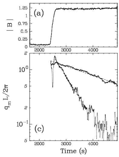
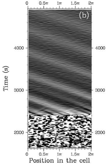
Figure 7: Apparition of modulated waves at hydrothermal wave onset produced by a fast increase of $\epsilon$ from a small negative value below onset to $\epsilon=0.16$ ($\Delta T=3.60$ K) near $t=2250$ s. (a): Mean amplitude $|B|(T)|$ of the carrier left-traveling wave showing the control parameter change. (b): Spatio-temporal diagram of the phase gradient $\partial_{X}\Phi$ of the left-traveling wave. (c): Temporal evolution of the wavenumber-modulation amplitude $q_{\rm m}(T)$ extracted from phase-gradient data (b) by Hilbert transform. The upper curve show the $K_{\rm M}=2\pi/L_{\rm p}$ fundamental mode of the modulation and the lower curve corresponds to the first spatial harmonic at $K_{\rm M}=2\cdot(2\pi/L_{\rm p})$. The dashed lines are fits of the exponential decays.

Let start with a description of an experiment from linearly stable flow at negative $\epsilon$. When crossing threshold, a wave-pattern appears. A transient regime with competing counter-propagating wave is generally observed. This transient leads to a single right- or left-traveling wave as $\epsilon$ is increased. Once the single wave orbits along the channel, we notice that it is always a modulated wave.

An example is presented in Fig. 7. The modulated hydrothermal wave appears near $t=2250$ s after $\epsilon$ has been rapidly increased from a small negative value to $\epsilon=0.16$ ($\Delta T=3.60$ K).

Fig. 7a presents the mean amplitude $|B(T)|$ of the left-traveling wave, i.e., the relevant order parameter for this transition. The right-traveling wave $A$ exists only during a few hundred seconds at the begining of the transient. The transient itself is presented in details in paper II (section LABEL:sec:sources): the amplitudes for both waves and the detail of the competition are illustrated on a spatio-temporal diagram (Fig. LABEL:fig:st_competition of II).

Fig. 7b presents the local wavenumber $\partial_{X}\Phi$ of the left-traveling dominant wave. The phase is not defined until the amplitude of the wave becomes finite. Then, the wavenumber sets up around the mean value $k=53(2\pi/L_{\rm p})$, i.e., close to $k_{c}$. This picture shows the local variations of the wavenumber, which propagate at the group velocity and decay with time. This characterizes a modulated wave (MW) decaying toward a uniform hydrothermal wave (UHW). The modulation wavenumber is $K_{\rm M}=2\pi/L_{\rm p}$, i.e., the smallest possible wavenumber in the cell. The modulation appears to be damped: using a second Hilbert transform applied on $\partial_{X}\Phi$ (Fig. 7b), one can extract the amplitude $q_{\rm m}(T)$ of the local wavenumber modulation:

$$\partial_{X}\Phi(X,T)=q_{\rm m}(T)\ \exp i(\Omega_{\rm M}T-K_{\rm M}X)+...$$ (12)

This modulation amplitude is presented in Fig. 7c. The $K_{\rm M}=2\pi/L_{\rm p}$ fundamental mode is exponentially damped with a long characteristic time $\tau_{\rm M}=2600$s. The first spatial harmonic at $K_{\rm M}=2\cdot(2\pi/L_{\rm p})$ can also be extracted: it decays 4 times faster, as expected from linear dynamics. Higher harmonics are negligeable.

Once the modulation has relaxed, and the UHW (uniform hydrothermal wave) regime is reached, one can produce new modulations very easily, for example by dropping a fluid droplet in the channel or simply by touching the free surface with the needle devoted to fluid thickness measurements. We also frequently observe very small spontaneous modulations, due to experimental noise, that travel along the cell for several hundred seconds. When $\epsilon$ is varied from a relaxed UHW state, another modulated wave is produced: the larger is the $\epsilon$ jump, the larger the initial modulation amplitude is. Using droplets, very strong modulations can be initiated: the wavenumber modulation can reach five percent of the mean wavenumber value [14]. The very low damping rate is the signature of the presence of a secondary bifurcation for slightly higher $\epsilon$: the higher $\epsilon$, the larger $\tau_{\rm M}$. For different $\epsilon$ we plot the damping rate $\sigma_{\rm M}=1/\tau_{\rm M}$ in Fig. 8. The modulation wavenumber is $K_{\rm M}=2\pi/L_{\rm p}$ —the lowest achievable in a finite periodic box [55]— whatever $\epsilon$; the modulation frequency $\Omega_{\rm M}$ varies slowly with $\epsilon$, and this is discussed below (section 2.1.4). We observe $\sigma_{\rm M}$ to decrease with $\epsilon$ and to approach zero for $\epsilon=\epsilon_{\rm E}\simeq 1$. At this point, the wave pattern is unstable with respect to the modulational Eckhaus instability.

We wish to emphasize that measurements close to $\epsilon_{\rm E}$ are very long and difficult to perform because the pattern can break quite spontaneously. This is the reason why the transition is not clearly visible in Fig. 8. We will show that the fragility of the pattern is due to the nature of modulated wave solutions (see discussion in section 4.3). It is also obviously related to the metastability of the UHW with respect to changes of their integer mean wavenumber $k$: when $\sigma_{\rm M}$ gets smaller, the pattern becomes less stable and small fluctuations or perturbations due to the presence of the operator may induce a pattern change.

The next section describes the modulated waves above $\epsilon_{\rm E}$ wich are even more fragile.

Figure 8: Temporal decay rate of low wavenumber modulations ($K_{\rm M}=2\pi/L_{\rm p}$) versus $\epsilon$. Those data are obtained for patterns of mean wavenumber close to $k_{\rm c}$, i.e., within $\pm 2\pi/L_{\rm p}$. For $\epsilon$ close to $\epsilon_{\rm E}\sim 1$, modulations do not decay anymore and Eckhaus instability takes place. Measurements close to $\epsilon_{\rm E}$ are very long and difficult to perform because the pattern can break quite spontaneously.

2.1.2 Stable modulated waves above Eckhaus onset

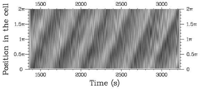
Figure 9: Space-time image of the local wavenumber of the $kL=55$ hydrothermal wave for $\Delta T=5.96$ K and $\epsilon=0.92$. This wavenumber modulation is non-linearly saturated and propagates steadily along time. According to Eq. 12 we measure: $q=(0.29\pm 0.05)2\pi/L_{\rm p}$. Spatial frequencies smaller than the third of the cell size are filtered.

Once $\epsilon$ is set greater than $\epsilon_{\rm E}$ we observe that the wavenumber modulation at $K_{\rm M}=2\pi/L_{\rm p}$ grows, then saturates and persists for several hours (Fig. 9). We have seen no evidence of hysteresis in this transition. It’s a supercritical Hopf bifurcation [14]. The bifurcated modulation amplitude is quite small compared to the modulation obtained either by changing the control parameter, either by forcing. Its amplitude is typically 5 times the noise level for the phase gradients in the best case for our standard experimental conditions at $h=1.7$ mm: the modulation can be detected on the phase gradients, but is too small to be measurable on the carrier wave amplitude. The amplitude of the wavenumber modulation represents typically $0.5\%$ of the mean wavenumber value.

Those modulated waves have been plotted on the stability diagram (Fig. 5). We notice that these stable modulated waves around $\epsilon_{\rm E}$ do not represent a well defined region in the $(\epsilon,k)$ diagram. They are observed in a very narrow band in $\epsilon$, the thickness of which is comparable to the noise level in this region. This noise level is very high due to the extreme sensitivity of modulated waves to noise and perturbations, which makes it very hard to reproduce exactly the experimental conditions. So, when the cell contains a supercritically saturated modulated wave pattern, the control parameter has to be changed by very small steps. Otherwise, the resulting perturbations produce strong modulations, break the pattern, and change its mean wavenumber. In this region of parameters, it is also impossible to measure the fluid thickness without perturbing and then breaking the pattern. We estimate the band of stable modulations to extend from $\epsilon_{\rm E}$ to $\epsilon_{\rm SN}$, $\epsilon_{\rm E}$ being typically close to unity around $k_{\rm c}$ and slowly decreasing with $k$, and $(\epsilon_{\rm E}-\epsilon_{\rm SN})$ is typically $0.2$ or $0.3$. The upper bound $\epsilon_{\rm SN}$ is named by reference to the saddle-node bifurcation of MAWs [36, 37] a point which will be emphasized in the discussion below (section 4).

Fragility seems thus to be the principal feature of those modulated patterns at $h=1.7$ mm and $k\sim k_{\rm c}$. Whereas plane- wave patterns may be strongly perturbed near the waves onset —$\epsilon\sim 0$, see Fig. 7—, the fragility to perturbations increases when $\epsilon_{\rm E}$ is approached, and becomes extreme in the supercritical Eckhaus band. The next paragraph describes how these modulated wave patterns spontaneously die above $\epsilon_{\rm SN}$.

2.1.3 Exploding modulated waves and spatio-temporal dislocations

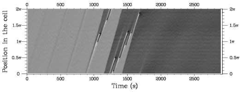
Figure 10: Transient evolution of a $k=55(2\pi/L_{\rm p})$ Eckhaus modulated wave pattern toward a stable $k=45(2\pi/L_{\rm p})$ UHW pattern, when $\epsilon$ grows from $0.92$ (pattern on Fig. 9) to $1.21$ above $\epsilon_{\rm SN}$. This image represents the local wavenumber without filtering or enhancement. At the first stage, the $K_{M}=2\pi/L_{\rm p}$ modulation travels at constant velocity. Its maximum peak value increases slowly (characteristic growth time $700$ s) while the amplitude of the fundamental ($2\pi/L_{\rm p}$) remains constant. Then, after $t=870$ s, both max amplitude and fundamental amplitude start growing on a faster scale ($\tau_{\rm M}=100$ s). Then, higher spatial frequencies start growing and generate ten successive traveling wavenumber peaks. The wavenumber peaks correspond to growing phase jumps: once they reach $\pi$, the local amplitude (not shown) simultaneously attaining zero and the local wavenumber changing sign, they create ten space-time defects which each annihilate one wavelength of the wave-pattern. The resulting $k=45(2\pi/L_{\rm p})$ pattern is Eckhaus stable: the remaining traces of modulations decay.

By increasing the constraint above this narrow stability band $(\epsilon>\epsilon_{\rm SN})$, we recover the usual Eckhaus behavior, illustrated in Fig. 10 which represents the evolution of a $k=55(2\pi/L_{\rm p})$ modulated carrier pattern when $\epsilon$ is increased above $\epsilon_{\rm SN}$. We observe the spontaneous growth of high wavenumber modulations leading to space-time defects or amplitude holes [8] where the amplitude goes to zero and the phase jumps by $\pi$ (see Fig. 10 and caption for details). After ten phase jumps, the mean wavenumber of the carrier TW has decreased to $k=45(2\pi/L_{\rm p})$ and the pattern relaxes towards a non-modulated UHW state. Note that this example corresponds to a strong increase of the control parameter $\epsilon$. For smaller steps above $\epsilon_{\rm SN}$, the transient state lasts much longer: many more traveling modulations are observed, whereas only five or six of them reach the zero-amplitude level and change the carrier pattern wavenumber. This recalls the slow chaotic state [4] for Eckhaus transition of subcritical TW. The non-saturated growth of waves-modulations have been described as the basic mechanism for the development of the Eckhaus instability in several systems [4, 6, 7, 9, 10] leading to spatio-temporal defects and subsequent variation of the mean wavenumber. The only difference in our system is the basic state which is already slightly modulated. This is quite invisible on the spatio-temporal diagrams (Fig. 10): the original traveling modulation is tiny and would need a strong contrast enhancement to appear on the picture. Notice also the wavenumber of the growing modulations which rapidly increases to typically $K_{\rm M}\sim 6$ to $8(2\pi/L_{\rm p})$ instead of $(2\pi/L_{\rm p})$. A very interesting observation has been made by Liu and Ecke [9] in rotating convection: the further the control parameter is increased into the unstable Eckhaus band, the more the pattern number of wavelengths is changed. Our system currently looses as much as six to ten wavelengths. This phenomenon is probably favored by the existence of the supercritical band: when defects appear, the distance to $\epsilon_{\rm E}$ is already finite. This effect depends probably also of the slopes of $\epsilon_{\rm E}(k)$ and $\epsilon_{\rm SN}(k)$.

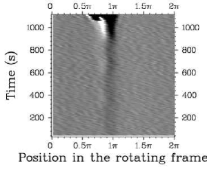
Figure 11: Same wavenumber data as in Fig. 10, presented in the frame rotating at the modulation velocity. From the spatio-temporal image, an averaged profile ($600\,{\rm s}<t<800\,{\rm s}$) of the modulation phase gradient is extracted.

Fig. 11 presents the growing modulation in the rotating frame where it is stationary. The shape of the profile does not vary very much until the first defect appears. Such profile is very similar to the typical phase-gradient profiles of MAWs [36].

Once the pattern has relaxed to a lower wavenumber, we may again increase $\epsilon$. Eckhaus modulations and pattern breaking occurs again, until the mean wavenumber reaches $44$ or $45(2\pi/L_{\rm p})$. However, below $49$ or $50(2\pi/L_{\rm p})$, the nature of the modulations changes dramatically as will be shown in section 2.2.

2.1.4 Velocity of modulated waves and group velocity

Figure 12: Velocity $v_{\rm G}=\Omega_{\rm M}/K_{\rm M}$ of small wavenumber ($K_{\rm M}=2\pi/L$) modulations vs. $\epsilon$. Circles ($\circ$) correspond to modulations decaying towards UHW. Plusses ($+$) correspond to stable or metastable (far before the apparition of space-time defects) modulations. These data are taken in the central wavenumber-band around $k_{\rm c}$, i.e., for $53\leq kL/2\pi\leq 57$.

The observation of traveling modulations of waves gives a basic information: the phase velocity of the modulation. As far as small smooth modulations can just be considered as perturbations of the wave envelope, their velocity is equivalent to the hydrothermal wave group velocity. This is the case for damped modulated waves below $\epsilon_{\rm E}$, at least just before they vanish. In fact the velocity is almost independent of the amplitude of the modulation. We extract this velocity from the study of the modulation frequency $\Omega_{\rm M}$, for wavenumbers in the very central band around $k_{\rm c}$, i.e., for $53\leq kL/2\pi\leq 57$. The group velocity $v_{\rm G}=\Omega_{\rm M}/K_{\rm M}$ is plotted on Fig. 12. Extrapolation at the wave onset is used to measure the value of $s$ given in Eq. 10. The variation of $\Omega_{\rm M}$ (or $v_{\rm G}$) with $\epsilon$ may also be used in the fit of the HOCGL coefficients, because it is one of the terms in the development of the eigenvalue $\sigma$ for the secondary instability mode:

$$\sigma=-D_{\parallel}K_{\rm M}^{2}+iv_{\rm G}K_{\rm M}+{\rm O}(K_{\rm M}^{3})$$ (13)

where $D_{\parallel}$ is the phase diffusion coefficient for modulational perturbations, directly related to the damping of the modulation amplitude (Fig. 8).

Fig. 12 also presents a few data concerning supercritical traveling modulations. Some values of $v_{\rm G}$ are a bit larger than what would be extrapolated from the damped modulations data. This may be the sign of a particular selection of the modulation velocity [36, 37] (see discussion in section 4).

A contrario, above $\epsilon_{\rm SN}$, we observe the modulation velocity to decrease at the end of the growth phase, just before the nucleation of spatio-temporal dislocations (Fig. 10): a smooth trace of each modulation keeps traveling at the group velocity until it disappears, while the sharp phase-gradient peaks slow down, in the laboratory frame, near the defects core (Fig. 13).

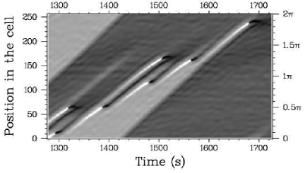
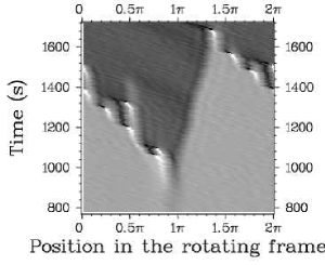
Figure 13: Same wavenumber data as in Fig. 10. (a) Time detail of the pattern around defect cores in the laboratory frame: please note how the hole cores slow down before disappearing. (b) Global view presented in a frame rotating at the initial modulation velocity. Using much lower contrast than in Fig. 11, one can follow the defects during their whole life: the hole core velocity is negative in this frame.

2.2 Large square modulated waves far from $k_{\rm c}$

Traveling wave patterns at low wavenumber $k\lesssim 45(2\pi/L_{\rm p})$, below the central band are also unstable with respect to Eckhaus instability, but in somewhat different conditions. Once the Eckhaus onset is crossed, very strong square modulations appear. The name square is chosen because the local wavenumber and frequency signals along space and time represent a square signal, or at least exhibit a sharp front. The amplitude of these signals saturates at a very high value compared to the previous supercritical case: once the modulation passes at a point, the local phase-gradient changes of typically 10 to 20 percents of its mean value (compare to $0.5\%$ in the previous case close to $k_{\rm c}$). The modulations appear spontaneously with a large amplitude: it is probably a subcritical bifurcation with a high order non-linear saturation, i.e., again a very different pattern from the classical subcritical Eckhaus transition [4]! Another feature of the square modulations is their spatial wavenumber $K_{\rm M}$ or spatial period $P=2\pi/K_{\rm M}$. We observed $P$ to vary from $L_{\rm p}$ to $L_{\rm p}/5$, instead of being uniformly $L_{\rm p}$ in the supercritical case. Fig. 14a present such $P=L_{\rm p}$ square pattern. The wavenumber profile and the amplitude profile along the channel are shown in Fig. 14b and Fig. 14c respectively.

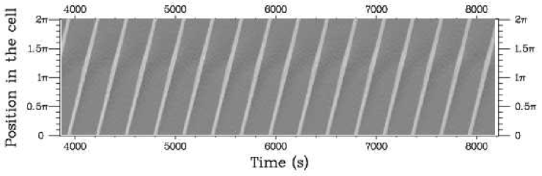
Figure 14: Strong square modulations for $\epsilon=1.32$ ($\Delta T=7.2$ K) and mean wavenumber $k=46(2\pi/L_{\rm p})$. The local and instantaneous wavenumber is displayed on the space-time diagram (a). This pattern may be compared to two imbedded regions of quasi-uniform wavenumber $k=44(2\pi/L_{\rm p})$ and $k=59(2\pi/L_{\rm p})$ traveling together. The spatial wavenumber profile (b) and wave-amplitude profile (c) are averaged in the rotating frame over eight periods.

Those square patterns are not systematically observed when the experiment is reproduced. Moreover, they may decay very slowly (typically over a day) and vanish. No systematic study has been realized over such time scale. If the control parameter is increased sufficiently, the sharp high wavenumber part of the signal generates spatio-temporal dislocations and the pattern looses $L_{\rm p}/P$ wavelengths. The nature and stability of square modulated waves is an open question.

2.3 Spatio-temporal chaos at high $\epsilon$ and far from $k_{\rm c}$: toward a globally restored symmetry

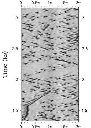
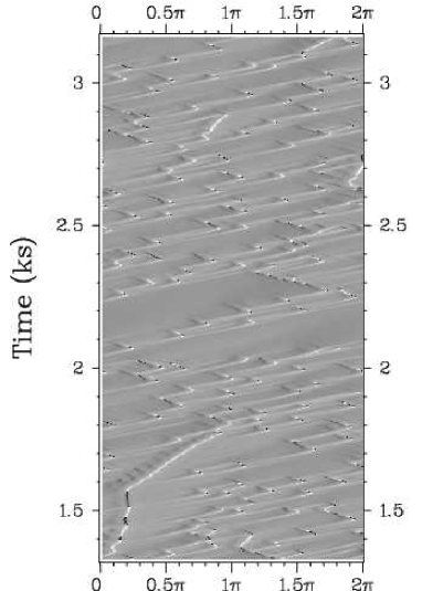
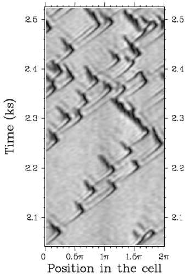
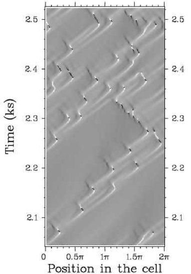
Figure 15: Spatio-temporal chaos due to small scale traveling holes and modulations. Spatio-temporal diagrams of the local and instantaneous amplitude $|A|$ (left) and of the local wavenumber (right) of the right-traveling wave for $\epsilon=3.11$. The gray scale for amplitude data is proportional to $|A|$: zero amplitude appears black. The mean wavenumber fluctuates around $k=43(2\pi/L_{\rm p})$. A general view is given (top). A region showing the most common holes patterns is enlarged (bottom). Some slower patterns on the general view correspond to couples of source and sink, traveling very close to each other and remaining parallel. Those objects cannot be studied without the left-traveling wave information. These diagrams are presented in the laboratory frame. We estimate the group velocity as being the velocity of small amplitude modulations far from the $A=0$ defects cores.

In the above sections, description of states have been made which —except for exploding modulations above $\epsilon_{\rm SN}$— presents only phase dynamics. As a consequence, the integer mean wavenumber $k$ was considered as a constant parameter in the dynamics. In this section, we will describe amplitude-chaotic patterns which are not concerned anymore by this constraint: the mean wavenumber may fluctuate since the presence of topological defects allow the phase to change by steps. This is an example of defect-chaos [30].

Once the wavenumber decreases below $43$ or $44(2\pi/L_{\rm p})$, no periodically modulated waves are ever observed. The $k=43(2\pi/L_{\rm p})$ UHW can be driven up to $\epsilon\sim 2.6$, i.e., very far from the onset of waves. For higher $\epsilon$ the system transits to disordered patterns instead of periodically modulated waves; then, the mean wavenumber of the pattern ceases to behave as a constant of the dynamics. Three different regimes may be encountered. They have been studied in the range $2.8\lesssim\epsilon\lesssim 3.9$. Those regimes need very long observations in order to be characterized: a very slow temporal intermittency regime is observed which makes those chaotic states appear and disappear, intercalated with metastable UHW in a very-low-wavenumber range ($39\lesssim kL_{\rm p}/2\pi\lesssim 43)$. The characteristic time of this intermittency is of order of 2-10 hours.

The first regime shows UHW being densely invaded by traveling holes (Fig. 15). These objects behave as localized modulated waves existing over much smaller scales than the low wavenumber modulations described above. They present a complex dynamics and interact together. They travel in the same direction as the carrier wave, but once they reach their minimal amplitude, very close to zero, the direction of propagation may reverse. Traces of the counter-propagating wave are sometimes observed in this backward traveling part of the hole. Mean wavenumbers are typically around $44(2\pi/L_{\rm p})$.

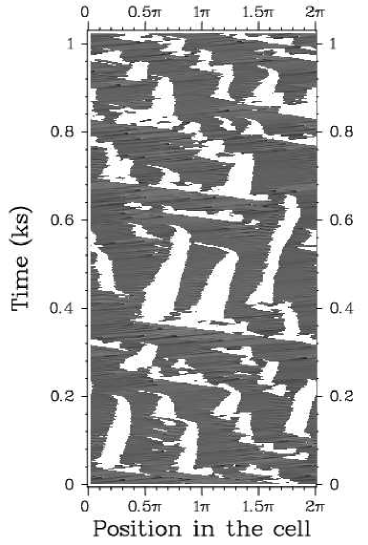
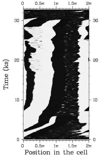
Figure 16: Spatio-temporal chaos due to sources and sinks dynamics, i.e., counter-propagating waves competition. This figure shows spatio-temporal diagrams of the local and instantaneous frequency of the wave-patterns after a Hilbert transform in space. Right (resp. left) traveling waves appears as dark (resp. light) areas. The left image ($\epsilon=3.25$ and $k\sim 43(2\pi/L_{\rm p})$) presents a dominant right-traveling wave with bubbles of left-traveling wave in a $3/4$–$1/4$ mean ratio. This ratio reverses several time during the complete data acquisition. The contrast is adjusted to show traveling modulations and holes in the dark right-traveling wave region, and white left-traveling regions are saturated. The right image ($\epsilon=2.84$ and $k\sim 46(2\pi/L_{\rm p})$) presents a symmetric pattern: right- and left-traveling wave in a $1/2$-$1/2$ mean ratio. Please note the length of the presented data set (9 hours) which reveals the temporal intermittency: the right-traveling wave dominates at the beginning and at the end.

The second regime contains right- and left-propagating waves domains in typically $1/4-3/4$ proportion (Fig. 16, left). The $x\mapsto-x$ symmetry, broken at the hydrothermal wave threshold is thus partly restored at a global level. The minor wave appears in small “bubbles” separated from the dominant waves by traveling sources and sinks. One can note that, during the main lifetime of the minor-wave-regions, the source velocity is selected while the sink dynamics is much more erratic until the source/sink pair collides and annihilates. Such sources/sinks wave patterns show a mean wavenumber just a bit larger (Fig. 5) than the one of traveling hole patterns presented above (Fig. 15). In fact, traveling holes and modulations still exist between sources and sinks. The source velocity is typically one order of magnitude smaller than the group velocity. Such sources/sinks dynamics looks very similar to the one reported in numerical simulations for small coupling coefficients by van Hecke, Storm and van Saarloos (Fig. 10 of Ref. [56]) and by Riecke and Kramer (Fig. 11 of Ref. [57]).

In the third situation (Fig. 16, right), the $x\mapsto-x$ symmetry appears to be totally restored at the global level: right- and left-propagating waves regions are equally represented. Thus we observe the sources to remain fixed along time, being only slightly affected by small erratic movements of the sinks. Observed patterns typically exhibit two right-traveling and two left-traveling domains along the cell (Fig. 16, right). The study of the source velocity selection with right- and left-traveling waves repartition is under progress and will be published elsewhere. When the sources and sinks remain at fixed locations, the annular system can be seen as equivalent to adjacent finite systems [56] of smaller sizes. The waves emitted by the sources are modulated waves, very similar to those reported in the finite box (section LABEL:sec:rect_seuil2 of II). Those modulations travel across the whole cell and even pass through the sinks —which are extended in space because $|A|$ and $|B|$ vary smoothly in their core. A complex dynamics can be observed.

Finally, we wish to emphasize the global restoring of the $x\mapsto-x$ symmetry in both regimes of mixed right- and left-traveling waves: while the wave-proportion fluctuates around its mean value, we often witness dominant wave direction reversal. Reversal time-scales are comparable to the temporal-intermittency time-scales described above. At such high control parameter, the fluctuation level is high and it is thus easy for the system to transit between symmetric states, as well as between different dynamical regimes.

3 Modulated traveling waves: high modulation amplitude solutions in thin layers

Some experiments have been performed in the annular channel with a smaller fluid depth, down to $0.8$ mm. The fluid height $h$ is the main length scale of the problem [27]. The wavelengths, $k_{\rm c}^{-1}$ and $\xi_{0}$ directly scale on $h$ and so non-dimensional channel length $L^{*}=L_{p}/\xi_{0}$ is increased. Then, assuming $\xi_{0}\propto h$, for $h=1.7$ mm, $h=1.2$ mm and $h=0.8$ mm, one respectively gets $L^{*}=98$, $L^{*}=140$ and $L^{*}=210$, i.e., very extended cells. As the transverse aspect ratio of the cell also increases when $h$ decreases, we may expect the occurence of 2-D effects [17, 18]. In practice, such effects may occur only below $h_{\rm c}=1.1$ mm and they are negligeable (a slight curvature of the wave front is observed for $h=0.8$ mm) for the patterns presented in this paper. Note however, that the smaller $h$ is, the more the system is sensitive to fluid evaporation.

We have illustrated in the previous section that the dynamics depends on the distance to $k_{\rm c}$, and we may suspect how variation of $k_{\rm c}$ as small as one unit of $2\pi/L_{\rm p}$ [58] may modify the dynamics, while the pattern wavenumber has to remains fixed to satisfy the periodic boundary conditions. For the smallest heights the uncontrolled variation of $h$ would probably be responsible of a continuous drift of the Eckhaus stability limit which would thus be periodically crossed by the system, this process inducing series of successive wavenumber transitions.

3.1 Modulations of large period at small $\epsilon$

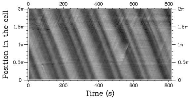
Figure 17: Strongly modulated wave at $h=0.80$ mm and $\epsilon=0.25$. Spatio-temporal diagram of the local wavenumber. This nonlinearly saturated modulation of a mean wavenumber $k=101(2\pi/L_{\rm p})$ traveling-wave is due to the occurence of the Eckhaus instability. The instability limit is crossed by varying $k-k_{\rm c}$ at constant $\epsilon$: a slow evaporation make $k_{\rm c}$ vary while $k$ is kept constant due to the cell periodicity.

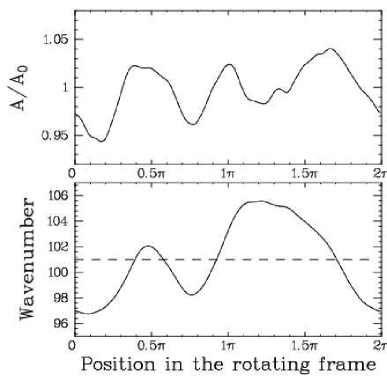
Figure 18: Amplitude (top) and wavenumber (bottom) profiles of the modulated wave presented in Fig. 17. The profiles are averaged along time in the rotating frame. The amplitude of the modulation is typically $\pm 5\%$ of the mean value $A_{0}$ of the amplitude and of the mean value $k=101(2\pi/L_{\rm p})$ of the wavenumber (dashed line).

The following data have been recorded during a long experiment at constant $\Delta T=4.80$ K and letting $h$ naturally decrease at a rate of $0.021$ mm/day. The data presented in Fig. 17 are recorded at $h=0.80$ mm, i.e., shortly before crossing the frontier between hydrothermal waves and basic flow (see Fig. 3). In this region, the slope of the frontier is large and $\epsilon$ is not precisely known but can we can estimated it to be roughly $0.25$ ($\Delta T_{\rm c}\simeq 3.9$ K). This experiment presents thus the classical Eckhaus transition, i.e., the crossing of the Eckhaus boundary at small and decreasing $\epsilon$. Fig. 17 shows the spatio-temporal diagram of the local-wavenumber for a strongly modulated pattern. The carrier wave has 101 wavelengths in the cell while the wavenumber of the modulation $K_{\rm M}=2\pi/L_{\rm p}$ is low or its period $P=L_{\rm p}$ is large. This pattern is saturated by non-linearities, because all quantities are constant along time. As far as the amplitude of the modulation is large on all fields, we tried to determine the group velocity and some CGL coefficients from the frequency-wavenumber and amplitude-wavenumber relation extracted from local values over the whole data set [43, 34]. We thus get:

$$k_{\rm c}=1.28\,{\rm mm}^{-1}=102.25\,(2\pi/L_{\rm p})$$

$$\xi_{0}=3\,{\rm mm}$$

$$v_{G}=\partial\omega/\partial k=1.61\,{\rm mm.s}^{-1}$$

Let us emphasize here that this method is impossible to apply to the $h=1.7$ mm modulated wave because the modulation amplitude is too tiny.

We also extracted the spatial profiles for the amplitude and phase-gradients (Fig. 18). These profiles show the fine structure of the modulation which is rich in harmonics.

3.2 Modulations of small period

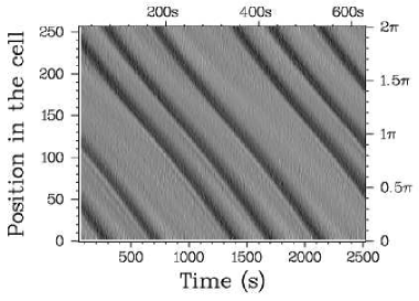
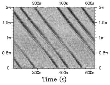
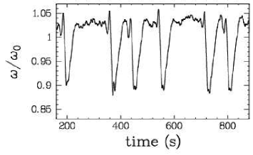
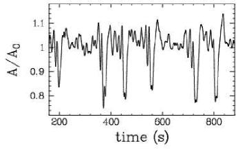
Figure 19: Modulated wave pattern at $h=1.2$ mm and $\Delta T=4.8$ K ($\epsilon\simeq 0.5$). Spatio-temporal diagram and time-serie of the local frequency are displayed on the left. Spatio-temporal diagram and time-serie of the local wave-amplitude are displayed on the right. The maximum local variations are of order of $0.2$ relatively to the mean values $\omega_{0}$ and $A_{0}$. The small oscillations of the modulations velocity is probably due to a rough adjustment of the channel horizontality which induces a height modulation.

In another experiment, the fluid height is set to $1.2$ mm and the temperature difference is increased from the onset value to $\Delta T=4.8$ K ($\epsilon\simeq 0.5$). Strongly modulated waves are also observed. Three modulations travel along the cell (Fig. 19). These modulations have a small spatial period $P\simeq L/3$ and cannot be described with a simple Fourier model as Eq. 12. The three modulations look like solitary waves.

3.3 Turbulent modulated wave far from threshold

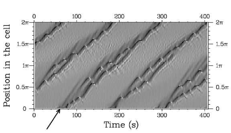
Figure 20: For $h=1.5$ mm and $\Delta T=15.4$K ($\epsilon=4$), two turbulent modulations are observed to travel in parallel along the channel. This diagram presents the local wave-frequency. The traveling modulations produce series of spatio-temporal defects. We may observe three characteristic velocities: (i) the mean velocity of the global turbulent pattern, (ii) the velocities of the sharp black or white peaks corresponding to traveling holes and (iii) the velocity of small smooth and damped holes or modulations leaving the main pattern, identified by the arrow, and assumed to represent the effective group velocity. The mean wavenumber is $k=41(2\pi/L_{\rm p})$ and we note that most holes are dark, i.e., correspond to negative wavenumber peaks.

Another type of traveling modulated waves (Fig. 20) has been observed for $h=1.5$ mm and $\Delta T=15.4$ K ($\epsilon=4$). This pattern of period $P=L/2$ is a turbulent modulation: the wave amplitude is strongly modulated and often reaches zero in the core of spatio-temporal defects. These defects occur in the trace of sharp traveling holes (black or white peaks of frequency on the figure). The wavenumber is not defined anymore in these spatio-temporal dislocations. This is an example of defect-mediated turbulence [59, 60] or defect-chaos [30, 61, 36]. One should note that the typical distance between defects is of order of $L/10$ ($50$ mm) to $L/2$ ($250$ mm), whereas the correlation length $\xi=\epsilon^{-1/2}\xi_{0}$ is of order of $3$ mm, even smaller than the wavelength $L/41$ ($12$ mm).

An interesting observation concerns the local velocity of various localized patterns of the phase-gradient field: the strongest modulations, i.e., the high peaks of phase-gradients travel more slowly than smoother phase modulations. Furthermore, all the smooth modulations are damped and propagate at the same speed, which we identified as the effective group velocity, represented by an arrow on Fig. 20. This is a general observation for all data in the annular channel: localized peaks of phase-gradient (close to space-time dislocations, for example) travel in the laboratory frame at slower velocity than the group velocity, i.e., at a negative velocity in the comoving frame of the wave pattern, the frame which is used for theoretical and numerical study of single wave patterns.

4 Modulated waves in a periodic channel: discussion

4.1 The context of modulated waves

We have presented an overview of the known dynamics of modulated waves in our long annular channel. Modulated waves appear to be everywhere: near hydrothermal waves onset as well as for high control parameter values, near the critical wavenumber value as well as far in the side band.

Modulated waves concern mainly single traveling waves, the situation of most patterns in this paper, but seem to be relevant in competing-wave patterns as well (Fig. 16). Other forms of modulated waves in bounded boxes are presented in section LABEL:sec:rect_seuil2 of the companion paper II.

Theoretical study of disordered pattern was mostly initiated on single 1D and 2D Complex Ginzburg-Landau models [30, 61, 62]. These first studies where only concerned by zero mean phase-gradient solutions ($\nu=0$) in periodic boundary conditions, i.e., solutions at $k=k_{\rm c}$. The mean-phase gradient, equivalent to our mean wavenumber, and also called winding number is usually defined as:

$$\nu\equiv\frac{1}{2\pi}\int_{0}^{L}\partial_{X}\Phi dX$$ (14)

Those works have evidenced the transition from phase- to defect-chaos in the case of Benjamin-Feir (BF) unstable regimes, and generally ignored the Eckhaus instability which is unknown at zero mean phase-gradient unless higher order terms are considered as in section 1.5. Our experiment, however, shows supercritical Eckhaus instability regimes for small mean phase gradients $\nu\simeq 0$. Furthermore, a striking feature is the overlap of the region of supercritical Eckhaus or Benjamin-Feir instabilities [7] with the region of phase chaos at $\nu=0$ [30]. Both type of solutions correspond to solutions that may be described by the phase equation —they may be called phase-solutions—, and they occur in the same region of the CGL parameter-space, near the BF border line.

The case of non-zero $\nu$ was pointed out by Montagne et al. [63] and Torcini et al. [31] on the basis of numerical simulations. Recently, this problem has been extensively studied by numerical analysis based on an equivalent ODE system [35]. Both $\nu=0$ and $\nu\neq 0$ cases have been treated by Brusch and his collaborators in Refs. [36] and [37] respectively.

Major contributions to the competing ($\lambda>1$) or cooperating ($\lambda\leq 1$) two-waves problem have been made respectively by van Hecke et al. [56] and Riecke and Kramer [57]. $\lambda$ is the real part of the coupling coefficient of CGL Eq. 2.

Finally, other authors have studied the bounded box case [64], corresponding to the experiments described in II for a single wave, and the semi-infinite case [65].

4.2 Modulated Amplitude Waves — MAWs

Modulated wave patterns have been especially recognized by Brusch and collaborators [35, 36, 37] who proposed the name Modulated Amplitude Wave or MAW, for those solutions of single CGL equation. All modulated waves described in this section can be viewed as MAWs. We did not use this vocabulary in the previous sections in order to avoid possible confusions about both amplitude and modulated waves terms. In modulated amplitude wave, amplitude refers to complex amplitude in CGL, but in experimental data, the amplitude refers generally to the modulus of the complex field. In other word, when discussing above on modulated waves (MW), we mean the modulations and the carrier wave whereas theoretical MAWs describe the modulation alone, ignoring the carrier wave. Finally, the group velocity of MAWs corresponds to the velocity selection of each particular MAW, while the CGL group velocity $s$ is eliminated by referential change. However, in the experimental frame the modulation velocity is, at first order, $s$ (with some HOCGL corrections), and the specific MAW velocity could be only a small correction to be extracted from experimental noise. All those reasons justify the language used in the above sections. Anyway, in this discussion, observational results and MAWs properties will be directly compared using MAWs language in order to ease the comparison of experimental results with theoretical papers.

MAWs numerical study is based on few parameters: the CGL coefficients $c_{1}$ and $c_{2}$, the mean phase-gradient $\nu$, the spatial period $P$ of the MAW solutions and the size of the box $L$. $P$ and $L$ have been identically defined above, $\nu$ represents the mean reduced wavenumber $q=\xi_{0}(k-k_{\rm c})$ and, as discussed in section 1.5, our HOCGL coefficients together with $\epsilon$ play a similar role than CGL $c_{1}$ and $c_{2}$ in parametrizing the problem. Brusch et al. generally keep one of the $c_{i}$ constant (e.g., $c_{1}=3.5$ in Ref. [37]) and vary the other coefficient to explore the dynamical regimes and instabilities. This changes the properties of the system with respect to the Eckhaus/Benjamin-Feir transition and the $L_{1}$ and $L_{3}$ lines. Experimentally, we encountered similar transitions by simply varying $\epsilon$ which, because of the existence of HOT, also changes the distance of the system to Eckhaus and BF transition (section 1.3). On the qualitative point of view, our exploration of the parameter space is of the same nature.

Let’s recall some of the main results of MAWs study. Different types of MAW solutions have been observed: homoclinic orbits corresponding to infinite $P$ patterns and heteroclinic orbits corresponding to finite $P$ patterns. Coherent MAW patterns have been shown to appear through a forward Hopf bifurcation (HB) and loss their stability through a saddle-node bifurcation (SN). Therefore, the stable MAW branch is surrounded by an unstable branch, both connecting at the saddle-node. Different stable MAW branches may select various group velocity, a negative velocity branch, a zero velocity branch and a positive velocity branch through a drift pitchfork bifurcation. Finite size effect have been shown to be of major importance: transitions may be parametrized by CGL coefficients as well as by $P$ [36] and the existence and the stability of a $P$-period solution strongly depends on the relative value of $P$ and the box size $L$. Unstable MAWs have been shown to be the seeds of spatio-temporal defects leading either to pattern breaks (in the Eckhaus unstable case) or to defect chaos. In phase chaos regimes, local fluctuations of the phase-gradient or amplitude can be viewed as single MAWs in interactions.

4.3 Supercritical Eckhaus modulated wave patterns near $k_{\rm c}$

It is now well known that supercritical modulations of traveling waves may result from a supercritical Eckhaus transition [54, 7, 14, 66, 37]. Since Eckhaus instability is a low-wavenumber instability, we discussed this behavior over the amplitude of the first mode $K_{\rm M}=2\pi/L$ [14]. However, it is clear (Figs 7, 9 and 10. See also Fig. 3 of Ref. [14]) that finite spatial harmonics contribute to the modulation profile. This shape (Fig. 11) is qualitatively in very good agreement with the calculated shape of theoretical MAW solutions. Supercritical Eckhaus modulations are to be searched among $P=L$ stable MAWs [37].

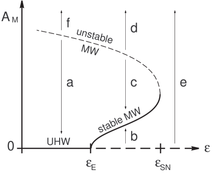
Figure 21: Schematics of the dynamics of experimental modulations. The control parameter $\epsilon$ is varied in abscissa and a characteristic instantaneous measure of the modulation amplitude $A_{\rm M}$ (e.g., amplitude $|A|$ or phase-gradient variation amplitude) is plotted in ordinate. Several typical paths (a-f) have been traced. See section 4.3 for explanations and discussion.

Moreover, the temporal dynamic of the experimental modulated wave solutions is very well illustrated in Fig. 13 of Ref. [37] (on page XXX of the present volume) which presents some spatio-temporal diagram exhibiting exploding, relaxing and non-linearly saturating MAWs. Fig. 21 supports an overview of the experimentally observed modulation regimes inspired by Brusch et al.’s presentation. Typical experimental path have been schematized. The main difference stays in the way a state is prepared: as explained above, initial modulations are produced by simply changing $\epsilon$ (section 2.1.1), so the zero modulation initial condition is, in practice, unreachable. The dynamics will strongly depend on an initial hardly controlled condition. Path (a) is the most common experiment below $\epsilon_{\rm E}$ (Fig. 7), whereas path (f) illustrates the fragility of Eckhaus stable waves (section 2.1.2) and has been the source of strong questioning about the experiment reproducibility at its beginning! Path (c) is the usual way for stable modulated patterns to appear because of the initial amplitude. So path (b) as never been observed and would probably require a very slow increase of the control parameter to be produced experimentally. Path (d) is what happens when the control parameter is increased too much from an initial stable modulated pattern. Finally, path (e) describes the destabilization of the pattern (Fig. 10) above $\epsilon_{\rm SN}$. Brusch et al. noted that such path, passing close to the saddle-node, seems to saturate as a stable MAW for a long time before leaving the SN region. This behavior is clearly observed in the experiment. For example, the stable modulation in Fig. 9 is obtained after a long decrease of an initial modulation as on path (c). Then, at the end of the acquisition, $\epsilon$ is increased a little. We then observe a quasi-stable MAW on the first part of Fig. 10. This MAW has a constant amplitude for its first spatial Fourier mode, but the maximal value of the phase-gradient slowly increases with time up to $t=870$ s: the modulation gets sharper and sharper. For $t>870$ s, all Fourier modes, even the fundamental, start exponentially growing with a short characteristic time up to the birth of the first spatio-temporal defect.

From a Fourier-modes point of view, Eckhaus instability appears once the highest unstable wavenumber becomes larger than $2\pi/L$. Suppose this mode is saturated by the non-linearities. If the control parameter increases, the spatial harmonics $2n\pi/L$ also becomes unstable. If higher harmonics are less saturated than the fundamental mode and the lower harmonics are, the modulated pattern will become unstable above a second critical control parameter: the stable-modulation domain is bounded from above. Such basic Fourier mode description may be explored experimentally. One can clearly see how, far from $\epsilon_{\rm E}$ as on Fig. 7, the harmonics decay much faster than the fundamental. The decay rate ratio between fundamental and first harmonic is 4.1, close to 4, i.e., proportional to $K_{\rm M}^{2}$. Upper harmonics remains within the noise level. This effect is in agreement with the classical low-wavenumber limit of the Eckhaus instability (Eq. 13). On the other hand, close to $\epsilon_{\rm E}$, such comparison seems to fails. Further study would be needed to bring quantitative conclusions.

The high degree of similarity between experimental and numerical realizations allows us to conclude that both experimental modulated waves and stable MAWs are the actual solutions of supercritical Eckhaus unstable patterns in periodic boundary conditions traveling-wave systems. As this does not seem to depend on the exact Ginzburg-Landau model, it is probably a general property of the Eckhaus modulational instability regardless of the nature of the wave system.

Janiaud et al. [7] have calculated the region where Eckhaus instability is supercritical in the $(c_{1},c_{2})$ plane. This region appears to border the BF line $1+c_{1}c_{2}=0$. We did not calculate this domain for the HOCGL equation but we noticed that the $\epsilon_{\rm E}(k)$ curve is quite horizontal (i.e., independent of $k$) in the central region of the stability diagram (Fig. 5). The parallel is easy to make: Eckhaus instability becomes Benjamin-Feir instability when all wavenumber are unstable. So we may imagine a CGL system varying coefficients $c_{1}(\epsilon)$ and $c_{2}(\epsilon)$ such that $1+c_{1}c_{2}$ decreases from positive value to zero at a given $\epsilon_{\rm E}$. This will close the Eckhaus stable domain from the top with an horizontal tangent at $k_{\rm c}$. This may be the reason for Eckhaus to be supercritical in this central band of wavenumber. Otherwise, Brusch et al. [37] also observed the stable MAWs to take place in the central wavenumber band close to $k_{\rm c}$. Phase-chaos patterns, which are another type of phase solutions, are also localized in this central band. More generally, we may propose that phase-solutions develop on a durable way only in domains of the parameter-space that are close to the Benjamin-Feir instability limit and for $k$ close to $k_{\rm c}$.

4.4 Low wavenumber patterns far from $k_{\rm c}$

On the other hand, defect-chaos and subcritical Eckhaus instability are numerically observed for large mean phase-gradients. Both patterns are characterized by the presence of defects and are to be studied considering both phase and amplitude variations [67]. For lower wavenumbers in our experiment, the Eckhaus border line becomes strongly dependent on $k$. The instability is probably subcritical although this has not been carefully investigated (section 2.2). Strongly “square”-modulated patterns (Fig. 14) and UHW are observed at the same region in the stability diagram (Fig. 5) for $k=45(2\pi/L_{\rm p})$ and $k=46(2\pi/L_{\rm p})$. This may account for subcritical bistability. The stability of patterns with wavenumbers outside the central band has also been investigated with the rectangular channel: the modulational instability has been carefully investigated for wavenumbers above $k_{\rm c}$ and is believed to be subcritical at convective threshold as well as at absolute threshold (section LABEL:sec:rect_seuil2 and Fig. LABEL:fig:ballon:ann&rect of II).

4.5 Defect chaos patterns far from $k_{\rm c}$

For the lowest studied values of $k$ —the biggest mean phase-gradient $|q|$ or $|\nu|$—, spatio-temporal defect chaos is observed (section 2.3, Figs 15 and 16). Also, defect chaos is numerically observed far from the BF line [30, 36], and interesting regions of simultaneous MAWs and defects are observed for large $\nu$. Do Fig. 15 data correspond to this region? This question cannot be answered owing to our present knowledge.

Another possibility is the occurrence of short-wavelength modulational instability [49, 29], which may perhaps describe better the pattern: when the intermittency changes a chaotic state into a single wave pattern, we again notice this pattern to be modulated at $K_{\rm M}=2\pi/L_{\rm p}$ with a fast decaying modulation. Thus, metastable UHW at very low $k$ in the intermittent region seems to be stable with respect to long-wavelength modulational instability, i.e., the classical Eckhaus instability. Chaotic regimes may thus be due to short-wavelength instability. A simple way to produce such instability in our HOCGL model Eq. (9) is to add a second fifth order term: $|A|^{2}A_{XX}$ with a small negative coefficient which will produce a negative diffusion coefficient for any $k$ at high wave-amplitude.

The above hypothesis are all based on a single equation model, and may eventually partly describe the first regime —a single wave with traveling modulations and holes (Fig. 15)— but is basically insufficient to describe source/sink patterns (Fig. 16, left). Comparable regimes have been observed numerically by Riecke and Kramer [57] in the case of small coupling coefficients $\lambda$. Our estimate for $\lambda=1.36\pm 0.2$ (section 1.6) is close to the region where chaotic competition is shown to occur: the “domain chaos” region takes place between the traveling-wave stability region for $\lambda>\lambda_{\rm r}$ and the standing-wave stability region for $\lambda<1$. For a given set of CGL coefficients, $\lambda_{\rm r}$ is found to be $1.3$ [57]. The “domain chaos” resembles our observations of non-symmetrical wave-competition.

On the other hand, the competing patterns with equivalent ratio of right- and left-traveling waves (Fig. 16, right) may be directly compared to modulated patterns in the bounded cell described in II: once source and sink select a zero velocity, they play quite the same role as boundaries in the rectangular channel [56], and the pattern may be viewed as several adjacent bounded patterns.

Finally, the turbulent traveling modulated pattern (Fig. 20) is an example of defect-chaos pattern involving a single traveling wave at first order (small counter-propagating wave patches develop around the defect-cores).

4.6 Modulation velocities

A question remains open: what does the modulation velocity represent? In many case through the paper, we supposed the modulation velocity to be equivalent to the group velocity. This is true for smooth modulation, e.g., for the lowest wavenumber mode at $K_{\rm M}=2\pi/L_{\rm p}$. So this proposition is valid for modulation as on Fig. 7. This leads to a precise determination of CGL group velocity $s$ (Eq. 10) by extrapolation at $\epsilon=0$ for $k\simeq k_{\rm c}$. This value agrees with the value measured in the rectangular cell (Fig. LABEL:fig:rec:velocity of II).

In the Eckhaus stable band near $k_{\rm c}$, the modulation velocity varies linearly (Fig. 12) as may be predicted by HOCGL equation (Eq. 9). In this frame, we recover Brusch et al.’s result: for $\nu=0$, the velocity of MAWs is zero below a drift pitchfork bifurcation occurring above the Hopf bifurcation to stable MAWs [36, 37]. The drift-pitchfork bifurcation has thus probably be crossed above $\epsilon_{\rm E}$ since the last points in Fig. 12 show a slightly higher velocity. Anyway, those measurements are noisy since the drift velocity is typically a tenth of the group velocity.

Low-$k$ UHW or modulated wave patterns far from $k_{\rm c}$ show a lower velocity with a similar $\epsilon$-dependence. The reduction of the velocity may be due to the unfolding of the drift-pitchfork bifurcation for $\nu\neq 0$ [37].

Traveling modulations leading to holes and defects (Figs 15 and 16) as well as traveling turbulent modulations (Fig. 20) exhibit velocity selection close to defects: the selected velocity is smaller (i.e., negative in the rotating frame) than the group velocity and eventually becomes negative (in the laboratory frame). The velocity varies very fast near the defect-core. Is this huge effect due to the presence of counter-propagating waves, or is it due to the proximity of a defect core?

Conclusion

Owing to their apparition via a supercritical instability with finite frequency, finite wavenumber and finite group velocity, hydrothermal waves were shown to be very well modeled by an amplitude equation of the complex Ginzburg-Landau type. Our one-dimensional hydrothermal-wave system can be considered as an experimental realization of a one-dimensional system of coupled CGL amplitude equations.

Concerning the amplitude equation itself, we obtained experimental evidence that higher-order terms should be included. Those terms probably play an important role for higher values of the control parameter, but can be discarded close to the onset of the instability.

In periodic boundary conditions, the Eckhaus secondary instability is supercritical for wavenumbers close to the critical wavenumber $k_{\rm c}$, whereas it is rather subcritical far from $k_{\rm c}$. This is confirmed by observations in non-periodical boundary conditions which spontaneously selects wavenumbers far from $k_{\rm c}$ and where the modulational instability is subcritical (paper II).

The development of the secondary Eckhaus modulational instability leads to the creation of various modulated traveling-wave patterns which have been presented, illustrated and discussed in the framework of modulated amplitude waves (MAWs), i.e., numerical solutions of the Eckhaus/Benjamin-Feir unstable CGL equation. The periodic boundary conditions imposed by the annular geometry favor the emergence of stable phase solutions, i.e., traveling modulations whose amplitude is stabilized by non-linearities. The amplitude of the phase-gradient modulation has a very large range: from less than a percent to typically ten percent of the mean phase-gradient of the carrier wave.

Several examples of defect-chaos have been reported. Eckhaus unstable patterns nucleate such defects once non-linearly saturated phase-modulated solutions become unstable. This occurs either because the control parameter is driven outside the stability domain or because finite amplitude perturbations break the patterns. Phase patterns have been shown to be very sensitive and fragile. This fact is by itself a result of our study and a challenge for experimental work. A major result provided by the study of MAWs dynamics [37] is the fundamental explanation of this fragility: owing to the presence of a saddle-node bifurcation and thus of an unstable branch over each stable phase branch, finite perturbations may generate growing phase-gradients leading to amplitude holes and the breaking of fragile modulated-wave solutions.

Finally, permanent regimes of defect-chaos have been studied. In most case they involve both competing right- and left-traveling waves and appear more complex than the extensively-studied defect-chaos domains observed for a single complex Ginzburg-Landau model equation. Though we constructed a higher-order CGL model in order to account for the reinforcement of the ($x\mapsto-x$) reflection symmetry breaking for high-amplitude single traveling-wave, we emphasized the restoring —at a global level— of the reflection symmetry in chaotic patterns of competing right- and left-traveling waves.

References

- [1] N. Garnier, A. Chiffaudel, and F. Daviaud. Nonlinear dynamics of waves and modulated waves in 1D thermocapillary flows. II: Convective/absolute transitions. Companion paper, part 2, 2002.
- [2] F. Daviaud, M. Bonetti, and M. Dubois. Transition to turbulence via spatiotemporal intermittency in one-dimensional Rayleigh-Bénard convection. Phys. Rev. A, 42:3388, 1990.
- [3] M. Rabaud, S. Michalland, and Y. Couder. Dynamical regimes of directional viscous fingering: Spatiotemporal chaos and wave propagation. Phys. Rev. Lett., 64:184, 1990.
- [4] P. Kolodner. Extended states of nonlinear traveling-wave convection. I. The Eckhaus instability. Phys. Rev. A, 46:6431, 1992.
- [5] P. Kolodner. Extended states of non-linear traveling-wave convection. II. Fronts and spatiotemporal defects. Phys. Rev. A, 46:6452, 1992.
- [6] G.W. Baxter, K.D. Eaton, and C.M. Surko. Eckhaus instability for traveling waves. Phys.Rev. A, 46:R1735, 1992.
- [7] B. Janiaud, A. Pumir, D. Bensimon, V. Croquette, H. Richter, and L. Kramer. Eckhaus instability for traveling waves. Physica D, 55:269, 1992.
- [8] J. Lega, B. Janiaud, S. Jucquois, and V. Croquette. Localized phase jumps in wave trains. Phys. Rev. A, 45:5596, 1992.
- [9] Y. Liu and R.E. Ecke. Nonlinear traveling waves in rotating Rayleigh-Bénard convection: Stability boundaries and phase diffusion. Phys. Rev. E, 59:4091, 1999.
- [10] T. Leweke and M. Provansal. The flow behind rings: bluff body wakes without end effects. J. Fluid Mech., 288:265, 1995.
- [11] P. Bot, O. Cadot, and I. Mutabazi. Secondary instability mode of a roll pattern and transition to spatiotemporal chaos in the Taylor-Dean system. Phys. Rev. E, 58:3089, 1998.
- [12] P. Bot and I. Mutabazi. Dynamics of spatio-temporal defects in the Taylor-Dean system. Eur. Phys. J. B, 13:141, 2000.
- [13] F. Daviaud and J.M. Vince. Traveling waves in a fluid layer subjected to a horizontal temperature gradient. Phys. Rev. E, 48:4432, 1993.
- [14] N. Mukolobwiez, A. Chiffaudel, and F. Daviaud. Supercritical Eckhaus instability for surface-tension-driven hydrothermal waves. Phys. Rev. Lett., 80:4661, 1998.
- [15] N. Garnier and A. Chiffaudel. Nonlinear transition to a global mode for traveling-wave instability in a finite box. Phys. Rev. Lett., 86:75, 2001.
- [16] N. Garnier and A. Chiffaudel. Convective and absolute Eckhaus instability leading to modulated waves in a finite box. Phys. Rev. Lett., 88:134501, 2002.
- [17] N. Garnier and A. Chiffaudel. Two dimensional hydrothermal waves in an extended cylindrical vessel. Eur. Phys. J. B, 19:87, 2001.
- [18] J. Burguete, N. Mukolobwiez, F. Daviaud, N. Garnier, and A. Chiffaudel. Buoyant-thermocapillary instabilities in extended liquid layers subjected to a horizontal temperature gradient. Phys. Fluids, 13:2773, 2001.
- [19] J.M. Vince and M. Dubois. Hot wire below the free surface of a liquid: structural and dynamical properties of a secondary instability. Europhys. Lett., 20:505, 1992.
- [20] J.M. Vince and M. Dubois. Critical properties of convective waves in a one-dimensional system. Physica D, 102:93, 1997.
- [21] R. Alvarez, M. van Hecke, and W. van Saarloos. Sources and sinks separating domains of left- and right-traveling waves: experiment versus amplitude equation. Phys. Rev. E, 56:R1306, 1997.
- [22] L. Pastur, M. T. Westra, and W. van De Water. Sources and sinks in 1D travelling waves. Submitted for this issue of Physica D., 2002.
- [23] M.K. Smith and S.H. Davis. Instabilities of dynamic thermocapillary liquid layers. Part 1. Convective instabilities. J. Fluid Mech., 132:119, 1983.
- [24] R.J. Riley and G.P. Neitzel. Instability of thermocapillary-buoyancy convection in shallow layers. Part 1. Characterization of steady and oscillatory instabilities. J. Fluid Mech., 359:143, 1998.
- [25] M.A. Pelacho and J. Burguete. Temperature oscillations of hydrothermal waves in thermocapillary-buoyancy convection. Phys. Rev. E, 59:835, 1999.
- [26] D. Schwabe, U. Möller, J. Schneider, and A. Scharmann. Instabilities of shallow dynamic themocapillary liquid layers. Phys. Fluids, 4:2368, 1992.
- [27] N. Garnier. Ondes non-linéaires à une et deux dimensions dans une mince couche de fluide. PhD. thesis, University Paris 7 Denis Diderot, 2000.
- [28] M.C. Cross and P.C. Hohenberg. Pattern formation outside of equilibrium. Rev. Mod. Phys., 65:851, 1993.
- [29] I. Aranson and L. Kramer. The world of the complex Ginzburg-Landau equation. Rev. Mod. Phys., 74:99, 2002.
- [30] B.I. Shraiman, A. Pumir, W. van Saarloos, P.C. Hohenberg, H. Chaté, and M. Holen. Spatiotemporal chaos ine the one-dimensional complex Ginzburg-Landau equation. Physica D, 57:241, 1992.
- [31] A. Torcini, H. Frauenkron, and P. Grassberger. Studies of phase turbulence in the one-dimensional complex Ginzburg-Landau equation. Phys. Rev. E, 55:5073, 1997.
- [32] N. Bekki and K. Nozaki. Formations of spatial patterns and holes in the generalized Ginzburg-Landau equation. Phys. Lett., 110A:133, 1985.
- [33] M. van Hecke. Building blocks of spatiotemporal intermittency. Phys. Rev. Lett., 80:1896, 1998.
- [34] J. Burguete, H. Chaté, F. Daviaud, and N. Mukolobwiez. Hydrothermal wave amplitude holes in a lateral heating convection experiment. Phys. Rev. Lett., 82:3252, 1999.
- [35] L. Brusch, M.G. Zimmermann, M. van Hecke, M. Bär, and A. Torcini. Modulated amplitude waves and the transition from phase to defect chaos. Phys. Rev. Lett., 85:86, 2000.
- [36] L. Brusch, A. Torcini, M. van Hecke, M.G. Zimmermann, and M. Bär. Modulated amplitude waves and defect formation in the one-dimensional Ginzburg-Landau equation. Physica D, 160:127, 2001.
- [37] L. Brusch, A. Torcini, and M. Bär. Nonlinear analysis of the Eckhaus instability modulated amplitude waves and phase chaos with non-zero average phase gradient. Submitted for this issue of Physica D, 2002.
- [38] G.S. Settles. Schlieren and shadowgraph techniques. Springer, 2001.
- [39] F. Mayinger and O. Feldmann. Optical measurements, techniques and applications, 2nd edition. Springer, 2001.
- [40] J.F. Mercier and C. Normand. Buoyant-thermocapillary instabilities of differentially heated liquid layers. Phys. Fluids, 8:1433, 1996.
- [41] D. Schwabe, U. Möller, J. Schneider, and A. Scharmann. Instabilities of shallow thermocapillary liquid layers. Phys. Fluids A, 4:2368, 1992.
- [42] M.A. Pelacho, A. Garcimartín, and J. Burguete. Local Marangoni number at the onset of hydrothermal waves. Phys. Rev. E, 62:477, 2000.
- [43] V. Croquette and H. Williams. Nonlinear waves of the oscillatory instability on finite convective rolls. Physica D, 37:300, 1989.
- [44] W. Eckhaus. Studies in Nonlinear Stability Theory. Springer, 1965.
- [45] J. Lega and N.H. Mendelson. Control-parameter-dependent Swift-Hohenberg equation as a model for bioconvection patterns. Phys. Rev. E, 59:6267, 1999.
- [46] W. Eckhaus and G. Iooss. Strong selection or rejection of spatially periodic patterns in degenerate bifurcations. Physica D, 39:124, 1989.
- [47] L. Schouveiler, P. Le Gal, and M.P. Chauve. Stability of a traveling roll system in a rotating disk flow. Phys. Fluids, 10:2695–2697, 1998.
- [48] T.B. Benjamin and J.E. Feir. The disintegration of wave trains on deep water. Part 1. Theory. J. Fluid Mech., 27:417, 1967.
- [49] B. Matkowsky and V. Volpert. Stability of plane wave solutions of complex Ginzburg-Landau equations. Quarterly of Applied Math., 51:265, 1993.
- [50] The mean wavenumber is also called mean phase gradient and named in the MAW literature, [63, 35, 36, 37].
- [51] A. Casner, A. Chiffaudel, and N. Garnier. In preparation, 2002.
- [52] M. Lowe and J.P. Gollub. Pattern selection near the onset of convection: The Eckhaus instability. Phys. Rev. Lett., 55:2575, 1985.
- [53] L. Kramer and W. Zimmermann. On the Eckhaus instability for spatially periodic patterns. Physica D, 16:221, 1985.
- [54] S. Fauve. In E. Tirapegui and D. Villaroel, editors, Instabilities and Nonequilibrium Structures, page 63. Reidel, 1987.
- [55] L. Tuckerman and D. Barkley. Bifurcation analysis of the Eckhaus instability. Physica D, 46:57, 1990.
- [56] M. van Hecke, C. Storm, and W. van Saarloos. Sources, sinks and wavenumber selection in coupled CGL equations and experimental implications for counter-propagating wave systems. Physica D, 134:1, 1999.
- [57] H. Riecke and L. Kramer. The stability of standing waves with small group velocity. Physica D, 137:124, 2000.
- [58] The mismatch between the size of a finite periodic box and the closest integer number of critical wavelengths and its effect on the Eckhaus instability has been studied by Tuckerman and Barkley [55] in the case of steady patterns. A fraction of wavelength is shown to have a finite effect. As far as we know, no corresponding study for oscillatory patterns have been ever performed.
- [59] P. Coullet, L. Gil, and J. Lega. Defect-mediated turbulence. Phys. Rev. Lett., 62:1619, 1989.
- [60] P. Coullet, C. Elphick, L. Gil, and J. Lega. Topological defects of wave patterns. Phys. Rev. Lett., 59:884, 1989.
- [61] H. Chaté. Spatiotemporal intermittency regimes of the one-dimensional complex Ginzburg-Landau equation. Nonlinearity, 7:185, 1994.
- [62] H. Chaté and P. Manneville. Phase diagram of the two-dimensional complex Ginzburg-Landau equation. Physica A, 224:348, 1996.
- [63] R. Montagne, E. Hernández-García, A. Amengual, and M. San Miguel. Wound-up phase turbulence in the complex Ginzburg-Landau equation. Phys. Rev. E, 56:151, 1997.
- [64] S.M. Tobias, M.R.E. Proctor, and E. Knobloch. Convective and absolute instabilities of fluid flows in finite geometry. Physica D, 113:43, 1998.
- [65] A. Couairon and J.M. Chomaz. Primary and secondary nonlinear global instability. Physica D, 132:428, 1999.
- [66] L.Q. Zhou and Q. Ouyang. Experimental studies on long-wavelength instability and spiral breakup in a reaction-diffusion system. Phys. Rev. Lett., 85:1650, 2000.
- [67] H. Sakaguchi. Breakdown of the phase dynamics. Progr. Theor. Phys., 84:792, 1990.