Hamiltonian fractals and chaotic scattering of passive particles by a topographical vortex and an alternating current

Abstract

We investigate the dynamics of passive particles in a two-dimensional incompressible open flow composed of a fixed topographical point vortex and a background current with a periodic component. The tracer dynamics is found to be typically chaotic in a mixing region and regular in far upstream and downstream regions of the flow. Chaotic advection of tracers is proven to be of a homoclinic nature with transversal intersections of stable and unstable manifolds of the saddle point. In spite of simplicity of the flow, chaotic trajectories are very complicated alternatively sticking nearby boundaries of the vortex core and islands of regular motion and wandering in the mixing region. The boundaries act as dynamical traps for advected particles with a broad distribution of trapping times. This implies the appearance of fractal-like scattering function: dependence of the trapping time on initial positions of the tracers. It is confirmed numerically by computing a trapping map and trapping time distribution which is found to be initially Poissonian with a crossover to a power law at the PDF tail. The mechanism of generating the fractal is shown to resemble that of the Cantor set with the Hausdorff fractal dimension of the scattering function to be equal to $d\simeq 1.84$.

I Introduction

Large-scale structures such as vortices, background and tidal currents are the main constituents in geophysical flows that strongly influence all the transport and mixing phenomena. Transport of heat and mass plays a crucial role in dynamics of the ocean and atmosphere. To study the transport and mixing processes the Lagrangian representation is convenient to adopt. The motion of a test particle (a tracer) satisfies the differential equation

$${\frac{d{\bf r}}{dt}={\bf v}({\bf r},t),}$$ (1)

where ${\bf r}=(x,\,y)$ is the position of the particle and ${\bf v}$ represents the incompressible Eulerian velocity field. It has been recognized that particle trajectories even in simple flows can be chaotic in the sense that nearby trajectories separate exponentially in time. While in a three-dimensional flow it is possible even if the flow is time independent A65 , Lagrangian chaos or chaotic advection in a two-dimensional flow may occur only in time-dependent flows A84 ; O89 ; Z91 ; C91 .

In this paper we study the dynamics of passive particles (which take on the velocity of the flow very rapidly and do not influence the flow) in a simple two-dimensional open flow composed of a fixed point vortex and a background current with a periodic component. This model is inspired by a very interesting natural phenomena, topographical vortices over mountains, to be found in the ocean and atmosphere K83 ; Z95 . In the deep sea, they have been found in different regions of the World Ocean with the help of buoys of neutral buoyancy Col . A laboratory prototype of a topographical vortex is a cylindric anticyclonic vortex to be found by Taylor T23 in homogeneous fluid over an underwater obstacle. In the homogeneous ocean the topographical vortices are cylindric whereas they are of cone-like form in the stratified ocean.

We adopt, of course, an oversimplified model with a point vortex in an attempt to catch and quantify the main features of the tracer dynamics in the flow from the dynamical standpoint. The fixed point vortex is embedded in a background planar flow composed of steady and time-dependent components. If the flow satisfies the incompressibility condition, ${\rm div}{\bf v}=0$, the evolution equation (1) can be written in the Hamiltonian form

$$\begin{array}[]{l}\displaystyle{\frac{dx}{dt}=v_{x}\,(x,\,y,\,t)=-\frac{\partial\Psi}{\partial y}},\\[11.38109pt] \displaystyle{\frac{dy}{dt}=v_{y}\,(x,\,y,\,t)=\frac{\partial\Psi}{\partial x}},\end{array}$$ (2)

where the streamfunction $\Psi(x,\,y,\,t)$ plays the role of a Hamiltonian. Thus, the configuration space of an advected particle is a Hamiltonian phase space of an associated dynamical system. It means that coordinate-space trajectories of tracers coincide with phase-space trajectories, and more importantly, the configuration space contains all the typical structures of Hamiltonian phase space including islands of regular motion, islands around islands, cantori, stochastic layers, etc. (for a recent review of Hamiltonian chaos see, for example Z98 ). This prominent non-uniformity of the phase space implies anomalous transport of tracers, including Lévy flights, their dynamical trapping and fractal properties, stickiness to islands boundaries, etc. These phenomena have been studied theoretically in the field of chaotic advection in a large number of systems (see, for example, papers A84 ; C91 ; R90 ; Z88 ; P99 ; EA ; BB01 ; JZ which represent a small part of relevant publications) and observed in laboratory experiments SW93 ; SK96 ; ST98 ; CC87 .

In our model flow, advected particles from the inflow region enter the region where the fixed point vortex is located and then wash out to the outflow region. While the tracer trajectories in the inflow and outflow regions, where the influence of the vortex is negligibly small, are simple as they just follow the streamlines of the background current, the trajectories in an influence zone of the vortex, called the mixing region in the following, are typically chaotic BP01 . So, the problem of tracer dynamics in the open flow we address in this paper is, in fact, a problem of chaotic scattering Ott93 ; JZ ; SK96 .

The paper is organized as follows. In Section 2, we introduce the model streamfunction and the equations of motion of advected particles, consider the integrable time-independent version of the model flow and prove analytically transversal intersections of stable and unstable manifolds of the saddle point producing homoclinic chaos in the time-dependent system. A numerically simulated image of the homoclinic structure and a typical Poincaré section of the particles trajectories in the mixing region provide a general picture of chaotic advection. In Section 3, we report our main results. We observe and discuss the phenomenon of stickiness of tracers trajectories to the boundaries of the vortex core and islands of regular motion which act as dynamical traps for tracers. We show that distribution of the dynamical traps over the space of initial tracer’s positions is fractal-like, and the trapping time distribution demonstrates initially exponential decay followed by a power-law decay at the probability distribution function (PDF) tail with a characteristic exponent $\gamma\simeq 2$. We compute also dependence of tracer’s trapping time on their initial positions and find it to be a typical fractal scattering function with an uncountable number of singularities. The mechanism of generating the fractal is shown to resemble the famous Cantor-set generation with the Hausdorff fractal dimension of the scattering function to be equal to $d\simeq 1.84$. Finally, in Section 4, we discuss some possible applications of the results.

II Model flow

We consider a point fixed vortex embedded in a planar flow of an ideal incompressible fluid with a stationary and periodic components. The respective dimensionless streamfunction

$${\Psi=\ln\sqrt{x^{2}+y^{2}}+x\,(\varepsilon+\xi\sin\tau)=\Psi_{0}+\xi\,\Psi_{1},}$$ (3)

generates the Lagrange equations of motion of a passive particle in the flow BP01

$$\begin{array}[]{l}\displaystyle{\dot{x}=-\frac{y}{x^{2}+y^{2}}},\\[11.38109pt] \displaystyle{\dot{y}=\frac{x}{x^{2}+y^{2}}+\varepsilon+\xi\,\sin\tau},\\ \end{array}$$ (4)

where dot denotes differentiation with respect to dimensionless time $\tau$, $\xi$ and $\varepsilon$ are the normalized velocities of a particle in the stationary and periodic components of the current flowing in the $y$ direction from the south to the north. Without perturbation, $\xi=0$, the phase portrait of the dynamical system (4) consists of a collection of finite and infinite trajectories (streamlines) separated by a loop passing through a saddle point with the coordinates $(-1/\varepsilon;\,0)$. In the polar coordinates $x=\rho\,\cos{\varphi}$ and $y=\rho\,\sin{\varphi}$, the unperturbed equations can be solved in quadratures

$${\varepsilon\,d\tau=\biggl{[}1-\displaystyle{\biggl{(}\frac{E-\ln\rho}{\varepsilon\rho}\biggr{)}}^{2}\,\biggr{]}^{-1/2}d\rho},$$ (5)

where $E=\varepsilon\rho\,\cos{\varphi}+\ln\rho$ is the conserved energy. Depending on initial positions and the values of the control parameters, particles either are trapped inside the separatrix loop and move along closed streamlines or move along infinite streamlines outside the loop. In the integrable system, the stable manifold of the saddle point, along which particles move towards the saddle, and its unstable manifold, along which they move outward the saddle, coincide. Taking into account the separatrix value of the energy $E_{s}=-1-\ln\varepsilon$, one can easily derive the travel time for a particle between two points with the coordinates $(\rho_{0},\,\rho)$ nearby the separatrix

$${T(\rho_{0},\,\rho)=\int\limits^{\rho}_{\rho_{0}}\frac{d\rho^{\prime}}{\sqrt{\varepsilon^{2}-\displaystyle{\biggl{(}\frac{E_{s}+\delta-\ln\rho^{\prime}}{\rho^{\prime}}\biggr{)}^{2}}}}},$$ (6)

where $\delta$ is a small deviation of the energy from its separatrix value.

Under perturbation, the stationary saddle point becomes a saddle periodic motion which is represented on a Poincaré section with the dimensionless period $2\pi$ by a stationary point. In the extended phase space $(x,\,y,\,\tau)$, there exists a stable (unstable) manifold of the saddle point with trajectories approaching the saddle periodic motion when $\tau\to\pm\infty$. Under a typical perturbation, stable and unstable branches of the unperturbed separatrix loop split and transverse each other on the Poincaré section infinitely many times producing a complicated homoclinic structure. It can be analytically proved with the help of the Poincaré-Melnikov integral

$${I(\alpha)=\int\limits^{\infty}_{-\infty}{\{\Psi_{0},\,\Psi_{1}\}[x_{s}(\tau-\alpha),\,y_{s}(\tau-\alpha)]\,d\tau}},$$ (7)

where $\{\Psi_{0},\,\Psi_{1}\}$ is the Poisson bracket, $x_{s}$ and $y_{s}$ are the separatrix solutions of the unperturbed problem parameterized by a real number $\alpha$. With the streamfunction (3) we get the function

$${I(\alpha)=\sin\alpha\,(\int\limits^{\infty}_{-\infty}d\tau\,\dot{x}_{s}\cos\tau)-\cos\alpha\,(\int\limits^{\infty}_{-\infty}d\tau\,\dot{x}_{s}\sin\tau)},$$ (8)

that obviously has an infinite number of simple zeroes if $\dot{x}_{s}(\tau)\not\equiv 0$. Transversal intersections of stable and unstable manifolds of a hyperbolic point has been analytically proven with two-dimensional flows under almost arbitrary nontrivial perturbation K95 .

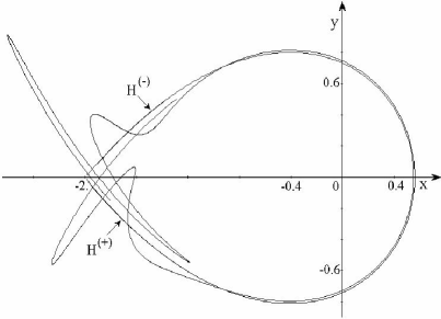
Figure 1: Transversal intersections of stable, $H^{(+)}$, and unstable, $H^{(-)}$, manifolds of the saddle point for $\varepsilon=0.5$ and $\xi=0.01$.

A simplified image of such intersections is given in FIG. 1 where a fragment of the Poincaré section with a small perturbation $\xi=0.01$ in the time moments $2\pi n\,(n=0,\,1,\,2,\ldots)$ for a bunch of trajectories, starting from a neighborhood of the saddle point, is shown. It is a “seed” of Hamiltonian chaos that arises under an arbitrary small perturbation around the unperturbed separatrix loop.

A phase portrait of chaotic advection in our simple flow is shown in FIG. 2. The Poincaré section of passive particle trajectories in FIG. 2a reveals a non-uniformity of the phase space that is typical for Hamiltonian systems with $3/2$ degree of freedom. Fluid around the point vortex placed at ($x=0,\,y=0$) forms a coherent structure, a vortex core, which is filled with regular, almost elliptic orbits. Another large coherent structure is seen to the west from the vortex core, it is filled with regular orbits as well. A magnification of the northern part of this long island is shown in FIG. 2b which demonstrates a chain of small islands along its border line. Further magnification of one of these small islands shown in the inset of FIG. 2b reveals chains of smaller islands and so on. A zone with invariant KAM tori embedded in a stochastic sea, is called the mixing region. While passive particle trajectories just follow streamlines outside the mixing region (in the far downstream and upstream regions) they can be chaotic inside of it.

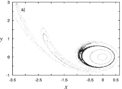
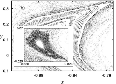
Figure 2: Poincaré section of the mixing region (a), magnification of the northern part of the long island (b), and magnification of the indicated region between the vortex core and the long island in the inset. Parameters are $\varepsilon=0.5$ and $\xi=0.1$.

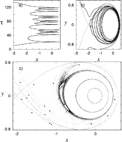
Figure 3: A chaotic wandering of a passive particle initially located at $(x_{0}=-4.358533,\,y_{0}=-6)$ in the mixing region. The time dependence of the $x$ coordinate (a), the particle’s trajectory (b) and the particle’s locations (black circles) on the Poincaré section (c) are shown for $\varepsilon=0.5$ and $\xi=0.1$. The trapping time is $T\simeq 115$.

III Dynamical traps and fractals

Chaotic advection of passive particles in a time-dependent open flow is a typical problem of chaotic scattering. The southern background current with a comparatively small alternating component transports particles along the streamlines into the mixing region, where the particle trajectories can be very complicated and typically chaotic, and then washes out most of them to the north where they again follow the streamlines. We show in this section that in spite of the simplicity of our flow there exists a surprisingly rich variety of different types of trajectories inside the mixing region. Particles with small variations of initial positions are trapped there for trapping times with a broad spectrum extended from a particle transit time with the average velocity of the current to infinity. The dynamical trapping cannot be characterized only by the trapping time $T$, the ways by which advected particles move in the mixing region are very different.

Passive particles are placed outside the mixing region on the line segment with $y_{0}=-6$ and different values of $x_{0\,i}$. We compute the time when the particles reach the line $y=6$ and positions of the particles, $x_{i}(\tau)$ and $y_{i}(\tau)$. The control parameters are chosen to be $\varepsilon=0.5$ and $\xi=0.1$. In FIG. 3 we show the motion of a particle with the initial position $(x_{0}=-4.358533,\,y_{0}=-6)$ trapped in the mixing region for the comparatively long time $T\simeq 115$. In the upper panel of the figure, the dependence of the $x$ coordinate of the particle on time $\tau$ (a) and the particle’s trajectory (b) are shown. The Poincaré plot of the particle positions at the moments of time $\tau=2\pi n$ (black circles) is shown in FIG. 3c. The unperturbed separatrix and the Poincaré section for a collection of particles initially placed inside the mixing region are shown for reference. The particle moves quite uniformly without any preference to visit special zones in the mixing region.

The second particle to be placed initially close to the first one at the point $(x_{0}=-4.358034,\,y_{0}=-6)$ demonstrates cardinally different behavior shown in FIG. 4. It spends in the mixing region much more time, $T\simeq 1581$, than the first particle does. The figure clearly demonstrates the phenomenon of stickiness well-known in chaotic Hamiltonian dynamics D90 ; ZSW ; Z98 . In contrary to the first particle, the second one spends most of time in the mixing region nearby the boundaries of the vortex core and the long island. Motion of the particle in these areas is almost regular with zero maximal Lyapunov exponent. In Hamiltonian systems, there may exist partially broken invariant curves (cantori) in a vicinity of island boundaries which prevent particles to quit the area and act as a kind of permeable barriers. Both these reasons result in stickiness of the islands boundaries that is seen in FIG. 4.

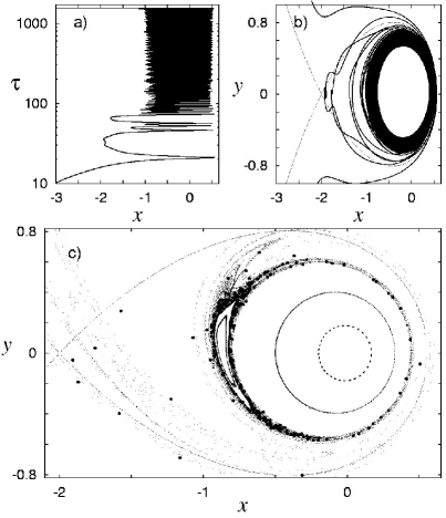
Figure 4: Stickiness of a passive particle initially located at $(x_{0}=-4.358034,\,y_{0}=-6)$ on the boundaries of the vortex core and the long island. The time dependence of the $x$ coordinate (a), the particle’s trajectory (b) and the particle’s locations (black circles) on the Poincaré section (c) are shown for $\varepsilon=0.5$ and $\xi=0.1$. The trapping time $T\simeq 1581$ is very long.

To study the trapping time distribution we have carried out a number of numerical experiments. A trapping map referred to initial positions of $N=22801$ passive tracers, distributed homogeneously on a rectangular grid $(x_{0}\in[-5,\,0];\,y_{0}\in[-6,\,1])$, is shown in FIG. 5.

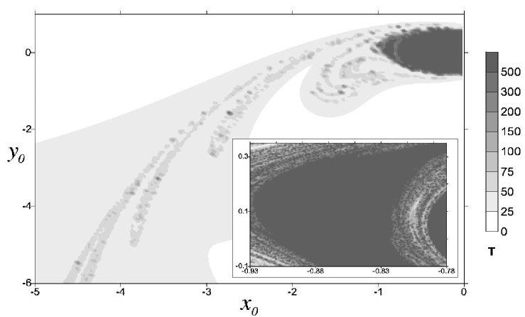
Figure 5: Trapping map showing dependence of the trapping times in the mixing region $T$ on initial positions of $N=22801$ tracers distributed on a rectangular grid in the upstream region. The inset shows a zoom of the fragment of the map.

Color modulates values of the trapping time $T$. The inset shows the respective zone of this map magnified by the factor of $30$ on the $x$ axis and factor of $17$ on the $y$ axis. A patchiness exists for all the scales revealing a fractal-like structure of the underlying phase space. Tracers started initially in the areas of the upstream region, corresponding to black patches on the map, will be trapped in the mixing region for longer times. The inset demonstrates that there exist tracers with very close initial positions whose trapping times differ largely. To quantify this set of dynamical traps with a wide range of trapping times we compute the respective distribution function $N(T)$ for $N=110011$ tracers (positioned initially on a rectangular grid $(x_{0}\in[-4.65,\,-4.35];\,y_{0}\in[-6.05,\,-5.95])$. The double logarithmic plot in FIG. 6 demonstrates initially exponential decay followed by a power-law decay at the PDF tail, $N(T)\sim T^{-\gamma}$, with the characteristic exponent $\gamma\simeq 2$. While a Poissonian distribution is expected for strong chaotic mixing a power-law dependence indicates the presence of dynamical traps in the flow. Particles trapped for longer times give an enhanced contribution to the PDF tail. Different choices of initial positions of the tracers visiting the mixing region do not change significantly the trapping-time distribution.

Figure 6: Trapping time distribution with $N=110011$ tracers shown on $\log-\log$ axes.

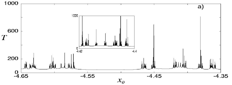
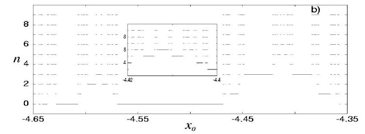
Figure 7: Fractal dependence of the trapping time $T$ on initial particles positions $x_{0}$ with the inset showing a 20-fold magnification of one of the singularity zones (a). Mechanism of generating the fractal with magnification of a small segment corresponding to the inset in the top panel (b).

The well-known manifestation of chaotic scattering is fractal-like scattering functions with an uncountable number of singularities Ott93 ; JZ ; SK96 . We take the trapping time to be the scattering function, $T(x_{0})$, and compute it carefully for $N=10^{4}$ particles distributed initially on the line segment with $y_{0}=-6$ and $x_{0}\in[-4.65,\,-4.35]$. The results in FIG. 7 demonstrate a typical scattering function $T(x_{0})$ with an uncountable number of singularities which are unresolved in principle. The inset in FIG. 7a shows a zoom by the factor of 20 of one of these singularity zones. Successive magnifications confirm a self-similarity of the function with increasing values of the trapping times $T$. FIG. 4 gives an example of a trajectory with very long trapping time $T\simeq 1581$. Remind, please, that we measure time in units of the period of the alternating current. The trapping map in FIG. 5 provides a two-dimensional image of the fractal structure of the scattering function $T(x_{0},\,y_{0})$. As we have shown above, sticky boundaries of islands of regular motion, embedded in a stochastic sea, act as a kind of dynamical traps providing all the spectrum of values of the trapping times up to infinity. Namely these dynamical traps are the ultimate reason for appearing fractals in our simple model flow. To give an insight into a mechanism of generating the fractal we plot in FIG. 7b segments of the initial string with $10^{6}$ tracers which are trapped in the mixing region after $n$ rotations around the fixed point vortex. After each rotation, a portion of tracers is washed out in the downstream region with $y\geqslant 6$. This process resembles the mechanism of generating the famous Cantor set but is more complicated.

In conclusion, we compute the length of the curve $T(x_{0})$ shown in FIG. 7a

$${L\,(1/N)=\sum^{N}_{i=1}|T_{i+1}-T_{i}|,}$$ (9)

as a function of the inverse number of tracers, $N^{-1}$, distributed initially on the same line segment with $y_{0}=-6$ and $x_{0}\in[-4.75,-4.25]$ in the upstream region of the flow. It is a decreasing (in average) function with a negative slope whose double lagarithmic plot is presented in FIG. 8. The Hausdorff dimension of the fractal-like scattering function is computed to be $d\simeq 1.84$.

Figure 8: Length of the fractal curve $T(x_{0})$ versus the inverse number of tracers $N^{-1}$ distributed initially on the same line segment in the upstream region. The double logarithmic plot.

IV Conclusion and discussion

We have shown that chaotic advection of passive particles by the open flow, composed of a fixed point vortex and a background current with a time-dependent component, has a fractal nature. Appearance of fractals and dynamical traps in geophysical flows with topographical vortices should fluence strongly transport and mixing of heat and mass. Instead of homogeneous mixing, one expects a highly-structural, hierarchical fractal distribution of advected particles that is of great interest in oceanography and atmospheric sciences. It should be emphasized that the fractals and dynamical traps are not specific for our particularly simple model. They are typical in low-dimensional Hamiltonian systems and should exist in more realistic models with elliptic topographical vortices and different boundary conditions considered, for example, in KK .

If tracers are not passive but active (chemical reagents or biological species), their activity is superimposed on chaotic mixing in open background flows. Typically, there exists a local coupling between a spatial character of the activity and the spatial character of the fluid with coherent structures, dynamical traps and fractals. Say in chemistry, molecules will react if they are in a close contact with each other. So, the imperfect mixing should largely increases the chemical or biological activity in some regions of the flow and suppress it in other regions. In marine biology, the paradoxical observational fact of coexisting thousands of phytoplankton species in spite of a limited number of resources for which they compete has been known for a long time H61 . Chaotic mixing of active particles in open nonstationary flows in the ocean with small-scale spatial inhomogeneities and fractal patterns can provide a natural explanation of the plankton paradox K00 . Homogeneous and complete mixing leads to an equilibrium state in the system of competing species resulting in the survival of the most fitted species, whereas chaotic mixing generates, typically, a persistent nonequilibrium state in the system providing the coexistence of much more species than the number of ecological niches they occupy.

V Acknowledgments

This work is supported by the Russian Federal Program “World Ocean” in the framework of the Project “Modelling variability of hydrophysical fields” and by the Russian Foundation for Basic Research under project numbers 02-02-17796 and 02-02-06841. We gratefully acknowledge useful discussions with V.F. Kozlov.

References

- (1) V.I. Arnold, Hebd. Seances Acad. Sci. 261 (1965) 17.
- (2) H. Aref, J. Fluid. Mech. 143 (1984) 1.
- (3) J.M. Ottino, The Kinematics of Mixing: Stretching, Chaos and Transport, Cambridge University Press, Cambridge, 1989.
- (4) G.M. Zaslavsky, R.Z. Sagdeev, D.A. Usikov, A.A. Chernikov, Weak Chaos and Quasiregular Patterns, Cambridge University Press, Cambridge, 1991.
- (5) A. Crisanti, M. Falcioni, G. Paladin, A. Vulpiani, La Rivisita del Nuovo Cimento, 14 (1991) 1.
- (6) V.F. Kozlov, Models of the Topographical Vortices in the Ocean, Nauka, Moscow, 1983 [in Russian].
- (7) V.N. Zyryanov, Topographical Vortices in Dynamics of Sea Currents, IVP RAN, Moscow, 1995 [in Russian].
- (8) M.L. Grundlingh, Deep-Sea Res. 24 (1977) 903; L.I. Eide, ibid 26 (1979) 601; W.B. Owens, N.C. Hogg, ibid 27 (1980) 1029; W.J. Gould, R. Hendry, H.E. Huppert, ibid 28 (1981) 409.
- (9) G.I. Taylor, Proc. Roy. Soc. London 104 (1923) 213.
- (10) G.M. Zaslavsky, Physics of Chaos in Hamiltonian Systems, Academic Press, Oxford, 1998.
- (11) V. Rom-Kedar, A. Leonard, S. Wiggins, J. Fluid. Mech. 214 (1990) 347.
- (12) G.M. Zaslavsky, R.Z. Sagdeev, A.A. Chernikov, Zh. Eksp. Teor. Fiz. 94 (1988) 102 [Sov. Phys. JETP 67 (1988) 270].
- (13) A. Péntek et al., Physica A 274 (1999) 120.
- (14) B. Eckhardt, H. Aref, Philos. Trans. R. Soc. London A 326 (1988) 655.
- (15) P. Beyer, S. Benkadda, Chaos 11 (2001) 774.
- (16) C. Jung, E. Ziemniak, J. Phys. A 25 (1992) 3929.
- (17) T.H. Solomon, E.R. Weeks, H.L. Swinney, Phys. Rev. Lett. 71 (1993) 3975.
- (18) J.C. Sommerer, H.-C. Ku, H.E. Gilreath, Phys. Rev. Lett. 77 (1996) 5055.
- (19) T.H. Solomon, S. Tomas, J.L. Warner, Phys. Fluids 10 (1998) 342.
- (20) J. Chaiken, R. Chevray, M. Tabor, W.M. Tam, Proc. R. Soc. London, Ser. A 408 (1987) 165.
- (21) M.V. Budyansky, S.V. Prants, Piśma Zh. Tekh. Fiz. 27 (12) (2001) 51 [Tech. Phys. Lett. 27 (6) (2001) 508].
- (22) E. Ott, Chaos in Dynamical Systems, Cambridge University Press, Cambridge, 1993.
- (23) V.V. Kozlov, Symmetry, Topology and Resonance in Hamiltonian Mechanics, UdGU, Izhevsk, 1995 [in Russian].
- (24) M. Ding, T. Bountis, E. Ott, Phys. Lett. A 151 (1990) 395.
- (25) G.M. Zaslavsky, D. Stevens, H. Weitzner, Phys. Rev. E 48 (1993) 1683.
- (26) V.F. Kozlov, K.V. Koshel, Izv. Rus. Ac. Sci.: Fiz. Atmosp. Ocean 37 (3) (2001) 378 [Izvestiya, Atmospheric and Oceanic Physics 37 (3) (2001) 351].
- (27) G.E. Hutchinson, Amer. Nat. 95 (1961) 1292.
- (28) G. Károlyi et. al., Proc. Natl. Acad. Sci. USA 97 (2000) 13661.