Polychromatic solitons in a quadratic medium

Abstract

We introduce the simplest model to describe parametric interactions in a quadratically nonlinear optical medium with the fundamental harmonic containing two components with (slightly) different carrier frequencies [which is a direct analog of wavelength-division multiplexed (WDM) models, well known in media with cubic nonlinearity]. The model takes a closed form with three different second-harmonic components, and it is formulated in the spatial domain. We demonstrate that the model supports both polychromatic solitons (PCSs), with all the components present in them, and two types of mutually orthogonal simple solitons, both types being stable in a broad parametric region. An essential peculiarity of PCS is that its power is much smaller than that of a simple (usual) soliton (taken at the same values of control parameters), which may be an advantage for experimental generation of PCSs. Collisions between the orthogonal simple solitons are simulated in detail, leading to the conclusion that the collisions are strongly inelastic, converting the simple solitons into polychromatic ones, and generating one or two additional PCSs. A collision velocity at which the inelastic effects are strongest is identified, and it is demonstrated that the collision may be used as a basis to design a simple all-optical XOR logic gate.

I Introduction

Wave mixing at different carrier frequencies, of which generation of higher harmonics is a well-known example, has had a long history of investigation Franken61 ; Armstrong62 . In an optical medium whose symmetry group lacks a center of inversion, the lowest-order nonlinear response is quadratic, which gives rise to three-photon interactions. The resultant three-wave mixing is resonant when the condition $\omega_{3}=\omega_{1}+\omega_{2}$, imposed on frequencies of the three waves, is met. In the particular case when $\omega_{1}=\omega_{2}$, the process reduces to the second harmonic generation (SHG).

Solitons in quadratic [$\chi^{(2)}$] media has been a major area of research recently (see Ref. Etrich01 for a review). The first experimental observation of $\chi^{(2)}$ solitons was reported for type-I SHG, which involves exactly one component of each harmonic, in the $(2+1)$-dimensional (bulk) geometry Torruellas95 . The observation of solitons in the $(1+1)$-dimensional geometry (planar nonlinear waveguide) followed shortly afterwards Schiek96 . Much theoretical work has been performed for the solitons in both type-I and type-II SHG, the latter case involving two components of the fundamental harmonic, corresponding to different polarizations, and a single component of the second harmonic Stegeman ; Buryak95 ; Tran95 ; Malomed96 ; Buryak97 ; JenaTypeII . The SHG process in an isotropic medium, with two polarizations at both harmonics, has been considered too Boardman .

More complex cases of multi-resonance wave mixing in quadratically nonlinear media have not received much attention because of serious difficulties with their experimental realization using the birefringence-based wave-vector matching schemes. However, the recent rapid development of the quasi-phase-matching (QPM) technique has changed the situation. The technique, originally proposed long ago Armstrong62 , relied upon periodic structures (usually, periodically poled ones) with an alternating sign of the quadratic nonlinearity. Recently, the QPM technique has been extended from periodic to Fibonacci-series-based structures Fradkin99 , and further to fully quasiperiodic ones Fradkin02 (see also Ref. Johansen ). This makes it possible to essentially relax conditions on the wave-vector difference for the matching to take place. Results presented in Ref. Fradkin02 show, both theoretically and experimentally, not only high values of effective $\chi^{(2)}$ coefficients, but also that one can attain the wave-vector matching simultaneously for several sets of waves involved in the nonlinear interactions. In particular, the development of the QPM technique has been an incentive to study multi-resonance systems Kivshar99a ; Kivshar99b ; Towers00 ; Sukhorukov01 , a possible application of which may be design of soliton-based logic gates. Indeed, a soliton may naturally be used as a bit of information, and the interactions of solitons can potentially support logic operations.

In this work, we develop a model of nonlinear mixing between two fundamental-harmonic waves with different frequencies in a quadratic medium. Via the $\chi^{(2)}$ nonlinearity, they generate three different wave components of the second harmonic. Note that interactions between waves with different frequencies in optical media with cubic ($\chi^{(3)}$) nonlinearity is a well-known topic, which has extremely important applications to the WDM multichannel format of data transmission in fiber-optic telecommunication links Agrawal ; however, it appears that the issue has not yet been studied for $\chi^{(2)}$ media, in which the mixing may be realized in both spatial and temporal domains.

We formulate the model in section II, and produce its stationary soliton solutions in section III. These may be both fully polychromatic solitons (PCSs), including all the five field components, and special (simple) solutions of “A” and “B” types, which amount to ordinary two-component SHG solitons in mutually orthogonal (non-intersecting) subsets of the five-wave system. In section IV, we demonstrate, by means of direct simulations, that the solitons of all these types are stable in a broad region in the system’s parameter space. In the same section, we simulate collisions between the simple solitons. When they overlap, the nonlinear interaction generates a component which was absent in both of them before the collision, which makes the final result of the collision strongly inelastic: the former simple solitons develop extra components and become polychromatic ones. Additionally, one or two extra solitons are generated by the collision. We demonstrate that the collision between the initial simple solitons may be a basis for an all-optical XOR logic gate. The paper is concluded by section V.

II The model

We consider the interaction of five waves in a diffractive dielectric medium with the quadratic nonlinear susceptibility. The carrier frequencies of the waves satisfy resonant conditions, $\omega_{3}=2\omega_{1},\;\omega_{4}=\omega_{1}+\omega_{2},\;\omega_{5}=2\omega_{2}$, so that $\omega_{1}$ and $\omega_{2}$ may be classified as carriers of the fundamental-harmonic components, while $\omega_{3}$, $\omega_{4}$ and $\omega_{5}$ represent three components of the second-harmonic wave group, generated by the two fundamental-harmonic components via the $\chi^{(2)}$ nonlinearity.

Assuming, as usual, that the wave envelopes $E_{1},E_{2}$ and $E_{3},E_{4},E_{5}$ of these components are slowly varying ones, a system of five equations, coupled parametrically through the components of the $\chi^{(2)}$ nonlinear susceptibility tensor, can be derived from the Maxwell’s equations to govern the evolution of the waves in the spatial domain (the derivation follows the well-known procedure worked out for the usual type-I and type-II $\chi^{(2)}$ interactions, see a detailed account given in the review Etrich01 ):

$$2ik_{1}\frac{\partial E_{1}}{\partial z}+\frac{\partial^{2}E_{1}}{\partial x^{2}}+2\tilde{\chi}_{1}E_{1}^{\ast}E_{3}e^{i\Delta k_{3,1,1}}+\sqrt{2}\tilde{\chi}_{2}E_{2}^{\ast}E_{4}e^{i\Delta k_{412}} = 0,$$

$$2ik_{2}\frac{\partial E_{2}}{\partial z}+\frac{\partial^{2}E_{2}}{\partial x^{2}}+\sqrt{2}\tilde{\chi}_{2}E_{1}^{\ast}E_{4}e^{i\Delta k_{412}}+2\tilde{\chi}_{3}E_{2}^{\ast}E_{5}e^{i\Delta k_{522}} = 0,$$

$$2ik_{3}\frac{\partial E_{3}}{\partial z}+\frac{\partial^{2}E_{3}}{\partial x^{2}}+\tilde{\chi}_{1}E_{1}^{2}e^{-i\Delta k_{311}} = 0,$$ (1)

$$2ik_{4}\frac{\partial E_{4}}{\partial z}+\frac{\partial^{2}E_{4}}{\partial x^{2}}+\sqrt{2}\tilde{\chi}_{2}E_{1}E_{2}e^{-i\Delta k_{412}} = 0,$$

$$2ik_{5}\frac{\partial E_{5}}{\partial z}+\frac{\partial^{2}E_{5}}{\partial x^{2}}+\tilde{\chi}_{3}E_{2}^{2}e^{-i\Delta k_{522}} = 0,$$

where $k_{1}$ through $k_{5}$ are the corresponding carrier wave numbers, $z$ and $x$ are the propagation and transverse coordinates, $\Delta k_{lmn}=k_{l}-k_{m}-k_{n}$ is the wave-vector mismatch, and $\tilde{\chi}_{n}\equiv 8\pi\omega_{n}^{2}/c^{2}\chi^{(2)}$, $\chi^{(2)}$ being an element of the quadratic susceptibility tensor. The extra factors of $2$ in front of the coefficients $\tilde{\chi}_{1}$ and $\tilde{\chi}_{3}$ in the first two equations reflects the fact the equations may be derived from a Lagrangian, and the factor $\sqrt{2}$ in front of all the terms containing $\tilde{\chi}_{2}$ is added by definition, to simplify subsequent rescalings.

Equations (1) are normalized by measuring $x$ and $z$, respectively, in units of the input beam size $r_{0}$ and diffraction length $z_{d}=r_{0}^{2}k_{4}$ at the frequency $\omega_{1}+\omega_{2}$. Introducing dimensionless fields

$$E_{1} = (u_{1}/\sqrt{2}\gamma)\exp\left(i\beta_{1}z\right),E_{2}=(u_{2}/\sqrt{2}\gamma)\exp\left(i\beta_{2}z\right),E_{3}=(u_{3}/2\gamma)\exp\left(2i\beta_{1}z-i\Delta k_{311}z\right),$$ (2)

$$E_{4} = (u_{4}/\sqrt{2}\gamma)\exp\left(i(\beta_{1}+\beta_{2})z-i\Delta k_{412}z\right),E_{5}=(u_{5}/2\gamma)\exp\left(2i\beta_{2}z-i\Delta k_{522}\right),$$ (3)

and $\gamma\equiv\tilde{\chi}_{1}r_{0}^{2}$, a normalized system of equations is obtained:

$$2\frac{k_{1}}{k_{4}}\left(i\frac{\partial u_{1}}{\partial z}-\beta_{1}u_{1}\right)+\frac{\partial^{2}u_{1}}{\partial x^{2}}+\chi_{1}u_{1}^{\ast}u_{3}+\chi_{2}u_{2}^{\ast}u_{4} = 0,$$

$$2\frac{k_{2}}{k_{4}}\left(i\frac{\partial u_{2}}{\partial z}-\beta_{2}u_{2}\right)+\frac{\partial^{2}u_{2}}{\partial x^{2}}+\chi_{2}u_{1}^{\ast}u_{4}+\chi_{3}u_{2}^{\ast}u_{5} = 0,$$

$$2\frac{k_{3}}{k_{4}}\left(i\frac{\partial u_{3}}{\partial z}-\left(2\beta_{1}-\Delta k_{311}\right)u_{3}\right)+\frac{\partial^{2}u_{3}}{\partial x^{2}}+\frac{1}{2}\chi_{1}u_{1}^{2} = 0,$$ (4)

$$2\frac{k_{4}}{k_{4}}\left(i\frac{\partial u_{4}}{\partial z}-\left(\beta_{1}+\beta_{2}-\Delta k_{412}\right)u_{4}\right)+\frac{\partial^{2}u_{4}}{\partial x^{2}}+\chi_{2}u_{1}u_{2} = 0,$$

$$2\frac{k_{5}}{k_{4}}\left(i\frac{\partial u_{5}}{\partial z}-\left(2\beta_{2}-\Delta k_{522}\right)u_{5}\right)+\frac{\partial^{2}u_{5}}{\partial x^{2}}+\frac{1}{2}\chi_{3}u_{2}^{2} = 0.$$

where $\chi_{n}\equiv\tilde{\chi}_{n}/\tilde{\chi}_{1}$ ($n=1,2,3$, i.e., $\chi_{1}\equiv 1$), $\beta_{1,2}$ being two phase-velocity shifts. To reduce the number of parameters in Eqs. (4), the fields and coordinates can be rescaled further. Defining $u_{n}=\beta_{1}U_{n}$, $z=Z/\beta_{1}$ , and $x=X/\sqrt{|\beta_{1}|}$, we obtain

$$i\frac{\partial U_{1}}{\partial Z}+\frac{\partial^{2}U_{1}}{\partial X^{2}}-\alpha_{1}U_{1}+\chi_{1}U_{1}^{\ast}U_{3}+\chi_{2}U_{2}^{\ast}U_{4} = 0,$$

$$i\frac{\partial U_{2}}{\partial Z}+\frac{\partial^{2}U_{2}}{\partial X^{2}}-\alpha_{2}U_{2}+\chi_{2}U_{1}^{\ast}U_{4}+\chi_{3}U_{2}^{\ast}U_{5} = 0,$$

$$2i\frac{\partial U_{3}}{\partial Z}+\frac{\partial^{2}U_{3}}{\partial X^{2}}-\alpha_{3}U_{3}+\frac{1}{2}\chi_{1}U_{1}^{2} = 0,$$ (5)

$$2i\frac{\partial U_{4}}{\partial Z}+\frac{\partial^{2}U_{4}}{\partial X^{2}}-\alpha_{4}U_{4}+\chi_{2}U_{1}U_{2} = 0,$$

$$2i\frac{\partial U_{5}}{\partial Z}+\frac{\partial^{2}U_{5}}{\partial X^{2}}-\alpha_{5}U_{5}+\frac{1}{2}\chi_{3}U_{2}^{2} = 0.$$

where $\alpha_{1}=1$, $\alpha_{2}=\beta_{2}/\beta_{1}$, $\alpha_{3}=(4\beta_{1}-2\Delta k_{311})/\beta_{1}$, $\alpha_{4}=(2\beta_{1}+2\beta_{2}-2\Delta k_{412})/\beta_{1}$, and $\alpha_{5}=(4\beta_{2}-2\Delta k_{522})/\beta_{1}$. We assume that $\left|k_{4}-k_{2}-k_{1}\right|\ll k_{n}$, and everywhere, except for the phase-mismatch parameters introduced above, one may set $k_{3}=k_{4}=k_{5}$, i.e., the three components of the second-harmonic wave have similar wave numbers.

Equations (5) assume that the three parametric interactions (“vertices”), which couple, respectively, the wave triplets (1,1,3), (2,2,5), and (1,2,4), are nearly phase matched (as it was mentioned above, a possible way of achieving this may be provided by the QPM technique based on quasiperiodic structures Fradkin02 ). It is straightforward to see that, like the model describing the type-II SHG Tran95 ; Malomed96 ; Buryak97 , Eqs. (5) have two Manley-Rowe invariants, namely, the total power,

$$Q=\int_{-\infty}^{\infty}|U_{1}|^{2}+|U_{2}|^{2}+4\left(|U_{3}|^{2}+|U_{4}|^{2}+|U_{5}|^{2}\right)dx,$$ (6)

and the power imbalance,

$$Q_{{\rm imb}}=\int_{-\infty}^{\infty}|U_{1}|^{2}-|U_{2}|^{2}+4\left(|U_{3}|^{2}-|U_{5}|^{2}\right)dx.$$ (7)

The present model does not include walkoff terms (group-velocity mismatch). While a detailed discussion of the walkoff is beyond the scope of this work, it is relevant to mention that QPM and similar techniques, such as tandem structures tandem , make it possible to suppress the walkoff tandem ; Stolzenberger . We also note that QPM can give rise to an effective cubic nonlinearity Clausen , which may compete with the underlying quadratic interactions Bang ; Johansen . For this reason, cubic terms should sometimes be added to a dynamical model, but this is not an issue for immediate consideration in the present context. As concerns the physical realization of the system, estimates using typical values of the relevant physical parameters in such quadratically nonlinear materials as lithium niobate and KTP Fradkin02 ; Johansen suggest that a necessary (quasi) period of the QPM structure is $\ \sim 10$ $\mu$m, and the power and transverse  size of the soliton beam are expected to be $\,\sim 20$ $\mu$m and $100$ mW, respectively.

If still more resonances are allowed, other essential wave components may appear, for instance, those corresponding to the combinational frequencies $\omega_{12}\equiv 2\omega_{1}-\omega_{2}$ and $\omega_{21}\equiv 2\omega_{2}-\omega_{1}$ (obviously, they belong to the fundamental-harmonic wave set). Denoting the corresponding wave numbers as $k_{12}$ and $k_{21}$, we see that these new components will indeed be essential if the wave-number triplets (12,2,3) and/or (21,1,5) are nearly phase-matched. The accordingly modified system will include seven components (four pertaining to the fundamental harmonic, and three to the second harmonic) and five vertices. However, such a situation seems much more exotic (five simultaneous resonances) than the more generic possibility of three simultaneous resonances underlying the model considered in the present work.

III Stationary soliton solutions

Particular exact solutions of Eqs. (5) for stationary solitons can be sought for in the form

$$U_{n}=A_{n}{\rm sech}^{2}\left(\lambda X\right),\,n=1,...,5,$$ (8)

where $A_{n}$ are amplitudes, and $\lambda$ is the inverse width of the soliton. Inserting this (8) into Eqs. (5), a solution can be obtained if $\alpha_{1}=\alpha_{2}=\alpha_{3}=\alpha_{4}=\alpha_{5}\equiv\alpha$ and $\lambda=\sqrt{\alpha}/2$. The amplitudes are found to be

$$A_{1} = \pm\sqrt{\xi}A_{2},\,A_{2}=\pm\frac{6\lambda^{2}}{\chi_{2}^{2}\xi+\chi_{3}^{2}/2},\,A_{3}=\frac{\chi_{1}A_{1}^{2}}{12\lambda^{2}},$$

$$A_{4} = \frac{\chi_{2}A_{1}A_{2}}{6\lambda^{2}},\,A_{5}=\frac{\chi_{3}A_{2}^{2}}{6\lambda^{2}},$$ (9)

where $\xi\equiv(\chi_{3}^{2}/2-\chi_{2}^{2})/(\chi_{1}^{2}/2-\chi_{2}^{2})$.

In addition to the exact solution based on Eqs. (8) and (9), other particular solutions can be found setting $U_{2,4,5}=0$ or, alternatively, $U_{1,3,4}=0$. Equations (5) then reduce to the well-known type-I SHG model Stegeman ; Buryak95 ; Etrich01 ,

$$i\frac{\partial V}{\partial Z}+\frac{\partial^{2}V}{\partial X^{2}}-V+V^{\ast}W = 0,$$ (10)

$$2i\frac{\partial W}{\partial Z}+\frac{\partial^{2}W}{\partial X^{2}}-\rho W+\frac{1}{2}V^{2} = 0,$$ (11)

where $V$ and $W$ are the fields at the fundamental and second harmonics. In this case, there is a well-known special exact solution corresponding to $\rho=1$ in Eq. (11) Karamzin74 ,

$$V=\left(3/\sqrt{2}\right){\rm sech}^{2}\left(X/2\right),\,W=\left(3/2\right){\rm sech}^{2}\left(X/2\right).$$

When $\rho\neq 1$, a family of stationary soliton solutions to Eqs. (10) and (11) can be found numerically Buryak95 (or approximated analytically by means of the variational method Vika ). We will refer to the general solution for the case when $U_{1}=V$, $U_{3}=W$, and $U_{2,4,5}=0$ as an “A” type soliton, while the opposite “B” type is defined as the one with $U_{2}=V$, $U_{5}=W$, and $U_{1,3,4}=0$. Both these types will also be called “simple” solitons.

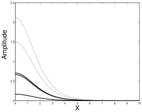
Figure 1: Profiles of a polychromatic soliton (solid lines) and a type “A” soliton (dotted). Common values of the parameters for these solutions are $\alpha_{1,...,5}=1$, $\chi_{1}=1$, $\chi_{2}=2$, and $\chi_{3}=1$.

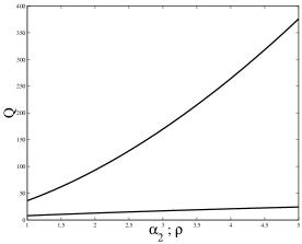
Figure 2: The power invariant $Q$ for both the “A”-type (upper line, vs. $\rho$) and full polychromatic (lower line, vs. $\alpha_{2}$) solitons. Values of the parameters are the same as in Fig. 1.

General solutions for the polychromatic (five-wave) soliton can be found from the stationary version (the one with $\partial U_{n}/\partial Z=0$) of Eqs. (5) by means of the standard numerical methods for two-point boundary-value problems. In Figs. 1 and 2, comparison is made between the general five-wave solitons and the particular solutions generated by Eqs. (10) and (11) at equal values of all the parameters. In Fig. 1, one can see that the A soliton is much larger in amplitude, while its width is not widely different from that of the polychromatic one. As a consequence of this, the power $Q$ [see Eq. (6)] of the A-type soliton shown in Fig. 1 is $Q=36$, while for PCS in the same figure, $Q=8$ [the other invariant is $Q_{{\rm imb}}=0$ in the case considered, see Eq. (7)].

This drastic difference in the powers can be understood: in the case of the full PCS, one has two nonlinear terms in the first two equations (5), rather than one term in the case of the simple solitons; therefore, the amplitude necessary to compensate the spreading out of the beam due to the diffraction term is, roughly, twice as small in comparison with the simple solitons, or, eventually, the power is $\,\sim 4$ times as small. To check whether the power of the PCS is indeed essentially lower than that of simple solitons in the general case, in Fig. 2 we show a typical example of the change of the two powers with the variation of $\alpha_{2}$ or, equivalently, $\rho$ in Eq. (11). As is seen, PCS indeed persistently maintains a lower power $Q$ than its A-type counterpart. On varying the different parameters $\alpha_{n},\chi_{n}$ the value of $Q$ of the polychromatic soliton may be increased (or decreased) in value from that portrayed in Fig. 2 but it only exceeds that of the simple solitons when $\chi_{2}<0.7$. In the limit of $\chi_{2}\rightarrow 0$ Eqs. (5) decouple and the polychromatic soliton tends to a “double” simple soliton i.e. both “A” and “B” type solitons existing in one envelope. The double simple soliton by definition has twice the power of single simple soliton. Provided the nonlinearity coefficient $\chi_{2}$ is large enough ($\chi_{2}\geq 0.7$) it is possible to conclude that PCSs in a quadratically nonlinear medium may be produced from waves with different frequencies at a much lower net input power than the ordinary SHG solitons, i.e., it may be essentially easier to generate PCSs in the experiment and use them in potential applications. Of course, these results are meaningful provided that these solitons are stable.

IV Stability and interactions of the solitons

IV.1 The stability of the polychromatic solitons

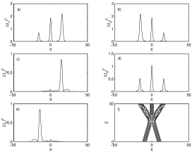
Figure 4: The collision between simple solitons of the mutually orthogonal A and B types, with the initial velocities $\pm 0.3$ and zero phase difference. The parameters are $\alpha_{n}=1$, $\chi_{1}=\chi_{3}=1$, $\chi_{2}=2$, and $C=0.3$. The field components are displayed in the panels: $U_{1}$ (a), $U_{2}$ (b), $U_{3}$ (c), $U_{4}$ (d), and $U_{5}$ (e). The panel (f) shows a combined contour plot of the $U_{1}$ and $U_{2}$ amplitudes. Note the mirror symmetry of the profiles of the components $U_{1}$ and $U_{2}$, which is a consequence of the fact that the imbalance invariant $Q_{imb}$ is zero in this case. It is obvious that the simple solitons become polychromatic after the collision, and the third polychromatic soliton with the zero velocity is generated.

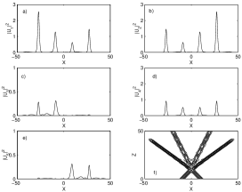
Figure 5: The same as in Fig. 4, except that the collision velocities are larger, $\pm 1.0$. A zero-velocity soliton is no longer generated after the collision. Instead, four solitons are observed in the post-collision state. In the panel (f) the outer beams terminate prematurely because they hit the absorbing sponges used in the numerical scheme.

To test the stability of PCSs, we solved the full system of Eqs. (5), employing the numerical split-step fast-Fourier-transform method. The simulations were performed with a computational grid of 2048 points, the transverse and propagation step-sizes being, respectively, $h_{x}\approx 0.02$ and $h_{z}=0.01$. The integration domain had the transverse size $100$ ($-50<x<+50$), which is by far larger than any $x$ size relevant to the solitons, see Figs. 4, 5, and 9 below. Absorbing layers were placed at the edges of the computational domain to prevent reentering of radiation. Specially monitoring interaction of the radiation waves with the absorbers, we have verified that, in all the cases considered, no reflection took place indeed.

Evolution of initial configurations close to the stationary solutions was simulated for a variety of parameters. To impose initial perturbations, values of the initial amplitude and width of the pulses were altered against the exact stationary solutions. From the results of the simulations, we have concluded that PCSs survive, clearly remaining stable, as long as the simulations were run, the maximum simulation length being 300 diffraction lengths of the soliton.

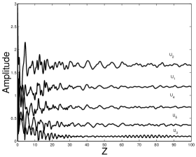
Figure 3: The generation of a polychromatic soliton from the Gaussian input $U_{1}=2e^{-x^{2}/4}$ and $U_{2}=3e^{-x^{2}/4}$. After an initial period of strong relaxation, a weakly oscillating soliton is produced. The evolution of the amplitudes of the $U_{n}$ components vs. $Z$ is plotted. The parameters used in this simulation were $\alpha_{1}=\alpha_{2}=1$, $\alpha_{3}=\alpha_{4}=\alpha_{5}=4$, $\chi_{1}=\chi_{3}=1$, and $\chi_{2}=2$. The power invariants are $Q=13\sqrt{2\pi}$ and $Q_{imb}=-5\sqrt{2\pi}$.

To further test robustness of PCSs, we ran numerical experiments in which the solitons were successfully generated from initial Gaussian pulses, launched in the pump fields $U_{1}$ and $U_{2}$ (with no initial second-harmonic components, which corresponds to the generation of SHG solitons in real experiments Stegeman_experiment ). The results demonstrate that PCSs not only are stable against small perturbations, but also play the role of strong attractors in the system. An example of PCS generation from the Gaussian beams is illustrated by Fig. 3. Typically, there is a period of strong relaxation of the beams, where the amplitudes fluctuate and excess energy is radiated away. The second-harmonic components $U_{3,4,5}$ are generated, and the soliton arranges itself to a quasi-stationary form, which then propagates, in a stable fashion, over a distance in excess of 100 diffraction lengths (as long as the simulations were run). As a result of many runs of systematic simulations, PCSs have been found to be attractors in a broad range in the system’s parameter space. We concentrated mainly on the parameter space $\alpha_{n}=1..5$ and $\chi_{n}=1..2$ where the PCS definitely had a lower value $Q$ than the simple solitons. In connection to this, it is relevant to note that the above-mentioned families of the simple A and B solitons are also stable in the ordinary SHG model, except for a small region of their existence domain Buryak95 ; Etrich01 .

IV.2 Collisions between orthogonal simple solitons

An interesting possibility is to consider collisions of the mutually orthogonal simple solitons of the above-mentioned A and B types. The overlapping between the colliding solitons will give rise to the generation of the field $U_{4}$, which is absent in both A and B solitons in their pure form, and the issue is how the generation of this field will affect the interaction between the solitons. Equations (11) have the property of the Galilean invariance, so “moving” solitons (in fact, the solitary beams propagating at an angle in the planar waveguide) can be constructed by the transformation

$$V(X,Z) = V_{0}\left(X-CZ\right)\exp\left(iCX/2-iC^{2}Z/4\right)\,,$$ (12)

$$W(X,Z) = W_{0}\left(X-CZ\right)\exp\left(iCX-iC^{2}Z/2\right)\,,$$

where $C$ is the “velocity” (actually, a slope) of the “moving” soliton.

We collided the A and B solitons with an initial separation between their centers $x_{0}=20$, varying their velocities $\pm C$. A representative set of values of the parameters for which the results are displayed below are $\alpha_{1,...,5}=1$, $\chi_{1}=\chi_{3}=1$, and $\chi_{2}=2$; many simulations run for other values gave quite similar results.

In the case of moderate collision velocities (and zero phase difference between the solitons), the generation of the field $U_{4}$ in the course of the collision gives rise to a third polychromatic soliton with the zero velocity. Trajectories of the initial A and B solitons alter, and they appear from the collisions as PCSs too, i.e., the collision adds to them components which were initially absent. The three post-collision solitons have roughly equal powers, with a mirror symmetry in the power distribution amongst individual components, see Fig. 4. At higher collision velocities (again, for the zero phase difference), four PCSs are generated by the collision, all having a nonzero velocity (see Fig. 5). As the collision velocity increases, less and less interaction takes place, until the initial solitons pass through one another unchanged (elastically). In all these cases, 90$\%$ of the initial power is typically converted into the resulting PCSs, i.e., radiation loss is not a dominant actor in the collision dynamics.

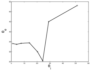
Figure 6: The exit angle (in degrees) $\theta_{{\rm e}}$ for the outer solitons, as found from the simulations of the collision, vs. the incidence angle $\theta_{{\rm i}}$. The angles are between the solitons’ trajectories and the $z$ axis in the $(x,z)$ plane, so that an increase in the incidence angle corresponds to an increase in the collision velocity. Naturally, the collision becomes less inelastic as $\theta_{{\rm i}}$ increases, and eventually the exit angle becomes nearly equal to the incidence one.

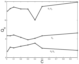
Figure 7: Distribution of the powers $Q_{n}=\int_{-\infty}^{\infty}|U_{n}|^{2}dx$ between the components of the former A or B soliton after the collision, as a function of the soliton velocity before the collision. At higher velocities, the collision gives rise to 4 (rather than 3) solitons, which take a part of the energy.

Results produced by many runs of the simulations for the collision of the in-phase (zero-phase-difference) solitons are summarized in Figs. 6 and 7. The constant initial separation $x_{0}$ between the solitons in the simulations means that the increasing velocity corresponds to an increasing incidence angle $\theta_{{\rm i}}$. As may be naturally expected, the collision alters the trajectories of the solitons most in the case of low velocities. At higher velocities, the outer solitons keep essentially the same velocity after the collision as they had before it, while the two additionally generated inner solitons are significantly slower.

The most significant inelastic effects occur when the solitons collide with the velocities $\pm 0.4$. In this case, the exit trajectory is altered the most (see Fig. 6), and, as per Fig. 7, the largest part of the net power is transferred into the newly generated harmonic components of the outer solitons.

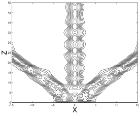
Figure 8: The combined amplitude contour plot of the pump waves $U_{1}$ and $U_{2}$ in the case when the initial velocities of the simple solitons “A” and “B” are zero.

The interaction between the A and B solitons produces nontrivial results also in the case when they have zero initial velocities, but their tails overlap at the initial position. For the initial separation $x_{0}=5$, the result of the interaction with $C=0$ is displayed in Fig. 8, in the form of the distribution of the fields $U_{1}$ and $U_{2}$ produced by the interaction. Again, three PCSs appear, the central one with the zero velocity, and two outer solitons with nonzero velocities. In the course of the evolution, a phase difference develops across the component fields. In fact, it is this phase difference which repulses the outer solitons, lending them a nonzero velocity.

It is well known from theoretical Stegeman_theory and experimental Stegeman_experiment studies of collisions between SHG solitons of the usual type that the result strongly depends on their relative phase at the collision point (provided that the colliding solitons have nearly identical amplitudes): they attract each other and therefore interact strongly in the case of the zero phase difference, and repel each other if the phase difference between the fundamental-harmonic components is $\pi$. However, in the present system the effect of the phase difference on collisions between the simple solitons of the orthogonal types is much weaker. Simulations performed with various phase differences (including $\pi/2$) between the two orthogonal simple solitons does not display any change in the post-collision dynamics of the beams when compared to the zero phase difference case. Also it may be seen from the structure of the underlying system (5) that phase differences between the “A” and “B” solitons will have little effect. Indeed, these equations are exactly invariant against the transformation $u_{1}\rightarrow u_{1}\exp\left(i\phi_{1}\right)$, $u_{3}\rightarrow u_{3}\exp\left(2i\phi_{1}\right)$, $u_{2}\rightarrow u_{2}\exp\left(i\phi_{2}\right)$, $u_{5}\rightarrow u_{5}\exp\left(2i\phi_{2}\right)$ and $u_{4}\rightarrow u_{4}\exp\left(i\phi_{1}+i\phi_{2}\right)$ with an arbitrary phase shift $\phi_{1,2}$.

The interactions between the simple solitons in this system may find application as a basis for an all-optical logic gate. Indeed, consider two solitons of the “A” and/or “B” types, propagating in such a way that they will collide. If the solitons belong to the same type (i.e., the configuration is AA or BB), then they attract or repel one another, depending on their relative phase Stegeman_experiment ; Stegeman_theory , or, if the relative velocity is high enough, they simply pass through one another. But if they belong to the opposite types (an AB configuration), at least three PCSs are produced by the collision even at high velocities. This is a behavior which is expected from an exclusive OR gate, alias XOR. The actual outcome can be easily established by checking the $U_{4}$ content in the output (by means of an appropriate optical filter). An advantage of such a design of the XOR gate is that any output beam will be a stationary soliton (even in the case of a strongly inelastic collision), which makes it convenient for further manipulations (cascadability).

V Conclusion

We have introduced the simplest five-component model of polychromatic solitons (PCSs) in a quadratically nonlinear optical medium. The existence and stability of both polychromatic and two types of simple solitons have been demonstrated. An essential peculiarity of PCSs is that their power is much smaller, at the same values of the control parameters, than the power of the usual two-component (simple) solitons. We have also performed systematic simulations of collisions between mutually orthogonal simple solitons, concluding that the collisions are strongly inelastic (including the interaction between two solitons with the zero initial velocity), giving rise to transformation of the simple solitons into polychromatic ones, and generation of one or two additional PCSs. A value of the relative velocity at which the inelastic effects are strongest has been found. We have also shown that the collision may serve as a basis to design a simple all-optical logic gate of the XOR type.

- (1) P.A. Franken, A.E. Hill, C.W. Peters, and G. Weinreich, Phys. Rev. Lett. 7, 118 (1961).
- (2) J.A. Armstrong, N. Bloembergen, J. Ducuing, and P.S. Pershan, Phys. Rev. 127, 1918 (1962).
- (3) C. Etrich, F. Lederer, B.A. Malomed, T. Peschel, and U. Peschel, Progr. Optics 41, 483 (2000).
- (4) W.E. Torruellas, Z. Wang, D.J. Hagan, E.W. Van Stryland, G.I. Stegeman, L. Torner, and C.R. Menyuk, Phys. Rev. Lett. 74, 5036 (1995).
- (5) R. Schiek, Y. Baek, and G.I Stegeman, Phys. Rev. E53, 1138 (1996).
- (6) C.R. Menyuk, R. Schiek, and L. Torner, J. Opt. Soc. Am. B 11, 2434 (1994).
- (7) A.V. Buryak and Y.S. Kivshar, Phys. Lett. A 197, 407 (1995).
- (8) H.T. Tran, Opt. Commun. 118, 581 (1995).
- (9) B.A. Malomed, D. Anderson, and M. Lisak, Opt. Commun. 126 251 (1996).
- (10) A.V. Buryak, Y.S. Kivshar, and S. Trillo, J. Opt. Soc. Am. B14, 3110 (1997).
- (11) U. Peschel, C. Etrich, F. Lederer, and B.A. Malomed, Phys. Rev. E55, 7704 (1997).
- (12) A.D. Boardman, P. Bontemps, and K. Xie, Opt. Quant. Electron. 30, 891 (1998).
- (13) K. Fradkin-Kashi and A. Arie, IEEE J. Quantum Electron. 35, 1649 (1999).
- (14) K. Fradkin-Kashi, A. Arie, P. Urenski, and G. Rosenman, Phys. Rev. Lett. 88, 023903 (2002).
- (15) S.K. Johansen, S. Carrasco, L. Torner, and O. Bang, Opt. Commun. 203, 393 (2002).
- (16) Y.S. Kivshar, T.J. Alexander, and S. Saltiel, Opt. Lett. 24, 759 (1999).
- (17) Y.S. Kivshar, A.A. Sukhorukov, and S. M. Saltiel, Phys. Rev. E60, R5056 (1999).
- (18) I. Towers, A.V. Buryak, R.A. Sammut, and B.A. Malomed, J. Opt. Soc. Am. B17, 2018 (2000).
- (19) A.A. Sukhorukov, T.J. Alexander, Y.S. Kivshar, and S.M. Saltiel, Phys. Lett. A 281, 34 (2001).
- (20) G.P. Agrawal. Nonlinear Fiber Optics (Academic Press: San Diego, 1995).
- (21) L. Torner, IEEE Photonics Techn. Lett. 11, 1268 (1999).
- (22) R. Stolzenberger, Lasers & Optronics 19, 17 (2000).
- (23) C. B. Clausen, O. Bang and Y. S. Kivshar, Phys. Rev. Lett. 78, 4749 (1997).
- (24) O. Bang, C.B. Clausen, P.L. Christiansen, and L. Torner, Opt. Lett. 24, 1413 (1999); O. Bang, T.W. Graversen, and J.F. Corney, Opt. Lett. 26, 1007 (2001).
- (25) Y.N. Karamzin and A.P. Sukhorukov, JETP Lett. 20, 339, (1974).
- (26) V. Steblina, Yu.S. Kivshar, M. Lisak, and B.A. Malomed, Opt. Commun. 118 345, (1995).
- (27) R. Schiek, Y. Baek, G. Stegeman, and W. Sohler, Opt. Quant. Electr. 30, 861 (1998).
- (28) D.M. Baboiu and G.I. Stegeman, Opt. Quant. Electr. 30, 849 (1998).