Averages and critical exponents in type-III intermittent chaos

Abstract

The natural measure in a map with type-III intermittent chaos is used to define critical exponents for the average of a variable from a dynamical system near bifurcation. Numerical experiments were done with maps and verify the analytical predictions. Physical experiments to test the usefulness of such exponents to characterize the nonlinearity at bifurcations were done in a driven electronic circuit with diode as nonlinear element. Two critical exponents were measured: $\nu=0.55$ for the critical exponent of the average of the voltage across the diode and $\beta=0.62$ for the exponent of the average length of the laminar phases. Both values are consistent with the predictions of a type-III intermittency of cubic nonlinearity. The averages of variables in intermittent chaotic systems is a technique complementary to the measurements of laminar phase histograms, to identify the nonlinear mechanisms. The averages exponents may have a broad application in ultrafast chaotic phenomena.

DOI 10.1103/PhysRevE.66.026210

PACS numbers: 0.5.45.-a, 84.30.Bv

I Introduction

Intermittent chaos is the phenomenon shown by systems exhibiting long sequences of periodic-like behaviour, the laminar phases, separated by comparatively short chaotic eruptions. Intermittent chaotic systems have been extensively studied since the original proposals by Pomeau and Manneville pomeau80 ; berge84 ; manneville90 ; kim98 classifying type-I, II, and III instabilities when the Floquet multipliers of a map crosses the unity circle. Although other mechanisms may occur leading to intermittency these three cases are the most simple and most frequently encountered in low dimensional systems. The class of intermittent chaos studied by Pomeau and Manneville includes the tangent bifurcation, leading to intermittency of type I, when the Floquet’s Multiplier for the associated map crosses the circle of complex numbers with unitary norm through $+1$; the Hopf bifurcation, leading to type-II intermittency, which appears as two complex eigenvalues of the Floquet’s Matrix cross the unitary circle off the real axis; and the sub-critical period doubling, leading to type-III intermittency, whose critical Floquet’s Multiplier is $-1$.

Many experimental evidences for these intermittent behavior have appeared in the literature. The type-III has been reported for electronic nonlinear devices jeffries82 ; fukushima88 ; ono95 , lasers tang91 , and biological tissues griffith97 . A signature for this intermittency is given by the critical exponent describing the dependence of average length of nearly periodic phases, that is, laminar phases, with the control parameter. Histograms of number of laminar phases longer than a given duration are related to the normal form nonlinearity describing the system berge84 ; kodama91 . Different nonlinear power in the model imply different exponents, as described by Kodama et al. kodama91 . Kim et al. kim98 studied the exponent for the average length of laminar phases as function of the reinjection probability. Herein another average is explored to characterize the intermittency and its nonlinearity. It is the average of one variable of the system. Near bifurcation, approximate expressions for the natural measure, or probability density, are obtained for a map with type-III intermittency, in section II. Critical exponents are defined from analytical approximations and shown to be useful in characterizing the bifurcation.

Numerical experiments with the maps are presented in section III, verifying the proposed exponents. To test in a real physical system, a nonlinear circuit with a diode, similar to the one used in the early demonstrations of chaotic universal properties jeffries82 ; linsay81 ; testa82 ; buskirk85 , was set up as described in section IV and used to verify the exponents. The voltage across the diode, which is a dynamical variable of the system, was simultaneously measured in time series and average. The type-III intermittency bifurcation is well characterized both, using the experimental next peak value map and the average.

II Normal Form map with type-III intermittency

To establish the new critical exponents for the averages one begins with the normal form of the map that has type-III intermittency berge84

$$M(X)=-(1+\epsilon^{\prime})X+\alpha X^{2}+\eta^{\prime}X^{3}$$ (1)

The bifurcation, when $X=0$ ceases to be a stable fixed point, occurs at $\epsilon^{\prime}=0$. The second application of this map, in the approximation of small $\epsilon^{\prime}$ and X is given by

$$M^{2}(X)=(1+2\epsilon^{\prime})X+\eta X^{3}$$ (2)

where $\eta=-2(\eta^{\prime}+\alpha^{2})$. If this coefficient is positive and $\epsilon^{\prime}>0$ one has type-III intermittency around $X=0$, provided a reinjection mechanism is introduced in eqs. (1) and (2). When $\alpha\neq 0$ the map of eq. (1) is nonsymmetrical in $X$. Generally, any odd exponent in the nonlinear term of eq. (2) leads to the intermittency. Thus, a map (second iterate) defined in the interval $[0,1]$ with the type-III intermittency is manneville90

$$X_{n+1}=\left[(1+\epsilon)X_{n}+X_{n}^{z}\right]\ \,\mathrm{mod}\ 1$$ (3)

The value of $z\geq 3$ describes the nonlinear dependence of the subcritical bifurcation at $\epsilon=0$. For $\epsilon\ll 1$ the fixed point $X=0$ is unstable, but many iterates of the map, shown in Figure 1, falls near zero. These are called the laminar phase iterates.

Figure 1: Map with the normal form that gives type-III intermittency. The value $z=3$ was used in eq. (3).

For small $\epsilon$ the natural measure is obtained, following the steps of Manneville manneville90a , as

$$\mu(\epsilon,z,X,dX)=\left[\int_{0}^{1}{\frac{dX}{\epsilon+X^{(z-1)}}}\right]^{-1}{\frac{dX}{\epsilon+X^{(z-1)}}}$$ (4)

Using this measure, the average of $X$ is

$$\left<X(\epsilon,z)\right>=\left[\int_{0}^{1}{\frac{dX}{\epsilon+X^{(z-1)}}}\right]^{-1}{\int_{0}^{1}\frac{X\ dX}{\epsilon+X^{(z-1)}}}$$ (5)

Its dependence on $\epsilon$ and $z$ can be analytically established for small $\epsilon$.

The simple case $z=3$ reduces to

$$\left<X(\epsilon,z=3)\right>\approx-\frac{1}{\pi}\epsilon^{1/2}\ln\epsilon$$ (6)

For $z>3$ the general asymptotic expression is

$$\left<X(\epsilon,z)\right>\propto\epsilon^{\nu}$$ (7)

where $\nu$ is the new exponent, whose value is

$$\nu=1/(z-1)$$ (8)

This is the exponent that can be extracted from numerical and experimental systems to obtain the value of $z$. Similar expressions can be obtained for the second iterated map with negative values of $X$. If the original first iterated map, giving eq. (3) is fully odd in $X$ the total average must be zero. Once the reinjection or the map is not symmetrical, i. e., the value of some even nonlinear power (less than $z$) is non zero, the exponents of the averages can be obtained from the second iterate maps as eq. (3). A detailed study of these symmetry properties will be published elsewhere hugo2001 . One must recall that, in type-III intermittent chaos, an exponent already exists in the literature for the average length of laminar phases, given by kodama91 ; ono95 $\beta=(z-2)/(z-1)$. The simple relation exists, giving $\nu+\beta=1$. Therefore, as $z$ varies through $3,5,\ldots$ the relative variation of these exponents are $\Delta\nu/\nu>\Delta\beta/\beta$. This means equal or better sensitivity in the determination of $\nu$ with respect to $\beta$. The most important fact is that those two exponents should be searched for independently in any experiment.

III Numerical Averages and exponents in the map

To test the predictions of eq. (8) numerically the map of eq. (1) was restricted to $|X|<1$ by a modulo one reinjection: When the iterate gives $X>1$ or $X<-1$ the integer part is subtracted. Averages were obtained directly from iterates of the map starting from random initial condition. A transient of $2\times 10^{4}$ iterates was eliminated from a total of $10^{6}$ calculated values at each of $10^{3}$ steps of $\epsilon^{\prime}$, between zero and $10^{-3}$. For the average to be non null the value of $\alpha$ has to be different of zero. This breaks the symmetry between positive and negative values of X. Once the average is non null, its behavior for small $\epsilon$ follows eq. (6). This is shown in Figure 2. The $\alpha=0$ case, where the average is always zero, is not represented.

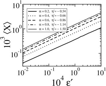
Figure 2: Average of $X$ from the map in equation (1), with the modulo $1$ reinjection and calculated with $10^{6}$ iterates at each of $10^{3}$ steps of the control parameter $\epsilon$. The log-log plot shows the same slope for all averages, independent of the value of $\alpha$ and $\eta^{\prime}$.

The same slope is obtained for the averages with different values of $\alpha$ and $\eta^{\prime}$. The resulting averages have the same dependence in $\epsilon$ as the one obtained from the map of second iterates (eq. (3)), calculated with the same number of iterates; all coinciding with the expression of eq. (6).

Figure 3 shows numerically calculated averages obtained directly from iterates of the map eq. (3), when $z=3$ and $z=7$. Again the initial condition at each value of $\epsilon$ was taken at random. A transient of $10^{5}$ iterates was eliminated from a total of $2\times 10^{7}$ calculated values at each of $10^{3}$ steps of $\epsilon$, between zero and $10^{-1}$.

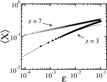
Figure 3: Average of $X$ from the map in equation (3), calculated with $2\times 10^{7}$ iterates at each of $10^{3}$ steps of the control parameter $\epsilon$. White squares are used for $z=7$ and filled circles for $z=3$. The thin lines correspond to the predicted values given by eqs. (6) and (7).

For $\epsilon<10^{-2}$ the $z=3$ and $7$ results are very well superimposed by the analytical curves made from equation (6), with $\nu=0.50$, and equation (7), with $\nu=1/6\approx 0.17$, respectively. The two behaviors are clearly distinguished in the log-log plot. For the purpose of comparison with the already established exponents one should notice that the exponents for the average laminar phase are given in kodama91 as $(z-2)/(z-1)$ that is $\beta=0.50$ and $\beta=0.83$, respectively, verifying $\nu+\beta=1$.

Up to this point all results have concerned discrete maps. Dynamical fluxes with associated maps having intermittent chaos show similar critical exponents for the average of its continuous variables. This has been verified numerically with tangent bifurcation of type-I intermittency hugomapaave2000 ; hugoave2000 and will be demonstrated here for a physical chaotic oscillator. For the type-III intermittency the map extracted from a flux has the form of eq. (3) for its second iterates. A discretely sampled continuous flux may be viewed as a finite set of discrete stroboscopic maps, all with the same stroboscopic frequency but stroboscopic phases ranging from 0 to $2\pi$ in uniformly separated steps. The number of such maps gives the ratio of sampling frequency to stroboscopic frequency. The time average of the continuous flux is the average of the time averages of these maps. If a map from this series is nonsymmetrical, only in very special cases it would happen that this asymmetry be exactly canceled by the summation on the other maps. Thus, in general, its expected that if the flux leads to a nonsymmetrical map (no odd symmetry with respect to the unstable fixed point) the average of its continuous variable will exhibit the same exponent $\nu$ of eq. (8).

IV Experimental exponents in a nonlinear circuit with intermittency

The physical experimental system to test the above exponents consisted of an RLC series circuit, where a nonlinear capacitance was implemented by a p-n junction diode testa82 ; buskirk85 . The circuit, presented in figure 4, was driven by a frequency and amplitude controllable oscillator with output impedance of $50$ Ohms. An inductor of $0.1$ Henry, an external resistor of $13$ Ohms and a (typical 1N4007) diode formed the circuit, whose linear oscillation regime had resonance frequency at $150$ kHz.

Figure 4: Experimental diagram of the RLD circuit showing type-III intermittent chaos. The voltage across the diode was the dynamical variable measured both in its peak value, to make maps, and integrated to give the averages. The circuit is drawn with thick lines, while thin lines are the high impedance probe and integrator.

Dynamical bifurcations were produced by scanning the external drive frequency. Time series of the value of the voltage across the diode and the current in the circuit were collect with a $12$ bits resolution converter. The sampling rate was $10^{7}$ sample/s. Thus $200$ points were saved on each oscillator cycle. Capturing $10^{4}$ points at each value of the control frequency, a simple software searched for the maxima in the series. In wide range scans the typical bifurcation diagrams given by the peak value of the voltage across the diode, show clearly the well known results of period doubling cascades, chaotic windows and tangent bifurcations from chaos into periodic windows. jeffries82 ; testa82 ; buskirk85 ; ono95 .

A specific bifurcation, with intermittency and no bistability, was found and studied, scanning the external oscillator frequency from $48708$ Hz to $48768$ Hz by $300$ equal small steps. The drive voltage amplitude was fixed at $2.7$ V. The circuit was mounted inside an isolating box to prevent thermal drift effects donoso97 . The value of a control parameter $\epsilon$ is obtained as the frequency detuning step divided by the critical frequency of the bifurcation, $48762$ Hz. Thus $\epsilon$ varied in the range of $10^{-4}$–$10^{-3}$. A segment of the voltage pulses is shown in figure 5. The signature of type-III intermittency is observed with the laminar events corresponding to the uniform oscillations alternating their peak value around 1V.

Figure 5: Voltage pulses measured across the diode in the RLD circuit. Successive maxima alternate their position respective to the $1$ V value until a chaotic burst occurs and reinjects back to the vicinity of the unstable orbit, typical of type-III intermittency

Multibranch maps constructed from the maxima of the voltage across the diode, extracted from series with $6\times 10^{5}$, could be approximated to one-dimensional ones, expected in the limit of infinite dissipation. Second return maps and laminar phase histograms, not shown here, indicate type-III intermittency. Figure 6 shows the average length of laminar phases for different values of $\epsilon$. Each histogram used was obtained with $6\times 10^{5}$ points. A theoretical fitting kodama91 is best with an exponent $\beta=0.62$. Notice that for the map the predictions are $\beta=0.5$ for $z=3$ and $\beta=0.75$ for $z=5$. However the experimental data always has excess of laminar events identified with short length griffith97 and this effect gives a bigger experimental value for $\beta$ in the fittings. Therefore, $z=3$ is the best odd value.The excess of short laminar phase events may be related to the finite dissipation rate in the phase space of the experimental system and the consequent non unidimensional maps and also to a nonuniform density of probability for the reinjection, as discussed by Kim et al. kim98 .

Figure 6: Measured average lengths of laminar oscillations in the driven circuit with a diode. The thick line is the theoretical fitting for type-III intermittency with exponent $\beta=0.62$

The peak value of the voltage, which gave the second return map and the histograms is shown in Figure 7(a). The laminar phases are the oscillations with repetitive visits to the maximum value near $1V$ in the figure. As the segments represented in figure 5(a) are short in time for many values of parameters they show a single laminar event with all points accumulated around the unstable orbit. Also shown is the simultaneously acquired average of the voltage across the diode. It was obtained with a simple electronic integrator, having a time constant of $3$ seconds. To account for long laminar phase events and (which is equivalent) decrease the average fluctuations the scan lasted 50 minutes.

Figure 7: (a) Peak voltage across the diode in the type-III bifurcation of the circuit. (b) Simultaneously measured average voltage. The thick line is a fitting of eq. (6) with exponent $\nu=0.55$

The experimental average voltage was fitted to the expression

$$\left<X(\epsilon)\right>=-{\epsilon}^{\nu}\ln{\epsilon}$$ (9)

The exponent $\nu=0.55$ gave an excellent agreement with the experimental plot, as shown in figure 7. Attempts of fittings to higher values of $z$, i.e., to eq. (7), failed. It is worth noticing that the value predicted for $z=5$ is $\nu=0.25$. Thus, the experimental average consistently verifies $z=3$ for the nonlinearity of this bifurcation in the circuit. The confidence for the experimental values of $\beta$ and $\nu$ from fittings using standard $\chi^{2}$ procedure is better than 2%. Therefore, the result $\beta+\nu=1.17\pm 0.02$ shows that a discrepancy remains between the experiments and the unidimensional map model. While the bigger value obtained for $\beta$ has been attributed to an excess of short laminar phase events kim98 no such study of deviations exists for the exponent in the averages.

V Conclusion

In conclusion, critical exponents for the averages of one dynamical variable are established analytically for type-III intermittent chaotic maps. Those exponents are directly related to the nonlinear power law of the normal form of the maps. They have a simple relation with the exponents of the average length of laminar iterates in the same systems. All these properties were verified in numerical experiments with maps.

Physical experiments with a continuous flux were also done to demonstrate the exponents in averages. The average voltage across a diode in a chaotic electronic circuit was measured while the drive frequency was scanned through bifurcations. A bifurcation from chaos into periodic pulsation, shown to be type-III intermittent, gives an exponent in agreement with the cubic nonlinearity. This result is consistently verified in the exponents of the average length of laminar phases, extracted from histograms of the peak pulse voltages in the circuit.

Averages of dynamical variables have been proposed to get the signature of the Lorenz chaos bifurcation lawandy87 , have been numerically studied in critical bifurcations rajasekar00 , and experimentally measured in bifurcating pulsed lasers oliveira96 . However no systematic study of critical exponents have been done.

The technique of measuring averages of dynamical variable in intermittent chaos is a complementary procedure to investigate bifurcations of nonlinear systems. The experimental average may also be advantageous when detection noise for an specific variable has a bandwidth overlapping the frequency bandwidth of the chaotic oscillations. For systems with high frequency noise it is naturally bound to be more sensitive. Its experimental motivation is therefore enhanced to characterize ultrafast chaotic oscillators, like diode lasers, using slow time detection techniques. One extension relevant to the work presented here is the study of the exponents for the averages in bifurcations with nonuniform reinjection in the intermittency, as studied by Kim et al. kim98 . A relation between exponents of the averages and the exponents of the average length of laminar phases events should exist generalizing the $\nu+\beta=1$ given here. Another potential use for the averages near bifurcation would be to complement the confrontation between experimental data and model as extracted from nonlinear data analysis hegger98 ; timmer2000 . The models inferred from the data analysis must have bifurcations consistent with the experimental system. These bifurcations could be tested comparing both the exponents of laminar events and the exponents of averages of dynamical variables. The Critical exponents have been introduced for many types of bifurcations in chaotic systems grebogi86 . Their presence in simple, experimentally accessible, statistical properties, as the averages and its higher moments, are under investigation. The earliest citation of averages in chaos can be traced to the original propositions of unpredictability in deterministic chaos lorenz64 .

References

- (1) Y. Pomeau, P. Manneville, Commun. Math. Phys. 74, 189, (1980)
- (2) P. Bergé, Y. Pomeau, Ch. Vidal, L’Ordre dans le Chaos, Paris: Hermann (1984) pp. 266-278.
- (3) P. Manneville, Dissipative Structures and Weak Turbulence, Academic Press, Boston, (1990) p. 129
- (4) C.-M. Kim, G.-S. Yim, J.-W. Ryu, Y.-J. Park, Phys. Rev. Lett. 80, 5317, (1998)
- (5) C. Jeffries and J. Perez, Phys. Rev. A 26, 2117, (1982)
- (6) K. Fukushima and T. Yamada, Journal Phys. Soc. Japan, 57 4055, (1988)
- (7) Y. Ono, K. Fukushima, and T. Yazaki, Phys. Rev. E 52, 4520, (1995)
- (8) D. Y. Tang, J. Pujol, and C. O. Weiss, Phys. Rev. A 44, R35, (1991)
- (9) T. M. Griffith, D. Parthimos, J. Crombie, and D. H. Edwards, Phys. Rev. E 56, R6287, (1997)
- (10) H. Kodama, S. Sato, and K. Honda, Phys. Lett. A 157, 354, (1991)
- (11) P. S. Linsay, Phys. Rev. Lett. 47, 1349, (1981)
- (12) J. Testa, J. Pérez, and C. Jeffries, Phys Rev. Lett. 48, 714, (1982)
- (13) R. Van Buskirk and C. Jeffries, Phys. Rev. A 31 3332, (1985)
- (14) See ref. 3 p. 264
- (15) H. L. D. de S. Cavalcante J. R. Rios Leite, Unpublished
- (16) A. Donoso, E. Machado, D. Valdivia, C. Fehr, and G. Gutierrez, Phys. Lett. A , 225, 79-84, (1997)
- (17) Hugo L. D. de S. Cavalcante and J. R. Rios Leite, Dynamics and Stabil. of Systems, 15, 35, (2000)
- (18) Hugo L. D. de S. Cavalcante and J. R. Rios Leite, Physica A 283, 125, (2000)
- (19) N. M. Lawandy, M. D. Selker, K. Lee, Opt. Commun. 61, 134, (1987)
- (20) S. Rajasekar, V. Chinnathambi, Chaos, Sol. and Fractals, 11, 859, (2000)
- (21) L. de B. Oliveira-Neto, G. J. F. T. da Silva, A. Z. Khoury, and J. R. Rios Leite, Phys. Rev. A 54, 3405, (1996)
- (22) R. Hegger, H. Kantz and F. Schmuser, Chaos 8, 727 (1998)
- (23) J. Timmer, H. Rust, W. Hobelt, and H. U. Voss, Phys. Lett. A, 274, (2000)
- (24) C. Grebogi, E. Ott, and J. A. Yorke Phys. Rev. Lett. 57, 1284, (1986)
- (25) E. N. Lorenz, Tellus, XVI, 1, (1964)