Spectral form factor of hyperbolic systems: leading off-diagonal approximation

Abstract

The spectral fluctuations of a quantum Hamiltonian system with time-reversal symmetry are studied in the semiclassical limit by using periodic-orbit theory. It is found that, if long periodic orbits are hyperbolic and uniformly distributed in phase space, the spectral form factor $K(\tau)$ agrees with the GOE prediction of random-matrix theory up to second order included in the time $\tau$ measured in units of the Heisenberg time (leading off-diagonal approximation). Our approach is based on the mechanism of periodic-orbit correlations discovered recently by Sieber and Richter [1]. By reformulating the theory of these authors in phase space, their result on the free motion on a Riemann surface with constant negative curvature is extended to general Hamiltonian hyperbolic systems with two degrees of freedom.

PACS numbers: 05.45.Mt, 03.65.Sq

1 Introduction

One of the fundamental characteristics of quantum systems with classical chaotic dynamics is the universality of their spectral fluctuations. This universality and the agreement with the predictions of random-matrix theory (RMT) was first conjectured by Bohigas, Giannoni and Schmit (BGS) [2]. It has been later supported by numerical investigations on a great variety of systems [3]. However, the necessary and sufficient conditions on the underlying classical dynamics leading to such a universality in quantum spectral statistics are not known, and the origin of the success of RMT in clean chaotic systems is still subject to debate.

In the semiclassical limit, where the BGS conjecture is expected to be valid, the Gutzwiller trace formula [4] expresses the density of states $\rho(E)=\sum_{n}\delta(E-E_{n})$ of the quantum system as a sum of a smooth part $\overline{\rho}(E)$ and an oscillating part. The latter is given by a sum ${\rho}_{\text{osc}}(E)=(\pi\hbar)^{-1}\sum_{\gamma}A_{\gamma}\,\cos(S_{\gamma}/\hbar-\pi\mu_{\gamma}/2)$ over all classical periodic orbits $\gamma$ of energy $E$ ($S_{\gamma}$ and $\mu_{\gamma}$ are the action and the Maslov index of $\gamma$, and $A_{\gamma}$ is an associated amplitude). The energy correlation function,

$$R(\epsilon)=\frac{1}{\overline{\rho}(E)^{2}}\left\langle\rho\left(E+\frac{\epsilon}{2}\right)\rho\left(E-\frac{\epsilon}{2}\right)\right\rangle_{E}-1\;,$$ (1)

and its Fourier transform $K(\tau)$, the so-called form factor, are given by sums over pairs $(\gamma,\gamma^{\prime})$ of periodic orbits. Here $\tau$ is the time measured in units of the Heisenberg time $T_{H}=2\pi\hbar\,\overline{\rho}(E)$ ($T_{H}={\mathcal{O}}(\hbar^{1-f})$ for systems with $f$ degrees of freedom). The brackets denote an (e.g. Gaussian) energy average over an energy width $W$ much larger than the mean level spacing $\Delta E=\overline{\rho}(E)^{-1}$, but classically small, $W\ll E$, so that $\langle\rho\rangle_{E}\simeq\overline{\rho}(E)$. By neglecting the ‘off-diagonal’ terms, i.e., the contributions of pairs of distinct orbits modulo symmetries, Berry [5] showed that the spectral fluctuations of classically chaotic systems agree in the limit $\hbar\rightarrow 0$ with the RMT predictions to first order in $\tau$ ($\tau\ll 1$). Two different approaches have been proposed to support the BGS conjecture to all orders in $\tau$ in the semiclassical limit. The first one is based on a mapping between the parameter level dynamics and the dynamics of a gas of fictitious particles [3, 6]. The second one uses field-theoretic and supersymmetric methods and applies to systems with exponential decays of classical correlation functions [7].

The link between spectral correlations and correlations among periodic orbits was first put forward in [8]. It was argued in this reference that the BGS conjecture implies some universality at the level of classical action correlations. Recently, Sieber and Richter [1] identified a general mechanism leading to correlations among periodic orbits in chaotic systems with two degrees of freedom having a time-reversal invariant dynamics. This has opened the route towards an understanding of the universality of spectral fluctuations based on periodic-orbit theory only. The crucial fact is that an orbit $\gamma$ having a self-intersection in configuration space with nearly antiparallel velocities is correlated with another orbit $\tilde{\gamma}$, having an avoided intersection instead of a self-intersection, which has almost the same action and amplitude. In two special systems, the free motion on a Riemann surface with constant negative curvature (Hadamard-Gutzwiller model) [1] and quantum graphs [9], the pairs $(\gamma,\tilde{\gamma})$ have been found to give a contribution $K_{2}(\tau)=-2\tau^{2}$ to the semiclassical form factor. This result is in agreement with the Gaussian orthogonal ensemble (GOE) prediction of RMT,

$$K_{\text{GOE}}(\tau) = 2\tau-\tau\ln(1+2\tau)\;\;\;,\;\;\;0<\tau<1$$ (2)

$$= 2\tau-2\tau^{2}+{\mathcal{O}}(\tau^{3})\;.$$

The first term $K_{1}(\tau)=2\tau$ is obtained by using Berry’s diagonal approximation.

The purpose of this work is to extend Sieber and Richter’s result to general hyperbolic and ergodic two-dimensional Hamiltonian systems. Unlike in [1], our approach does not rely on the concepts of self-intersections and avoided intersections with nearly antiparallel velocities, but rather focus on what corresponds to such events in phase space, namely the existence of two stretches of the orbit (for both $\gamma$ and $\tilde{\gamma}$) which are almost time reverse of one another. It will be argued that working in phase space has a number of advantages and may allow for easier generalisations to periodically driven systems and to systems with $f>2$ degrees of freedom. A similar approach is presented in [10]; an alternative approach, based on a projection onto the configuration space as in [1], is presented in [11].

In section 2, we state the main hypothesis on the classical dynamics used throughout this paper. After having briefly recalled the main ingredients of the theory of Sieber and Richter in section 3, a characterisation of the orbit pairs $(\gamma,\tilde{\gamma})$ in the Poincaré surface of section is given in section 4. The unstable and stable coordinates associated with a pair $(\gamma,\tilde{\gamma})$ are introduced in the following section. The leading off-diagonal correction $K_{2}(\tau)=-2\tau^{2}$ to the semiclassical form factor is derived in section 6. Our conclusions are drawn in the last section. Some technical details are presented in two appendixes.

2 Hyperbolic Hamiltonian systems

We consider a particle moving in a Euclidean plane ($f=$ two degrees of freedom), with Hamiltonian $H(\mbox{\boldmath{$q$}},\mbox{\boldmath{$p$}})=H(\mbox{\boldmath{$q$}},-\mbox{\boldmath{$p$}})$ invariant under time-reversal symmetry. We assume the existence of a compact two-dimensional Poincaré surface of section $\Sigma$ in the (four-dimensional) phase space $\Gamma$, contained in an energy shell $H(\mbox{\boldmath{$q$}},\mbox{\boldmath{$p$}})=E$ and invariant under time reversal (TR) [4, 12]. Every classical orbit of energy $E$ intersects $\Sigma$ transversally. The classical dynamics can then be described by an area-preserving map $\phi$ on $\Sigma$, together with a first-return time map $x\in\Sigma\mapsto t_{x}\in[0,\infty]$ (see [12]). In what follows, letters in normal and bold fonts are assigned to the canonical coordinates $x=(q,p)$ in $\Sigma$ and to points $\mbox{\boldmath{$x$}}=(\mbox{\boldmath{$q$}},\mbox{\boldmath{$p$}})$ in $\Gamma$, respectively. It is convenient to use dimensionless $q$ and $p$ by measuring them in units of some reference length $L$ and momentum $P$. The $n$-fold iterates of $x$ by the map are denoted by $x_{n}=\phi^{n}\,x$, $n\in{\mathbb{Z}}$. They are the coordinates of the intersection points $\mbox{\boldmath{$x$}}_{n}$ of a phase-space trajectory with $\Sigma$, according to a given direction of traversal. The Euclidean distance between two points of coordinates $x$ and $y$ in $\Sigma$ is denoted by $|y-x|$. If the system is a billiard ($H(\mbox{\boldmath{$q$}},\mbox{\boldmath{$p$}})=\mbox{\boldmath{$p$}}^{2}/2M$ if $q$ is inside a compact domain $\Omega\subset{\mathbb{R}}^{2}$ and $+\infty$ otherwise), $\Sigma$ is the set of points $(\mbox{\boldmath{$q$}},\mbox{\boldmath{$p$}})\in\Gamma$ such that $q$ is on the boundary $\partial\Omega$ of the billiard, $p$ is the momentum after the reflection on $\partial\Omega$, and $|\mbox{\boldmath{$p$}}|=\sqrt{2ME}$. Then $q$ is the arc length along $\partial\Omega$ in units of the perimeter $L$, $p$ is the momentum tangential to $\partial\Omega$ in units of $\sqrt{2ME}$, and $t_{x}$ is the length of the segment of straight line linking two consecutive reflection points, multiplied by the inverse velocity $\sqrt{M/2E}$ (see Fig. 1). Due to the Hamiltonian nature of the dynamics, the linearised $n$-fold iterated map $M_{x}^{(n)}=D_{x}(\phi^{n})$ is symplectic. This means that it conserves the symplectic product

$$\Delta x\wedge\Delta x^{\prime}=\Delta p\,\Delta q^{\prime}-\Delta q\,\Delta p^{\prime}$$ (3)

for any two infinitesimal displacements $\Delta x=(\Delta q,\Delta p)$ and $\Delta x^{\prime}=(\Delta q^{\prime},\Delta p^{\prime})$ in the tangent space ${\mathcal{T}}_{x}\Sigma$.

The time reversal (TR) acts in the phase space $\Gamma$ by changing the sign of the momentum, $T_{\Gamma}:(\mbox{\boldmath{$q$}},\mbox{\boldmath{$p$}})\mapsto(\mbox{\boldmath{$q$}},-\mbox{\boldmath{$p$}})$. Its action on $x$ is given by an area-preserving self-inverse map $T$. When acting on an infinitesimal displacement $\Delta x$ in ${\mathcal{T}}_{x}\Sigma$, the same symbol $T$ refers to the linearised version of $T$ (we avoid the cumbersome notation $D_{x}T$, the meaning of $T$ being clear from the context). In most cases, the exact map $T$ is already linear and given by $T:(q,p)\mapsto(q,-p)$. The TR symmetry of the Hamiltonian implies $\phi\,T=T\,\phi^{-1}$, i.e., $(Tx)_{n}=Tx_{-n}$.

Some spatially symmetric systems in an external magnetic field have non-conventional TR symmetries, obtained by composing $T_{\Gamma}$ with a canonical transformation associated with the spatial symmetry [3]. The Sieber-Richter pairs $(\gamma,\tilde{\gamma})$ of correlated orbits also exist in such systems, although they look different in configuration space [13]. By performing the canonical transformation to redefine new coordinates $(\mbox{\boldmath{$q$}},\mbox{\boldmath{$p$}})$ at the beginning, the TR becomes the conventional one. Therefore the analysis below also applies to systems with non-conventional TR symmetries.

The normalised $\phi$-invariant measure is the Liouville measure ${\rm{d}}\mu(q,p)={\rm{d}}q\,{\rm{d}}p/|\Sigma|$, where $|\Sigma|$ is the (dimensionless) area of $\Sigma$. Our main assumptions on the dynamical system $(\phi,\Sigma,\mu)$ are

• $\mu$ is ergodic;

• all Lyapunov exponents are different from zero on a set of points $x$ of measure one (complete hyperbolicity);

• long periodic orbits are ‘uniformly distributed in $\Sigma$’.

Note that (i) and (ii) imply that the Lyapunov exponents $\pm\lambda_{x}$ are constant $\mu$-almost everywhere and equal to $\pm\langle\lambda\rangle$, with $\langle\lambda\rangle>0$ (the periodic points are notable exceptions of measure zero where this is wrong!). Examples of billiards satisfying (i-ii) are semi-dispersing billiards (if trajectories reflecting solely on the neutral part of $\partial\Omega$ form a set of measure zero), the stadium and other Bunimovich billiards, the cardioid billiard, and the periodic Lorentz gas (see e.g. [14] and references therein). Assumption (iii), associated with ergodicity (i), means that an (appropriately weighted) average over periodic orbits with periods inside a given time window $[T,T+\delta T]$ can be replaced in the large-$T$ limit by a phase-space average [15, 16]. Note that this statement, which is the precise content of (iii), does not concern individual periodic orbits but rather averages over many periodic orbits with large periods. We think that the statement can hold true even if some periodic orbits with arbitrary large periods are stable, if there are exponentially less such orbits than unstable orbits.

As is typically the case in billiards, the Poincaré map $\phi$ or its derivatives may be singular on a closed set ${\mathcal{S}}\subset\Sigma$ of measure zero. For instance, if the boundary $\partial\Omega$ is concave outward, $\phi$ is discontinuous at a point $x_{S}=(q_{S},p_{S})$ such that the trajectory between $\mbox{\boldmath{$q$}}_{S}$ and the next reflection point is tangent to $\partial\Omega$ at this point (see Fig. 1). Let us denote by $d(x,{\mathcal{S}})$ the Euclidean distance from $x$ to ${\mathcal{S}}$. We assume that

• ${\mathcal{S}}$ is ‘not too big’: $\mu(B_{\delta,S})\leq C_{1}\,\delta^{\sigma_{1}}$ for any $\delta>0$, with $B_{\delta,S}=\{x\in\Sigma;|x-x_{S}|\leq\delta,x_{S}\in{\mathcal{S}}\}$ and $\sigma_{1}>0$;

• the divergence of the derivatives of $\phi$ on ${\mathcal{S}}$ is at most algebraic, $|\partial^{r}\phi/\partial x^{\alpha_{1}}\ldots\partial x^{\alpha_{r}}|\leq C_{2}\,d(x,{\mathcal{S}})^{-\sigma_{2}(r-1)}$, with $\sigma_{2}>0$.

Here $C_{1}>0$ and $C_{2}\geq 1$ are constants of order one and the indices $\alpha,\beta=1,2$ refer to the $q$- and $p$-coordinates in $\Sigma$ ($x^{1}=q$, $x^{2}=p$). (iv-v) are standard mathematical assumptions on billiard maps [17].

Figure 1: Billiard $\Omega$: $q_{n}$ and $p_{n}=\sin\beta_{n}$ are the arc length along $\partial\Omega$ and the momentum tangential to $\partial\Omega$ in dimensionless units.

3 The theory of Sieber and Richter

The starting point of Sieber and Richter is the semi-classical expression of the form factor,

$$K_{\text{semicl}}\left(\tau=\frac{T}{T_{H}}\right)=\frac{1}{T_{H}}\,\frac{1}{\delta T}\left\langle\;\sum_{T\leq(T_{\gamma}+T_{\gamma^{\prime}})/2\leq T+\delta T}A_{\gamma}A_{\gamma^{\prime}}\,e^{\frac{{i}}{\hbar}(S_{\gamma}-S_{\gamma^{\prime}})-{i}\frac{\pi}{2}(\mu_{\gamma}-\mu_{\gamma^{\prime}})}\right\rangle_{E}\;.$$ (4)

The sum runs over all pairs of periodic orbits $(\gamma,\gamma^{\prime})$ such that the half-sum of their periods $(T_{\gamma}+T_{\gamma^{\prime}})/2$ is in the time window $[T,T+\delta T]$ of width $\delta T\ll T_{H}$. For isolated periodic orbits, $A_{\gamma}=T_{\gamma}\,r_{\gamma}^{-1}|\det(M_{\gamma}^{(F)}-1)|^{-1/2}$, where $r_{\gamma}$ is the repetition (number of traversals) of $\gamma$ and $M_{\gamma}^{(F)}$ is the stability matrix of $\gamma$ for displacements perpendicular to the motion [4]. In order to work with a self-averaging form factor [18], a time averaging over the window $[T,T+\delta T]$ (with, e.g., $\delta T=h/W$) has been performed in (4). Equivalently, $K(\tau)$ can be defined as the truncated Fourier transform

$$K(\tau)=\overline{\rho}(E)\int_{-\infty}^{\infty}{\rm{d}}\epsilon\,R(\epsilon)\,\frac{\sin\left(\epsilon\,\delta T/2\hbar\right)}{\epsilon\,\delta T/2\hbar}\,e^{-\frac{{i}}{\hbar}\epsilon T}$$ (5)

of the energy correlation function (1). Formula (4) gives the correct form factor for small enough times $\tau$ only. It relates the quantum energy correlations to the classical action correlations [8]. Indeed, only orbits with correlated actions, differing by an amount of order $\hbar$, can interfere constructively in (4).

For fixed $\tau=T/T_{H}>0$, the sum (4) deals with orbits with very long periods as $\hbar\rightarrow 0$ (recall that $T_{H}={\mathcal{O}}(\hbar^{-1})$). Such orbits have many self-intersections in $q$-space, some of them characterised by small angles $\varepsilon$ at the crossing point. As shown in [1], the two loops at both sides of the crossing point can be slightly deformed in such a way that they form a neighbouring closed orbit in $q$-space, having an avoided crossing instead of a crossing (see Fig. 2). The two partner orbits $\gamma$ and $\tilde{\gamma}$ are almost time reverse of each other on one loop (right loop) and almost coincide on the other (left loop). Such a construction, which was supported in [1] by using the linearised dynamics, is in general possible in systems with TR symmetry and for small enough $\varepsilon$ only. Due to the hyperbolicity of $\gamma$, the two orbits come exponentially close to each other in $q$-space as one moves away from the crossing point $\mbox{\boldmath{$q$}}_{c}$. This means that the phase-space displacement perpendicular to the motion associated with $\gamma$ and $\tilde{\gamma}$ is almost (but not exactly) on the unstable manifold of $\gamma$ at $\mbox{\boldmath{$x$}}_{i,c}=(\mbox{\boldmath{$q$}}_{c},\mbox{\boldmath{$p$}}_{c,i})$, whereas the displacement associated with $\gamma$ and the TR of $\tilde{\gamma}$ is almost on the stable manifold of $\gamma$ at $\mbox{\boldmath{$x$}}_{i,c}$ [13]. If a symbolic dynamics is available, the symbol sequence of $\tilde{\gamma}$ can be constructed from the symbol sequence of $\gamma$ in a simple way [19]; in the Markovian case, the TR symmetry implies that the partner sequence must not be pruned. Since the two orbits $\gamma$ and $\tilde{\gamma}$ have almost the same period and almost the same Lyapunov exponents, the amplitudes $A_{\gamma}$ and $A_{\tilde{\gamma}}$ are almost equal. Furthermore, it can be shown by using a winding number argument that $\mu_{\tilde{\gamma}}=\mu_{\gamma}$ [10, 11]. In the Hadamard-Gutzwiller model, the difference $\delta S$ of the actions of $\tilde{\gamma}$ and $\gamma$ is given by $\delta S\simeq E\,\varepsilon^{2}/\lambda^{(F)}$ in the small $\varepsilon$ limit, where $\lambda^{(F)}$ is the positive Lyapunov exponent of the Hamiltonian flow [1]. The main hypothesis of [1] is that, if the system has no other symmetries than TR, only the pairs $(\gamma,\tilde{\gamma})$ contribute to the leading off-diagonal correction $K_{2}(\tau)$ to the semiclassical form factor (4) in the limit $\hbar\rightarrow 0$,

$$K_{2}(\tau)=\frac{1}{T_{H}}\,\frac{1}{\delta T}\left\langle\;\sum_{T\leq T_{\gamma}\leq T+\delta T}A_{\gamma}^{2}\,\sum_{\text{$\tilde{\gamma}$ partner of $\gamma$}}e^{\frac{{i}}{\hbar}\,\delta S}\right\rangle_{E}\;.$$ (6)

The main task is to evaluate the right-hand side. This was performed up to now for the Hadamard-Gutzwiller model [1] and for quantum graphs [9]. The main difficulties arising in extending the theory of Sieber and Richter to other systems satisfying the hypothesis in the previous section are

• the orbit $\gamma$ may have a family of correlated self-intersections, corresponding to one and the same partner orbit $\tilde{\gamma}$; this happens for instance in focusing billiards [11, 20]; care must be taken to avoid overcounting the pairs $(\gamma,\tilde{\gamma})$;

• the specific property of the Hadamard-Gutzwiller model is that all orbits $\gamma$ have the same positive Lyapunov exponent $\lambda^{(F)}$; this clearly does not hold in generic systems; then the action difference $\delta S$ expressed in terms of $\varepsilon$ depends in general on $\gamma$;

• the singularities $x_{S}\in{\mathcal{S}}$ of the map $\phi$ affect the number of self-intersections with small crossing angles $\varepsilon$ and may even ‘destroy’ the partner orbit $\tilde{\gamma}$ if $\gamma$ approaches ${\mathcal{S}}$ too closely.

We shall see in the following sections that working in the Poincaré surface of section enables one to resolve all these difficulties.

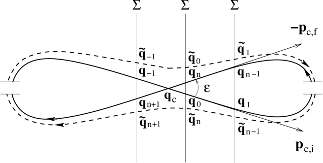
Figure 2: Pairs of correlated periodic orbits $\gamma$ (solid line) and $\tilde{\gamma}$ (dashed line) in configuration space for systems with conventional TR symmetry. The intersections of $q$-space with $\Sigma$ are schematically represented by parallel vertical lines.

4 The phase-space approach

4.1 Orbits with two almost time-reverse parts

As noted in [13], if an orbit $\gamma$ has a self-intersection at $\mbox{\boldmath{$q$}}_{c}$ with a small crossing angle $\varepsilon$ in configuration space, there are two phase-space points $\mbox{\boldmath{$x$}}_{c,i}=(\mbox{\boldmath{$q$}}_{c},\mbox{\boldmath{$p$}}_{c,i})$ and $\mbox{\boldmath{$x$}}_{c,f}=(\mbox{\boldmath{$q$}}_{c},\mbox{\boldmath{$p$}}_{c,f})$ on $\gamma$ which are nearly TR of one another, $\mbox{\boldmath{$x$}}_{c,i}\simeq T_{\Gamma}\,\mbox{\boldmath{$x$}}_{c,f}$. Indeed, $|\mbox{\boldmath{$p$}}_{c,i}+\mbox{\boldmath{$p$}}_{c,f}|\simeq|\mbox{\boldmath{$p$}}_{c,i}||\varepsilon|$ is very small for $|\varepsilon|\ll 1$ (see Fig. 2). There is in fact a part of $\gamma$ centred on $\mbox{\boldmath{$x$}}_{c,i}$ almost coinciding with the TR of another part of $\gamma$, centred on $\mbox{\boldmath{$x$}}_{c,f}$. The smaller the distance between $T_{\Gamma}\,\mbox{\boldmath{$x$}}_{c,f}$ and $\mbox{\boldmath{$x$}}_{c,i}$, the longer are these parts of orbit. There is therefore a family of points $\mbox{\boldmath{$x$}}_{m}$ of intersection of $\gamma$ with the surface of section $\Sigma$, with coordinates $x_{m}=\phi^{m}x$ such that

$$Tx_{n-m}\approx x_{m}\;,\;m=0,\pm 1,\pm 2,\ldots$$ (7)

(see Fig. 3(a)). The integer $n$ is the time (for the map) separating the two centres $x=x_{0}$ and $x_{n}$ of the two almost TR parts of $\gamma$.

It turns out that the breaking of the linear approximation (LA) plays an essential role in the existence of a family $\{\mbox{\boldmath{$x$}}_{m}\}$ with property (7). Indeed, we will show that, if the orbit $\gamma$ is unstable and $n$ is large, the displacements

$$\Delta x_{m}=Tx_{n-m}-x_{m}$$ (8)

cannot be determined from $\Delta x=\Delta x_{0}$ by using the LA for $m\geq n/2$. In order to make quantitative statements, and with the aim of transforming (7) into a precise definition, we introduce a small real number $c_{x}^{(t)}$, depending on $x$ and on an integer $t$, the latter denoting the current time. Loosely speaking, $c_{x}^{(t)}$ is the phase-space scale at which deviations from the LA after $t$ iterations of a point $y$ near $x$ start becoming important. More precisely, this number is defined as the maximal distance $|y_{m}-x_{m}|$ between the $m$-fold iterates of $y$ and $x$, for an arbitrary $y\approx x$ and an arbitrary time $m$ between $0$ and $t$, such that the final displacement $y_{t}-x_{t}$ can be determined from the initial displacement $y-x$ by using the LA, $y_{t}-x_{t}\simeq M_{x}^{(t)}(y-x)$ (recall that $M_{x}^{(t)}$ is the linearised $t$-fold iterated map) . As the errors of the LA may accumulate at each iteration, the larger the time $t$, the smaller must be $c_{x}^{(t)}$. We shall see below that $c_{x}^{(t)}$ decreases to zero like $t^{-1}$ for large $t$ if the map $\phi$ is smooth. If $\phi$ is not smooth, a typical trajectory in $\Sigma$ approaches a singularity point $x_{S}$ of $\phi$ arbitrarily closely between times $0$ and $t$ as $t\rightarrow\infty$. As a result, $c_{x}^{(t)}$ decreases to zero faster than $t^{-1}$ at large $t$ ($c_{x}^{(t)}$ even vanishes if $x$ hits $x_{S}$ after $m\leq t$ iterations, but such $x$ form a set of measure zero).

We can now define the time $m_{0}$ of breakdown of the LA for the displacements (7) as the largest integer such that

$$|\Delta x_{m}|\leq c_{x}^{(m_{0})}\;\;,\;\;m=0,\ldots,m_{0}\;.$$ (9)

In other words, $m_{0}$ is equal to the largest integer $m$ such that $\Delta x_{m}\simeq M_{x}^{(m)}\Delta x$. Similarly, going backward in time, we denote by $m_{0}^{T}$ the largest integer $m$ such that $\Delta x_{-m}\simeq M_{x}^{(-m)}\Delta x$. In what follows, we say that the orbit $\gamma$ has two almost TR parts separated by $n$ whenever (9) holds true for a family $\{\mbox{\boldmath{$x$}}_{m}\}$ of points of intersection of $\gamma$ with $\Sigma$, where $\Delta x_{m}$ is defined by (8). The point $\mbox{\boldmath{$x$}}_{0}$ is chosen among $\{\mbox{\boldmath{$x$}}_{m}\}$ in such a way that $|\Delta x_{0}|$ is minimum for $m=0$. This condition fixes $n$. In order to simplify the notation, we shall drop the index $0$ for the coordinate $x_{0}$ of the centre point $\mbox{\boldmath{$x$}}_{0}$, writing $x=x_{0}$ and, similarly, $\Delta x=\Delta x_{0}$. Since we are interested in the limit $|\Delta x_{0}|\ll c_{x}^{(m_{0})}$, we always assume that $m_{0}$ and $m_{0}^{T}$ are large (but much smaller than the period of $\gamma$). If $\gamma$ is unstable, then $|\Delta x_{m}|\simeq|M_{x}^{(m)}\Delta x|$ and $|\Delta x_{-m}|\simeq|M_{x}^{(-m)}\Delta x|$ grow exponentially fast with $m$ for large $m$ with the same rate $\lambda_{\gamma}$, $\lambda_{\gamma}=\lambda_{x}>0$ being the positive Lyapunov exponent of $\gamma$ for the Poincaré map. Moreover, the components of $\Delta x$ in the stable and unstable directions are roughly the same, since, by assumption, $|\Delta x_{m}|$ is minimum for $m=0$. This implies that $m_{0}^{T}\approx m_{0}$.

Let us first assume that $n$ is large. The exponential growth of $|\Delta x_{m}|$ in the regime of validity $m\leq m_{0}$ of the LA has the following consequence. Let us look at the distance in configuration space in Fig. 2 between the point $\mbox{\boldmath{$q$}}_{m}$, moving on the lower branch of the right loop as one increases $m$ (starting at $m=0$), and its ‘symmetric point’ $\mbox{\boldmath{$q$}}_{n-m}$, moving backward in time on the upper branch of the same loop. After the time $m=n/2$, the two points on the lower and upper branches of the loop are exchanged. Thus, the distance between these two points cannot increase for $m\geq n/2$. In contrast, it must decrease exponentially as $m$ approaches $n$, and come back to its initial value $|\mbox{\boldmath{$q$}}_{n}-\mbox{\boldmath{$q$}}_{0}|$ for $m=n$. It follows that the LA must break down before $m=n/2$, i.e., one has $m_{0}\leq n/2$. A similar reasoning holds in phase space. We first note that the $(n-m)$-fold iterates of $Tx_{n}$ and $x$ are equal to $Tx_{m}$ and $x_{n-m}$, respectively. Thanks to (8), $\Delta x_{n-m}=-T\Delta x_{m}$ for any integer $m$. The equality $|\Delta x_{n-m}|=|T\Delta x_{m}|$ would be violated if $2m_{0}\geq n\gg 1$, in view of the exponential growth of $|\Delta x_{m}|$ predicted by the LA. As a result, for large $n$, the condition

$$n\geq 2m_{0}$$ (10)

must be fulfilled.

Another situation arises when $n$ is of order $1$, $n\ll m_{0}$. Then the above-mentioned arguments do not apply since, if $m$ is of order $1$, the unstable and stable components of $\Delta x_{m}$ are of the same order and $|\Delta x_{m}|$ does not necessarily increase with $m$. Since $|\mbox{\boldmath{$q$}}_{n-m}-\mbox{\boldmath{$q$}}_{m}|\leq|Tx_{n-m}-x_{m}|\ll 1$ for all times $m$ between $-m_{0}^{T}$ and $m_{0}\gg n$, the right loop in Fig. 2 consists of two almost parallel lines, connected by a small piece of line with length of order $\langle l\rangle$, $\langle l\rangle$ being the mean length of a trajectory between two consecutive intersections with $\Sigma$. This means that the orbit $\gamma$ has an almost self-retracing part in $q$-space, centred at $\mbox{\boldmath{$q$}}_{0}$.

To conclude, we have shown that $n_{0}=2m_{0}$ has the meaning of a minimal time separating two distinct almost TR parts of $\gamma$ (i.e., excluding almost self-retracing parts). A similar result is obtained in [10, 11] for continuous times. The continuous-time version of $n_{0}$ is the minimal time $T_{0}$ to close a loop in $q$-space introduced in [1]. In the present context, this time arises with the new interpretation of the breakdown of the LA.

Let $N$ be the period of $\gamma$ for the Poincaré map. If the family $\{\mbox{\boldmath{$x$}}_{m}\}$ fulfils condition (9), then the family of almost TR points $\{\mbox{\boldmath{$x$}}_{n+m}\}$ also fulfils this condition, with $n$ replaced by $N-n$. This expresses the fact that, for a periodic orbit, the existence of a right loop in $q$-space implies the existence of a left loop (Fig. 2). Setting $y=x_{n}$, one has $Ty_{N-n-m}-y_{m}=-T\Delta x_{-m}$ and thus $|Ty_{N-n-m}-y_{m}|\leq\|T\|\,c_{x}^{(-m_{0}^{T})}$ for $m=0,\ldots,m_{0}^{T}$. This indeed shows that if $\{\mbox{\boldmath{$x$}}_{m}\}$ satisfies (9), then this is also the case for $\{\mbox{\boldmath{$x$}}_{n+m}\}$ with $n$ replaced by $N-n$, $m_{0}$ by $m_{0}^{\prime}\approx m_{0}^{T}$, and $m_{0}^{T}$ by ${m_{0}^{T}}^{\prime}\approx m_{0}$.

The distinction made in the previous section between a self-intersecting orbit and an orbit with an avoided crossing in $q$-space is irrelevant in the surface of section $\Sigma$: both orbits have two parts which are almost TR of one another. In other words, they both have families of points $\{\mbox{\boldmath{$x$}}_{m}\}$ and $\{\mbox{\boldmath{$x$}}_{n+m}\}$ satisfying (9). Note that these two families can correspond in $q$-space with a family of self-intersections, as in the case of focusing billiards if self-intersections occur at conjugate points [11, 20], or with one self-intersection (or one avoided crossing) only, as in the case of the Hadamard-Gutzwiller model [1].

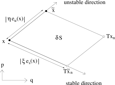
Figure 3: (a) The two families $\{x_{m}\}$ and $\{\tilde{x}_{m}\}$ in the surface of section $\Sigma$ (only few points are represented). (b) Magnification of (a) near $x=x_{0}$. The $N$-periodic points $x$, $\tilde{x}$, $Tx_{n}$, and $T\tilde{x}_{n}$ pertain to $\gamma$ (filled circles), $\tilde{\gamma}$ (filled squares), the TR of $\gamma$ (empty circles), and the TR of $\tilde{\gamma}$ (empty squares).

4.2 The partner orbit

We can now construct the partner orbit $\tilde{\gamma}$ described in section 3 in the surface of section $\Sigma$. Let $\gamma$ be an unstable orbit of period $N$ with two almost TR parts separated by $n<N$. The orbit $\tilde{\gamma}$ is defined by a $N$-periodic point $\tilde{x}=\tilde{x}_{0}$ lying close to $x=x_{0}$. This point is such that

$$\begin{cases}|T\tilde{x}_{n-t}-x_{t}|\ll 1&\text{for $t=0,\ldots,n$}\\ |\tilde{x}_{t}-x_{t}|\ll 1&\text{for $t=n,\ldots,N$.}\end{cases}$$ (11)

It can be checked in Fig. 2 that these properties indeed define the desired partner orbit. Note the symmetry of (11) with respect to the exchange of $x$ and $\tilde{x}$. By determining $\delta x=\tilde{x}-x$ as a power series in $\Delta x$, it is shown in appendix A that $x$ has at most one partner point $\tilde{x}$. These arguments indicate moreover that $\tilde{x}$ exists if $|\Delta x|$ is ‘sufficiently small’ and the two almost TR parts of $\gamma$ are sufficiently far apart from a singularity point of $\phi$. To first order in $\Delta x$, it is found in appendix A that

$$\delta x=\tilde{x}-x=T\bigl{(}1-M^{(n)}_{x}M^{(N-n)}_{Tx}\bigr{)}^{-1}\bigl{(}M^{(n)}_{x}+T\bigr{)}\Delta x$$ (12)

in agreement with [1]. The matrices $M_{x}^{(n)}$ and $M^{(N-n)}_{Tx}$ appearing in (12) are the stability matrices of the right loop and of the TR of the left loop in Fig. 2.

The partner point associated with $x_{m}$, $-m_{0}^{T}\leq m\leq m_{0}$, coincides with the $m$-fold iterate $\tilde{x}_{m}=\phi^{m}\tilde{x}$ of $\tilde{x}$. This can be seen by noting that $\tilde{x}_{m}$ satisfies (11) with $x$ replaced by $x_{m}$ and $n$ replaced by $n-2m$, as follows by combining (11) with (9). Hence, by uniqueness, $\tilde{x}_{m}$ is the partner point of $x_{m}$. It is not difficult to check this statement explicitly to lowest order in $\Delta x$ on (12) (see appendix A). We conclude that the partner points of all points $x_{m}$, $-m_{0}^{T}\leq m\leq m_{0}$, belong to the same orbit $\tilde{\gamma}$. In other words, if $|\Delta x|\ll 1$, there is a unique partner orbit $\tilde{\gamma}$ associated with the whole family $\{\mbox{\boldmath{$x$}}_{m}\}$. If this family is almost self-retracing, i.e., if $n\ll m_{0}$, this orbit coincides with $\gamma$ itself, as already noted elsewhere [20]. Actually, then $\tilde{x}=x$ satisfies (11), hence $\tilde{\gamma}=\gamma$ by uniqueness of the partner point (within the LA, this can be seen by replacing $T\Delta x=-\Delta x_{n}=-M_{x}^{(n)}\Delta x$ in (12); the identity $\Delta x_{n}=M_{x}^{(n)}\Delta x$ follows from $n\leq m_{0}$). By using a similar argument, one shows that the orbit $\tilde{\gamma}^{\prime}$ constructed from the family $\{\mbox{\boldmath{$x$}}_{n+m}\}$ is the TR of $\tilde{\gamma}$, as is immediately clear in Fig. 2.

4.3 A simple example: the baker’s map

The main advantage of the above-mentioned construction of the pairs $(\gamma,\tilde{\gamma})$ is that it works whatever the dimension of $\Sigma$ (i.e., for systems with $f>2$ degrees of freedom as well). Moreover, it applies to hyperbolic maps. It is instructive to exemplify this construction in the case of the baker’s map. Then $\Sigma$ is the unit square. It is convenient to equip $\Sigma$ with the distance $|x-x^{\prime}|=\max\{|q-q^{\prime}|,|p-p^{\prime}|\}$. A point $x=(q,p)\in\Sigma$ is in one-to-one correspondence with a bi-infinite sequence $\omega=\cdots\omega_{-2}\,\omega_{-1}\,.\,\omega_{0}\,\omega_{1}\,\omega_{2}\cdots$, obtained from the binary decompositions of $q$ and $p$ ($q=\sum_{l>0}\omega_{l-1}\,2^{-l}$ and $p=\sum_{l>0}\omega_{-l}\,2^{-l}$), with binary symbols $\omega_{l}\in\{0,1\}$, $l\in{\mathbb{Z}}$. The map $\phi$ acts on $\omega$ by shifting the point ‘.’ one symbol to the right. The TR symmetry is the reflection with respect to the diagonal of the square, $T:(q,p)\mapsto(p,q)$. This corresponds to reversing the order of the symbols of $\omega$, i.e., $T:\omega\mapsto\omega^{T}=\cdots\omega_{2}\,\omega_{1}\,\omega_{0}\,.\,\omega_{-1}\,\omega_{-2}\,\cdots$. Periodic points are associated with sequences $\omega$ containing a finite word $\omega_{0}\cdots\omega_{N-1}$, which repeats itself periodically; one usually writes the finite word only, keeping in mind that circular permutations of this word correspond to the same orbit. It is easy to see that the condition (9) with $c_{x}^{(m_{0})}=2^{-s}$ is satisfied if $\omega_{n-l-1}=\omega_{l}$ for any $l=-s,\ldots,m_{0}+s-1$. Similarly, the condition $|\Delta x_{-m}|\leq 2^{-s}$, $m=0,\ldots,m_{0}^{T}$, is satisfied if $\omega_{n-l-1}=\omega_{l}$ for any $l=-m_{0}^{T}-s,\ldots,s-1$. This means that $\omega$ has the form

$$x\;\;\longleftrightarrow\;\;\omega=Z^{T}_{L}\,L\,Z_{L}\,.\,Z_{R}\,R\,Z^{T}_{R}\;,$$ (13)

where $Z_{L}$, $Z_{R}$, $L$, and $R$ are finite words containing $(m_{0}^{T}+s)$, $(m_{0}+s)$, $(N-2m_{0}^{T}-2s)$, and $(n-2m_{0}-2s)$ symbols, respectively. The symbol sequence of the partner point $\tilde{x}$ is obtained by reversing time on $R$ and leaving all other symbols unchanged,

$$\tilde{x}\;\;\longleftrightarrow\;\;\tilde{\omega}=Z^{T}_{L}\,L\,Z_{L}\,.\,Z_{R}R^{T}Z^{T}_{R}\;.$$ (14)

The inequality $n>2m_{0}+2s$ must be fulfilled in order that $R$ is nonempty. In the opposite case, $\omega$ has an almost self-retracing part $Z_{L}Z_{R}Z^{T}_{R}Z^{T}_{L}$ and $\tilde{\omega}=\omega$. Similar pairs $(\omega,\tilde{\omega})$ of symbol sequences occur in the Hadamard-Gutzwiller model [19] and in certain billiards [20]. The families $\{x_{m}\}$ and $\{\tilde{x}_{m}\}$ look like those in Fig. 3(a) after a rotation by an angle $\pi/4$.

5 Use of the unstable and stable coordinates

To evaluate the leading off-diagonal correction $K_{2}(\tau)$ to the form factor, we shall first consider the second sum in (6) over all partner orbits $\tilde{\gamma}$ of $\gamma$, for a fixed unstable periodic orbit $\gamma$, which will be assumed to be infinitely long and to cover densely and uniformly the surface of section. We will then argue in section 6 that one can replace the obtained result inside the sum over $\gamma$ in the limit $T\rightarrow\infty$. The sum over the partner orbits $\tilde{\gamma}$ of $\gamma$ is to be expressed as an integral over some continuous parameters characterising $\tilde{\gamma}$, chosen such that the action difference $\delta S=S_{\tilde{\gamma}}-S_{\gamma}$ is a function of these parameters only. In configuration space, one may integrate over the crossing angle $\varepsilon$ [1]. It is argued in this section that a convenient choice of parameters in the surface of section is given by the unstable and stable coordinates of the small displacement $\Delta x$. The local coordinate system defined by the unstable and stable directions is singled out by the stretching and squeezing properties of the dynamics. These properties play a crucial role in the theory of Sieber and Richter, because they determine the time $m_{0}$ of breakdown of the LA and the exponential smallness of the distances (11).

5.1 The coordinate family ${\mathcal{L}}_{x,\eta,\xi}$

Under the hyperbolicity assumption (ii), there are at almost all $y\in\Sigma$ two vectors $e_{u}(y)$ and $e_{s}(y)$ tangent to the unstable and stable manifolds at $y$, which span the whole tangent space ${\mathcal{T}}_{y}\Sigma$. These vectors can be found by means of the cocycle decomposition [12],

$$M_{y}^{(m)}e_{u}(y)=\Lambda_{u,y}^{(m)}\,e_{u}(y_{m})\;\;\mbox{ , }\;\;M_{y}^{(m)}e_{s}(y)=\Lambda_{s,y}^{(m)}\,e_{s}(y_{m})\;,$$ (15)

where $\Lambda_{u,y}^{(m)}$ and $\Lambda_{s,y}^{(m)}$ are the stretching and squeezing factors. Because $M_{y}^{(m)}$ is symplectic, $\Lambda_{s,y}^{(m)}=1/\Lambda_{u,y}^{(m)}$ and the symplectic product $e_{u}(y)\wedge e_{s}(y)$ is independent of $y$ (see [12]). The vectors $e_{u,s}(y)$ can be ‘normalised’ in such a way that this constant is equal to $1$,

$$e_{u}(y)\wedge e_{s}(y)=1\;.$$ (16)

The product of the norms of $e_{u}(y_{m})$ and $e_{s}(y_{m})$ diverges as $m\rightarrow\pm\infty$ if the angle between the unstable and stable directions at $y_{m}$ decreases to zero. Since the exponential growth of $M_{y}^{(m)}e_{u}(y)$ at large $m$ is (by definition) captured by the stretching factor, the divergence of $|e_{u,s}(y_{m})|$ is smaller than exponential, $\ln|e_{u,s}(y_{m})|=o(m)$ [12]. The notation $f(m)=o(m)$, where $f$ is an arbitrary function over integers, stands for $f(m)/m\rightarrow 0$ as $m\rightarrow\pm\infty$. The stretching factor $\Lambda_{y}^{(m)}=\Lambda_{u,y}^{(m)}$ satisfy

$$\ln|\Lambda^{(m)}_{y}|=m\lambda_{y}+o(m)$$ (17)

where $\lambda_{y}$ is the positive Lyapunov exponent at $y$. If $y$ belongs to a periodic orbit $\gamma$ with period $N$, then $e_{u,s}(y)$ are the eigenvectors of the stability matrix $M_{y}^{(N)}$ of $\gamma$ and $|\Lambda_{y}^{(N)}|=\exp(N\lambda_{\gamma})$. By invoking the TR symmetry, $M_{Ty}^{(m)}T=TM_{y}^{(-m)}$. Replacing this expression into (15), one finds $e_{u,s}(Ty)\propto Te_{s,u}(y)$, with some $\phi$-invariant proportionality factors. By ergodicity, these factors are almost everywhere constant ($y$-independent). One can thus ‘normalise’ $e_{u,s}(Ty)$ in such a way that

$$e_{u}(Ty)=Te_{s}(y)\;\mbox{ , }\;e_{s}(Ty)=Te_{u}(y)\;\mbox{ , }\;\Lambda_{Ty}^{(m)}=\Lambda_{y_{-m}}^{(m)}$$ (18)

for almost all $y\in\Sigma$. Note that this agrees with (16), since $Te_{s}(y)\wedge Te_{u}(y)=e_{u}(y)\wedge e_{s}(y)$.

Two almost TR parts of an unstable orbit $\gamma$ can be parametrised by the family

$${\mathcal{L}}_{x,\eta,\xi}=\left\{(\eta_{m},\xi_{m})\,;\,-m_{0}^{T}\leq m\leq m_{0}\right\}\subset{\mathbb{R}}^{2}$$ (19)

of the unstable and stable coordinates $(\eta_{m},\xi_{m})$ of the displacements $\Delta x_{m}$,

$$\Delta x_{m}=Tx_{n-m}-x_{m}=\eta_{m}\,e_{u}(x_{m})+\xi_{m}\,e_{s}(x_{m})\;.$$ (20)

Thanks to (15),

$$\eta_{m}=\Lambda^{(m)}_{x}\,\eta\;\mbox{ , }\;\xi_{m}=\frac{\xi}{\Lambda^{(m)}_{x}}\;\mbox{ , }\;\eta_{m}\,\xi_{m}=\eta\,\xi\;,$$ (21)

where $-m_{0}^{T}\leq m\leq m_{0}$ and $\eta=\eta_{0}$, $\xi=\xi_{0}$. The points $(\eta_{m},\xi_{m})\in{\mathcal{L}}_{x,\eta,\xi}$ are located on a hyperbole in the $(\eta,\xi)$-plane (see Fig. 4).

In the case of the baker’s map (section 4.3), $e_{u}(y)$ and $e_{s}(y)$ are independent of $y$ and coincide with the unit vectors in the $q$- and $p$-directions. The stretching factors $\Lambda_{y}^{(m)}=2^{m}$ are also $y$-independent. The coordinates $\eta_{m}$ and $\xi_{m}$ are the usual $q$- and $p$-coordinates of $\Delta x_{m}=Tx_{n-m}-x_{m}$,

$$\left\{\begin{array}[]{ccccc}\eta_{m}&=&p_{n-m}-q_{m}&=&2^{m}(p_{n}-q)\\ \xi_{m}&=&q_{n-m}-p_{m}&=&2^{-m}(q_{n}-p)\,.\end{array}\right.$$ (22)

Figure 4: Domain ${\mathcal{D}}_{\gamma,a,\nu}$ in the $(\eta,\xi)$-plane (region marked by horizontal lines). The black points are the points $(\eta_{m},\xi_{m})$ in ${\mathcal{L}}_{x,\eta,\xi}$; $\nu$ of them are contained in ${\mathcal{D}}_{\gamma,a,\nu}$.

5.2 Estimation of $m_{0}$

In the limit $\eta,\xi\rightarrow 0$, the time $m_{0}$ of breakdown of the LA depends logarithmically on the unstable coordinate $\eta$,

$$m_{0}=-\frac{\ln|\eta|}{\lambda_{\gamma}}+o\left(\lambda_{\gamma}^{-1}\ln|\eta|\right)\;.$$ (23)

Indeed, thanks to hyperbolicity, $|\Delta x_{m}|$ grows exponentially fast with $m$ with the rate $\lambda_{\gamma}>0$, until it reaches, for $m=m_{0}$, a value of the order of the phase-space scale $c_{x}^{(m_{0})}$ at which deviations from the LA start becoming important. Since $|\Delta x_{m_{0}}|\approx|\eta_{m_{0}}|$, one must have $\ln(|\eta|/c_{x}^{(m_{0})})\sim-m_{0}\,\lambda_{\gamma}$. More precisely, we may approximate $|\Delta x_{m}|$ by $|\eta_{m}||e_{u}(x_{m})|$ for $m=m_{0}$ and $m=m_{0}+1$, making an exponentially small error for large $m_{0}$ (recall that $|\eta||e_{u}(x)|\approx|\xi||e_{s}(x)|$). By definition, $|\Delta x_{m_{0}}|$ is smaller than $c_{x}^{(m_{0})}$ and $|\Delta x_{m_{0}+1}|$ is greater than $c_{x}^{(m_{0}+1)}$. Then (23) follows from (17), (21), and $\ln|e_{u}(x_{m})|=o(m)$. Note that the terms $\lambda_{\gamma}^{-1}|\ln c_{x}^{(m_{0})}|$ and $\lambda_{\gamma}^{-1}|\ln c_{x}^{(m_{0}+1)}|$ have been neglected in (23). As stated in section 4.1, for a smooth map $\phi$, $c_{x}^{(m_{0})}$ decreases to zero like $m_{0}^{-1}$ as $m_{0}\rightarrow\infty$, i.e., as $\eta\rightarrow 0$. Therefore, $|\ln c_{x}^{(m_{0})}|$ is of order $\ln m_{0}={\mathcal{O}}(\ln|\ln|\eta||)$ and can be incorporated in the error term in (23). If $\phi$ has singularities on $\Sigma$, $c_{x}^{(m_{0})}$ decreases to zero faster than $m_{0}^{-1}$ as $\eta\rightarrow 0$. In such case, it will be argued in section 6.2 that formula (23) is not valid for all orbits $\gamma$. However, the right-hand side of (23) always gives an upper bound on $m_{0}$. Strictly speaking, the asymptotic behaviours (17) and (23) provide good approximations only if $m_{0}$ is close to a multiple of (or is much larger than) the period $N$ of $\gamma$. The physically relevant values of $m_{0}$ are, however, such that $1\ll m_{0}\ll N$. For such $m_{0}$’s, (23) should give nevertheless a reasonable approximation of the average value of $m_{0}$ (in fact it gives a good approximation of the inverse of the average of the inverse of $m_{0}$). This average can be taken over all points $x$ on $\gamma\cap\Sigma$ satisfying (9) such that the unstable and stable coordinates of $\Delta x=Tx_{n}-x$ are in small intervals $[\eta,\eta+{\rm{d}}\eta]$ and $[\xi,\xi+{\rm{d}}\xi]$, for an arbitrary integer $n\leq N/2$ and some fixed $\eta$, $\xi$, ${\rm{d}}\eta\ll|\eta|\ll 1$, and ${\rm{d}}\xi\ll|\xi|\ll 1$.

One shows similarly that

$$m_{0}^{T}=-\frac{\ln|\xi|}{\lambda_{\gamma}}+o(\lambda_{\gamma}^{-1}\ln|\xi|)\;.$$ (24)

For the baker’s map, in view of (22), $2^{m_{0}}|p_{n}-q|\leq 2^{-s}\leq 2^{m_{0}+1}|p_{n}-q|$, where we have chosen $c_{x}^{(m_{0})}=2^{-s}$. If $m_{0}\gg s$, this yields $m_{0}\simeq-\ln|p_{n}-q|/\ln 2$ and, similarly, $m_{0}^{T}\simeq-\ln|q_{n}-p|/\ln 2$, in agreement with (23) and (24).

5.3 The probability of ‘near-head-on return’

To count the number of partner orbits of an orbit $\gamma$ with a very large period $N$, one needs to know the probability to have two points on $\gamma$ which are nearly TR of one another. The aim of this subsection is to determine the (unnormalised) probability density $P_{\gamma}(\eta,\xi)$ associated with the unstable and stable coordinates of $\Delta x_{t}=Tx_{t+n}-x_{t}$, for all pairs $(\mbox{\boldmath{$x$}}_{t},\mbox{\boldmath{$x$}}_{t+n})$ of almost TR points on $\gamma\cap\Sigma$ which do not pertain to an almost self-retracing family (i.e., such that $n\geq 2m_{0}$). This density is defined through the number $P_{\gamma}(\eta,\xi)\,{\rm{d}}\eta\,{\rm{d}}\xi$ of points $\mbox{\boldmath{$x$}}_{t}$ on $\gamma\cap\Sigma$ such that the unstable and stable coordinates of $\Delta x_{t}$ are in the infinitesimal intervals $[\eta,\eta+{\rm{d}}\eta]$ and $[\xi,\xi+{\rm{d}}\xi]$, for an arbitrary integer $n$ between $2m_{0}(x_{t},\eta)$ and $N/2$. Let us recall that the partner orbits $\tilde{\gamma}$ and $\tilde{\gamma}^{\prime}$ built from the two families $\{\mbox{\boldmath{$x$}}_{m}\}$ and $\{\mbox{\boldmath{$x$}}_{n+m}\}$, separated from their almost TR families by the times $n$ and $N-n$, respectively, are TR of one another (section 4). The two pairs $(\gamma,\tilde{\gamma})$ and $(\gamma,\tilde{\gamma}^{\prime})$ have thus identical contributions to the form factor (6) (the corresponding action differences $\delta S$ are clearly the same). This is why it suffices to consider only the orbits $\tilde{\gamma}$ constructed from the family with the smaller time, $n\leq N/2$.

Let us define the infinitesimal parallelograms ${\rm{d}}\Sigma_{x,\eta,\xi}$ in $\Sigma$ by

$${\rm{d}}\Sigma_{x,\eta,\xi}=\Bigl{\{}y\in\Sigma\;;\;\eta\leq(y-x)_{u}\leq\eta+{\rm{d}}\eta\;,\;\xi\leq(y-x)_{s}\leq\xi+{\rm{d}}\xi\;\Bigr{\}}$$ (25)

where $(y-x)_{u,s}$ are the unstable and stable coordinates of $y-x$. Then

$${P}_{\gamma}(\eta,\xi)\,{\rm{d}}\eta\,{\rm{d}}\xi=\sum_{t=0}^{N-1}\sum_{n=2m_{0}(x_{t},\eta)}^{N/2}\chi\bigl{(}Tx_{n+t}\in{\rm{d}}\Sigma_{x_{t},\eta,\xi}\bigr{)}$$ (26)

where $\chi({\mathcal{P}})$ equals $1$ if the property ${\mathcal{P}}$ is true and $0$ otherwise. We shall assume here that the periodic orbit $\gamma$ covers densely and uniformly the surface of section $\Sigma$. If $N\gg 4m_{0}\gg 1$, the sum over $n$ can then be replaced by a phase-space integral, giving

$${P}_{\gamma}^{\,\text{erg}}(\eta,\xi)\,{\rm{d}}\eta\,{\rm{d}}\xi=\sum_{t=0}^{N-1}\left(\frac{N}{2}-2m_{0}(x_{t},\eta)\right)\int{\rm{d}}\mu(y)\,\chi\bigl{(}Ty\in{\rm{d}}\Sigma_{x_{t},\eta,\xi}\bigr{)}\;.$$ (27)

This integral is nothing but the area $|T{\rm{d}}\Sigma_{x_{t},\eta,\xi}|=|{\rm{d}}\Sigma_{x_{t},\eta,\xi}|$ of the parallelogram (25) per unit area. By (16), it is equal to ${\rm{d}}\eta\,{\rm{d}}\xi/|\Sigma|$. In virtue of (23),

$${P}_{\gamma}^{\,\text{erg}}(\eta,\xi)\simeq\frac{N}{2|\Sigma|}\left(N+\frac{4\,\ln|\eta|}{\lambda_{\gamma}}\right)\;.$$ (28)

It is worth noting that the ergodic hypothesis implies the identity between (26) and (27) for a set of points $x_{0}$ of measure one, and does not tell anything a priori about the points $x_{0}$ on periodic orbits, of measure zero in $\Sigma$. We shall argue below that, although (26) and (27) may differ for individual periodic orbits $\gamma$ which do not cover $\Sigma$ uniformly, one can use the ergodic result (28) to calculate the form factor in the semiclassical limit.

5.4 The domain ${\mathcal{D}}_{\gamma,a,\nu}$

The density $P_{\gamma}(\eta,\xi)$ just defined overcounts the number of partner orbits $\tilde{\gamma}$ relevant for the form factor. Actually, a unique partner orbit $\tilde{\gamma}$ is associated with each family $\{\mbox{\boldmath{$x$}}_{m};-m_{0}^{T}\leq m\leq m_{0}\}$ (section 4.2), whereas all points $\mbox{\boldmath{$x$}}_{m}$ belonging to the same family are counted separately in $P_{\gamma}(\eta,\xi)$. To avoid overcounting, we define a domain ${\mathcal{D}}_{\gamma,a,\nu}$ in the $(\eta,\xi)$-plane ${\mathbb{R}}^{2}$, having the good property to contain, for any $(\eta,\xi)$ inside this domain, a fixed number $\nu$ of elements $(\eta_{m},\xi_{m})$ in the family ${\mathcal{L}}_{x,\eta,\xi}$. This integer $\nu$ is independent of $\eta$ and $\xi$ (and thus of $m_{0}$ and $m_{0}^{T}$) and is such that $1\ll\nu\ll N$. Provided that this condition is fulfilled, the precise value of $\nu$ does not matter for the final result. Introducing also a small number $a>0$ controlling the maximal values of $|\eta|$ and $|\xi|$, we define

$${\mathcal{D}}_{\gamma,a,\nu}=\left\{(\eta,\xi)\in{\mathbb{R}}^{2}\mbox{ ; }e^{-\nu\lambda_{\gamma}}\leq\frac{|\xi|}{|\eta|}\leq e^{\nu\lambda_{\gamma}}\mbox{ , }|\eta\,\xi|\leq a^{2}\;\right\}\;.$$ (29)

If $(\eta,\xi)$ belongs to ${\mathcal{D}}_{\gamma,a,\nu}$, then $|\eta|$ and $|\xi|$ are bounded by $a\,e^{\nu\lambda_{\gamma}/2}$. The domain ${\mathcal{D}}_{\gamma,a,\nu}$ is represented in Fig. 4. For any $(\eta,\xi)\in{\mathcal{D}}_{\gamma,a,\nu}$, it contains $d_{x}\simeq\nu$ elements of the family ${\mathcal{L}}_{x,\eta,\xi}$. Actually, in view of (17) and (21),

$$\ln\left(\frac{|\xi_{m}|}{|\eta_{m}|}\right)=\ln\left(\frac{|\xi|}{|\eta|}\right)-2m\lambda_{\gamma}+o(m)\;\mbox{ , }\;1\ll|m|\leq\min\{m_{0},m_{0}^{T}\}\;.$$ (30)

By choosing $a$ small enough, one has, thanks to (23), $m_{0}+o(m_{0})\geq\nu$ for any $(\eta,\xi)\in{\mathcal{D}}_{\gamma,a,\nu}$ (for instance, if $c_{x}^{(m_{0})}=b\,m_{0}^{-\alpha}$ with $b,\alpha>0$, one may choose $a=b\,e^{-3\nu\lambda_{\gamma}/2}$). The number of $(\eta_{m},\xi_{m})$ in the family ${\mathcal{L}}_{x,\eta,\xi}$ which fulfil the first condition in (29) is then equal to $\nu+o(\nu)$. If $(\eta,\xi)\in{\mathcal{D}}_{\gamma,a,\nu}$, the second condition $|\eta_{m}\,\xi_{m}|\leq a$ is fulfilled, by (21), for all $m$ between $-m_{0}^{T}$ and $m_{0}$, since it holds true for $m=0$. Hence ${\mathcal{D}}_{\gamma,a,\nu}\cap{\mathcal{L}}_{x,\eta,\xi}$ has $d_{x}=\nu+o(\nu)$ elements. Note that, as already stressed in section 5.2, the use of the asymptotic behaviour (30) for $1\ll m_{0}\ll N$ is in fact only justified if one is concerned with the average value of $d_{x}^{-1}$, taken e.g. over all $x$ on $\gamma$ satisfying (9) with unstable and stable coordinates of $\Delta x$ in some intervals $[\eta,\eta+{\rm{d}}\eta]$ and $[\xi,\xi+{\rm{d}}\xi]$ for an arbitrary $n\leq N/2$.

Let us define a new weighted probability density $\tilde{P}_{\gamma}(\eta,\xi)$, in which the overcounting of partner orbits is compensated by a weight $d_{x_{t}}^{-1}$ attributed to each event $Tx_{n+t}\in{\rm{d}}\Sigma_{x_{t},\eta,\xi}$ in (26). By repeating the argument of the last subsection, one gets

$$\tilde{P}_{\gamma}^{\,\text{erg}}(\eta,\xi)=\sum_{t=0}^{N-1}\frac{1}{d_{x_{t}}}\left(\frac{N}{2}-2m_{0}(x_{t},\eta)\right)\frac{1}{|\Sigma|}\simeq\frac{N}{2|\Sigma|\nu}\left(N+\frac{4\,\ln|\eta|}{\lambda_{\gamma}}\right)\;.$$ (31)

This density differs from (28) by a factor $1/\nu$.

5.5 Action difference

The main point in determining the action difference $\delta S=S_{\tilde{\gamma}}-S_{\gamma}$ of the two orbits $\tilde{\gamma}$ and $\gamma$ is to observe the following geometrical property of the partner points in the small $|\Delta x|$ limit: $x$, $\tilde{x}$, $Tx_{n}$ and $T\tilde{x}_{n}$ form a parallelogram, with sides parallel to $e_{u,s}(x)$ (see Fig. 3(b)). It may be tempting to argue that, since, by (11), $\tilde{x}$ must be exponentially close to the unstable manifold at $x$ and the stable manifold at $Tx_{n}$, this property follows straightforwardly from the continuity of the unstable and stable directions. However, some care must be taken here. Indeed, the unstable and stable directions vary notably inside the small region between the four $N$-periodic points $x$, $\tilde{x}$, $Tx_{n}$, and $T\tilde{x}_{n}$. This is due to the well-known intricate pattern built by the unstable and stable manifolds in the vicinity of heteroclinic points. We proceed as follows. Since $Tx_{n}-x=\eta\,e_{u}(x)+\xi\,e_{s}(x)$, it suffices to show that, to lowest order in $\Delta x$,

$$\tilde{x}-x=\eta\,e_{u}(x)\;\mbox{ , }\;T\tilde{x}_{n}-x=\xi\,e_{s}(x)\;.$$ (32)

The idea is to combine a stability analysis with the fact that $e_{u}(x)$ is nearly proportional to $e_{u}(\tilde{x})$. For indeed, the orbits $\gamma$ and $\tilde{\gamma}$ look almost the same between times $t=-(N-n)$ and $t=0$. Therefore, their unstable directions must be almost parallel at $x$ and $\tilde{x}$. Similarly, the TR of $\gamma$ is very close to $\tilde{\gamma}$ between $t=0$ and $t=n$, so that the stable directions at $Tx_{n}$ and $\tilde{x}$ must be almost parallel, $e_{s}(Tx_{n})\propto e_{s}(\tilde{x})$.

To show (32), let us consider the unstable and stable coordinates $(\psi,\zeta)$ of $x-\tilde{x}$,

$$x-\tilde{x}=\psi\,e_{u}(\tilde{x})+\zeta\,e_{s}(\tilde{x})\;.$$ (33)

In view of (11), one may approximate $M_{x}^{(n)}$ by $M_{T\tilde{x}_{n}}^{(n)}$ and $M_{Tx}^{(N-n)}$ by $M_{T\tilde{x}}^{(N-n)}$ if $|\Delta x|\ll 1$. By (12), one has, to lowest order in $\Delta x$,

$$-\bigl{(}1-M_{T\tilde{x}}^{(N)}\bigr{)}T(x-\tilde{x})=(M_{x}^{(n)}+T)\Delta x\;.$$ (34)

Here $M_{T\tilde{x}}^{(N)}=M_{T\tilde{x}_{n}}^{(n)}M_{T\tilde{x}}^{(N-n)}$ is the stability matrix of the TR of $\tilde{\gamma}$, with eigenvectors $e_{u,s}(T\tilde{x})$ and eigenvalues $\Lambda_{\tilde{\gamma}}^{\pm 1}$ such that $|\Lambda_{\tilde{\gamma}}|=\exp(N\lambda_{\tilde{\gamma}})$. By using (18), (20), and (33) and by neglecting terms smaller by a factor $\exp(-N\lambda_{\tilde{\gamma}})$ or $\exp(-n\lambda_{\gamma})$ than the other terms, (34) can be rewritten as

$$\zeta\,\Lambda_{\tilde{\gamma}}\,e_{u}(T\tilde{x})-\psi\,e_{s}(T\tilde{x})=\Lambda_{x}^{(n)}\eta\,e_{u}(x_{n})+\eta\,e_{s}(Tx)\;.$$ (35)

Hence, for $n\gg 1$ and $(N-n)\gg 1$, $\zeta\simeq 0$ and $\psi\,e_{s}(T\tilde{x})\simeq-\eta\,e_{s}(Tx)$. Replacing this result into (33) and using (18), we arrive at the first equality in (32). We now argue that the partner point of $Tx$ is $\tilde{x}_{n}$. This is already clear in Fig. 2. This can be shown by invoking the uniqueness of the partner point and by noting that the replacement of $(x,\tilde{x})$ by $(Tx,\tilde{x}_{n})$ and of $n$ by $N-n$ in (11) leads to the exchange of the upper and lower lines, up to a TR. This replacement gives, by (8), $\Delta(Tx)=T\Delta x=\xi\,e_{u}(Tx)+\eta\,e_{s}(Tx)$. Then the second identity in (32) is a consequence of the first one (with the above-mentioned replacement), to which one applies the TR map $T$.

The action difference $\delta S$ is determined to lowest order in $\Delta x$ in appendix B. It coincides with the symplectic area of the parallelogram $(x,\tilde{x},Tx_{n},T\tilde{x}_{n})$,

$$\delta S=(\tilde{x}-x)\wedge(T\tilde{x}_{n}-x)=\eta\,\xi\;,$$ (36)

where we have chosen $LP$ as the unit of action. It is clear that $\delta S$ is independent of the choice of the pair of partner points $(x_{m},\tilde{x}_{m})$, with $-m_{0}^{T}\leq m\leq m_{0}$, as all these pairs $(x_{m},\tilde{x}_{m})$ correspond to the same orbit pair $(\gamma,\tilde{\gamma})$. Since $\eta_{m}\,\xi_{m}$ is the only $m$-independent combination of $\eta_{m}$ and $\xi_{m}$ of second order, the result (36) (with an unknown prefactor) was thus to be expected.

6 Leading off-diagonal correction to the form factor

6.1 The case of smooth maps

The form factor (6) is, introducing a dimensionless Planck constant ${\hbar_{\rm{eff}}}=\hbar/(LP)$,

$$K_{2}(\tau)=\frac{2}{T_{H}}\,\frac{1}{\delta T}\left\langle\;\sum_{T\leq T_{\gamma}\leq T+\delta T}A_{\gamma}^{2}\int_{{\mathcal{D}}_{\gamma,a,\nu}}{\rm{d}}\eta\,{\rm{d}}\xi\,\tilde{P}_{\gamma}(\eta,\xi)\,\exp\left(\frac{{i}\,\eta\,\xi}{{\hbar_{\rm{eff}}}}\right)\right\rangle_{E}\,.$$ (37)

The variables $\eta$ and $\xi$ are integrated over the domain ${\mathcal{D}}_{\gamma,a,\nu}$ defined in (29). As seen above, to avoid overcounting the partner orbits, one must use the weighted density $\tilde{P}_{\gamma}(\eta,\xi)$, related to the density $P_{\gamma}(\eta,\xi)$ defined in section 5.3 by a factor $1/\nu$. Only partner orbits constructed from parts of $\gamma$ separated by $n\leq N/2$ from their almost TR parts are taken into account in these near-head-on-return densities, where $N$ is the period of $\gamma$ for the map $\phi$. The other partner orbits, corresponding to $n\geq N/2$, give the same contribution to the form factor (see section 5.3). This contribution is taken into account by the factor $2$ in (37).

The values of $\eta$ and $\xi$ contributing significantly to the integral (37) are of order $\sqrt{{\hbar_{\rm{eff}}}}$. Thanks to (23), $n_{0}=2m_{0}$ is thus of the order of the Ehrenfest time $\lambda^{-1}_{\gamma}|\ln{\hbar_{\rm{eff}}}|$. For large periods, one has $N\simeq T/\langle t_{y}\rangle=\tau|\Sigma|/(2\pi{\hbar_{\rm{eff}}})$, where

$$\langle t_{y}\rangle=\int\,{\rm{d}}\mu(y)\,t_{y}=(|\Sigma|LP)^{-1}\int{\rm{d}}\mbox{\boldmath{$y$}}\,\delta\bigl{(}H(\mbox{\boldmath{$y$}})-E\bigr{)}=\frac{(2\pi\hbar)^{2}\,\overline{\rho}(E)}{|\Sigma|LP}$$ (38)

is the mean first-return time. Therefore $N\gg n_{0}\gg 1$ for the physically relevant values of $\eta$ in the semiclassical limit. This has also the important consequence that, for small but finite ${\hbar_{\rm{eff}}}$, the values of the time $T=\tau\,T_{H}$ for which the theory of Sieber and Richter works are limited below by the Ehrenfest time $2T_{0}\simeq 2\langle t_{y}\rangle n_{0}$, since $N$ must be bigger than $2n_{0}$.

We would now like to replace $\tilde{P}_{\gamma}(\eta,\xi)$ by the ergodic result (31) inside the sum (37). To do this, one needs that long periodic orbits are uniformly distributed in phase space, in the sense explained in section 2 (see also [21]). We shall assume here that this is the case, and that (31) can indeed be used under the sum over periodic orbits (37) in the limit $T\rightarrow\infty$. A good indication supporting this assumption is given by Bowen’s equidistribution theorem [15]: for any continuous function $f$ on $\Gamma$,

$$\sum_{T\leq T_{\gamma}\leq T+\delta T}e^{-\lambda_{\gamma}^{(F)}\,T_{\gamma}}\int_{0}^{T_{\gamma}}{\rm{d}}t\,f(\mbox{\boldmath{$x$}}_{\gamma}(t))\sim\sum_{T\leq T_{\gamma}\leq T+\delta T}T_{\gamma}\,e^{-\lambda_{\gamma}^{(F)}\,T_{\gamma}}\int_{\Gamma}{\rm{d}}\mu_{E}(\mbox{\boldmath{$y$}})\,f(\mbox{\boldmath{$y$}})$$ (39)

as $T\rightarrow\infty$. The integral on the left-hand side is taken along $\gamma$, and $\lambda_{\gamma}^{(F)}$ is the positive Lyapunov exponent of $\gamma$ for the Hamiltonian flow. The normalised microcanonical measure ${\rm{d}}\mu_{E}(\mbox{\boldmath{$y$}})={\mathcal{N}}\,\delta(H(\mbox{\boldmath{$y$}})-E)\,{\rm{d}}\mbox{\boldmath{$y$}}$ on the right-hand side is the product of the invariant measure $\mu$ and the Lebesgue measure along the orbit [12],

$$\int_{\Gamma}{\rm{d}}\mu_{E}(\mbox{\boldmath{$y$}})\,f(\mbox{\boldmath{$y$}})=\int_{\Sigma}{\rm{d}}\mu(y)\,F(y)\;\;\;,\;\;F(y)\equiv\frac{1}{\langle t_{y}\rangle}\,\int_{0}^{t_{y}}{\rm{d}}t\,f(\mbox{\boldmath{$y$}}(t))\;.$$ (40)

Orbits $\gamma$ with multiple traversals $r_{\gamma}\geq 2$ have a negligible contribution in (39) because they are exponentially less numerous than the orbits with $r_{\gamma}=1$. One can thus replace $T_{\gamma}^{2}\,\exp(-\lambda_{\gamma}^{(F)}\,T_{\gamma})$ by the square amplitude $A_{\gamma}^{2}$ in (39),

$$\sum_{T\leq T_{\gamma}\leq T+\delta T}A_{\gamma}^{2}\sum_{n=0}^{N-1}F(x_{n})\sim\sum_{T\leq T_{\gamma}\leq T+\delta T}N\,A_{\gamma}^{2}\int{\rm{d}}\mu(y)\,F(y)\;\;\;,\;\;\;T\rightarrow\infty\;.$$ (41)

To our knowledge, the sum rule (39) has been proved rigorously for a restricted class of systems only, which includes uniformly hyperbolic systems [15] and the free motion on a Riemann surface with non-negative curvature [16]. Moreover, (41) cannot be applied directly to our problem, because $\chi$ and $m_{0}$ in (26) are discontinuous functions. We shall not pursue here in trying to motivate the above-mentioned assumption. Instead, we shall go ahead in determining $K_{2}(\tau)$. It would be interesting from a mathematical point of view to find general conditions on the dynamics implying our assumption.

Replacing $\tilde{P}_{\gamma}(\eta,\xi)$ by (31) into the integral

$$I_{\gamma,a,\nu}=\int_{{\mathcal{D}}_{\gamma,a,\nu}}{\rm{d}}\eta\,{\rm{d}}\xi\,\tilde{P}_{\gamma}(\eta,\xi)\,\exp\left(\frac{{i}\,\eta\,\xi}{{\hbar_{\rm{eff}}}}\right)\;,$$ (42)

one obtains

$$I_{\gamma,a,\nu} = \frac{2N\,{\hbar_{\rm{eff}}}}{|\Sigma|\nu}\left\{\int_{0}^{a\,e^{-\nu\lambda_{\gamma}/2}}\frac{{\rm{d}}\eta}{\eta}\left(N+\frac{4\ln\eta}{\lambda_{\gamma}}\right)\sin\left(\frac{\eta^{2}\,e^{\nu\lambda_{\gamma}}}{{\hbar_{\rm{eff}}}}\right)\right.$$ (43)

$$\left.+\int_{a\,e^{-\nu\lambda_{\gamma}/2}}^{a\,e^{\nu\lambda_{\gamma}/2}}\frac{{\rm{d}}\eta}{\eta}\left(N+\frac{4\ln\eta}{\lambda_{\gamma}}\right)\sin\left(\frac{a^{2}}{{\hbar_{\rm{eff}}}}\right)\right.$$

$$\left.-\int_{0}^{a\,e^{\nu\lambda_{\gamma}/2}}\frac{{\rm{d}}\eta}{\eta}\left(N+\frac{4\ln\eta}{\lambda_{\gamma}}\right)\sin\left(\frac{\eta^{2}\,e^{-\nu\lambda_{\gamma}}}{{\hbar_{\rm{eff}}}}\right)\right\}\;.$$

The first and third integrals can be computed with the help of the changes of variables $\eta^{\prime}=\eta\,e^{\nu\lambda_{\gamma}/2}$ and $\eta^{\prime}=\eta\,e^{-\nu\lambda_{\gamma}/2}$, respectively. This yields

$$I_{\gamma,a,\nu}=\frac{T}{\pi\,T_{H}}\left\{-4\int_{0}^{a}\frac{{\rm{d}}\eta^{\prime}}{\eta^{\prime}}\sin\left(\frac{\eta^{\prime 2}}{{\hbar_{\rm{eff}}}}\right)+\lambda_{\gamma}\left(N+\frac{4\ln a}{\lambda_{\gamma}}\right)\sin\left(\frac{a^{2}}{{\hbar_{\rm{eff}}}}\right)\right\}\;.$$ (44)

The first term inside the brackets is equal to $-\pi+{\mathcal{O}}({\hbar_{\rm{eff}}}\,a^{-2})$. The second one is a rapidly oscillating sine and gives rise to higher-order contributions in $\hbar_{\text{eff}}$ after the energy average. Ignoring this oscillating term and the terms of order ${\hbar_{\rm{eff}}}/a^{2}$, one gets $I_{\gamma,a,\nu}=-T/T_{H}$. It should be stressed that this result is true only for very long periodic orbits which cover uniformly the whole surface of section $\Sigma$. It has been argued above that, although such a result is not true for all orbits $\gamma$, it can be used inside the sum over $\gamma$ in (37). This gives

$$K_{2}(\tau)=-\frac{2T}{T_{H}^{2}}\,\frac{1}{\delta T}\sum_{T\leq T_{\gamma}\leq T+\delta T}A_{\gamma}^{2}\Bigl{(}1+{\mathcal{O}}\bigl{(}{\hbar_{\rm{eff}}}\,a^{-2}\bigr{)}\Bigr{)}\;.$$ (45)

We can now invoke the Hannay-Ozorio de Almeida sum rule [21],

$$\frac{1}{\delta T}\sum_{T\leq T_{\gamma}\leq T+\delta T}A_{\gamma}^{2}\sim T\;\;,\;\;T\rightarrow\infty\;,$$ (46)

to arrive at the announced result

$$K_{2}(\tau)=-2\tau^{2}\;,$$ (47)

valid in the limit $\hbar\rightarrow 0$, $\tau=T/(2\pi\hbar\,\overline{\rho}(E))$ fixed.

6.2 The case of maps with singularities

We have ignored so far the fact that $\phi$ or its derivatives may be singular on a closed set ${\mathcal{S}}\subset\Sigma$ of measure zero, as is typically the case in billiards [17]. As stressed above, the term $\lambda_{\gamma}^{-1}\,|\ln c_{x}^{(m_{0})}|$ neglected in (23) can be as large as $m_{0}$ if $\gamma$ approaches ${\mathcal{S}}$ too closely between times $0$ and $m_{0}$. In such a case, it may a priori also happen that no partner orbit is associated with the family $\{\mbox{\boldmath{$x$}}_{m}\}$ (see appendix A). The aim of this section is to show that, under assumptions (iv) and (v) of section 2, the result (47) is still valid. Indeed, we shall see that (23) and the action difference (36) are correct for all $x$ outside a small subset of $\Sigma$. This subset turns out to be unimportant for $K_{2}(\tau)$ in view of its negligible measure. We will not discuss here the diffractive corrections to the semiclassical expression (4), which should a priori also be taken into account.

Let us first estimate the phase-space scale $c_{x}^{(t)}$ associated with the breakdown of the LA introduced in section 4.1. By invoking the cocycle property $M_{x}^{(t)}=M_{x_{t-1}}^{(1)}\ldots M_{x_{1}}^{(1)}M_{x_{0}}^{(1)}$ of the linearised map, it is easy to show that $y_{t}-x_{t}$ is equal to

$$M^{(t)}_{x}(y-x)+\frac{1}{2}\sum_{m=0}^{t-1}\sum_{\alpha,\beta=1}^{2}M_{x_{m+1}}^{(t-1-m)}\left(\frac{\partial^{2}\phi}{\partial x^{\alpha}\partial x^{\beta}}\right)_{x_{m}}\left[M_{x}^{(m)}(y-x)\right]^{\beta}\left[M_{x}^{(m)}(y-x)\right]^{\alpha}+\cdots\;,$$ (48)

where $M_{x}^{(0)}$ is the identity matrix. The displacement $y_{t}-x_{t}$ can be determined from the initial displacement $y-x$ by using the LA if the first term of the Taylor expansion (48) is much greater than the subsequent (higher-order) terms. This is the case if $|y_{m}-x_{m}|\leq c_{x}^{(t)}$ for $0\leq m\leq t$, with

$$c_{x}^{(t)}=\frac{{b}}{t}\min_{m=0,\ldots,t-1}\min_{r\geq 2}\min_{\alpha_{1},\ldots,\alpha_{r}=1,2}\left|\left(\frac{\partial^{r}\phi}{\partial x^{\alpha_{1}}\ldots\partial x^{\alpha_{r}}}\right)_{x_{m}}\right|^{-1/(r-1)}\;.$$ (49)

A small fixed number ${b}\ll 1$ controlling the error of the LA has been introduced. By assumption (v) of section 2,

$$c_{x}^{(t)}\geq\frac{{b}}{t}\,C_{2}^{-1}\,\min_{m=0,\ldots,t-1}d(x_{m},{\mathcal{S}})^{\sigma_{2}}\;.$$ (50)

Let $\delta>0$ and

$$B_{\delta,S}^{(m_{0})}=\bigcup_{m=0}^{m_{0}-1}\phi^{-m}(B_{\delta,S})\;\;\;,\;\;\;B_{\delta,S}=\Bigl{\{}x\in\Sigma;|x-x_{S}|\leq\delta\;\,{\text{for some}}\;\,x_{S}\in{\mathcal{S}}\Bigr{\}}\;.$$ (51)

By (iv), it is possible to choose $\delta$ such that the probability to find $x$ in $B_{\delta,S}^{(m_{0})}$,

$$\mu\left(B_{\delta,S}^{(m_{0})}\right)\leq\sum_{m=0}^{m_{0}-1}\mu(B_{\delta,S})\leq C_{1}\,m_{0}\,\delta^{\sigma_{1}}$$ (52)

is very small. For instance, taking $\delta=({b}/m_{0})^{1/\sigma_{1}}$ gives $\mu(B_{\delta,S}^{(m_{0})})\leq C_{1}{b}\ll 1$. Let us assume that $x$ is not in $B_{\delta,S}^{(m_{0})}$, i.e., that the part of orbit between times $0$ and $m_{0}-1$ does not approach a singularity closer than by a distance $\delta$. Then, by (50),

$$c_{x}^{(m_{0})}\geq C_{2}^{-1}\,{b}^{\sigma}\,m_{0}^{-\sigma}\;,$$ (53)

with $\sigma=1+\sigma_{2}/\sigma_{1}$. Therefore, $|\ln c_{x}^{(m_{0})}|$ is at most of order $\ln m_{0}={\mathcal{O}}(\ln|\ln|\eta||)$ as $\eta\rightarrow 0$ and can be incorporated in the error term in (23). This reasoning shows that (23) can be used except if the centre point $x$ of the family $\{x_{m}\}$ is in $B_{\delta,S}^{(m_{0})}$.

If $x$ is in $B_{\delta,S}^{(m_{0})}$, then $m_{0}$ may have a different behaviour for $|\eta|\ll 1$ than that given by (23). Anomalous behaviours due to singularities of the minimal time $T_{0}$ to close a loop have been indeed observed in numerical simulations for the desymmetrized diamond billiard and the cardioid billiard in [11, 20]. These numerical results show that non-periodic orbits satisfy (23), with $\lambda_{\gamma}$ replaced by the mean positive Lyapunov exponent $\langle\lambda\rangle$, except those orbits approaching too closely a singularity.

By using an expansion similar to (48), one can show that the relative errors made by approximating $M_{x}^{(n)}$ by $M_{T\tilde{x}_{n}}^{(n)}$ and $M_{Tx}^{(N-n)}$ by $M_{T\tilde{x}}^{(N-n)}$ are small in the small $|\Delta x|$ limit if $x$ is not in $B_{\delta,S}^{(m_{0})}$. The arguments of section 5.5 leading to the parallelogram $(x,\tilde{x},Tx_{n},T\tilde{x}_{n})$ and to the action difference (36) thus apply if $x$ is not in $B_{\delta,S}^{(m_{0})}$.

Let us now parallel the calculation of $\tilde{P}_{\gamma}(\eta,\xi)$ of sections 5.3 and 5.4. Replacing the time average over $t$ in (31) by a phase-space average,

$$\tilde{P}_{\gamma}^{\,\text{erg}}(\eta,\xi) = N\int{\rm{d}}\mu(x)\frac{1}{d_{x}}\left(\frac{N}{2}-2m_{0}(x,\eta)\right)\frac{1}{|\Sigma|}$$

$$= \frac{N}{2|\Sigma|\nu}\left\{N-4\,\overline{m}_{0}\Bigl{(}1-\mu\bigl{(}B_{\delta,S}^{(\overline{m}_{0})}\bigr{)}\Bigr{)}-4\int_{B_{\delta,S}^{(\overline{m}_{0})}}{\rm{d}}\mu(x)\,m_{0}(x,\eta)+o\bigl{(}\overline{m}_{0}\bigr{)}\right\}\;,$$

with $\overline{m}_{0}=-\lambda_{\gamma}^{-1}\ln|\eta|$ and $\delta=(b/\overline{m}_{0})^{1/\sigma_{1}}$. The integral in the second line gives a negligible contribution, as $m_{0}(x)\leq\overline{m}_{0}+o(\overline{m}_{0})$ for any $x$ (section 5) and $\mu(B_{\delta,S}^{(\overline{m}_{0})})\leq C_{1}{b}$. Thus $\tilde{P}_{\gamma}^{\,\text{erg}}(\eta,\xi)$ is still given by (31), with an error of order ${b}$. As ${b}$ can be chosen arbitrarily small (in the limit $\hbar\rightarrow 0$), it follows that $K_{2}(\tau)=-2\tau^{2}$ for Poincaré maps with singularities satisfying hypotheses (iv) and (v) of section 2.

7 Conclusion

We have proposed a new method to calculate the contribution of the Sieber-Richter pairs of periodic orbits to the semiclassical form factor in chaotic systems with TR symmetry. Our basic assumption is the hyperbolicity of the classical dynamics. The method has been illustrated for Hamiltonian systems with two degrees of freedom. By assuming furthermore that long periodic orbits are uniformly distributed in phase space, the same leading off-diagonal correction $K_{2}(\tau)=-2\tau^{2}$ as found in [1] for the Hadamard-Gutzwiller model has been obtained. This result is system independent and coincides with the GOE prediction to second order in the rescaled time $\tau$. One advantage of our method is its applicability to hyperbolic area-preserving maps, provided their invariant ergodic measure is the Lebesgue measure. This should allow one to treat the case of periodically driven systems. Moreover, the method is suitable to treat hyperbolic systems with more than two degrees of freedom $f$, for which the relevant periodic orbits do not in general have self-intersections in configuration space. A Sieber-Richter pair of orbits $(\gamma,\tilde{\gamma})$ is then parametrised by $f-1$ unstable and $f-1$ stable coordinates $(\eta^{(1)},\ldots,\eta^{(f-1)})$ and $(\xi^{(1)},\ldots,\xi^{(f-1)})$. The time $m_{0}$ of breakdown of the linear approximation is given by the minimum of $-\ln|\eta^{(i)}|/\lambda_{\gamma}^{(i)}$ over all $i=1,\ldots,f-1$, where $\lambda_{\gamma}^{(i)}$ is the $i$th positive Lyapunov exponent of $\gamma$. For Hamiltonian systems, the action difference $\delta S=S_{\tilde{\gamma}}-S_{\gamma}$ is given by the sum $\sum_{i}\eta^{(i)}\xi^{(i)}$. It is $\gamma$-independent, whereas $\delta S$ depends on the stability exponents of $\gamma$ in the approach of Sieber and Richter [1]. The evaluation of the integral (37) is more involved for $f>2$ than for $f=2$ and will be the subject of future work. A second advantage of the phase-space approach is that it is canonically invariant and thus immediately applicable to systems with non-conventional time-reversal symmetries. A third advantage is, in our opinion, that orbits with crossings and avoided crossings in configuration space are treated here on equal footing.

A further understanding of the universality of spectral fluctuations in classically chaotic systems may be gained by studying the contributions of the correlations between orbits with several pairs of almost time-reverse parts (‘multi-loop orbits’) and their associated ‘higher-order’ partners. These contributions are expected to be of higher order in $\tau$. A first step in this direction has been done recently for quantum graphs [22]. The phase-space approach presented in this work might be useful to tackle this problem. One would like to know if the RMT result (2) can be reproduced in the semiclassical limit to all orders in $\tau$ by looking at correlations between these partner orbits only, or if other types of correlations must be taken into account. An alternative way to study this problem is to investigate the impact of the partner orbits on the weighted action correlation function defined and studied in [8, 23].

The periodic-orbit correlations discussed in this work have also remarkable consequences for transport in mesoscopic devices in the ballistic regime: they lead to weak-localization corrections to the conductance in agreement with RMT [24]. More generally, they should be of importance in any $n$-point correlation function of a clean chaotic system with time-reversal symmetry.

Acknowledgements: I am grateful to S. Müller for explaining his work on billiards, and to F. Haake and to one of the referees for their suggestions to improve the presentation of the results. I also thank P. Braun and S. Heusler for enlightening discussions and comments on this manuscript, J. Bellissard and M. Porter for their remarks on a first version of the paper, and H. Schulz-Baldes and W. Wang for interesting discussions.

Note added. - When this work was mostly completed, I was informed that M. Turek and K. Richter were working on a similar approach. Drafts of the two papers were exchanged during the Minerva Meeting of Young Researchers in Dresden from January 29 to February 2, 2003.

Appendix A Existence and uniqueness of a partner orbit

We present in this appendix a general method, based on a Taylor expansion, to prove the existence and the uniqueness of the partner orbit.

Let $\gamma$ be an orbit of period $N$ with two almost TR parts separated by $n<N$. Let $x$ be the centre point of the family $\{x_{m};-m_{0}^{T}\leq m\leq m_{0}\}$. The partner orbit $\tilde{\gamma}$ is defined by an $N$-periodic point $\tilde{x}$ in the vicinity of $x$, called the partner point of $x$. This point fulfils property (11), i.e., it is such that (i) $|T\tilde{x}_{n-t}-x_{t}|\ll 1$ between times $t=0$ and $t=n$, and (ii) $|(T\tilde{x})_{t}-(Tx)_{t}|\ll 1$ between $t=0$ and $t=N-n$. The small displacement $\delta x=\tilde{x}-x$ is obtained as a power series in $\Delta x=Tx_{n}-x$,

$$\delta x^{\alpha}=(\tilde{x}-x)^{\alpha}=\sum_{r=1}^{\infty}\bigl{[}A^{(n,r)}_{x}\bigr{]}_{\beta_{1}\cdots\beta_{r}}^{\alpha}\Delta x^{\beta_{1}}\cdots\Delta x^{\beta_{r}}\;.$$ (A1)

We use here the summation convention for the Greek indices $\beta_{1},\ldots,\beta_{r}=1,2$, referring to the $q$- and $p$-coordinates in $\Sigma$ ($x^{1}=q$, $x^{2}=p$). Let us stress that it is necessary to go beyond the linear approximation (term $r=1$ in the series (A1)) to establish the existence of the partner orbit. Indeed, one must show that $\tilde{x}$ is exactly $N$-periodic, i.e., that $\tilde{x}_{N}=\tilde{x}$ to all orders in $\Delta x$.

Let us assume that the map $\phi$ is smooth along $\gamma$ and its TR. We get the coefficients $A^{(n,r)}_{x}$ in (A1) by expanding the final displacements as Taylor series in the initial ones for (i) the part of $\gamma$ between $t=0$ and $t=n$, and (ii) the part of the TR of $\gamma$ between $t=0$ and $t=N-n$. The identity $\tilde{x}_{N}=\tilde{x}$ is then used to match the two results. More precisely, the computation is performed in four steps: (1) expand $(T\tilde{x})_{N-n}-(Tx)_{N-n}$ in powers of $T\tilde{x}-Tx$; (2) replace $\delta x$ by (A1) into this result; (3) expand $T\tilde{x}-x_{n}$ in powers of $T\tilde{x}_{n}-x$ and replace the series obtained in the previous step into this expansion and (4) identify each power of $\Delta x$. These manipulations lead for the linear order $r=1$ to

$$D_{x}^{(n)}TA^{(n,1)}_{x}=M^{(n)}_{x}+T$$ (A2)

with $D_{x}^{(n)}=1-M^{(n)}_{x}M^{(N-n)}_{Tx}$. Let us denote the partial derivatives $(\partial^{r}\phi^{t}/\partial x^{\beta_{1}}\ldots\partial x^{\beta_{r}})^{\alpha}$ by $[M_{x}^{(t,r)}\bigr{]}^{\alpha}_{\beta_{1}\ldots\beta_{r}}$, with $t,r\geq 1$. For any $2\times 2$ matrix $C$, we set $[CA^{(n,r)}_{x}]^{\rho}_{\beta_{1}\cdots,\beta_{r}}=C^{\rho}_{\alpha}[A^{(n,r)}_{x}]^{\alpha}_{\beta_{1}\cdots\beta_{r}}$. The higher-order tensors $A^{(n,r)}_{x}$, $r\geq 2$, are obtained recursively through the formula

$$\bigl{[}D_{x}^{(n)}TA^{(n,r)}_{x}\bigr{]}^{\rho}_{\beta_{1}\cdots\beta_{r}} = \sum_{s=2}^{r}\bigl{[}B_{x}^{(n,s)}\bigr{]}^{\rho}_{\alpha_{1}\cdots\alpha_{s}}\sum_{r_{1}+\cdots+r_{s}=r,r_{i}\geq 1}\bigl{[}TA^{(n,r_{1})}_{x}\bigr{]}^{\alpha_{1}}_{\beta_{1}\cdots\beta_{r_{1}}}\cdots$$ (A3)

$$\times\bigl{[}TA^{(n,r_{s})}_{x}\bigr{]}^{\alpha_{s}}_{\beta_{r-r_{s}+1}\cdots\beta_{r}}\;,$$

with

$$\bigl{[}B_{x}^{(n,s)}\bigr{]}^{\rho}_{\alpha_{1}\cdots\alpha_{s}} = \sum_{l=1}^{s}\sum_{s_{1}+\cdots+s_{l}=s,s_{i}\geq 1}\frac{1}{l!s_{1}!\cdots s_{l}!}\bigl{[}M^{(n,l)}_{x}\bigr{]}^{\rho}_{\delta_{1}\cdots\delta_{l}}\bigl{[}M^{(N-n,s_{1})}_{Tx}\bigr{]}^{\delta_{1}}_{\alpha_{1}\cdots\alpha_{s_{1}}}\cdots$$ (A4)

$$\times\bigl{[}M^{(N-n,s_{l})}_{Tx}\bigr{]}^{\delta_{l}}_{\alpha_{s-s_{l}+1}\cdots\alpha_{s}}\;.$$

We have assumed for simplicity that the TR map $T$ on $\Sigma$ is linear.

It is worth noting that all tensors $A^{(n,r)}_{x}$ are obtained by inverting the same matrix $D_{x}^{(n)}$. If $\det D_{x}^{(n)}\not=0$, then (A2) reduces to (12) and all $A^{(n,r)}_{x}$’s are uniquely defined. Since $1-D_{x}^{(n)}$ tends to the stability matrix $M^{(N)}_{x_{n}}=M^{(n)}_{x}M^{(N-n)}_{x_{n}}$ of the unstable orbit $\gamma$ as $|\Delta x|\rightarrow 0$, $\det D_{x}^{(n)}\not=0$ for sufficiently small $|\Delta x|$. This argument, however, does not suffice to show that $D_{x}^{(n)}$ is invertible for the physically relevant values of $|\Delta x|$, which are of order $\sqrt{2\pi{\hbar_{\rm{eff}}}}=\sqrt{\tau|\Sigma|/N}$ (section 6.1). Another open mathematical problem concerns the convergence of the series (A1). It can be expected that (A1) diverges when the orbit $\gamma$ approaches too closely a singularity $x_{S}\in{\mathcal{S}}$ between times $-m_{0}^{T}$ and $m_{0}$. Provided that $D_{x}^{(n)}$ is invertible and the series (A1) converges, the $N$-periodic point $\tilde{x}$ exists and is unique.

The above-mentioned construction is not restricted to the centre point $x$ in the family $\{x_{m};-m_{0}^{T}\leq m\leq m_{0}\}$. Taking another point $x_{m}$ in this family, one can as well construct its partner point $\widetilde{(x_{m})}$, by replacing $x$ by $x_{m}$, $n$ by $(n-2m)$, and $\Delta x$ by $\Delta x_{m}$ in (A1). Let us show that, to linear order in $\Delta x$, $\widetilde{(x_{m})}$ is the $m$-fold iterate $\tilde{x}_{m}$ of $\tilde{x}$. To lowest order in $\Delta x$, one finds

$$\widetilde{(x_{m})}-{x}_{m}=A_{x_{m}}^{(n-2m,1)}M_{x}^{(m)}\Delta x=M_{\tilde{x}}^{(m)}A_{x}^{(n,1)}\Delta x=\tilde{x}_{m}-x_{m}\;.$$ (A5)

The second equality is obtained by approximating $1-D_{x}^{(n)}$ and $M^{(m)}_{x_{n}}$ by $M_{T\tilde{x}}^{(N)}$ and $M^{(m)}_{T\tilde{x}}$, respectively (see section 5.5), by using the cocycle property of the linearised maps, and by invoking the TR symmetry, which implies $M_{Ty}^{(m)}T=T(M_{y_{-m}}^{(m)})^{-1}$. It follows that $\widetilde{(x_{m})}=\tilde{x}_{m}$ belongs to the same partner orbit $\tilde{\gamma}$ as $\tilde{x}$.

To conclude, we have given strong arguments in support of the existence of a unique partner orbit $\tilde{\gamma}$ associated with the family $\{x_{m};-m_{0}^{T}\leq m\leq m_{0}\}$ if $|\Delta x|\ll 1$ and the points in this family do not approach too closely a singularity of $\phi$.

Appendix B Action difference

The action difference $\delta S=S_{\tilde{\gamma}}-S_{\gamma}$ between the two partner orbits $\tilde{\gamma}$ and $\gamma$ can be computed by considering separately the contributions $\delta S_{R}$ and $\delta S_{L}$ of the right loop (part of $\gamma$ between $\mbox{\boldmath{$q$}}_{0}$ and $\mbox{\boldmath{$q$}}_{n}$) and of the left loop (part between $\mbox{\boldmath{$q$}}_{n}$ and $\mbox{\boldmath{$q$}}_{N}$) in Fig. 2. $\delta S_{R}$ and $\delta S_{L}$ can be evaluated by means of the formula

$$S(\tilde{\mbox{\boldmath{$q$}}}_{i},\tilde{\mbox{\boldmath{$q$}}}_{f},E)-S(\mbox{\boldmath{$q$}}_{i},\mbox{\boldmath{$q$}}_{f},E)=\bigl{(}\mbox{\boldmath{$p$}}_{f}+\frac{1}{2}\,\delta\mbox{\boldmath{$p$}}_{f}\bigr{)}\cdot\delta\mbox{\boldmath{$q$}}_{f}-\bigl{(}\mbox{\boldmath{$p$}}_{i}+\frac{1}{2}\,\delta\mbox{\boldmath{$p$}}_{i}\bigr{)}\cdot\delta\mbox{\boldmath{$q$}}_{i}+{\mathcal{O}}(|\delta\mbox{\boldmath{$x$}}(t)|^{3})\;,$$ (B1)

which gives the difference of action of two nearby trajectories $\mbox{\boldmath{$q$}}(t)$ and $\tilde{\mbox{\boldmath{$q$}}}(t)=\mbox{\boldmath{$q$}}(t)+\delta\mbox{\boldmath{$q$}}(t)$ of energy $E$, initial positions $\mbox{\boldmath{$q$}}_{i}\not=\tilde{\mbox{\boldmath{$q$}}}_{i}$ and final positions $\mbox{\boldmath{$q$}}_{f}\not=\tilde{\mbox{\boldmath{$q$}}}_{f}$. This formula is also valid for billiards. It is easily obtained by expanding the action difference up to second order in $\delta\mbox{\boldmath{$q$}}_{i}$ and $\delta\mbox{\boldmath{$q$}}_{f}$, and by using $\partial S/\partial\mbox{\boldmath{$q$}}_{f}=\mbox{\boldmath{$p$}}_{f}$ and $\partial S/\partial\mbox{\boldmath{$q$}}_{i}=-\mbox{\boldmath{$p$}}_{i}$. In billiards, the momenta on the two trajectories have jumps $\mbox{\boldmath{$\sigma$}}=\mbox{\boldmath{$p$}}^{(+)}_{\text{refl}}-\mbox{\boldmath{$p$}}^{(-)}_{\text{refl}}$ and $\tilde{\mbox{\boldmath{$\sigma$}}}=\tilde{\mbox{\boldmath{$p$}}}^{(+)}_{\text{refl}}-\tilde{\mbox{\boldmath{$p$}}}^{(-)}_{\text{refl}}$ at each reflection on the boundary $\partial\Omega$ (the sign $-/+$ refers to the values just prior/after the reflection). At first glance, a new term $\delta S_{\text{refl}}=-(\tilde{\mbox{\boldmath{$\sigma$}}}+{\mbox{\boldmath{$\sigma$}}})\cdot\delta\mbox{\boldmath{$q$}}_{\text{refl}}/2$ should then be added to (B1) for each reflection point $\mbox{\boldmath{$q$}}_{\text{refl}}$ on the unperturbed trajectory (such an additional term arises when writing the action difference as a sum of two contributions, corresponding to the two segments between $\mbox{\boldmath{$q$}}_{i}$ and $\mbox{\boldmath{$q$}}_{\text{refl}}$ and between $\mbox{\boldmath{$q$}}_{\text{refl}}$ and $\mbox{\boldmath{$q$}}_{f}$). However, $\delta S_{\text{refl}}$ is of order $|\delta\mbox{\boldmath{$x$}}(t)|^{3}$. Actually,

$$\delta\mbox{\boldmath{$q$}}_{\text{refl}}=\delta q\,\mbox{\boldmath{$T$}}+\frac{\delta q^{2}}{2}\,\kappa\,\mbox{\boldmath{$N$}}+{\mathcal{O}}(\delta q^{3})=\delta q\,\tilde{\mbox{\boldmath{$T$}}}-\frac{\delta q^{2}}{2}\,\kappa\,\mbox{\boldmath{$N$}}+{\mathcal{O}}(\delta q^{3})\;,$$ (B2)

where $\delta q$ is the arc length on $\partial\Omega$ between the two nearby reflection points $\mbox{\boldmath{$q$}}_{\text{refl}}$ and $\tilde{\mbox{\boldmath{$q$}}}_{\text{refl}}$, $\kappa$ is the curvature and $T$, $N$ are the unit vectors tangent and normal to $\partial\Omega$ at $\mbox{\boldmath{$q$}}_{\text{refl}}$ (see Fig. 1). The tangent vector $\tilde{\mbox{\boldmath{$T$}}}=\mbox{\boldmath{$T$}}+\delta q\,\kappa\,\mbox{\boldmath{$N$}}+{\mathcal{O}}(\delta q^{2})$ at $\tilde{\mbox{\boldmath{$q$}}}_{\text{refl}}$ appears in the last expression. Invoking the fact that $\sigma$ and $\tilde{\mbox{\boldmath{$\sigma$}}}$ are perpendicular to the boundary, one gets $\delta S_{\text{refl}}={\mathcal{O}}(\delta q^{3})$.

Let us denote by $x$, $\tilde{\mbox{\boldmath{$x$}}}$, $\mbox{\boldmath{$x$}}_{n}$ and $\tilde{\mbox{\boldmath{$x$}}}_{n}$ the points on the surface of section $\Sigma$ with respective $(q,p)$-coordinates $x,\tilde{x},x_{n}$ and $\tilde{x}_{n}$. In the case of a billiard $\Omega$, these points are by definition associated with the values of the momenta just after a reflection on $\partial\Omega$. The corresponding points just before a reflection are denoted by the same letters with an added upper subscript $(-)$. The momentum jumps are denoted by $\mbox{\boldmath{$\sigma$}}=\mbox{\boldmath{$p$}}-\mbox{\boldmath{$p$}}^{(-)}$, with corresponding notation for $\tilde{\mbox{\boldmath{$p$}}}$, $\mbox{\boldmath{$p$}}_{n}$ and $\tilde{\mbox{\boldmath{$p$}}}_{n}$. The action differences $\delta S_{R}$ and $\delta S_{L}$ are obtained by applying (B1) with

$$\begin{array}[]{ccccccccccccccc}\mbox{\boldmath{$x$}}_{i}&=&T_{\Gamma}\,\mbox{\boldmath{$x$}}_{n}^{(-)}&,&\tilde{\mbox{\boldmath{$x$}}}_{i}&=&\tilde{\mbox{\boldmath{$x$}}}&,&\mbox{\boldmath{$x$}}_{f}&=&T_{\Gamma}\,\mbox{\boldmath{$x$}}&,&\tilde{\mbox{\boldmath{$x$}}}_{f}&=&\tilde{\mbox{\boldmath{$x$}}}_{n}^{(-)}\\ \mbox{\boldmath{$x$}}_{i}&=&\mbox{\boldmath{$x$}}_{n}&,&\tilde{\mbox{\boldmath{$x$}}}_{i}&=&\tilde{\mbox{\boldmath{$x$}}}_{n}&,&\mbox{\boldmath{$x$}}_{f}&=&\mbox{\boldmath{$x$}}^{(-)}&,&\tilde{\mbox{\boldmath{$x$}}}_{f}&=&\tilde{\mbox{\boldmath{$x$}}}^{(-)}\;,\end{array}$$

respectively. This yields

$$2\,\delta S_{R}=-(2\mbox{\boldmath{$p$}}-\tilde{\mbox{\boldmath{$p$}}}_{n}^{(-)}-\mbox{\boldmath{$p$}})\cdot(\tilde{\mbox{\boldmath{$q$}}}_{n}-\mbox{\boldmath{$q$}})-(-2\mbox{\boldmath{$p$}}_{n}^{(-)}+\tilde{\mbox{\boldmath{$p$}}}+\mbox{\boldmath{$p$}}_{n}^{(-)})\cdot(\tilde{\mbox{\boldmath{$q$}}}-\mbox{\boldmath{$q$}}_{n})$$ (B3)

$$2\,\delta S_{L}=(2\mbox{\boldmath{$p$}}^{(-)}+\tilde{\mbox{\boldmath{$p$}}}^{(-)}-\mbox{\boldmath{$p$}}^{(-)})\cdot(\tilde{\mbox{\boldmath{$q$}}}-\mbox{\boldmath{$q$}})-(2\mbox{\boldmath{$p$}}_{n}+\tilde{\mbox{\boldmath{$p$}}}_{n}-\mbox{\boldmath{$p$}}_{n})\cdot(\tilde{\mbox{\boldmath{$q$}}}_{n}-\mbox{\boldmath{$q$}}_{n})\;.$$ (B4)

A calculation without difficulties leads to

$$2\,\delta S=\delta S_{R}+\delta S_{L}=\bigl{(}\tilde{\mbox{\boldmath{$x$}}}-\mbox{\boldmath{$x$}}\bigr{)}\wedge\bigl{(}T_{\Gamma}\,\tilde{\mbox{\boldmath{$x$}}}_{n}-\mbox{\boldmath{$x$}}\bigr{)}+\bigl{(}T_{\Gamma}\,\tilde{\mbox{\boldmath{$x$}}}_{n}-T_{\Gamma}\,\mbox{\boldmath{$x$}}_{n}\bigr{)}\wedge\bigl{(}\tilde{\mbox{\boldmath{$x$}}}-T_{\Gamma}\,\mbox{\boldmath{$x$}}_{n}\bigr{)}$$

$$\displaystyle-\bigl{(}\tilde{\mbox{\boldmath{$\sigma$}}}+\mbox{\boldmath{$\sigma$}}\bigr{)}\cdot\bigl{(}\tilde{\mbox{\boldmath{$q$}}}-\mbox{\boldmath{$q$}}\bigr{)}-\tilde{\mbox{\boldmath{$\sigma$}}}_{n}\cdot(\tilde{\mbox{\boldmath{$q$}}}_{n}-\mbox{\boldmath{$q$}}\bigr{)}-\mbox{\boldmath{$\sigma$}}_{n}\cdot(\tilde{\mbox{\boldmath{$q$}}}-\mbox{\boldmath{$q$}}_{n})+{\mathcal{O}}(\Delta x^{3})\;.$$ (B5)

The $\Gamma$-symplectic product $(\mbox{\boldmath{$y$}}-\mbox{\boldmath{$x$}})\wedge(\mbox{\boldmath{$z$}}-\mbox{\boldmath{$x$}})$ of two infinitesimal displacements $(\mbox{\boldmath{$y$}}-\mbox{\boldmath{$x$}})$ and $(\mbox{\boldmath{$z$}}-\mbox{\boldmath{$x$}})$ tangent to $\Sigma$ at $x$, with coordinates $(y-x)$ and $(z-x)$, reduces to the $\Sigma$-symplectic product $(y-x)\wedge(z-x)$ given by (3) (a choice of $(q,p)$-coordinates in $\Sigma$ with these properties is always possible, see [4]). Hence letters in bold font can be replaced by letters in normal font. The first term in the second line in (B) is of third order in $\Delta x$ by the above argument. One finds

$$\delta S = \frac{1}{2}\bigl{(}\tilde{x}-x\bigr{)}\wedge\bigl{(}T\tilde{x}_{n}-x\bigr{)}+\frac{1}{2}\bigl{(}T\tilde{x}_{n}-Tx_{n}\bigr{)}\wedge\bigl{(}\tilde{x}-Tx_{n}\bigr{)}$$ (B6)

$$-\frac{1}{2}\left((\tilde{q}-q_{n})^{2}-(q-\tilde{q}_{n})^{2}\right)\kappa_{n}\,\mbox{\boldmath{$p$}}_{n}\cdot\mbox{\boldmath{$N$}}_{n}+{\mathcal{O}}(\Delta x^{3})\;,$$

where $\kappa_{n}$ and $\mbox{\boldmath{$N$}}_{n}$ are the curvature and the normal vector of $\partial\Omega$ at the point $\mbox{\boldmath{$q$}}_{n}$ of arc length $q_{n}$. Since $x$, $\tilde{x}$, $Tx_{n}$ and $T\tilde{x}_{n}$ form a parallelogram to lowest order (see section 5.5), $\tilde{x}-Tx_{n}\simeq x-T\tilde{x}_{n}$ and the last term is of higher order in $\Delta x$. Therefore, (B6) reduces to the canonical invariant expression (36). Note that this result holds for any dimension of the phase space $\Gamma$.

References

• [1] M. Sieber and K. Richter, Phys. Scr. T 90, 128 (2001); M. Sieber, J. Phys. A: Math. Gen. 35, L613 (2002)
• [2] O. Bohigas, M.J. Giannoni, and C. Schmit, Phys. Rev. Lett. 52, 1 (1984)
• [3] F. Haake, Quantum Signatures of Chaos, 2nd edn (Springer, Berlin, 2000)
• [4] M.C. Gutzwiller, Chaos in Classical and Quantum Mechanics (Springer, New York, 1990)
• [5] M.V. Berry, Proc. R. Soc. A 400, 229 (1985)
• [6] P. Pechukas, Phys. Rev. Lett. 51, 943 (1983); F. Haake, M. Kuś and R. Scharf, Z. Phys. B 65, 381 (1987)
• [7] A.V. Andreev, O. Agam, B.D. Simons, and B.L. Altshuler, Phys. Rev. Lett. 76, 3947 (1996); A.V. Andreev, B.D. Simons, O. Agam, and B.L. Altshuler, Nucl. Phys. B, 482, 536 (1996)
• [8] N. Argaman, F.-M. Dittes, E. Doron, J. Keating, A. Kitaev, M. Sieber, and U. Smilansky, Phys. Rev. Lett. 71, 4326 (1993); see also D. Cohen, H. Primack and U. Smilansky, Ann. Phys. 264, 108 (1998)
• [9] G. Berkolaiko, H. Schanz, and R. Whitney, Phys. Rev. Lett. 88, 104101 (2002)
• [10] M. Turek and K. Richter, to be published in J. Phys. A; arXiv:nlin.CD/0303053
• [11] S. Müller, submitted to Eur. Phys. J. B; arXiv:nlin.CD/0303050
• [12] P. Gaspard, Chaos, Scattering and Statistical Mechanics (Cambridge University Press, Cambridge, 1998)
• [13] P. Braun, F. Haake, and S. Heusler, J. Phys. A: Math. Gen. 35, 1381 (2002)
• [14] N.I. Chernov and C. Haskell, Ergodic Theory and Dyn. Syst. 16, 19 (1996); M. Wojtkowski, Commun. Math. Phys. 105, 391 (1986)
• [15] R. Bowen, Amer. J. Math. 94, 1 (1972); W. Parry and M. Pollicott, Zeta Functions and the Periodic Orbit Structure of Hyperbolic Dynamics, Astérisque vol 187-188 (Société mathématique de France, 1990)
• [16] G. Knieper, Ann. Math. 148, 291 (1998)
• [17] A. Katok, J.-M. Strelcyn, Invariant Manifolds, Entropy and Billiards: Smooth Maps with Singularities, Lecture Notes in Mathematics 1222 (Springer, Berlin, 1986)
• [18] R.E. Prange, Phys. Rev. Lett. 78, 2280 (1997); F. Haake, H.-J. Sommers and J. Weber, J. Phys. A: Math. Gen. 32, 6903 (1999)
• [19] P.A. Braun, S. Heusler, S. Müller, and F. Haake, Eur. Phys. J. B 30, 189 (2002)
• [20] S. Müller, Diploma Thesis, Essen (2001)
• [21] J.H. Hannay and A.M. Ozorio de Almeida, J. Phys. A: Math. Gen. 17, 3429 (1984)
• [22] G. Berkolaiko, H. Schanz, and R. Whitney, arXiv:nlin.CD/0205014
• [23] U. Smilansky and B. Verdene, J. Phys. A: Math. Gen. 36, 3525 (2003)
• [24] K. Richter and M. Sieber, Phys. Rev. Lett. 89, 206801-1 (2002)