Continuous families of embedded solitons in the third-order nonlinear Schrödinger equation

Abstract

The nonlinear Schrödinger equation with a third-order dispersive term is considered. Infinite families of embedded solitons, parameterized by the propagation velocity, are found through a gauge transformation. By applying this transformation, an embedded soliton can acquire any velocity above a certain threshold value. It is also shown that all these families of embedded solitons are linearly stable, but nonlinearly semi-stable.

Key words: the third-order nonlinear Schrödinger equation, embedded soliton, stability.

1 Introduction

The nonlinear Schrödinger (NLS) equation with a third-order dispersive term

$$i\phi_{t}+\phi_{xx}+|\phi|^{2}\phi=i\beta\phi_{xxx}$$ (1.1)

arises in a wide variety of physical systems. For instance, propagation of pico-second optical pulses near the zero second-order dispersion point in an optical fiber is governed by this equation [1, 2, 3]. Femto-second pulses in a fiber laser cavity are modeled by this equation as well [1, 2]. Eq. (1.1) also arises in water waves near a caustic [4]. With the rescaling of variables $\phi^{\prime}=\beta\phi,x^{\prime}=x/\beta,t^{\prime}=t/\beta^{2}$, and dropping the primes, Eq. (1.1) is normalized as

$$i\phi_{t}+\phi_{xx}+|\phi|^{2}\phi=i\phi_{xxx}.$$ (1.2)

This is the third-order nonlinear Schrödinger (TNLS) equation we will study in this paper. Note that this equation is Hamiltonian.

Solitary waves of the TNLS equation and their stability properties raise important issues from both physical and mathematical points of view. Physically, if stable solitary waves exist in this equation, they could be used as information bits in communication systems near the zero dispersion wavelength, where the fiber’s second-order dispersion is relatively small. Mathematically, due to the third-order dispersive term, any solitary wave of the TNLS equation, if it exists, resides inside the continuous spectrum of that equation, and is thus an embedded soliton [5]. Classification of embedded solitons in the TNLS equation and characterization of their stability properties pose non-trivial mathematical challenges. Some progress has been made on these problems. For instance, Jang & Benney [6], Wai, et al. [3] and Haus, et al. [7] have shown that in the presence of third-order dispersion, the familiar NLS soliton with the “sech” profile cannot remain stationary and will always shed continuous-wave radiation and lose energy. Akylas and Kung [4], Klauder, et al. [8] and Calvo and Akylas [9, 10]) have discovered an infinite number of isolated embedded solitons with multi-hump profiles. With regard to stability, the numerical works by Klauder, et al. [8] and Calvo & Akylas [10] have suggested that embedded solitons are linearly unstable, but nonlinearity has a stabilizing effect. As discussed below, however, those numerical results invite a different interpretation from what these authors proposed.

Despite the above progress, several important questions still remain open: are embedded solitons in the TNLS equation isolated, or they exist as continuous families? are embedded solitons indeed linearly unstable as previously claimed [8, 10]? are these solitons nonlinearly stable?

From a broader perspective, there are many recent results in the literature that bear upon these questions. For instance, embedded solitons have been discovered in various physical systems such as the fifth-order Korteweg–de Vries (KdV) equations [9, 11, 12, 13, 14], the extended nonlinear Schrödinger equations [15, 16], the coupled KdV equations [17], the second-harmonic-generation (SHG) system [5, 18], the massive Thirring model [19, 20], the three-wave system [21], and others [22, 23]. A common feature of all those embedded solitons is that they exist at isolated parameter points. For such isolated embedded solitons, heuristic arguments [5] as well as rigorous soliton-perturbation [13] and internal-perturbation [14, 18] calculations have shown that they are always nonlinearly semi-stable if they are linearly stable. These analytical calculations are fully supported by direct numerical simulations [5, 14, 18, 22, 23]. An outstanding open question, however, is whether embedded solitons can exist as continuous families. If they do, that would have important implications for their nonlinear stability properties: first, the previous arguments for semi-stability of isolated embedded solitons no longer apply. Second, when continuous embedded solitons are perturbed, they may, in principle, shed some energy via radiation and approach nearby embedded solitons. Thus, there is a possibility that continuous embedded solitons may be nonlinearly stable — a result which would be very significant physically. So far, questions of whether continuous families of embedded solitons are possible in physical systems and their stability properties have not received much attention in the literature. Here, these issues will be discussed in the context of the TNLS equation (1.2).

In the present article, we will first show that infinite families of embedded solitons can be found in the TNLS equation through a gauge transformation. By applying this transformation, an embedded soliton can acquire any velocity above a certain threshold value. Moreover, all these families of embedded solitons are linearly stable, contrary to previous claims about their linear instability. Lastly, we will numerically establish that these embedded solitons are still nonlinearly semi-stable. In other words, even though these solitons exist as continuous families, they still suffer nonlinear instability for certain types of perturbations.

2 Infinite families of embedded solitons

In this section, we study solitary waves of the TNLS equation (1.2). It is easy to see that due to the third-order dispersive term, any solitary wave of the TNLS equation is embedded in the continuous spectrum of the linear part of that equation, thus is an embedded soliton [5]. We look for embedded solitons of the form $\phi(x,t)=\psi(x-vt)e^{ikx+i\lambda t}$, where $\psi$ is a complex function, while $v,k$ and $\lambda$ are velocity, wavenumber and frequency constants. This furnishes moving embedded solitons of a rather general form, as more complicated phase and amplitude functions generally lead to non-stationary propagation of the wave amplitude profile. For instance, inclusion of a chirp ($ix^{2}$ term) in the phase function induces amplitude breathing [24]. With a redefinition of the function $\psi$ and frequency $\lambda$, the above soliton form can be rewritten as

$$\phi(x,t)=\psi(\theta)e^{i\lambda t},$$ (2.1)

where

$$\theta=x-vt.$$ (2.2)

In other words, the wavenumber $k$ in the original soliton form can be normalized to zero. Then $\psi(\theta)$ satisfies the equation

$$\psi_{\theta\theta}-\lambda\psi+|\psi|^{2}\psi=i(\psi_{\theta\theta\theta}+v\psi_{\theta}).$$ (2.3)

It is noted that if $\psi(\theta)$ is a solution, so are $\psi(\theta)e^{i\delta}$, $\psi(\theta-\theta_{0})$, and $\psi^{*}(-\theta)$. Here $\delta$ and $\theta_{0}$ are arbitrary constants, and $\psi^{*}$ is the complex conjugate of $\psi$. Thus, without loss of generality, we require the solution $\psi$ to possess the following symmetry:

$$\psi(-\theta)=\psi^{*}(\theta),$$ (2.4)

i.e., Re($\psi$) is symmetric, and Im($\psi$) anti-symmetric. Numerically, $\psi$ can be determined by a shooting procedure with the following boundary conditions imposed:

$$\psi(\theta)\longrightarrow 0,\;\;\;|\theta|\to\infty,$$ (2.5)

$$\mbox{Re}(\psi_{\theta})=\mbox{Im}(\psi)=\mbox{Im}(\psi_{\theta\theta})=0,\;\;\;\theta=0.$$ (2.6)

Embedded solitons in Eq. (2.3) depend on two real parameters: the velocity $v$, and the frequency $\lambda$. We will show that embedded solitons exist on an infinite number of continuous curves in the $(v,\lambda)$ parameter plane. In other words, infinite continuous families of moving embedded solitons exist. These results greatly generalize the discrete set of embedded solitons reported in [8, 9].

First, we employ a transformation of variables so that one of the two free parameters ($v$ and $\lambda$) in Eq. (2.3) is removed. It may be tempting to just try rescaling $(\psi,\theta)$ variables, for instance, defining $\psi/\sqrt{v}$ and $\sqrt{v}\>\theta$ (or $\psi/\sqrt{\lambda}$ and $\sqrt{\lambda}\>\theta$) as new variables. This does not work however: while $v$ (or $\lambda$) is normalized to 1, a new parameter appears in front of the $\psi_{\theta\theta\theta}$ term, thus no parameter reduction is achieved. A successful variable transformation is the following:

$$\psi(\theta)=\left(v+\frac{1}{3}\right)^{\frac{3}{4}}e^{-\frac{1}{3}i\theta}\Psi(\Theta),$$ (2.7)

$$\Theta=\left(v+\frac{1}{3}\right)^{\frac{1}{2}}\theta,$$ (2.8)

$$\Lambda=\left(v+\frac{1}{3}\right)^{-\frac{3}{2}}\left(\lambda+\frac{1}{3}v+\frac{2}{27}\right).$$ (2.9)

Under this gauge transformation, Eq. (2.3) becomes

$$-\Lambda\Psi+|\Psi|^{2}\Psi=i(\Psi_{\Theta\Theta\Theta}+\Psi_{\Theta}).$$ (2.10)

We see that only one parameter, $\Lambda$, remains now. In addition, the $\Psi_{\Theta\Theta}$ term has disappeared. Note that if $\psi(\theta)$ possesses the symmetry (2.4), so does $\Psi(\Theta)$.

Eq. (2.10) allows an infinite number of isolated, double-hump embedded solitons at a discrete set of parameter values $\Lambda=\Lambda_{n},\;(n=1,2,\dots)$. These $\Lambda_{n}$ values can be inferred from previous work on the related equation

$$u_{\theta\theta}-u+|u|^{2}u=i\epsilon(u_{\theta\theta\theta}-u_{\theta}),$$ (2.11)

where embedded solitons have been found at discrete $\epsilon$ values $\epsilon_{n}\;(n=1,2,\dots)$ [8, 9]. First, we introduce new variables $\hat{u}=\epsilon_{n}u$ and $\hat{\theta}=\theta/\epsilon_{n}$. Then Eq. (2.11) becomes the same as Eq. (2.3) with $\lambda=\epsilon_{n}^{2}$ and $v=-\epsilon_{n}^{2}$. Substituting these $\lambda$ and $v$ values into expression (2.9), we find that the equation (2.10) for $\Psi$ admits embedded solitons at

$$\Lambda_{n}=\left(\frac{1}{3}-\epsilon_{n}^{2}\right)^{-\frac{3}{2}}\left(\frac{2}{3}\epsilon_{n}^{2}+\frac{2}{27}\right).$$ (2.12)

As $n\to\infty$, $\epsilon_{n}\to 0$. In this limit, $\Lambda_{n}\to\Lambda_{\infty}\equiv\frac{2\sqrt{3}}{9}\approx 0.3849$. The first few $\epsilon_{n}$ values were not explicitly given in [8, 9]. Thus, in order to get the corresponding $\Lambda_{n}$ values, we have used a shooting technique on Eq. (2.10) with boundary conditions similar to (2.5) and (2.6). The first four $\Lambda_{n}$ are found to be $\Lambda_{1}=0.8619,\Lambda_{2}=0.6959,\Lambda_{3}=0.6316$, and $\Lambda_{4}=0.5939$. Embedded solitons at these four $\Lambda_{n}$ values are displayed in Fig. 1. We see that at larger $n$, the soliton becomes lower, and the two humps tend to separate.

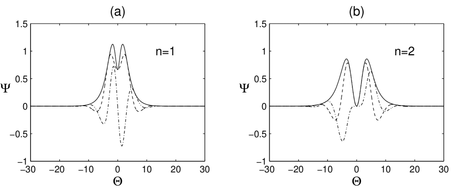
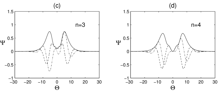
Figure 1: The first four embedded solitons $\Psi(\Theta)$ in Eq. (2.10). The corresponding $\Lambda_{n}$ values $(1\leq n\leq 4)$ are 0.8619, 0.6959, 0.6316 and 0.5939 respectively. Solid lines: $|\Psi|$; dashed lines: Re($\Psi$); dash-dotted lines: Im($\Psi$).

Embedded solitons in equation (2.3) for $\psi$ can now be obtained from those in Eq. (2.10) through the gauge transformation (2.7) – (2.9). We find that embedded solitons $\psi$ exist on the following infinite number of continuous curves in the $(v,\lambda)$ plane:

$$\lambda=\Lambda_{n}\left(v+\frac{1}{3}\right)^{\frac{3}{2}}-\frac{1}{3}v-\frac{2}{27}.$$ (2.13)

The first four such curves ($1\leq n\leq 4$) as well as the limit curve ($n\to\infty$) are shown in Fig. 2(a). On each one of these curves, a continuous family of embedded solitons $\psi$ exists. Note that the velocities of these families of embedded solitons have a common lower bound, $v\geq-\frac{1}{3}$, but there are no upper bounds. Thus, for any velocity $v>-\frac{1}{3}$, a discrete infinite set of embedded solitons can be found. If $v<-\frac{1}{3}$, these solitons disappear. Frequency $\lambda$ also has a lower bound whose value depends on the individual solution family. But $\lambda\geq 0$ holds for all families. On each solution curve, when $\lambda<\frac{1}{27}$ but above the lower $\lambda$ bound of that family, two embedded solitons with different velocities exist.

The energy of an embedded soliton is an important quantity. Here we define the energy as

$$E(\lambda,v)=\int_{-\infty}^{\infty}|\psi(\theta)|^{2}d\theta.$$ (2.14)

Utilizing the gauge transformation (2.7), we easily find that

$$E(\lambda,v)=\beta_{n}\left(v+\frac{1}{3}\right),$$ (2.15)

where $\beta_{n}=\int_{-\infty}^{\infty}|\Psi(\Theta)|^{2}d\Theta$. The first four $\beta_{n}$ values $(1\leq n\leq 4)$ are 7.5434, 5.2786, 4.6916 and 4.3951 respectively. Formula (2.15) indicates that the energy of an embedded soliton increases linearly with velocity. Eliminating $v$ from Eqs. (2.13) and (2.15), we find that the energy $E$ is related to the frequency $\lambda$ as

$$\lambda=\Lambda_{n}\left(\frac{E}{\beta_{n}}\right)^{\frac{3}{2}}-\frac{E}{3\beta_{n}}+\frac{1}{27}.$$ (2.16)

The first four $(\lambda,E)$ curves are displayed in Fig. 2(b). Note that on each energy curve, when $\lambda<\frac{1}{27}$, two embedded solitons with different energies exist.

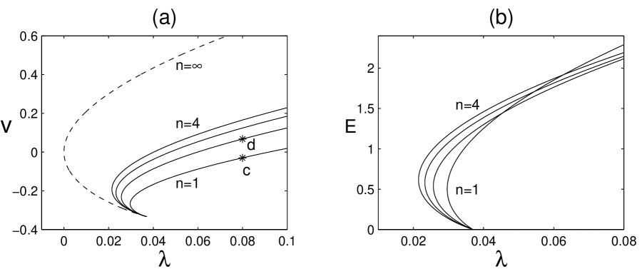
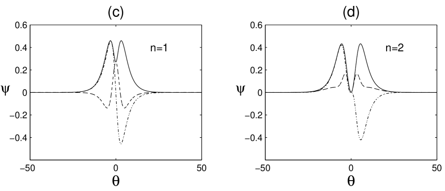
Figure 2: (a, b) Families of curves in the parameter planes $(\lambda,v)$ and $(\lambda,E)$ where embedded solitons $\psi$ exist in the TNLS equation (2.3). (c, d) Profiles of embedded solitons at velocity and frequency values marked as ‘c’ and ‘d’ in figure (a) respectively. Solid lines: $|\psi|$; dashed lines: Re($\psi$); dash-dotted lines: Im($\psi$).

The profiles of embedded solitons $\psi(\theta)$ in the above solution families can be readily deduced from the embedded solitons $\Psi(\Theta)$ through the gauge transformation (2.7) – (2.9). To illustrate typical embedded solitons $\psi$ of Eq. (2.3), we select two points in Fig. 2(a) marked as ‘c’ and ‘d’, which belong to the first and second solution families respectively. The coordinates of these two points are approximately $(\lambda,v)=(0.08,-0.03)$ and $(0.08,0.0674)$. Embedded solitons at these two points are shown in Fig. 2(c, d). We see that their amplitude profiles ($|\psi|$) are similar to those in Fig. 1(a, b) save for horizontal and vertical rescalings, while their phase distributions are different. The reason is apparently due to the gauge transformation (2.7) – (2.9).

It is interesting to note that all solution families in Fig. 2(a) emanate from the single point $(\lambda_{c},v_{c})=(\frac{1}{27},-\frac{1}{3})$ which, according to (2.7), corresponds to the linear limit ($|\psi|\to 0$) of those soliton solutions. The significance of this critical point may also be seen by considering infinitesimal normal-mode disturbances $e^{i\kappa\theta}$ and examining the linear spectrum of Eq. (2.3):

$$F(\kappa;\lambda,v)\equiv\kappa^{3}+\kappa^{2}-v\kappa+\lambda=0.$$ (2.17)

Clearly, (2.17) has either three real or one real and a pair of complex conjugate roots. Based on prior experience [25, 26, 27], one then would expect small-amplitude solitary waves, in the form of wave packets, to bifurcate from infinitesimal sinusoidal disturbances having (real) wavenumber $\kappa_{c}$ that corresponds to a triple root of the linear spectrum:

$$F(\kappa_{c};\lambda_{c},v_{c})=0,\hskip 8.5359ptF^{\prime}(\kappa_{c};\lambda_{c},v_{c})=0,\hskip 8.5359ptF^{\prime\prime}(\kappa_{c};\lambda_{c},v_{c})=0.$$ (2.18)

The critical point $(\lambda_{c},v_{c})$ in Fig. 2(a) is consistent with these conditions, and the value of the critical wavenumber is found to be $\kappa_{c}=-\frac{1}{3}$. The second of conditions (2.18), in particular, implies that the “phase speed” $v$ of linear sinusoidal waves is stationary at critical conditions and hence is equal to the group velocity there. (Note: in this interpretation of phase speed and group speed, the frequency shift $\lambda$ introduced in Eq. (2.1) is treated as a free parameter.) Accordingly, small-amplitude solitary wavepackets close to the bifurcation point may also be interpreted as envelope solitons with stationary crests [25, 26, 27]. Fig. 3 displays one such embedded-soliton wavepacket which belongs to the fourth family. One difference between wave packets here and those in [25, 26, 27], however, is that the present wave packets are embedded solitons, while those in [25, 26, 27] are not.

Figure 3: Embedded solitons near the bifurcation point ($\lambda_{c},v_{c})=(1/27,-1/3)$. (a) enlargement of $(\lambda,v)$ curves for embedded solitons near this point; (b) an embedded soliton of the fourth family at the point marked ‘b’ in figure (a). Solid line: Re($\psi$); dashed line: Im($\psi$).

We remark here that the infinite families of embedded solitons displayed in Fig. 2 are not the only possible embedded solitons $\psi$ of Eq. (2.3). Equivalently, the infinite discrete set of embedded solitons, the first four of which are displayed in Fig. 1, are not the only possible embedded solitons $\Psi$ of Eq. (2.10). The solitons we have studied above have two major humps in their amplitude profiles. Calvo and Akylas [9] have shown that embedded solitons with three or more major humps exist as well. In this paper, we shall not discuss those more complicated solitons.

3 Linear and nonlinear stability of embedded solitons

We now turn to the stability properties of the families of embedded solitons found in the last section. This problem has been considered in [8, 10] for certain isolated embedded solitons. It was suggested that they are linearly weakly unstable, but nonlinearity has a stabilizing effect, permitting those solitons to propagate for long time without breakup [10]. On the other hand, we have seen in the above section that when $\lambda<\frac{1}{27}$, there exist two branches of embedded solitons in the same family having different energy [see Fig. 2(b)]. In such a case, it is typically expected from saddle-node bifurcations in dynamical systems that one branch of solutions is stable, while the other branch is unstable [28]. If this holds also for the TNLS equation, then one would expect different stability properties for the two branches of embedded solitons in the same solution family. Previous work also shows that while single-hump (fundamental) solitons are often linearly stable, multi-hump solitons (whether embedded or not) are often linearly unstable [5, 23]. This fact suggests that embedded solitons in the TNLS equation, or at least higher families ($n\geq 2$) of such solitons, might be linearly unstable. If embedded solitons are linearly stable, nonlinearly they could be semi-stable, i.e., whether they persist or break up depends on the type of initial perturbations imposed. This semi-stability property has been established rigorously for isolated embedded solitons in Hamiltonian systems [5, 14, 18, 22, 23]. For the TNLS equation, embedded solitons exist as continuous families. Thus, when they are perturbed, they may be able to shed some energy via radiation and tend to nearby embedded solitons in the same solution family. If this happens, these embedded solitons could be nonlinearly stable.

In this section, we will establish, however, that the stability properties of embedded solitons in the TNLS equation (1.2) do not follow the above common scenarios. In particular, we will show that for the TNLS equation, (i) all embedded solitons in the same family have identical linear and nonlinear stability properties; (ii) all families of embedded solitons are linearly stable; (iii) embedded solitons are nonlinearly semi-stable at least for the first and second families. The first result can be easily seen from the fact that all embedded solitons in the TNLS equation are related to each other by the gauge transformation (2.7) – (2.9), thus they must be either all stable or all unstable. This contrasts other physical systems where different branches in the same solution family have different stability properties [28]. The second and third results will be established in the following two subsections.

3.1 Linear stability of embedded solitons

To study the linear stability of embedded solitons (2.1) in the TNLS equation (1.2), we write

$$\phi(x,t)=e^{i\lambda t}\left\{\psi(\theta)+\tilde{\phi}(\theta,t)\right\},$$ (3.1)

where $\tilde{\phi}$ is an infinitesimal perturbation, and $\theta$ is defined in (2.2). The linearized equation for $\tilde{\phi}$ is

$$i\tilde{\phi}_{t}-\lambda\tilde{\phi}-iv\tilde{\phi}_{\theta}+\tilde{\phi}_{xx}+2|\psi|^{2}\tilde{\phi}+\psi^{2}\tilde{\phi}^{*}-i\tilde{\phi}_{\theta\theta\theta}=0.$$ (3.2)

To determine the linear stability of these solitons, we numerically simulate the above linearized equation to see if its solution $\tilde{\phi}$ has exponentially growing modes or not. Since a whole family of embedded solitons has the same stability behavior, we only need to pick one embedded soliton from each family and test its linear stability. The numerical scheme we use is the pseudo-spectral method (FFT) along the $x$-direction, and the fourth-order Runge–Kutta method in $t$. For simplicity, we choose a Gaussian initial condition

$$\tilde{\phi}(\theta,0)=(1+i)e^{-\frac{1}{2}\theta^{2}}.$$ (3.3)

Other initial conditions have been used as well, and the results are qualitatively the same.

In the first family of embedded solitons ($n=1$, see Fig. 2), we choose the soliton as displayed in Fig. 2(c), whose frequency and velocity values are $(\lambda,v)=(0.08,-0.03)$. For this soliton, the evolution of the disturbance $\tilde{\phi}$ is shown in Fig. 4. Note that Fig. 4(a) is qualitatively the same as Fig. 3 in Ref. [10]. We see that the disturbance grows. In [10], this was interpreted as weak exponential growth. However, Fig. 4(b) reveals that the disturbance grows only linearly. This linear growth just corresponds to an adjustment of this soliton’s frequency and velocity values, and it is not a sign of linear instability. Thus, this embedded soliton, or equivalently the first family of embedded solitons, is linearly stable.

It is not difficult to determine the origin of this linear growth in the disturbance $\tilde{\phi}$. In fact, the linearly growing mode

$$\tilde{\phi}(\theta,t)=\alpha_{1}\left[i\psi t+\frac{\partial\psi}{\partial\lambda}\right]_{(\lambda_{0},v_{0})}+\alpha_{2}\left[\frac{\partial\psi}{\partial\theta}t-\frac{\partial\psi}{\partial v}\right]_{(\lambda_{0},v_{0})}$$ (3.4)

is a particular solution of the linearized equation (3.2). Here $\alpha_{1}$ and $\alpha_{2}$ are arbitrary real constants, $\psi=\psi(\theta,\lambda,v)$ is the solution of Eq. (2.3) for general $(\lambda,v)$ values (which is generally nonlocal), and $(\lambda_{0},v_{0})$ are the embedded soliton’s frequency and velocity parameters. A general initial perturbation $\tilde{\phi}(\theta,0)$ excites this mode, thus the disturbance grows linearly in time. But this mode does not imply exponential instability. An analogous situation is the NLS soliton under perturbations (see [29, 30]).

Are other families of embedded solitons with $n\geq 2$ linearly stable? To answer this question, we have repeated the above numerical simulation for embedded solitons in the higher families, and found that they are all linearly stable. To illustrate, we consider the second family, and pick the embedded soliton as shown in Fig. 2(d), where the frequency and velocity parameters are $(\lambda,v)=(0.08,0.0674)$. With the same Gaussian initial condition (3.3), evolution of the disturbance $\tilde{\phi}$ is displayed in Fig. 5. We see that, just like the first family, the disturbance grows linearly, which implies that the second solution family is linearly stable as well.

Figure 4: Evolution of infinitesimal perturbations to the embedded soliton of the first family, shown in Fig. 2(c).

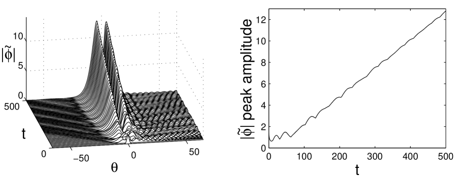
Figure 5: Evolution of infinitesimal perturbations to the embedded soliton of the second family, shown in Fig. 2(d).

3.2 Nonlinear semi-stability of embedded solitons

As we have shown above, embedded solitons in the TNLS equation (1.2) exist as continuous families, and they are all linearly stable. Are they also nonlinearly stable to small perturbations? If embedded solitons are isolated in a Hamiltonian system, these solitons are generally semi-stable [5, 14, 18, 22, 23]. The reason can be understood heuristically as follows [5]. When an isolated embedded soliton is perturbed, it will tend to an adjacent state which is not locally confined, but features tails of non-zero amplitude. However, it would require infinite energy to create a non-vanishing tail. Because the energy is conserved in a Hamiltonian system, and the energy $E_{0}$ of the unperturbed embedded soliton is finite, there are two possibilities: first, if the initial perturbed state has a total energy $E<E_{0}$, the energy lost in an attempt to generate the infinite tail will drive the soliton farther away from the initial state. As a result, the perturbed embedded soliton can be expected to eventually decay into radiation. On the other hand, if the initial perturbed state has energy $E>E_{0}$, we may expect the energy lost in generating the tail to drag the pulse back toward the unperturbed embedded soliton. Thus, we can anticipate that the embedded soliton is subject to a non-exponential one-sided instability which is the so-called semi-stability.

However, embedded solitons in the TNLS equation (1.2) are continuous rather than isolated. These solitons have a free parameter which is their velocity. In addition, their energy depends linearly on their velocity [see Eq. (2.15)], thus their energy can acquire an arbitrary value. Because of this, the above argument for semi-stability no longer holds for embedded solitons in the TNLS equation. When an embedded soliton in the TNLS equation is perturbed, in principle, it could simply emit some radiation and adjust its shape to a nearby embedded soliton in the same solution family, as an NLS soliton does under perturbations. This prospect originally led us to speculate that embedded solitons in the TNLS equation may actually be nonlinearly stable. Unfortunately, this speculation turns out to be incorrect. Our numerical simulations show that these solitons are still semi-stable, just like isolated embedded solitons in other physical systems [5, 13, 14, 18]. In other words, the freedom of arbitrary velocities of embedded solitons in the TNLS equation is not sufficient to stabilize these solitons.

To explore the nonlinear stability of embedded solitons in the TNLS equation, we numerically simulate this equation starting with an embedded soliton under perturbations. Since a whole family of embedded solitons have the same stability properties, it is sufficient to pick one soliton from each family and test its stability. In numerical simulations, we adopt the coordinates which move at the speed $v$ of the embedded soliton. Then the TNLS equation (1.2) becomes

$$i\phi_{t}-iv\phi_{\theta}+\phi_{\theta\theta}+|\phi|^{2}\phi=i\phi_{\theta\theta\theta},$$ (3.5)

where $\theta$ has been defined in Eq. (2.2). In these coordinates, an embedded soliton is given by (2.1). Consistent with the initial perturbations which we have used in other wave systems which admit embedded solitons [5, 14, 18, 23], we use the initial condition

$$\phi(\theta,0)=(1+\alpha)\psi(\theta),$$ (3.6)

where $\alpha$ is a small real constant. That is, our initial perturbed state is the original soliton amplified by a factor $1+\alpha$. In this case, the energy of the initial state is $(1+\alpha)^{2}$ multiplied by the energy of the unperturbed soliton [see Eq. (2.14)]. When $\alpha>0$, the perturbed state has higher energy than the unperturbed soliton, while when $\alpha<0$, the perturbed state has lower energy than the unperturbed soliton. In previous studies on isolated embedded solitons, we have termed the former perturbations as “energy increasing”, and the latter perturbations as “energy decreasing” [5, 14, 18]. However, in the present case, we will refrain from using such terms. The reason is that embedded solitons here are continuous, so is their energy. Thus it may be ambiguous or even confusing to say “energy-increasing or -decreasing perturbations”. Other initial perturbations different from (3.6) can also be taken, but they are not expected to change the qualitative conclusions.

Because of the gauge transformation (2.7) – (2.9), it makes no difference which embedded soliton $\psi(\theta)$ in a solution family we use in our simulations. In other words, for a fixed value of $\alpha$, whether the perturbed state (3.6) eventually breaks up or persists is independent of the choice of the embedded soliton in a solution family.

We first consider the first family of embedded solitons. Extensive numerical simulations have shown that this family of embedded solitons persist when $0\leq\alpha\>^{<}_{\sim}\>0.081$, while they break up otherwise. The simulation results for three values of $\alpha$, $-0.02$, 0.08 and 0.09, are plotted in Fig. 6, where the particular soliton used is as displayed in Fig. 2(c) with $(\lambda,v)=(0.08,-0.03)$. We see that for $\alpha=-0.02$, the embedded soliton sheds continuous-wave radiation whose amplitude steadily increases over time. As a result, the soliton breaks up. This behavior is typical of isolated embedded solitons under energy-decreasing perturbations [5, 14, 18]. For $\alpha=0.08$, the soliton also sheds continuous-wave radiation, but the radiation tail decreases over time. Meanwhile, the central pulse adjusts itself and approaches a nearby embedded soliton with a higher velocity. As a result, the soliton persists under this perturbation. This behavior is somewhat similar to isolated embedded solitons under energy-increasing perturbations [5, 14, 18]. However, the new feature here is that the final embedded soliton is different from the unperturbed soliton, although the final soliton clearly still belongs to the first family. What happens here is that part of the increased energy in the initial perturbed state is absorbed by the original soliton and changes it to a nearby soliton with higher energy (velocity), while the rest of the increased energy radiates away. For $\alpha=0.09$, however, the situation is different. Initially, the perturbed state appears to adjust itself toward a nearby soliton with higher energy (velocity). But later on, the tail radiation starts to increase, which eventually breaks up the soliton. We have checked all these simulations with higher accuracy and over longer periods of time, and the results remain the same. It is noted that our numerical results above are consistent with previous numerical simulations by Calvo and Akylas [10].

The above numerical results indicate that the first family of embedded solitons are semi-stable: whether the soliton persists or breaks up depends on the initial perturbation. Compared to the dynamics of isolated embedded solitons, a new feature we find here is that embedded solitons are unstable not only for $\alpha<0$, but also for $\alpha$ above a certain threshold value (which is 0.081 here). At the present time, the reason for this new behavior is still not clear. It could be because when $\alpha>0.081$, the perturbation becomes too strong for this double-humped embedded soliton. As we know, any soliton can be broken up with a strong enough perturbation. But the fact that the perturbed state initially does adjust itself toward a nearby soliton makes us suspect that the reason for its eventual breakup may be elsewhere [see Fig. 6(c)]. A full explanation for this new behavior may be obtained from a detailed internal-perturbation calculation as has been done for isolated embedded solitons in several other physical systems [14, 18]. But this remains to be seen.

Are higher families of embedded solitons also semi-stable? To explore this question, we have repeated the above simulations for an embedded soliton in the second family. The initial perturbation remains the same as in (3.6). In this case, we have found that the second family of embedded solitons is stable only when $0\leq\alpha\>^{<}_{\sim}\>0.018$, and breaks up otherwise. Three simulation results with $\alpha=-0.01,0.015$ and 0.02 are plotted in Fig. 7, where the particular embedded soliton used is the one shown in Fig. 2(d) with $(\lambda,v)=(0.08,0.0674)$. These results are qualitatively the same as for the first family, but the window of $\alpha$ for soliton stability is much narrower. In other words, embedded solitons of the second family are more prone to breakup under perturbations. For the third family of embedded solitons, our numerical simulations did not find a window of $\alpha$ for soliton persistence. This may be because that window is too small and we did not detect it. It is also possible that such a window actually disappears for the third (and higher) families of embedded solitons. This issue is not pursued further in this paper.

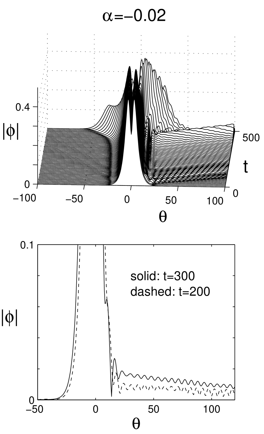
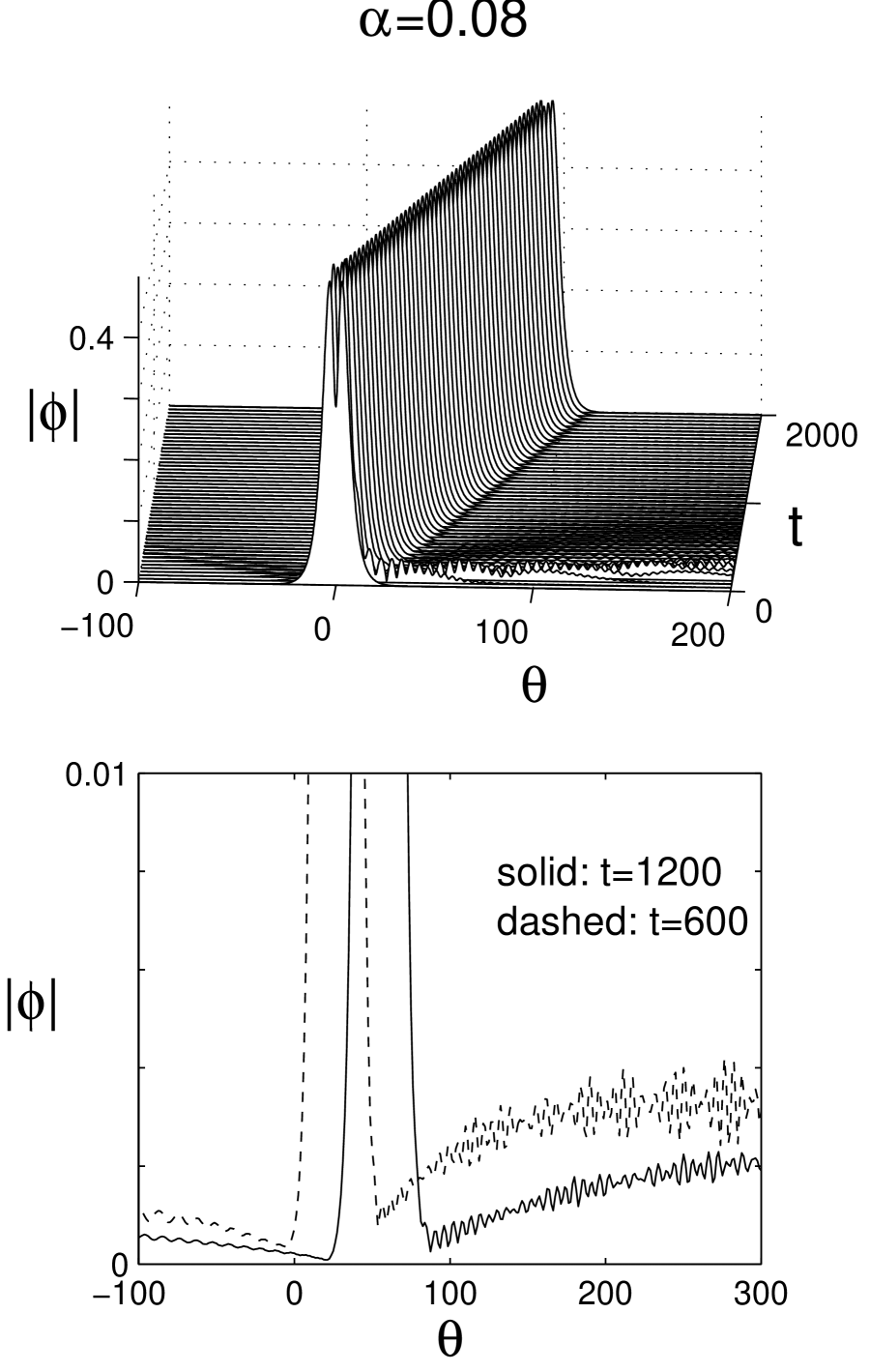
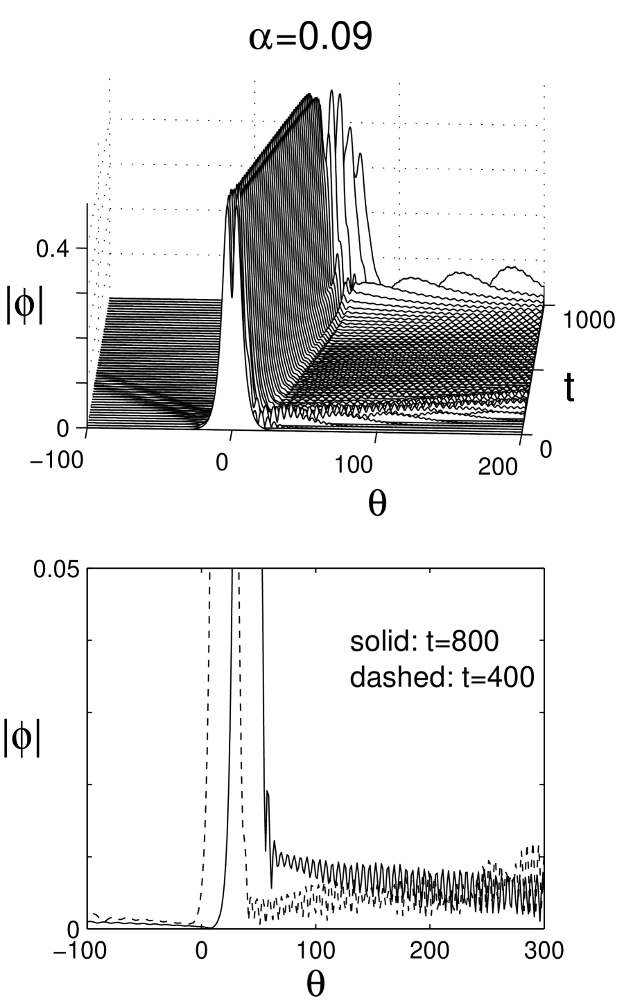
Figure 6: Evolution of the embedded soliton of the first family, shown in Fig. 2(c), under perturbations (3.6) for various values of $\alpha$. First column: $\alpha=-0.02$; second column: $\alpha=0.08$; third column: $\alpha=0.09$.

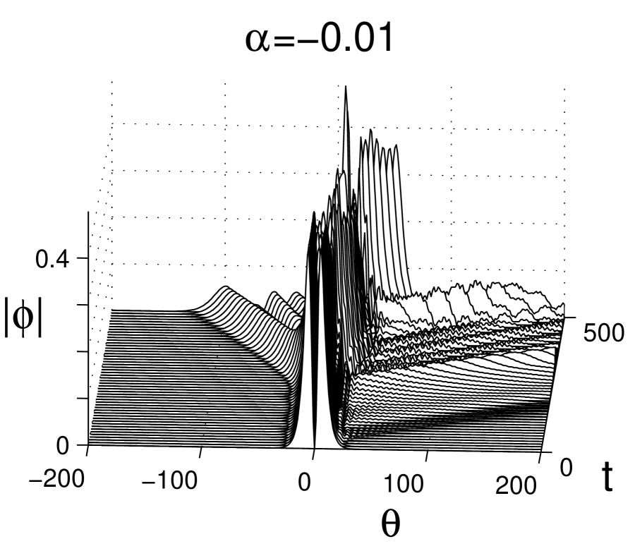
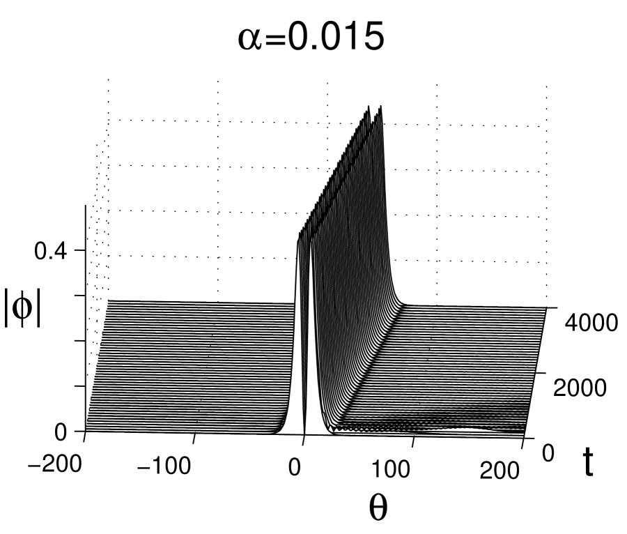
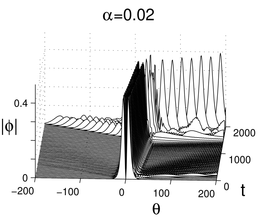
Figure 7: Evolution of the embedded soliton of the second family, shown in Fig. 2(d), under perturbations (3.6) for various values of $\alpha$.

4 Discussion

In this article, we have studied embedded solitons and their stability in the third-order NLS equation (1.2). We have discovered an infinite number of continuous families of embedded solitons parameterized by their velocities, or equivalently by their energies. We have further shown that these families of embedded solitons are all linearly stable. But nonlinearly they are still semi-stable, just like isolated embedded solitons in other physical systems [5, 14, 18].

In the theory of embedded solitons, the following question still remains open: are nonlinearly stable embedded solitons in Hamiltonian systems possible or not? This question is quite important for physical applications. Previous work has made it clear that a necessary condition for such embedded solitons to be possible is that they exist as continuous families, not as isolated solutions [5, 14, 18]. However, our results in this paper indicate that this condition is apparently not sufficient. Whether other physical systems support nonlinearly stable embedded solitons or not needs further investigation.

References

- [1] G.P. Agrawal, Nonlinear Fiber Optics. Academic Press, San Diego, 1989.
- [2] Hasegawa, A. and Kodama, Y., “Solitons in Optical Communications.” Clarendon Press, Oxford, 1995.
- [3] P.K.A. Wai, H.H. Chen and Y.C. Lee, “Radiation by solitons at the zero group dispersion wavelength of single-mode optical fibers.” Phys. Rev. A 41, 426 (1990).
- [4] T.R. Akylas and T.J. Kung, “On nonlinear wave envelopes of permanent form near a caustic.” J. Fluid Mech. 214, 489 (1990).
- [5] J. Yang, B.A. Malomed, and D.J. Kaup, “Embedded solitons in second-harmonic-generating systems”, Phys. Rev. Lett. 83, 1958 (1999).
- [6] P.S. Jang and D.J. Benney, Dynamics Technology, Inc. Tech. Report No. DT-8167-1 (1981), unpublished.
- [7] H.A. Haus, J.D. Moores and L.E. Nelson, “Effect of third-order dispersion on passive mode locking.” Opt. Lett. 18, 51 (1993).
- [8] M. Klauder, E.W. Laedke, K.H. Spatschek, and S.K. Turitsyn, “Pulse propagation in optical fibers near the zero dispersion point.” Phys. Rev. E 47, R3844 (1993).
- [9] D.C. Calvo and T.R. Akylas, “On the formation of bound states by interacting nonlocal solitary waves.” Physica D 101, 270 (1997).
- [10] D.C. Calvo and T.R. Akylas, “Stability of bound states near the zero-dispersion wavelength in optical fibers.” Phys. Rev. E 56, 4757 (1997).
- [11] S. Kichenassamy and P.J. Olver, “Existence and nonexistence of solitary wave solutions to higher-order model evolution equations”, SIAM J. Math. Anal. 23, 1141 (1992).
- [12] A.R. Champneys and M.D. Groves, “A global investigation of solitary wave solutions to a two-parameter model for water waves”, J. Fluid Mech. 342, 199 (1997).
- [13] J. Yang, “Dynamics of embedded solitons in the extended KdV equations.” Stud. Appl. Math. 106, 337 (2001).
- [14] Y. Tan, J. Yang and D.E. Pelinovsky, “Semi-stability of embedded solitons in the general fifth-order KdV equation.” Wave Motion 36, 241 (2002).
- [15] A.V. Buryak, “Stationary soliton bound states existing in resonance with linear waves”, Phys. Rev. E 52, 1156 (1995).
- [16] J. Fujioka and A. Espinosa, “Soliton-like solution of an extended NLS equation existing in resonance with linear dispersive waves”, J. Phys. Soc. Japan 66, 2601 (1997).
- [17] R. Grimshaw and P. Cook, “Solitary waves with oscillatory tails”, in Proceedings of the Second International Conference on Hydrodynamics, editors: A.T. Chwang, J.H.W. Lee, and D.Y.C. Leung, Hong Kong, 1996, 327.
- [18] D.E. Pelinovsky, and J. Yang, “A normal form for nonlinear resonance of embedded solitons.” Proc. Roy. Soc. Lond. A. 458, 1469-1497 (2002).
- [19] A.R. Champneys, and B.A. Malomed, and M.J. Friedman, “Thirring solitons in the presence of dispersion”, Phys. Rev. Lett. 80, 4169 (1998).
- [20] A.R, Champneys and B.A. Malomed, “Moving embedded solitons”, J. Phys. A 32, L547 (1999).
- [21] A.R. Champneys and B.A. Malomed, “Embedded solitons in a three-wave system”, Phys. Rev. E 61, 886 (1999).
- [22] A.R. Champneys, B.A. Malomed, J. Yang, and D.J. Kaup, “Embedded solitons: solitary waves in resonance with the linear spectrum”. Physica D 152, 340 (2001).
- [23] J. Yang, B.A. Malomed, D.J. Kaup, and A.R. Champneys, “Embedded solitons: a new type of solitary waves”. Mathematics and Computers in Simulation, 56, 585 (2001).
- [24] Ueda, T. and Kath, W.L. “Dynamics of coupled solitons in nonlinear optical fibers.” Phys. Rev. A 42, 563 (1990).
- [25] T.R. Akylas, “Envelope solitons with stationary crests.” Phys. Fluids A 5, 789 (1993).
- [26] R. Grimshaw, B. Malomed and E. Benilov, “Solitary waves with damped oscillatory tails: an analysis of the fifth-order Korteweg–de Vries equation.” Physica D 77, 473 (1994).
- [27] T.S. Yang and T.R. Akylas, “On asymmetric gravity–capillary solitary waves.” J. Fluid Mech. 330, 215 (1997).
- [28] D.E. Pelinovsky, ”Instabilities of dispersion-managed solitons in the normal dispersion regime.” Phys. Rev. E 62, 4283 (2000).
- [29] D.J. Kaup, “Perturbation theory for solitons in optical fibers.” Phys. Rev. A 42, 5689 (1990).
- [30] J. Yang, ”Vector solitons and their internal oscillations in birefringent nonlinear optical fibers.” Stud. Appl. Math. 98, 61-97 (1997).