Quiescent String Dominance Parameter F and Classification of One-Dimensional Cellular Automata

Abstract

The mechanism which discriminates the pattern classes at the same $\lambda$, is found. It is closely related to the structure of the rule table and expressed by the numbers of the rules which break the strings of the quiescent states. It is shown that for the N-neighbor and K-state cellular automata, the class I, class II, class III and class IV patterns coexist at least in the range, $\frac{1}{K}\leq\lambda\leq 1-\frac{1}{K}$. The mechanism is studied quantitatively by introducing a new parameter $F$, which we call quiescent string dominance parameter. It is taken to be orthogonal to $\lambda$. Using the parameter F and $\lambda$, the rule tables of one dimensional 5-neighbor and 4-state cellular automata are classified. The distribution of the four pattern classes in ($\lambda$,F) plane shows that the rule tables of class III pattern class are distributed in larger $F$ region, while those of class II and class I pattern classes are found in the smaller $F$ region and the class IV behaviors are observed in the overlap region between them. These distributions are almost independent of $\lambda$ at least in the range $0.25\leq\lambda\leq 0.75$, namely the overlapping region in $F$, where the class III and class II patterns coexist, has quite gentle $\lambda$ dependence in this $\lambda$ region. Therefore the relation between the pattern classes and the $\lambda$ parameter is not observed.

I Introduction

Cellular automata (CA) has been one of the most studied fields in the research of complex systems. Various patterns has been generated by choosing the rule tables. Wolframwolfram has classified these patterns into four rough categories: class I (homogeneous), class II (periodic), class III (chaos) and class IV (edge of chaos). The class IV patterns have been the most interesting target for the study of CA, because it provides us with an example of the self-organization in a simple system and it is argued that the possibility of computation is realized by the complexity at the edge of chaoswolframs ; langton .
Much more detailed classifications of CA, have been carried out mainly for the elementary cellular automata (3-neighbor and 2-state CA)hanson ; wuensche , in which the patterns are studied quite accurately for each rule table. And the classification of the rule tables are studied by introducing some parametersbinder ; wuensche ; oliveira . However, in this case, there are some confusions in the classification of the class IV CA. The result on the so to speak $\rho=1/2$ task from Packardpackard have been different from that of Mitchell, Crutchfield and Hrabermitchell . In this case, the number of the independent rule tables are so small to treat them statistically and the symmetry of the interchange of the states ”0” and ”1” make the classifications of the the pattern classes more delicate than those of other CA with $K\geq 3$. Therefore, it may be worth to start with other models, in order to find the general properties of the CA.
However the number of rule tables in N-neighbor and K-state cellular automata CA(N,K) grows like $K^{K^{N}}$. Therefore except for a few smallest combinations of the $N$ and $K$, the numbers of the rule tables become so large that studies of the CA dynamics for all rule tables are impossible even with the fastest supercomputers. Therefore it is important to find a set of parameters by which the pattern classes could be classified , even if it is a qualitative one.
Langton has introduced $\lambda$ parameter and argued that as $\lambda$ increases the pattern class changes from class I to class II and then to class III. And class IV behavior is observed between class II and class III pattern classeslangton0 ; langton ; langton2 . The $\lambda$ parameter represents rough behavior of CA in the rule table space, but finally does not sufficiently classify the quantitative behavior of CA. It is well known that different pattern classes coexist at the same $\lambda$. Which of these pattern classes is chosen, depends on the random numbers in generating the rule tables. The reason or mechanism for this is not yet known; we have no way to control the pattern classes at fixed $\lambda$. And the transitions from a periodic to chaotic pattern classes are observed in a rather wide range of $\lambda$. In Ref.langton2 , a schematic phase-diagram was sketched. However a vertical axis was not specified. Therefore, it has been thought that new parameters are necessary to arrive at more quantitative understandings of the rule table space of the CA .
In this article, we will clarify the mechanism which discriminate the class I, class II, class III and class IV pattern classes at fixed $\lambda$. It is closely related to the structure of the rule tables; numbers of rules which breaks strings of quiescent states. It is studied quantitatively by introducing a new parameter $F$, which we will call quiescent string dominance parameter. It is taken to be orthogonal to $\lambda$. In the region $1/K\leq\lambda\leq 1-1/K$, the maximum of $F$ corresponds to class III rule tables while minimum of $F$, to class II or class I rule tables. Therefore the transition of the pattern classes takes place somewhere between these two limits without fail. By the determination of the region of $F$, where the change of the pattern classes takes place, we could obtain the phase diagram in ($\lambda$,F) plane, and classify the rule table space.
The determination of the phase diagram is carried out for CA(5,4). It is found that the rule tables are not separated by a sharp boundaries but they are represented by probability densities. Therefore we define the equilibrium points of two phases where the two probability densities of the pattern classes become equal, and define the transition region where the probability densities of the both pattern classes are not too much different from each other. By using the equilibrium points and the transition region, we draw a phase diagram in ($\lambda$,F) plane.
It is found that $\lambda$ dependences of the equilibrium points and transition region are very gentle, and they continued to be found at least over the range $0.125\leq\lambda\leq 0.75$. It means that all the four pattern classes do coexist over the wide range in $\lambda$. Our results for the distributions of these pattern classes in ($\lambda,F$) plane do not support the well known relation between the pattern classes and the $\lambda$ parameter proposed in the Ref.langton . It will be shown that the results there, are due to the methods to generate the rule tables with probability $\lambda$.
In section II, we briefly summarize our notations and present a key discovery, which leads us to the understanding of the relation between the structure of the rule table and pattern classes. It strongly suggested that the rules which break strings of the quiescent states play an important role for the pattern classes.
In section III, the rule tables are classified according to the destruction and construction of strings of the quiescent states and we find the method to change the chaotic pattern class into periodic one and vice versa while keeping $\lambda$ fixed. We will show that by using the method, the change of the pattern classes takes place without fail, in the region $1/K\leq\lambda\leq 1-1/K$.
In section IV, the result obtained in section III is studied quantitatively by introducing a new quiescent string dominance parameter $F$. It is determined by using the distribution of class IV rule tables, which we call optimal $F$ parameter.
In section V, using $F$ and $\lambda$, we classify the rule tables of CA(5,4) in ($\lambda$,F) plane. It will be shown that all the four pattern classes do coexist in wide range in $\lambda$, contrary to the result of Ref. langton by Langton. The reason why he obtained his result will be discussed.
In section VI, the rule tables of CA(5,4) are classified in the ($\lambda$,F) plane, which provides us with the phase diagram.
Section VII is devoted to discussions and conclusions, where a possibility of the transmission of the initial state information and the classification of the rule tables by the another intuitive $F$ parameter, will be discussed.

II SUMMARY OF CELLULAR AUTOMATA AND A KEY DISCOVERY

II.1 Summary of cellular automata

In order to make our arguments concrete, we focus mainly on the one-dimensional 5-neighbor and 4-state CA (CA(5,4)) in the following, because this is a model in which Langton had argued the classification of CA by the $\lambda$ parameter. However the qualitative conclusions in this article, hold true for general CA(N,K). These points will be discussed in the subsections III B.
We will briefly summarize our notation of CAwolfram ; langton . In our study, the site consists of 150 cells having the periodic boundary condition. The states are denoted as $s(t,i)$. The $t$ represents the time step which takes an integer value, and the $i$ represents the position of cells which range from $0$ to $149$. The $s(t,i)$ takes values $0,1,2,$ and $3$, and the state $0$ is taken to be the quiescent state. The set of the states $s(t,i)$ at a time $t$ is called the configuration.
The configuration at time $t+1$ is determined by that of time $t$ by using following local relation,

$$s(t+1,i)=T(s(t,i-2),s(t,i-1),s(t,i),s(t,i+1),s(t,i+2)).$$ (1)

The set of the mappings

$$T(\mu,\nu,\kappa,\rho,\sigma)=\eta,(\mu,\nu,etc.=0,1,2,3)$$ (2)

is called the rule table. The rule table consists of $4^{5}$ mappings, which is selected from a total of $4^{1024}$ mappings.
The $\lambda$ parameter is defined aslangton0 ; langton

$$\lambda=\frac{N_{h}}{1024},$$ (3)

where $N_{h}$ is the number in which $\eta$ in Eq. (2) is not equal to $0$. In other words the $\lambda$ is the probability that the rules do not select the quiescent state in next time step. Until section III, we set the rule tables randomly with the probability $\lambda$. Our method is to choose $1024-N_{h}$ rules randomly, and set $\eta=0$ in the right hand side of Eq. (2), and for the rest of the $N_{h}$ rules, the $\eta$ picks up the number 1,2 and 3 randomly. The initial configurations are also set randomly.
The time sequence of the configurations is called a pattern. The patterns are classified roughly into four classes established by Wolframwolfram . It is widely accepted that pattern classes are classified by the $\lambda$langton ; as the $\lambda$ increases the most frequently generated patterns change from homogeneous (class I) to periodic (class II) and then to chaotic (class III), and at the region between class II and class III, the edge of chaos (class IV) is located.

II.2 Correlation between pattern classes and rules which break strings of quiescent states

In order to find the reason why the different pattern classes are generated at the same $\lambda$, we have started to collect rule tables of different pattern classes, and tried to find the differences between them. We fix at $N_{h}=450$ ($\lambda=0.44$), because we find empirically that around this point the chaotic, edge of chaos, and periodic patterns are generated with similar ratio. By changing the random number, we have gathered a few tens of the rule tables and classified them into chaotic, edge of chaos, and periodic ones.
In this article, a pattern is considered the edge of chaos (class IV) when its transient lengthlangton is longer than $3000$ time steps.
First, we study whether or not the pattern classes are sensitive to the initial configurations. We fix the rule tables and change the initial configurations randomly. For most of the rule tables, the details of the patterns depend on the initial configurations, but the pattern classes are not changedwolfram . The exceptions will be discussed in the subsection VII A, in connection with the transmission of the initial state information. Thus the differences of the pattern classes are due to the differences in the rule tables, and the target of our inquiry has to do with the differences between them.
For a little while, we do not impose a quiescent condition (QC), $T(0,0,0,0,0)=0$, because without this condition, the structure of the rule table becomes more transparent. This point will further be discussed in section IV.
After some trial and error, we have found a strong correlation between the pattern classes and the QC. The probability of the rule table, which satisfies the QC is much larger in class II patterns than that in the class III patterns. This correlation suggest that the rule $T(0,0,0,0,0)=h,\hskip 5.69046pth\neq 0$, which breaks the string of the quiescent states with length 5, pushes the pattern toward chaos. We anticipate that the similar situation will hold for the length 4 strings of quiescent states.
We go back to the usual definitions of CA; in the following we discuss CA under QC, $T(0,0,0,0,0)=0$. We study the correlation between the number of the rules which breaks the length four strings of the quiescent states. These rules are given by,

$$\begin{array}[]{ll}T(0,0,0,0,i)=h,\\ T(i,0,0,0,0)=h,(i,h=1,2,3).\end{array}$$ (4)

They will also push the pattern toward chaos. Similar properties of the rule tables had been noticed by Wolfram and Suzudo with the arguments of the unbounded growthwolfram and expandabilitysuzudo .
We denote the total number of rules of Eq. (4) in a rule table as $N_{4}$. In order to study the correlation between the pattern classes and the number $N_{4}$, we have collected 30 rule tables and grouped them by the number $N_{4}$. We have 4 rule tables with $N_{4}\geq 4$ , 13 rule tables with $N_{4}=3$, 9 rule tables with $N_{4}=2$ and 4 rule tables with $N_{4}\leq 1$. When $N_{4}\geq 4$, all rule tables generate chaotic patterns, while when $N_{4}\leq 1$, only periodic ones are generated. At $N_{4}=3$ and $N_{4}=2$, chaotic, edge of chaos, and periodic patterns coexist. Examples are shown in the Fig. 1. The coexistence of three pattern classes at $N_{4}=3$ is seen in Fig. 1(b), Fig. 1(c) and Fig. 1(d) and that of $N_{4}=2$ is exhibited in Fig. 1(e), Fig. 1(f) and Fig. 1(g).

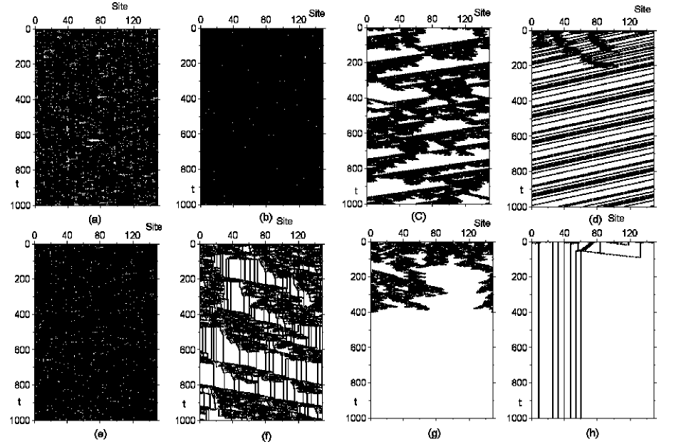
Figure 1: The pattern classes at $N_{h}=450$. The quiescent state is shown by white dot, while other states are indicated by black points. Fig.1(a) corresponds to $N_{4}=4$, Fig. 1(b), Fig. 1(c), and Fig. 1(d), to $N_{4}=3$, Fig. 1(e), Fig. 1(f), and Fig. 1(g), to $N_{4}=2$, and Fig. 1(h) corresponds to $N_{4}=1$, respectively.

As anticipated, the strong correlation between $N_{4}$ and the pattern classes has been observed in this case too. These discoveries have provided us with a key hint leading us to the hypothesis that the rules, which break strings of the quiescent states, will play a major role for the pattern classes.

III Structure of rule table and pattern classes

III.1 Structure of rule table and replacement experiment

In order to test the hypothesis of the previous section, we classify the rules into four groups according to the operation on strings of the quiescent states. In the following, Greek characters in the rules represent groups $0,1,2,3$ while Roman, represent groups $1,2,3$.
Group 1: $T(\mu,\nu,0,\rho,\sigma)=h$.
The rules in this group break strings of the quiescent states.
Group 2: $T(\mu,\nu,0,\rho,\sigma)=0$.
The rules of this group conserve them.
Group 3: $T(\mu,\nu,i,\rho,\sigma)=0$.
The rules of this group develop them.
Group 4: $T(\mu,\nu,i,\rho,\sigma)=l$.
The rules in this group do not affect string of quiescent states in next time step.
Let us denote the number of the group 1 rules in a rule table as $N(g1)$. Similarly for the number of other groups. They satisfy the following sum rules, when $N_{h}$ is fixed.

$$\begin{array}[]{ll}N(g1)+N(g2)=256,\\ N(g3)+N(g4)=768,\\ N(g2)+N(g3)=1024-N_{h},\\ N(g1)+N(g4)=N_{h}.\end{array}$$ (5)

In the methods of generating the rule tables randomly using $N_{h}$ ($\lambda$), these numbers are determined mainly by the probability $\lambda$; namely $N(g1)\simeq 256\lambda$, $N(g2)\simeq 256(1-\lambda)$ $N(g3)\simeq 768(1-\lambda)$ and $N(g4)\simeq 768\lambda$ respectively. Therefore they suffer from fluctuation due to randomness.
The group 1 rules are further classified into five types according to the length of string of quiescent states, which they break. These are shown in Table 1. The rule D5 is always excluded from rule tables by the quiescent condition.

Table 1: The classification of the rules in group 1 into five types, where $h\neq 0$.

type	Total Number	Name	Replacement
$T(0,0,0,0,0)=h$	1	D5	RP5,RC5
$T(0,0,0,0,i)=h$	3	D4	RP4,RC4
$T(i,0,0,0,0)=h$	3
$T(0,0,0,i,\sigma)=h$	12
$T(i,0,0,0,m)=h$	9	D3	RP3,RC3
$T(\mu,j,0,0,0)=h$	12
$T(\mu,j,0,0,m)=h$	36	D2	RP2,RC2
$T(i,0,0,l,\sigma)=h$	36
$T(\mu,j,0,l,\sigma)=h$	144	D1	RP1,RC1

Our hypothesis presented at the end of the section II is expressed more quantitatively as follows; the numbers of the D4, D3, D2, and D1 rules shown in Table 1 will mainly determine the pattern classes.
In order to test this hypothesis, we artificially change the numbers of the rules in Table 1 while keeping the $N_{h}$ ($\lambda$) fixed. For D4 rules, we carry out the replacements defined by the following equations,

$$\begin{array}[]{ll}T(0,0,0,0,i)=h\rightarrow T(0,0,0,0,i)=0,\\ or\hskip 2.84544ptT(i,0,0,0,0)=h\rightarrow T(i,0,0,0,0)=0,\\ T(\mu,\nu,j,\rho,\sigma)=0\rightarrow T(\mu,\nu,j,\rho,\sigma)=l,\\ \end{array}$$ (6)

where except for $h$, the groups $\mu$, $\nu$, $\rho$, $\sigma$, $j$ and $l$ are selected randomly. Similarly the replacements are generalized for D3, D2, and D1 rules , which are denoted as RP4 to RP1 in Table 1. They change the rules of group 1 to that of group 2 together with group 3 to group 4 and are expected to push the rule table toward the periodic direction.
The reverse replacements for D4 are

$$\begin{array}[]{ll}T(0,0,0,0,i)=0\rightarrow T(0,0,0,0,i)=h,\\ or\hskip 2.84544ptT(i,0,0,0,0)=0\rightarrow T(i,0,0,0,0)=h,\\ T(\mu,\nu,j,\rho,\sigma)=l\rightarrow T(\mu,\nu,j,\rho,\sigma)=0,\\ \end{array}$$ (7)

which will push the rule table toward the chaotic direction. In this case, the groups $h$, $\mu$, $\nu$, $j$, $\rho$, and $\sigma$ are selected randomly. Similarly we introduce the replacements for D3, D2, and D1, which will be called RC4 to RC1 in the following.
By the replacement of RP4 to RP1 or RC4 to RC1, we change the numbers of the rules in Table 1 while keeping the $N_{h}$ fixed. We denote these numbers $N_{4}$, $N_{3}$, $N_{2}$, and $N_{1}$ for D4, D3, D2, and D1 rules, respectively. By applying these replacements, we could study the rule tables which are difficult to obtain using only $N_{h}$ ($\lambda$).
Examples of the replacement experiments are shown in Fig. 2.

Figure 2: An example of the replacement experiments at $N_{h}=615$. Fig. 2(a) is obtained randomly with $N_{h}=615$ ($\lambda=0.6)$, by the method explained in subsection II A. Fig. 2(b) to Fig. 2(h) are obtained by the replacements of the rule table of Fig. 2(a), which are summarized in Table 2.

Table 2: The numbers of the group 1 rules and numbers of the replacements for the rule table of Fig. 2(a) to change the patten classes shown in Fig. 2

Figure	$N_{4}$	$N_{3}$	$N_{2}$	$N_{1}$	RP4	RP3	RP2	RP1
Fig. 2(a)	3	22	53	96	0	0	0	0
Fig. 2(b)	0	14	53	96	3	8	0	0
Fig. 2(c)	0	13	53	96	3	9	0	0
Fig. 2(d)	0	12	53	96	3	10	0	0
Fig. 2(e)	1	7	53	96	2	15	0	0
Fig. 2(f)	1	6	53	96	2	16	0	0
Fig. 2(g)	2	1	53	96	1	21	0	0
Fig. 2(h)	2	0	53	96	1	22	0	0

In this replacements, the RP4s are always carried out first, after that RP3s are done. The rule table of Fig. 2(a) is obtained randomly with $N_{h}=615$ ($\lambda=0.6)$. The numbers of the D4, D3, D2 and D1 are shown in line Fig. 2(a) of Table 2. At $N_{h}=615$ most of the randomly obtained rule tables generate chaotic patterns. We start to make RP4 tree times, then number of the D4 becomes $N_{4}=0$. At this stage, the rule table still generate chaotic patterns. Then we proceed to carry out RP3. The chaotic patterns continues from $N_{3}=22$ to $N_{3}=15$, and when $N_{3}$ becomes $14$, the pattern changes to edge of chaos behavior, which is shown in the Fig. 2(b). Fig. 2(c) is obtained by one more RP3 replacements for Fig. 2(b) rule table. It shows a periodic pattern with a rather long transient length. The pattern with one more replacement of RP3 for the Fig. 2(c), is shown in Fig. 2(d), where the transient length becomes shorter. These numbers of D4 rule ($N_{4}$) and D3 rule ($N_{3}$), and numbers of the replacements RP4s and RP3s for the Fig. 2(a) rule table, are summarized in Table 2.
Similarly replacement experiments in which the RP4s are stopped at $N_{4}=1$ and $N_{4}=2$ are shown in Fig. 2(e), Fig. 2(f), and Fig. 2(g), Fig. 2(h), respectively and the numbers of group 1 rules and the replacements are also summarized in the corresponding lines in the Table 2. We should like to notice that the transitions to class III to class IV pattern classes take place at ($N_{4}=0$, $N_{3}=13$), ($N_{4}=1$,$N_{3}=6$) and ($N_{4}=2$,$N_{3}=0$). Therefore the effects to push the rule table toward chaos is stronger for D4 than D3 of Table 1. This point will be discussed more quantitatively in the next section.
At $N_{h}=$819, $768$, $717$, $615$, $512$, $410$, $307$ and $205$ ($\lambda=0.8$, 0.75, 0.7, 0.6, 0.5, 0.4, 0.3 and 0.2), we have carried out replacements experiments for 119, 90, 90, 117, 107, 92, 103 and 89 rule tables, which are generated randomly using $N_{h}$ ($\lambda$). At all the $N_{h}$ points, we have succeeded in changing the the patten classes from class III to class II or class I or vice versa, by changing the numbers of the group 1 rules. And in many cases, the edge of chaos behaviors are observed between them.

III.2 Chaotic and periodic limit of general CA(N,K)

Let us study the effects of the replacements theoretically in general cellular automata CA(N,K). In the general case too, the rule tables are classified into four groups as shown in subsection III A. We have denoted these numbers as $N(g1)$, $N(g2)$, $N(g3)$ and $N(g4)$. When $N_{h}$ is fixed, these numbers satisfy the following sum rules, which are the generalization of Eq. 5.

$$\begin{array}[]{ll}N(g1)+N(g2)=K^{N-1},\\ N(g3)+N(g4)=K^{N-1}(K-1),\\ N(g2)+N(g3)=K^{N}-N_{h},\\ N(g1)+N(g4)=N_{h}.\end{array}$$ (8)

However the individual number $N(gi)$ suffers from the fluctuations due to randomness. They distribute with the mean given by Table 3. In this subsection, let us neglect these fluctuations.

Table 3: The classification of CA(N,K) rules into 4 groups. The $\mu_{i}$ represent 0 to K-1 while $h$,$i$ and $l$, 1 to K-1.

	rule	Average number
group 1	$T(\mu_{1},\mu_{2},...,0,...,\mu_{N})=h$	$K^{N-1}\lambda$
group 2	$T(\mu_{1},\mu_{2},...,0,...,\mu_{N})=0$	$K^{N-1}(1-\lambda)$
group 3	$T(\mu_{1},\mu_{2},...,i,...,\mu_{N})=0$	$K^{N-1}(K-1)(1-\lambda)$
group 4	$T(\mu_{1},\mu_{2},...,i,...,\mu_{N})=l$	$K^{N-1}(K-1)\lambda$

The replacements to decrease the number of the group 1 rule while keeping the $\lambda$ fixed are given by,

$$\begin{array}[]{ll}N(g1)\rightarrow N(g1)-1,\hskip 14.22636ptN(g2)\rightarrow N(g2)+1,\\ N(g3)\rightarrow N(g3)-1,\hskip 14.22636ptN(g4)\rightarrow N(g4)+1.\\ \end{array}$$ (9)

In CA(5,4), they correspond to RP4 to RP1 of section III A.
These replacements stop either when $N(g1)=0$ or $N(g3)=0$ is reached. Therefore when $N(g1)\leq N(g3)$, which corresponds to $\lambda\leq(1-\frac{1}{K})$ in $\lambda$, all the group 1 rules are replaced by the group 2 rules. In this limit, quiescent states at time $t$ will never be changed, because there is no rule which converts them to other states, while the group 3 rules have a chance to create a new quiescent state in the next time step. Therefore the number of quiescent states at time t is a non-decreasing function of t. Then, the pattern class should be class I (homogeneous) or class II (periodic), which we call periodic limit. Therefore the replacements of Eq. (LABEL:eq:del_num_RP) push the rule table toward the periodic direction.
Let us discuss the reverse replacements of Eq. (LABEL:eq:del_num_RP). In these replacements, if $N(g2)\leq N(g4)$, which corresponds to $\frac{1}{K}\leq\lambda$, all group 2 rules are replaced by the group 1 rules, except for the quiescent condition. In this extreme reverse case, almost all the quiescent states at time t are converted to other states in next time step, while group 3 rules will create them at different places. Then this will most probably develop into chaotic patterns. This limit will be called chaotic limit.
We should like to say that there are possibilities that atypical rule tables and initial conditions might generate a periodic patterns even in this limit. But in this article, these atypical cases are not discussed.
Therefore in the region,

$$\frac{1}{K}\leq\lambda\leq 1-\frac{1}{K},$$ (10)

all the rule tables are located somewhere between these two limit, and by the successive replacements of Eq. (LABEL:eq:del_num_RP) and their reverse ones, the changes of the pattern classes take place without fail. This is the theoretical foundation of the replacement experiments of previous subsection and also explains why in this region the four pattern classes coexist.
The Eq. (LABEL:eq:del_num_RP) provide us with a method to control the pattern classes at fixed $\lambda$. The details of the replacements of Eq. (LABEL:eq:del_num_RP) depend on the models. In the CA(5,4), they have been RP4 to RP1 and RC4 to RC1. They will enable us to obtain a rule tables which are difficult to generate by the method ”random-table method” or ”random-walk-through method” and lead us to the new understandings on the structure of CA rule tables in section V.

IV Quiescent String Dominance Parameter $F$ in CA(5,4)

In the previous section, we have found that each rule table is located somewhere between chaotic limit and periodic limit, in the region $\frac{1}{K}\leq\lambda\leq 1-\frac{1}{K}$. In order to express the position of the rule table quantitatively, we introduce a new quiescent string dominance parameter F, which provides us with a new axis ($F$-axis) orthogonal to $\lambda$. Minimum of $F$ is the periodic limit, while maximum of it corresponds to chaotic limit. In this section, we will determine the parameter $F$ for CA(5,4).
As a first approximation, the parameter $F$ is taken to be be a function of the numbers of the rules D4, D3, D2 and D1, which have been denoted as $N_{4}$, $N_{3}$, $N_{2}$ and $N_{1}$, respectively. We proceed to determine $F(N_{4},N_{3},N_{2},N_{1})$ by applying simplest approximations and assumptions
We apply Taylor series expansion for $F$, and approximate it by the linear terms in $N_{4}$, $N_{3}$ $N_{2}$ and $N_{1}$.

$$F(N_{4},N_{3},N_{2})\simeq c_{4}N_{4}+c_{3}N_{3}+c_{2}N_{2}+c_{1}N_{1}.$$ (11)

where $c_{4}=\partial F/\partial N_{4}$, similar for $c_{3}$, $c_{2}$ and $c_{1}$. They represent the strength of the effects of the rules D4, D3, D2 and D1 to push the rule table toward chaotic direction. These definitions are symbolic, because $N_{i}$ is discrete.
The measure in the $F$ is still arbitrary. We fix it in the unit where the increase in one unit of $N_{4}$ results in the change of $F$ in one unit. This corresponds to divide $F$ in Eq. (11) by $c_{4}$, and to express it by the ratio $c_{3}/c_{4}$ ($r_{3}$), $c_{2}/c_{4}$ ($r_{2}$) and $c_{1}/c_{4}$ ($r_{1}$).
Before we proceed to determine $r_{3}$, $r_{2}$ and $r_{1}$, let us interpret the parameter $F$ geometrically. Most generally, the rule tables are classified in 1024-dimensional space in CA(5,4). The location of the rule table of each pattern classes forms a hyper-domain in this space. We map the points in the hyper-domain into 4-dimensional $(N_{4},N_{3},N_{2},N_{1})$ space, in which they will also be located in some region. We introduce a surface $S(N_{4},N_{3},N_{2},N_{1})=\Phi$ in order to line up these points. $F$-axis is a normal line of this surface. In Eq. (11), we approximate it by a hyper plane.
In order to determine $r_{3}$, $r_{2}$ and $r_{1}$, we apply an argument that the class IV rule tables are located around the boundary of the class II and class III rule tables. Our strategy to determine $r_{3}$, $r_{2}$ and $r_{1}$ is to find the regression hyper plane of class IV rule tables on four dimensional space, ($N_{4}$,$N_{3}$, $N_{2}$ $N_{1}$). It is equivalent to fix the $F$-axis in such a way that the projection of the distribution of class IV rule tables on $F$-axis, looks as narrow as possible. The quality of our approximations and assumptions reflects the width of the distribution of class IV rule tables.
In the least square method, our problem is formulated to find $r_{3}$, $r_{2}$ and $r_{1}$, which minimize the quantity,

$$s(r_{3},r_{2},r_{2})=\frac{1}{c_{4}^{2}}\sum_{i,j}(F_{classIV}^{i}(N_{4}^{i},N_{3}^{i},N_{2}^{i},N_{1}^{i})-F_{classIV}^{j}(N_{4}^{j},N_{3}^{j},N_{2}^{j},N_{1}^{j}))^{2}.,$$ (12)

where $i$ and $j$ label the class IV rule tables. We solve the equations, $\partial S/\partial r_{3}=0$, $\partial S/\partial r_{2}=0$ and $\partial S/\partial r_{1}=0$, which are

$$\begin{array}[]{llll}\displaystyle r_{3}\sum_{i,j}(\delta N_{3}^{i,j})^{2}+r_{2}\sum_{i,j}\delta N_{2}^{i,j}\delta N_{3}^{i,j}+r_{1}\sum_{i,j}\delta N_{1}^{i,j}\delta N_{3}^{i,j}=-\sum_{i,j}\delta N_{4}^{i,j}\delta N_{3}^{i,j},\\ \displaystyle r_{3}\sum_{i,j}\delta N_{3}^{i,j}\delta N_{2}^{i,j}+r_{2}\sum_{i,j}(\delta N_{2}^{i,j})^{2}+r_{1}\sum_{i,j}\delta N_{1}^{i,j}\delta N_{2}^{i,j}=-\sum_{i,j}\delta N_{4}^{i,j}\delta N_{2}^{i,j},\\ \displaystyle r_{3}\sum_{i,j}\delta N_{3}^{i,j}\delta N_{1}^{i,j}+r_{2}\sum_{i,j}\delta N_{2}^{i,j}\delta N_{1}^{i,j}+r_{1}\sum_{i,j}(\delta N_{1}^{i,j})^{2}=-\sum_{i,j}\delta N_{4}^{i,j}\delta N_{1}^{i,j}.\\ \end{array}$$ (13)

where $\delta N_{4}^{i,j}=N_{4}^{i}-N_{4}^{j}$, similar for $\delta N_{3}^{i,j}$ and $\delta N_{2}^{i,j}$.
In order to collect class IV rule tables, we have generated rule tables randomly both for $N_{h}$ in the region, $205\leq N_{h}\leq 819$ ($0.2\leq\lambda\leq 0.8$) and for the numbers of the group 1 rules in the ranges, $0\leq N_{4}\leq 6$, $0\leq N_{3}\leq 33$, $0\leq N_{2}\leq 72$ and $0\leq N_{1}\leq 144$.
This is realized by the two step method. In the first step, we generate rule table randomly using the number $N_{h}$, which are explained in subsection II B. We should like to notice that under this methods, the numbers of the group 1 rules, $N_{4}$, $N_{3}$, $N_{2}$ and $N_{1}$ are distributed around, $6\lambda$, $33\lambda$, $72\lambda$ and $144\lambda$ respectively. They are denoted as $N_{i}^{\lambda}$. Then in second step, $N_{i}$s are determined randomly between zero and their maximum. The $N_{i}^{\lambda}$’s, which are obtained in the first step are changed to their random value by the replacements RC4 to RC1 or RP4 to RP1.
We have generated about 14000 rule tables, and classify them into four pattern classes according to their transient length. There are 483 class I, 3169 class II, 10248 class III and 329 class IV rule tables, respectively. From the 329 Class IV rule tables, the coefficients $r_{i}$ are determined by solving the Eq. (LABEL:eq:sol_r3). They are summarized in the Table 4, where the errors are estimated by the Jackknife method.

Table 4: The optimal and intuitive coefficients $r_{i}$.

	optimal	Error	Intuitive
$r_{3}$	0.1563	0.0013	0.18182
$r_{2}$	0.0506	0.0007	0.08333
$r_{1}$	0.0195	0.0002	0.04167

The results show that the coefficients are positive, and satisfy the order,

$$c_{4}>c_{3}>c_{2}>c_{1}.$$ (14)

It means that the effects to move the rule table toward chaotic limit on the $F$-axis are stronger for the rules which break longer strings of the quiescent states .
The order in Eq. (14) is understood by the following intuitive arguments. If six D4 rules are included in the rule table, the string of the quiescent states with length 5 will not develop. Similarly, if 33 D3 rules are present in the rule table, there is no chance that the length 4 string of the quiescent states could be made. These are roughly similar situations for the formation of pattern classes. Thus the strength of the D3 rules $r_{3}$ will be roughly equal to $6/33$ of that of D4 rules, similar for the strength of the D2 and D1 rules. These coefficients are also shown in the Table 4. We call the $F$ parameter with these $r_{i}$’s as intuitive $F$ parameter and those determined by solving the Eq. (LABEL:eq:sol_r3) as optimal one. It is found that the differences between them are not so large. The classification of the rule tables with intuitive $F$ parameter will be discussed in the subsection VII B.

V Distribution of the Rule Tables in ($\lambda$,F) Plane

Using the optimal $F$ parameter we plot the position of the rule tables of each pattern classes in ($\lambda$,F) plane. They are shown in Fig. 3.

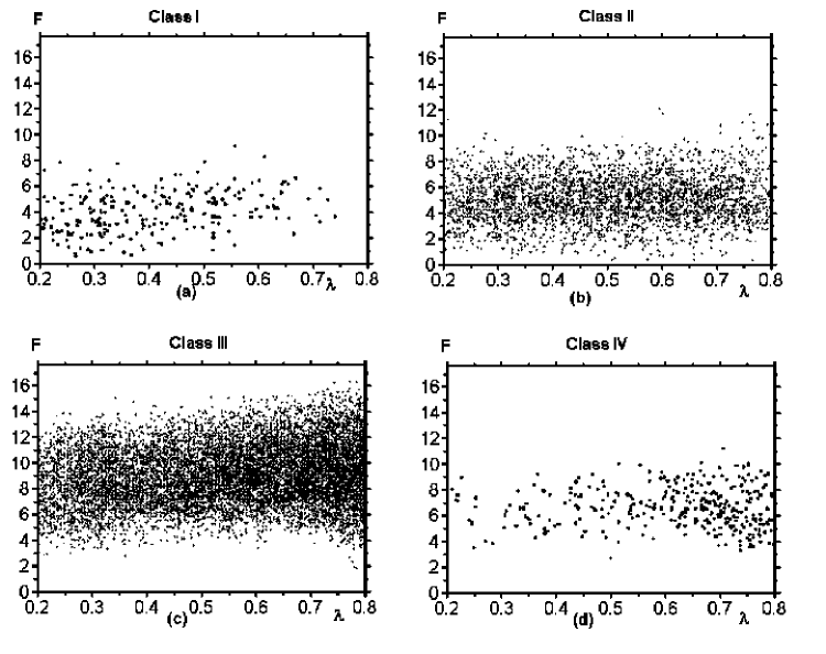
Figure 3: Distribution of rule tables in ($\lambda$,F) plane. Fig. 3(a): The distribution of 483 class I rule tables. Fig. 3(b): The distribution of 3169 class II rule tables. Fig. 3(c): The distribution of 10248 class III rule tables. Fig. 3(e): The distribution of 329 class IV rule tables.

The Figs. 3 shows that the class III rule tables are located in the larger $F$ region; about $F\geq 4$, while class I, class II rule tables, in the smaller $F$ region; about $F\leq 9$, and the class IV rule tables are found in the overlap region of class II and class III rule tables; about $4\leq F\leq 9$. These results support the chaotic limit and periodic limit discussed in the subsection III B, and shows that at least in the $0.2\leq\lambda\leq 0.75$ range, all four pattern classes coexist.
These distributions of rule table in $F$, are almost independent of $\lambda$. It means that the CA pattern classes are not classified by $\lambda$, contrary to the results of Ref. langton , but are classified rather well by the quiescent string dominance parameter $F$.
Let us discuss the reason why Langton had obtained his results. If the rule tables are generated using the probability $\lambda$ by the ”random-table method” or ”random-walk-through method”langton , the numbers of the group 1 rule tables $N_{4}$, $N_{3}$, $N_{2}$ and $N_{1}$ are also controlled by the probability $\lambda$. They distribute around $N^{\lambda}_{i}$ of section IV. Then the $F$ parameters are also distributed around,

$$F^{\lambda}=(6+33r_{3}+72r_{2}+144r_{1})\lambda.$$ (15)

Therefore in these methods, $\lambda$ and $F$ are strongly correlated. The probabilities to obtain the rule tables, which are far apart from the line given by Eq. (15) are very small. When $\lambda$ is small, the rule table with small $F$ are mainly generated, which are class I and class II CAs. On the other hand in the large $\lambda$ region, the rule tables with large $\lambda$ are dominantly generated, which are class III CAs. The line of Eq. (15) crosses the location of class IV pattern classes around $0.4\leq\lambda\leq 0.55$. This might be a reason Langton has obtained his results. But the distribution of rule tables in all ($\lambda$,F) plane, show the global structure of the CA rule table space as in Fig. 3 and lead us to deeper understanding of the structure of CA rule tables.
We should like to stress again that four pattern classes do coexist in a rather wide range in $\lambda$, which are rather well classified by the parameter $F$ not by $\lambda$.

VI Classification of Rule tables in ($\lambda$,F) Plane

In the Fig. 3, it is found that rule tables are not separated by sharp boundaries. And they seem to have some probability distributions. We denote the probability densities of class I, class II, class III and class IV pattern classes as $P^{I}$, $P^{II}$, $P^{III}$ and $P^{IV}$, respectively and proceed to classify the rule tables by using them.
The equilibrium points $F^{II-III}_{E}(\lambda)$ of class II and class III rule tables are defined by the point where the relation $P^{II}(F)=P^{III}(F)$ is satisfied. The region in ($\lambda$,$F$) plane where $P^{II}$ and $P^{III}$ coexist in a similar ratio is defined as transition region. The upper points of the transition region $F^{II-III}_{U}$, are defined by the points, $P^{II}$=$\frac{P^{III}}{e}$ and similarly for the lower points of the transition region $F^{II-III}_{L}$, where $P^{II}$ and $P^{III}$ are interchanged. By these three points, $F^{II-III}_{E}$, $F^{II-III}_{U}$ and $F^{II-III}_{L}$, we define the phase boundary of the rule tables.
The distributions of the rule tables in the Fig. 3 show the qualitative probability distributions. However in order to study the $\lambda$ dependences of $F^{II-III}_{E}$, $F^{II-III}_{U}$ and $F^{II-III}_{L}$ more quantitatively, we generate a rule tables at fixed $\lambda$s. The $\lambda$ points and numbers of the rule tables are shown in Table 5.

Table 5: The data points, numbers of each pattern classes and the transition parameters of CA(5,4). The column ”Comp” shows the numbers of rule tables which transmit the information of initial states.

		Number of the rule tables					Class I - II			Class II - III
$\lambda$	$N_{h}$	I	II	III	IV	Comp	$F^{I-II}_{L}$	$F^{I-II}_{E}$	$F^{I-II}_{U}$	$F^{II-III}_{L}$	$F^{II-III}_{E}$	$F^{II-III}_{U}$
$0.125$	128	202	1081	1052	42	16	0.0	2.0	3.2	3.0	6.6	9.0
$0.15$	154	99	499	545	23	17	0.7	2.0	3.6	3.5	6.5	9.1
$0.2$	205	141	728	1021	39	18	1.2	2.0	3.6	4.7	6.3	8.5
$0.25$	256	98	479	949	19	8	0.0	1.7	3.8	4.4	5.9	7.5
$0.3$	307	83	364	878	13	6	1.2	2.0	3.9	4.0	6.0	7.3
$0.4$	410	117	385	1169	23	7			3.7	4.5	5.7	7.0
$0.5$	512	53	341	884	23	7				4.8	6.0	7.2
$0.6$	615	38	488	1316	61	10				4.8	6.1	7.3
$0.7$	717	4	333	974	89	7				4.9	5.8	6.8
$0.75$	768	2	256	960	108	7				4.5	5.4	6.6
$0.8$	819	2	81	1064	12	5						4.3

At each fixed $\lambda$, we divide the region in $F$ into bin sizes of $\delta F=1$, and count the number of rule tables of each classes in these bins. From these results, we estimate the probability densities $P(F_{i})$, where $F_{i}$ is a middle point of that bin.
Let us proceed to the classification of the class II and class III rule tables.

VI.1 Classification of rule tables in $\frac{1}{4}\leq\lambda\leq 1-\frac{1}{4}$

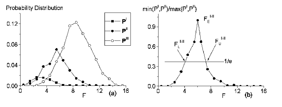
Figure 4: The probability distributions $P^{I}$, $P^{II}$ and $P^{III}$ and determination of $F^{II-III}_{E}$, $F^{II-III}_{L}$ and $F^{II-III}_{U}$ at $\lambda=0.3$. Fig. 4(a): $P^{I}$, $P^{II}$ and $P^{III}$ distributions. Fig. 4(b): An example of the determination of $F^{II-III}_{E}$, $F^{II-III}_{L}$ and $F^{II-III}_{U}$.

.

The probability distributions of $P^{II}(F)$ and $P^{III}(F)$ at $\lambda=0.3$ are shown in Fig. 4(a), and the determination of the $F^{II-III}_{E}$, $F^{II-III}_{U}$ and $F^{II-III}_{L}$ are demonstrated in Fig. 4(b). For the other $\lambda$ points of Table 5, $F_{E}$, $F_{U}$ and $F_{L}$ are determined in the similar way. They are summarized in the Table 5.
As already seen in Fig. 3, the $\lambda$ dependences of the $F^{II-III}_{E}$, $F^{II-III}_{U}$ and $F^{II-III}_{L}$ are small, in the region $0.25\leq\lambda\leq 0.75$. This is also confirmed by the studies at fixed $\lambda$s as shown in in the Table 5.

VI.2 Classification of rule tables in larger and smaller $\lambda$ region

The $P^{II}$ and $P^{III}$ at $\lambda=0.8$ are shown in Fig. 5.

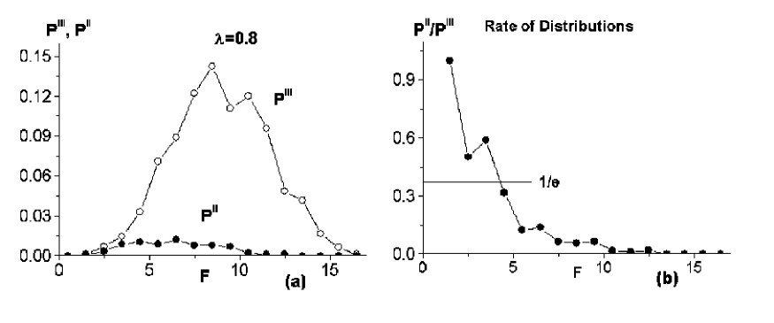
Figure 5: The probability distributions $P^{II}$ and $P^{III}$ and the determination of $F^{II-III}_{E}$, $F^{II-III}_{L}$ and $F^{II-III}_{U}$ at $\lambda=0.8$. Fig. 5(a) shows $P^{II}$ and $P^{III}$. In Fig. 5(b), it is found that $F^{II-III}_{E}$, $F^{II-III}_{L}$ could not be obtained.

It should be noticed that there is no region of $F$ where $P^{II}\geq P^{III}$. This means that $F^{II-III}_{E}$ and $F^{II-III}_{L}$ disappears. Only $F^{II-III}_{U}$ is determined.
In order to understand what has changed at $\lambda=0.8$, we have studied the $\lambda$ dependences of $P^{II}$ and $P^{III}$ in the region $\lambda\geq 0.7$. They are shown in Fig. 6.

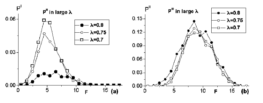
Figure 6: The $\lambda$ dependences of $P^{II}$ and $P^{III}$ in the region, $\lambda\geq 0.7$

It is found that $P^{III}$ gradually increases as $\lambda$ becomes larger but the increase is quite small, while $P^{II}$ decreases abruptly between $\lambda=0.75$ and $\lambda=0.8$. As a result $P^{II}$ becomes less than $P^{III}$ in all $F$ regions. This tendency could already be observed in Fig. 3(b), but it is quantitatively confirmed by the studies at fixed $\lambda$s.
In the smaller $\lambda$ region ($\lambda\leq 0.3$), the behavior of $P^{II}$ and $P^{III}$ are shown in Fig. 7. In this case, $P^{II}$ is gradually increasing as $\lambda$ decreases but the change is small. On the contrary, the decrease in $P^{III}$ is larger. As a consequence of these changes the transition region of the class II and class III pattern classes spread over wider range in $F$.

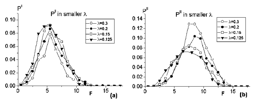
Figure 7: The $\lambda$ dependences of $P^{II}$ and $P^{III}$ in the region, $\lambda\leq 0.3$

These results are also summarized in Table 5 and shown in Fig. 8.
In the same way, the classification of the class I and class II rule tables could be carried out. The preliminary results are shown in the column $F^{I-II}_{E}$, $F^{I-II}_{U}$ and $F^{I-II}_{L}$ of the Table 5. In this case too, it is seen in Fig. 3(a), (b) that density of class I rule tables decreases as $\lambda$ increases, while that of class II rule tables stays almost constant in $\lambda\leq 0.75$. This feature is more quantitatively confirmed by the studies at fixed $\lambda$s. At $\lambda=0.4$, there disappears the region of $F$, where $P^{I}$ is larger than $P^{II}$ and $F^{I-II}_{L}$ and $F^{I-II}_{E}$ could not be determined, just as in the same way as $P^{II}$ and $P^{III}$ distributions at $\lambda=0.8$. These results are also shown in Table 5.
However we should like to say that the numbers of the class I rule tables, and those of class II rule tables in the region $F\leq 3$ are not large. Therefore the results may suffer from large statistical fluctuations. We think that the classification of class I and class II rule table needs more data to get quantitative conclusions, however the qualitative properties will not be changed.

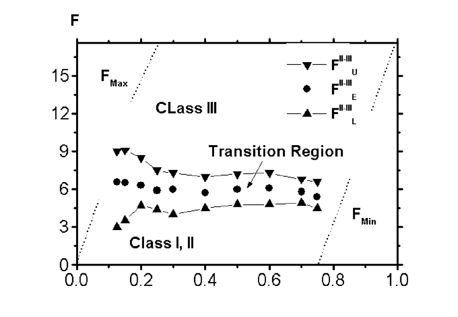
Figure 8: The phase diagram of CA(5,4). The minimum of $F$ ($F_{Min}$) and the maximum of $F$ ($F_{Max}$), which are discussed at the end of subsection VI B, are shown by the dotted lines.

We proceed to the investigation of the classification of rule tables outside of these $\lambda$ region. In $\lambda<0.25$ region, not all the group 2 rules could be replaced by the group 1 rules. Therefore the maximum numbers of group 1 rules $N(g1)_{Max}$ could not become 256, and it decreases to zero as $\lambda$ approaches to zero. Then the maximum of $F$, ($F_{Max}$) also decreases to zero toward $\lambda=0$.
Conversely in $\lambda>0.75$ region, not all the group 1 rules could be replaced by the group 2 rules. The minimum of N(g1) and therefore the minimum of $F$, ($F_{Min}$) could not becomes 0. The line $F_{Min}$ increases until its maximum at $\lambda=1$. In Fig. 8, we have schematically shown the $F_{Max}$ and $F_{Min}$ lines with dotted lines. We should like to stress that the dotted line should have some width due to fluctuations of $N_{4}$, $N_{3}$, $N_{2}$ and $N_{1}$ caused by the randomness.

VII Discussions and Conclusions

VII.1 Transmission of initial state informations

The computability of the CA is discussed very precisely mainly for elementary CA (CA(3,2)) in series of paper from Santa Fe Institutehanson . In this subsection we discuss on the simplest problem of transmission of the initial state information to the later configurations.
We have found some examples where class II and class IV patterns appear with similar probability by changing the initial configurations randomly. An example is shown in the Fig. 9, which is the transmission of initial state information to later configurations and is similar to the $\rho=1/2$ problem in the CA(3,2). It is interesting to investigate under what condition the changes of the pattern classes are taken place.

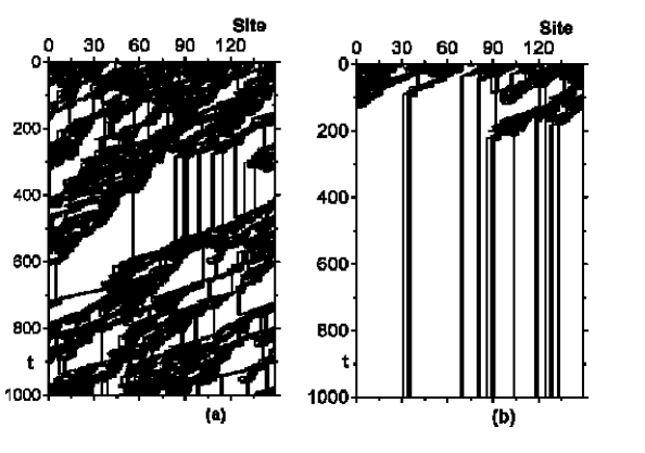
Figure 9: An example of the transmission of the initial state information at $\lambda=0.75$. Fig. 9(a), and Fig. 9(b) are generated by the same rule table. Only the difference is the initial states configurations which are set randomly.

We have focus on the difference of patten classes between class II and class IV, because in this case differences of the patterns are obvious. These rule tables are found in the wide region in $\lambda$, $0.125\leq\lambda\leq 0.8$. The numbers of the rule tables of this property at fixed $\lambda$s are also shown in the column ”Comp” of Table 5.
In addition, there are cases where the difference of patters seems to be realized within the same pattern classes. In these cases careful studies are necessary to distinguish the difference of these patterns. In this article, we have not studied these cases.

VII.2 Classification of rule table by the intuitive $F$ parameter

The methods to determine the coefficients $r_{i}$ in Eq. (11) are not unique. In the section IV, in order to determine them we have used regression hyper plane of class IV rule tables, and in order to obtain 329 class IV rule tables, we have generated totally about 14000 rule tables. It is a rather tedious task. However optimal set of $r_{i}$ has been close to the intuitive set of $r_{i}$.
In this subsection we study the classification of rule tables by the intuitive $F$ parameter. The same analyses as sections V and VI are carried out and as the similar figures are obtained in this case too, we will show only the distributions of the rule tables in ($\lambda$,F) plane in Fig. 10.

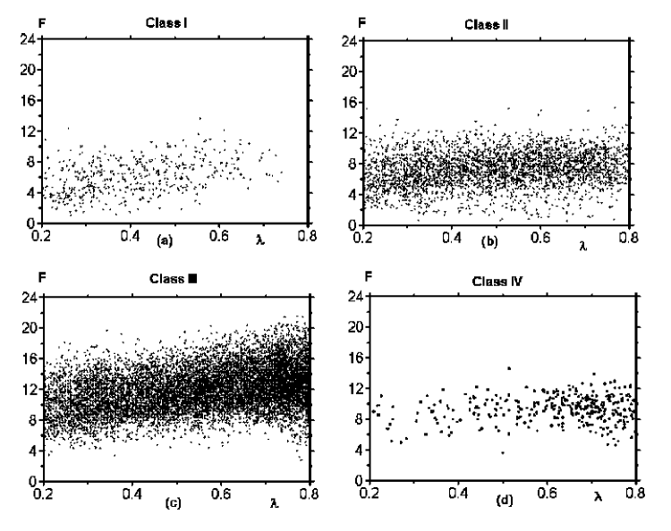
Figure 10: The distribution of rule tables by using intuitive $F$ parameter. The numbers of the data points are same as in the case of Fig.3.

The Figs. 10 are very similar to the Figs. 3. Therefore the classification of the rule table space are almost same as Fig. 8, except that the $F_{Max}$ changes from 17.6 to 24.
If intuitive $F$ parameter could successfully classify the rule tables for general CA(N,K) it would be very convenient, because it reflect the structure of the CA rules and there is no need to gather a lot of class IV rule tables, in order to determine $r_{i}$s. Whether it is correct or not must be concluded after the studies of other CA(N,K).

VII.3 Conclusions and discussions

We have started to find the mechanism which distinguishes the pattern classes at same $\lambda$s, and have found that it is closely related to the structure of the rule tables. The patten classes of the CA are mainly controlled by the numbers of the group 1 rules, which has been denoted by $N(g1)$.
In the CA(N,K),in the region $\frac{1}{K}\leq\lambda\leq 1-\frac{1}{K}$, the maximum of $N(g1)_{Max}$ corresponds to a chaotic limit, and its minimum $N(g1)=0$, to a periodic limit. Therefore in this $\lambda$ region, we could control the patten classes by changing $N(g1)$ without fail. The method for it is the replacements of Eq. (LABEL:eq:del_num_RP). Using the replacements, we could study the rule tables which are difficult to obtain by the ”random-table method” or ”random-walk-through method” of Ref.langton . This property could be studied quantitatively by introducing a quiescent string dominance parameter $F$.
In this article, a quantitative studies are carried out for CA(5,4). In this case, the group 1 rules are further classified into 5 types as shown in Table 1, and the classification of rule tables is carried out in ($\lambda$,F) plane as shown in Fig. 8. It is seen that the $\lambda$ dependences of the transition region are very gentle, and rule tables are classified better by the $F$ parameter rather than by $\lambda$. It is interesting whether or not the $\lambda$ dependences of the transition region depend on the models.
In the replacement experiments, we have found the edge of chaos (very long transient lengths) behavior in many cases. The examples are shown in Fig. 2. Sometimes they are observed in some range in $N_{3}$ or $N_{2}$. This indicates that in many cases, the transitions are second-order like. But the widths in the ranges of $N_{3}$ or $N_{2}$ are different from each other, and there are cases where the widths are less than one unit in the replacement of RP2 (first-order like). It is very interesting to investigate under what condition the transition becomes first-order like or second-order like. The mechanism of the difference in the transitions is an open problem and it may be studied by taking into account effects of group 3 and 4 rules. In these studies another new parameters might be found and a more quantitative phase diagram might be obtained.
These issues together with finding the points where the transition region crosses $F_{Max}$ and $F_{Min}$ lines (dotted lines) in Fig. 8, and the nature of the transition at these points will be addressed in the forthcoming publications.

References

- (1) S. Wolfram, Physica D 10(1984) 1-35.
- (2) S. Wolfram, Physica Scripta T9(1985) 170-185.
- (3) C.G.Langton, Physica D 42(1990) 12-37.
- (4) J.E.Hanson and J.P.Crutchfield, Physica D 103(1997),169-189, and references therein.
- (5) A. Wuensche, Complexity Vol.4(1999) 47-66.
- (6) P.M. Binder Complex System 7(1993),241-247
- (7) G.M.B.Oliveira, P.P.B.de Oliveira, Nizam Omar Artificial Life 7(2001),277-301
- (8) N.H.Packard, Adaption toward the edge of chaos. In ”Dynamic Patterns in Complex System”(1988), 293-301, edited by J. A. S. Kelso, A. J. Mandel,and M. F. Shlesinger,World Scientific,Singapore.
- (9) M. Mitchell, J.P.Crutchfield and P.T. Hraber, Santa Fe Institute Studies in the Science of Complexity, Proceedings Volume 19. Reading, MA:, Addison-Wesley. online paper, http://www.santafe.edu/ mm/ paper-abstracts.html#dyn-comp-edge.
- (10) C.G.Langton, Physica D 22(1986) 120-149.
- (11) W.LI, N.H.Packard and C.G.Langton, Physica D45(1990) 77-94.
-
(12)
T. Suzudo, Crystallisation of Two-Dimensional
Cellular Automata, Complexity International, Vol. 6(1999).
on line journal,
http://www.csu.edu.au/ci/vol06/suzudo/suzudo.html. See appendix.