A Test of a Test for Chaos

Abstract

A simple new binary test for chaos has been proposed by Gottwald and Melbourne. We apply this test successfully to the Henon-Heiles and Lorenz systems, demonstrating its applicability to conservative systems, as well as dissipative systems. The binary test is effective for highly chaotic Hamiltonian systems and orbits on a strange attractor and is particularly useful as a marker of the transition from regularity to chaos. However, we find it is not able to detect more subtle instances of transient chaos.

PACS 05.45.-a,82.40.Bj ]

I Introduction

A promising new binary test for chaos has been proposed by Gottwald and Melbourne [1]. The test returns 0 for a non-chaotic system and 1 for a chaotic system. It does not offer any quantitative information and so cannot quantify the degree of irregularity in the way a Lyapunov exponent might. However, it can provide a quick and useful diagnostic for chaos.

Consider a base dynamical system ${\bf\dot{x}}={\bf f}({\bf x})$ of any dimension with orbits ${\bf x}(t)$. The proposed method to determine if it is chaotic is based on a Euclidean ${\bf E}(2)$ group extension of the underlying base dynamics [3, 4]. The dynamics is explicitly extended to include two new variables $(p,q)$ defined through

$$\dot{p} = \phi({\bf x})\cos(\omega_{0}t),$$ (1)

$$\dot{q} = \phi({\bf x})\sin(\omega_{0}t),$$ (2)

where $\phi({\bf x})$ is any observable of the base dynamics and $\omega_{0}\neq 0$ is an arbitrary constant frequency that is needed to damp off any linear growth that may be common to both non-chaotic and chaotic orbits. If the observable $\phi$ is drawn from a non-chaotic system, then the $(p,q)$ subspace will be bounded. But if the observable $\phi$ is drawn from a chaotic system, then the motion in the $(p,q)$ subspace will be Brownian and unbounded. The extended variables diffuse through the subspace as the observables of the base dynamics jump around unpredictably.

Gottwald and Melbourne introduced a binary test for chaos by defining a mean-square displacement

$$M(t)=\lim_{T\rightarrow\infty}{\frac{1}{T}}\int_{0}^{T}\left(p(t+\tau)-p(\tau)\right)^{2}d\tau$$ (3)

and characterizing the behaviour of $M(t)$ through

$$K=\lim_{t\rightarrow\infty}{\frac{\log M(t)}{\log t}}\ \ .$$ (4)

If there is no chaos then the motion in $p(t)$ is bounded and $K\rightarrow 0$. If the base dynamics is chaotic then $p(t)$ will exhibit Brownian diffusion so that $\Delta p\rightarrow t^{1/2}$ as $t\rightarrow\infty$ and $K\rightarrow 1$. The $K$-test can be used for both continuous and discrete dynamical systems even when the precise underlying base dynamics is unknown [1].

This test has certain advantages of simplicity and was shown to confirm the results of testing for chaos using Lyapunov exponents for the forced van-der-Pol system [1]. We show here that the $K$-test also confirms the trend of the Lyapunov exponents for the simple Hamiltonian system of Henon and Heiles [2]. So the $K$-test is applicable to Hamiltonian as well as dissipative systems.

While the test works well as a diagnostic of the transition from regularity to chaos we express some reservations about the use of the test on an orbit by orbit basis. Most importantly, we found the method difficult to interpret for systems that experienced chaotic transients in contrast to the easy interpretation of dissipative systems near a strange attractor, or in highly chaotic Hamiltonian systems. To illustrate this we use the Lorenz model [5] to show that transient chaos, which can be found in the Lorenz system by other means, goes undetected by the $K$-test. Orbits that enter highly chaotic regions of phase space and then depart into regular regions are not Anosov and may not show the diffusive motion in phase space required to yield a $K\rightarrow 1$ result from the test. These transient systems may not satisfy the criteria for a system within the remit of the $K$-test. This signals one of the possible limitations of the K-test.

II Henon-Heiles

The Henon-Heiles system is an ideal Hamiltonian system on which to evaluate the utility of the $K$-test. It provides a simple and well understood model for the motion of stars in a galactic potential as well as for the motion of non-linearly-coupled molecules. The transition from regularity to chaos as the energy is increased is well documented and can be identified with Poincaré surfaces of section, Lyapunov exponents, and the Painlevé property.

The Henon-Heiles Hamiltonian is

$$H={\frac{1}{2}}\left(p_{x}^{2}+p_{y}^{2}+x^{2}+y^{2}\right)+x^{2}y-{\frac{1}{3}}y^{3}$$ (5)

with equations of motion

$$\dot{x} = p_{x}$$ (6)

$$\dot{y} = p_{y}$$ (7)

$$\dot{p}_{x} = -x-2xy$$ (8)

$$\dot{p}_{y} = -y-x^{2}+y^{2}\ \ .$$ (9)

We add the Euclidean extension

$$\dot{p} = x\cos(\theta)$$ (10)

$$\dot{q} = x\sin(\theta)$$ (11)

$$\dot{\theta} = \omega_{0}$$ (12)

where we have chosen $\phi=x$. We evolve these equations numerically and check that the Hamiltonian remains conserved throughout the simulation. Our results are summarized in Figs. 1 and 2. The orbits selected for display have identical initial conditions up to the energy $H$ which was varied from orbit to orbit. The value of $K(t)$ is measured as the slope of the line $ln(M(t))$ versus $ln(t)$ and is plotted in Fig. 1 as a function of the energy $H$. The transition from non-chaotic orbits ($K\rightarrow 0$) to chaotic orbits ($K\rightarrow 1$) as the energy increases is clearly demonstrated. The transition confirms the break up of tori in the phase space for the base dynamics (and therefore the non-integrability of the base dynamics) as the energy grows. We also confirm the onset of chaotic motion for these orbits with a numerical determination of the principal Lyapunov exponent shown as a function of $H$ in Fig. 2.

FIG. 1.: The asymptotic value of $K$ versus the energy $H$ for the Henon-Heiles system.

FIG. 2.: The asymptotic value of the principal Lyapunov exponent versus the energy $H$ for the Henon-Heiles system.

A few comments on Fig. 1 should be made. The convergence of the value of $K$ towards either $0$ or $1$ can be improved if the numerical simulations are allowed to run far longer and a more precise extrapolation method is used so as to avoid any early transients. Of course, this renders the application more numerically intensive and slower without yielding a very great improvement in convergence. There is also a clear dependence of the motion in the Euclidean subspace on the specific value of $\omega_{0}$ employed. However, the overall trend in $K$ is typically the same for various values of $\omega_{0}$.

While Fig. 1 does show the required transition from 0 to 1, it is important to stress how the conservative system differs from the dissipative system. For a dissipative system all trajectories, regardless of initial conditions, are drawn onto the same attractor. Therefore the $K$-test should show no dependence on initial conditions. This is not true for a Hamiltonian system. There can be a mixture of regular and irregular orbits and so the test result can depend on initial conditions. Only for a completely ergodic system will $K\rightarrow 1$ independent of initial conditions. Also, since chaotic transients can often arise in conservative systems, the $K$-test may not always give such a crisp transition. Chaotic transients in dissipative systems are discussed further in the next section.

III Lorenz

The standard Lorenz system demonstrates a transition from no chaos to transient chaos and then further to a full chaotic attractor. The standard system is

$$\dot{X} = -\sigma(X-Y),$$ (13)

$$\dot{Y} = -XZ+rX-Y,$$ (14)

$$\dot{Z} = XY-bZ,$$ (15)

with $\sigma=10$ and $b=8/3$ and we vary the constant $r$. The transition to chaos is summarized in Ref. [6]. For $r<1$ there is one fixed point at $X=Y=Z=0$ and no chaos. For $1<r\mathrel{\hbox to0.0pt{\lower 3.0pt\hbox{$\mathchar 536\relax$}\hss}\raise 2.0pt\hbox{$\mathchar 316\relax$}}13.96$ there are two additional attractors, one at

$$X_{R} = (b(r-1))^{1/2}$$ (16)

$$Y_{R} = (b(r-1))^{1/2}$$ (17)

$$Z_{R} = r-1,$$ (18)

and another at $(X_{L},Y_{L},Z_{L})=(-X_{R},-Y_{R},Z_{R}),$ but still no chaos. A non-chaotic orbit drawn onto the simple fixed point $(X_{R},Y_{R},Z_{R})$ with $(\dot{X},\dot{Y},\dot{Z})\rightarrow 0$ is shown in Fig. 3. A closely neighbouring orbit will follow a similar path onto the same attractor since there is no exponential sensitivity to initial conditions, no positive Lyapunov exponent, and no chaos.

However, for values of $r\mathrel{\hbox to0.0pt{\lower 3.0pt\hbox{$\mathchar 536\relax$}\hss}\raise 2.0pt\hbox{$\mathchar 318\relax$}}13.96$ a non-attracting form of transient chaos develops around a homoclinic orbit in phase space, first noted by Kaplan and Yorke [7]. Two orbits undergoing transient chaos are shown in Fig. 4. One orbit winds around a bit before being drawn onto the regular attracting point $(X_{L},Y_{L},Z_{L})$ while its very near neighbour ends up on $(X_{R},Y_{R},Z_{R})$.

FIG. 3.: A nonchaotic orbit for $r=10$ being drawn onto the regular attracting fixed point at $(X_{R},Y_{R},Z_{R})$. The orbit began with initial conditions $X(0)=1.99895$, $Y(0)=0$, and $Z(0)=9.99005$.

FIG. 4.: An orbit in the $(X,Z)$ plane with $r=18$ exhibiting transient chaos before gliding towards the (not strange) attractor at $(X_{L},Y_{L},Z_{L})$. Left: The orbit began with initial conditions $X(0)=1.99885$, $Y(0)=0$, and $Z(0)=9.99005$. Right: A neighbouring orbit with $X(0)=1.99895$, $Y(0)=0$, and $Z(0)=9.99005$ is drawn onto the other regular attractor at $(X_{R},Y_{R},Z_{R})$.

We choose to use the method of fractal basin boundaries to locate regions of transient chaos. An initial slice in phase space is color-coded according to whether the orbit eventually lands on the fixed point $(X_{R},Y_{R},Z_{R})$ (black) or the fixed point $(X_{L},Y_{L},Z_{L})$ (white). In the absence of chaos all the basins will have smooth boundaries. In the presence of chaos the boundaries become fractal, demonstrating both extreme sensitivity to initial conditions and a chaotic mixing of orbits. Such fractal basin boundaries are illustrated in Fig. 5; the orbits shown in Fig. 4 are drawn from along the fractal. They have nearly identical initial values but divergent outcomes, a characteristic of chaotic transients.

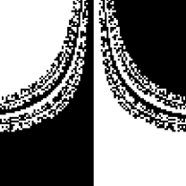
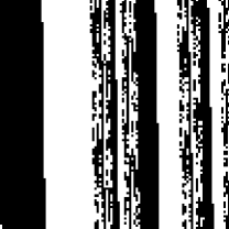
FIG. 5.: Upper Figure: A fractal basin boundary in $(X,Z)$ for $r=18$. The range of initial conditions is $-10\leq X(0)\leq 10$ and $0\leq Z(0)\leq 10$ while for all orbits $Y(0)=0$. Middle Figure: A detail of the fractal basin boundary in $(X,Z)$. The range of initial conditions is $1\leq X(0)\leq 2$ and $9.9\leq Z(0)\leq 10$ while again $Y(0)=0$. Lower Figure: A detail of the detail. The range of initial conditions is $1.99\leq X(0)\leq 2$ and $9.99\leq Z(0)\leq 10$ with $Y(0)=0$.

FIG. 6.: An orbit in the $(X,Z)$ plane along the strange attractor for $r=30$. The orbit began with initial conditions $X(0)=1.99895$, $Y(0)=0$, and $Z(0)=9.99005$.

For $r\mathrel{\hbox to0.0pt{\lower 3.0pt\hbox{$\mathchar 536\relax$}\hss}\raise 2.0pt\hbox{$\mathchar 318\relax$}}24.06$ the transient chaos gives way to chaos on attractors which merge into the famous Lorenz strange attractor beyond $r\mathrel{\hbox to0.0pt{\lower 3.0pt\hbox{$\mathchar 536\relax$}\hss}\raise 2.0pt\hbox{$\mathchar 318\relax$}}24.74$ [6]. An orbit that drifts onto the strange Lorenz attractor is shown in Fig. 6.

We apply the $K$-test to the Lorenz system and show that it effectively marks the transition from non-chaotic motion to chaos on a strange attractor at $r\simeq 24.74$ where we see $K$ rising from $0$ to $1$. However, the test is unable to pick up the chaotic transient behaviour for values of $13.96\mathrel{\hbox to0.0pt{\lower 3.0pt\hbox{$\mathchar 536\relax$}\hss}\raise 2.0pt\hbox{$\mathchar 318\relax$}}r\mathrel{\hbox to0.0pt{\lower 3.0pt\hbox{$\mathchar 536\relax$}\hss}\raise 2.0pt\hbox{$\mathchar 318\relax$}}24.06$. Notice that a similar random scan through the Lyapunov exponents in Fig. 8 also misses the transient episodes although short time exponents along the fractal basin boundary can be isolated.

FIG. 7.: The asymptotic value of $K$ versus the parameter $r$ for orbits with inital values $X(0)=1.99895$, $Y(0)=0$, and $Z(0)=9.99005$.

FIG. 8.: The principal Lyapunov exponent versus the parameter $r$ for orbits with inital values $X(0)=1.99895$, $Y(0)=0$, and $Z(0)=9.99005$.

Specific orbits of Fig. 7 can be isolated to illustrate the behaviour in the $(p,q)$ subspace explicitly. The orbit at $r=18$ corresponds to the right-most orbit in Fig. 4. The orbit winds around before drifting onto the fixed point $(X_{R},Y_{R},Z_{R})$. This is reflected in the $(p,q)$ subspace by the stray steps taken before the orbit moves onto the smooth, bounded ring of the regular attractor as shown in Fig. 9. This results in a regular oscillation in the mean-square displacement $M(t)$ that will eventually die away to give $K\rightarrow 0,$ as shown in Fig. 7. The $K$-test reflects the regularity of the attractor and is unable to detect the subtle chaotic transient in the early motion.

FIG. 9.: The bounded regularity of the $(p,q)$-extension for an orbit sampled from Fig. 7. The orbit corresponds to $r=18$ with inital values $X(0)=1.99895$, $Y(0)=0$, and $Z(0)=9.99005$ (see Fig. 4).

By contrast, an orbit at $r=30$ in Fig. 7 is drawn onto the Lorenz strange attractor and its strongly chaotic behaviour is detected by the $K$-test. The chaotic motion is well reflected by the Brownian diffusion evidenced in the $(p,q)$ subspace shown in Fig. 10. This orbit leads to $K\rightarrow 1$ as expected.

FIG. 10.: The figure shows the unbounded Brownian like diffusion of the $(p,q)$-extension for a chaotic orbit for which $K\sim 1$ in Fig. 7. The orbit corresponds to $r=30$ with inital values $X(0)=1.99895$, $Y(0)=0$, and $Z(0)=9.99005$ and moves onto the Lorenz strange attractor.

IV Summary

We have confirmed that the $K$-test provides a simple and easy diagnostic for the transition from regularity to chaos for Hamiltonian as well as dissipative systems. For the test to be effective, an orbit must spend sufficient time on the hyperbolic chaotic attractor in a dissipative system, or be confined to a highly chaotic region of phase space if the system is Hamiltonian. However, for chaotic transients which move into a chaotic region of phase space and then out into a regular region of phase space the motion is not consistently Brownian. Consequently, the test can yield ambiguous and confusing results although a qualitative look over the $(p,q)$ subspace can provide guidance as to the transient irregularity of the base dynamics. Additionallly the K-test is not ideal for relativistic settings since it depends on the time coordinate used and so, like the Lyapunov exponents, is not a covariant indicator of chaos. These limitations of the $K$-test are not unexpected: no one probe of chaos can suit every scenario. Nor are they fatal to its utility. Rather, we hope that they will help to map out the territory over which this simple test is a reliable guide to the presence of chaos

REFERENCES

- [1] G. A. Gottwald and I. Melbourne, nlin.CD/0208033.
- [2] M. Henon and C. Heiles, Ap. J. 69 73 (1964).
- [3] M. Nicol, I. Melbourne, and P. Ashwin, Nonlinearity 14 275 (2001).
- [4] M.J. Field, I. Melbourne, and A. Török, Ergod. Th. & Dynam. Sys. in press (2002).
- [5] E. Lorenz, J. Atmos. Phys. 20 130 and 148 (1963).
- [6] E. Ott, Chaos in dynamical systems, (Cambridge University Press, Cambridge, 1993).
- [7] J.J. Kaplan and J.A. Yorke, Comm. Math. Phys. 67 93 (1979).