Synchronized clusters in coupled map networks: Stability analysis

Abstract

We study self-organized (s-) and driven (d-) synchronization in coupled map networks for some simple networks, namely two and three node networks and their natural generalization to globally coupled and complete bipartite networks. We use both linear stability analysis and Lyapunov function approach for this study and determine stability conditions for synchronization. We see that most of the features of coupled dynamics of small networks with two or three nodes, are carried over to the larger networks of the same type. The phase diagrams for the networks studied here have features very similar to the different kinds of networks studied in Ref. sarika-REA2 . The analysis of the dynamics of the difference variable corresponding to any two nodes shows that when the two nodes are in driven synchronization, all the coupling terms cancel out whereas when they are in self-organized synchronization, the direct coupling term between the two nodes adds an extra decay term while the other couplings cancel out.

I Introduction

Recently it has been observed that several complex systems have underlying structures that are described by networks or graphs having interesting properties Strogatz ; rev-Barabasi . Many of these naturally occurring large and complex networks come under some universal classes and they can be simulated with simple mathematical models, viz small-world networks Watts , scale-free networks scalefree etc. These models are based on simple physical considerations and have attracted a lot of attention from physics community as they give simple algorithms to generate graphs which resemble actual networks found in many diverse systems such as the nervous systems koch , social groups social , world wide web www , metabolic networks metabolic , food webs food and citation networks citation .

Several networks in real world consist of dynamical elements interacting with each other and they have large number of degrees of freedom. Synchronization in dynamical systems with many degrees of freedom has attracted much attention in recent decades book1-syn ; book2-syn . In Refs. sarika-REA1 ; sarika-REA2 two of us have presented detailed analysis and numerical results of phase synchronization and cluster formation in coupled maps on different networks. Starting from random initial conditions the asymptotic behaviour of these coupled map networks (CMNs) has revealed that there are two different mechanisms leading to two types of synchronized clusters. First there are clusters with dominant intra-cluster couplings which are referred as self-organized (s-) synchronization and secondly there are clusters with dominant inter-cluster coupling which are referred as driven (d-) synchronization sarika-REA1 ; sarika-REA2 . The numerical studies reveal several clusters with both types as well as clusters of mixed type where both mechanisms contribute. There are also situations where ideal clusters of both types are observed. An analysis of simple networks with two and three nodes indicates that the self-organized behaviour has its origin in the decay term arising due to intra-cluster couplings in the dynamics of the difference variables while the driven behaviour has its origin in the cancellation of the inter-cluster couplings in the dynamics of the difference variables.

In the present paper we study the dynamics of some simple networks analytically and numerically with a view to get a better understanding of the two mechanisms of cluster formation discussed above. Mainly we study the asymptotic stability of s- and d-synchronization in networks with small number of nodes, i.e. two and three nodes, and extension of these small networks to networks with large number of nodes. As an example of large networks showing s-synchronized clusters we take globally coupled maps kaneko-GCM and for d-synchronized clusters we take complete bipartite coupled maps bi-partite .

The paper is organized as follows. In Section II, we state the model and discuss general features of the stability of synchronized states. Section III discusses two networks showing s-synchronization, i.e. two nodes network and globally connected network. Section IV considers two networks showing d-synchronization, i.e. three nodes bipartite network and complete bipartite network. Section V concludes the paper.

II Model of a coupled map network (CMN)

Consider a network of $N$ nodes and $N_{c}$ connections (or couplings) between the nodes. Let each node of the network be assigned a dynamical variable $x^{i},i=1,2,\ldots,N$. The dynamical evolution of coupled maps can be written as sarika-REA2

$$x^{i}_{t+1}=(1-\epsilon)f(x^{i}_{t})+\frac{\epsilon}{k_{i}}{\sum_{j=1}^{N}C_{ij}g(x^{j}_{t})}$$ (1)

where $x^{i}_{t}$ is the dynamical variable of the $i$-th node at the $t$-th time step, $\epsilon$ is the coupling strength ($0\leq\epsilon\leq 1$), $C$ is the adjacency matrix with elements $C_{ij}$ taking values $1$ or $0$ depending upon whether $i$ and $j$ are connected or not. $C$ is a symmetric matrix with diagonal elements zero. $k_{i}=\sum C_{ij}$ is the degree of node $i$. The function $f(x)$ defines the local nonlinear map and the function $g(x)$ defines the nature of coupling between the nodes. For most of our results we use the logistic map

$$f(x)=\mu x(1-x)$$

for illustration. We use two types of the coupling functions,

$$g(x) = x$$ (2a)

$$g(x) = f(x)$$ (2b)

We refer to the first type of coupling as linear and the latter as nonlinear.

Synchronization: Synchronization of two dynamical variables or systems is indicated by the appearance of some relation between functionals of two processes due to interaction book1-syn ; book2-syn ; sarika-REA1 ; sarika-REA2 ) In this paper we will mostly concentrate on exact synchronization, where the values of the dynamical variables associated with nodes are equal. We can see that the fully synchronized state of a network, $x^{1}_{t}=x^{2}_{t}=\cdots=x^{N}=x_{t}$, is a solution to Eq. (1). This fully synchronized state lies along a one-dimensional diagonal in the $N$ dimensional phase space of the dynamical variables. We define a synchronized cluster as a cluster of nodes in which all pairs of nodes are synchronized. As stated in the introduction, we can identify two different mechanism of cluster formation in CMNs. Self-organized synchronization which leads to clusters with dominant intra-cluster couplings and d-synchronization which leads to clusters with dominant inter-cluster couplings sarika-REA1 .

In this paper we study synchronization in some simple networks. We use two types of analysis to determine the stability of synchronized state. First is the linear stability analysis GCM-stab1 ; REA-gade ; GCM-stab2 ; GCM-stab3 ; CML-stability1 ; CMN-stability and the second is Lyapunov functional book-NLD ; Lya-fun ; CMN-stability . We now briefly discuss these two methods.

Linear Stability Analysis: The evolution of tangent vector $\delta z_{t}=[\delta x_{t}^{1},\delta x_{t}^{2}\dots,\delta x_{t}^{N}]^{T}$, along a trajectory can be written as,

$$\delta z_{t+1}=J_{t}\delta z_{t}$$

where $J_{t}$ is the Jacobian matrix at time $t$, $(J_{t})_{ij}=\partial x^{i}_{t+1}/\partial x^{j}_{t}$. If $J_{t}$ is a diagonal matrix or the similarity transformation which diagonalizes $J_{t}$ is independent of $t$, then the Lyapunov exponents can be written in terms of the eigenvalues of $J_{t}$ as follows,

$$\lambda_{i}=\lim_{\tau\rightarrow\infty}\frac{1}{\tau}\sum_{t=1}^{\tau}\ln\left|\Lambda_{i}(t)\right|$$ (3)

where $\Lambda_{i}(t)$ is the $i$-th eigenvalue of Jacobian matrix at time $t$. If $J_{t}$ does not satisfy the above mentioned conditions then it is necessary to consider product of Jacobian matrices to obtain Lyapunov exponents.

To study the stability of synchronized state it is sufficient to consider transverse Lyapunov exponents which characterize the behavior of infinitesimal vectors transversal to the synchronized manifold, and these determine the stability of a synchronized state book-NLD . If all the transverse Lyapunov exponents are negative then the synchronized state is stable.

Global Stability Analysis: Condition for global stability can be derived using the Lyapunov functional methods book-NLD ; Lya-fun . Global stability in a neighborhood of an equilibrium (stable) point is confirmed if there exist a positive definite function defined in that neighborhood, whose total time derivative is negative semi-definite.

To get the conditions for the global stability of synchronization of two trajectories $x^{i}_{t}$ and $x^{j}_{t}$, we define Lyapunov function as,

$$V^{ij}_{t}=(x^{i}_{t}-x^{j}_{t})^{2}$$ (4)

Clearly $V_{ij}(t)\geq 0$ and the equality holds only when the nodes $i$ and $j$ are exactly synchronized. For the asymptotic global stability of the synchronized state, Lyapunov function should satisfy the following condition in the region of stability,

$$V_{t+1}<V_{t}$$

This condition can also be written as,

$$\frac{V_{t+1}}{V_{t}}<1.$$ (5)

III Self-organized Synchronization

We first consider the simplest and smallest network showing s-cluster, i.e synchronization of two coupled nodes which is obviously of self-organized type. As a generalization of two nodes network to large networks, we study the s-synchronization in globally coupled maps.

III.1 Coupled network with $N=2$

We begin by taking the simplest case where number of nodes is two and these two nodes are coupled with each other bi-partite . The dynamics of the two nodes can be rewritten as (Eq. (1)),

$$x^{1}_{t+1} = (1-\epsilon)f(x^{1}_{t})+\epsilon g(x_{t}^{2})$$

$$x^{2}_{t+1} = (1-\epsilon)f(x^{2}_{t})+\epsilon g(x_{t}^{1})$$ (6)

III.1.1 Linear stability analysis

Following Ref.  book2-syn , we first define addition and difference variables as follows,

$$s_{t} = \frac{x^{1}_{t}+x^{2}_{t}}{2}$$

$$d_{t} = \frac{x^{1}_{t}-x^{2}_{t}}{2}$$ (7)

Dynamical evolution for these newly defined variables is given by,

$$s_{t+1} = \frac{1-\epsilon}{2}[f(s_{t}+d_{t})+f(s_{t}-d_{t})]$$

$$+\frac{\epsilon}{2}[g(s_{t}+d_{t})+g(s_{t}-d_{t})]$$

$$d_{t+1} = \frac{1-\epsilon}{2}[f(s_{t}+d_{t})-f(s_{t}-d_{t})]$$ (8a)

$$-\frac{\epsilon}{2}[g(s_{t}+d_{t})-g(s_{t}-d_{t})]$$

For synchronous orbits to be observed, the fully synchronized state $d_{t}=0$ i.e. $x^{1}_{t}=x^{2}_{t}=x_{t}=s_{t}$, should be a stable attractor. The Jacobian matrix for the synchronized state is,

$$J_{t}=\left(\begin{array}[]{ccc}(1-\epsilon)f^{\prime}(x_{t})+\epsilon g^{\prime}(x_{t})&0\\ 0&(1-\epsilon)f^{\prime}(x_{t})-\epsilon g^{\prime}(x_{t})\end{array}\right)$$

where the prime indicates the derivative of the function. The above Jacobian is a diagonal matrix and Lyapunov exponents can be easily written in terms of eigenvalues of product of such Jacobian matrices calculated at different time. The two Lyapunov exponents are

$$\lambda_{s,d} = \lim_{\tau\rightarrow\infty}\frac{1}{\tau}{\sum_{t=1}^{\tau}\ln|(1-\epsilon)f^{\prime}(x_{t})\pm\epsilon g^{\prime}(x_{t})|}$$ (9)

The synchronous orbits are stable if Lyapunov exponent corresponding to the difference variable $d_{t}$, i.e. $\lambda_{d}$ or the transverse Lyapunov exponent, is negative. If the other Lyapunov exponent $\lambda_{s}$ is positive then the synchronous orbits are chaotic while if it is negative then they are periodic.

Coupling function $g(x)=f(x)$: Two coupled maps with $g(x)=f(x)$ type of coupling are studied extensively in the literature both analytically and numerically book2-syn ; driven-T1S2 . For the synchronized state Lyapunov exponent $\lambda_{s}$ is nothing but the Lyapunov exponent for uncoupled logistic map ($\lambda_{u}$) and the other Lyapunov exponent can be written in terms of the $\lambda_{u}$ and from Eq. (9) we get

$$\lambda_{s} = \lambda_{u}=\lim_{\tau\rightarrow\infty}\frac{1}{\tau}{\sum_{t=1}^{\tau}\ln|f^{\prime}(x_{t})|}$$ (10a)

$$\lambda_{d} = \ln|1-2\epsilon|+\lambda_{u}$$ (10b)

The synchronous orbits are stable if Lyapunov exponent corresponding to the difference variable $d_{t}$ is negative, i.e. $\lambda_{d}<0$. Thus the range of stability of the synchronized state is given by

$$\frac{1-e^{-\lambda_{u}}}{2}<\epsilon<0.5\frac{1+e^{-\lambda_{u}}}{2}$$ (11)

For logistic map with $\mu=4$, this gives $0.25<\epsilon<0.75$ as the range for the stability of the synchronized state.

Coupling function $g(x)=x$: For $g(x)=x$ type of coupling, numerical results show that as the coupled nodes evolve, dynamics shows different types of synchronized and periodic behaviors depending upon the coupling strength $\epsilon$ and the parameter of the map $f$. First let us start with the general case where coupled dynamics lies on a synchronized attractor. Using Eq. (9), Lyapunov exponents can be easily written as

$$\lambda_{s,d}=\lim_{\tau\to\infty}\frac{1}{\tau}{\sum_{t=1}^{\tau}\ln|(1-\epsilon)f^{\prime}(s_{t})\pm\epsilon|}$$

For stable synchronous orbits Lyapunov exponent corresponding to the difference variable, i.e. $\lambda_{d}$, should be negative. Now we consider some special cases when coupled dynamics lies on periodic or fixed point attractor.

Here, as well as for other networks considered in this paper, we will restrict ourselves to period two orbits. Higher periodic orbits exist but are difficult to treat analytically. Also major features of phase diagram are understood by using fixed point and period two orbits.

Case I. Synchronization to period two orbit: Consider the special case where the solution of Eq. (6) or Eq. (8a) is a periodic orbit of period two, with the difference variable given by $d_{t+1}=d_{t}=0$ and addition variable given by $s_{t+2}=s_{t}=s_{1},\,s_{t+3}=s_{t+1}=s_{2}$. Eigenvalues for the product matrix $J_{1}J_{2}$, where $J_{1}$ and $J2$ are Jacobian matrices for consecutive time steps, are given by

$$\Lambda_{1,2}=(1-\epsilon)^{2}f^{\prime}_{1}f^{\prime}_{2}+\epsilon^{2}\underline{+}(1-\epsilon)\epsilon(f^{\prime}_{1}+f^{\prime}_{2})$$ (12)

where $f^{\prime}_{1}$ and $f^{\prime}_{2}$ are derivatives of $f$ at the two periodic points $(s_{1},d=0)$ and $(s_{2},d=0)$ respectively. The $\epsilon$ range for which the dynamical evolution gives a stable periodic orbit, is obtained when the modulus of the eigenvalues for matrix $J_{1}J_{2}$ are less than one. For local dynamics given by logistic map $f(x)=\mu x(1-x)$, the two periodic points are,

$$s_{1,2}=\frac{1+\epsilon+\mu(1-\epsilon)\pm\sqrt{\epsilon(\epsilon-2)(\mu-1)^{2}-3-2\mu+\mu^{2}}}{2\mu(1-\epsilon)}$$ (13)

For $\mu=4$,

$$s_{1,2}=\frac{5-3e+\sqrt{5-18e+9e^{2}}}{8(1-e)}$$ (14)

which gives the coupling strength range $0.18..<\epsilon<0.24..$ for which the periodic orbit, $(s_{1},d=0)$ and $(s_{2},d=0)$, is stable.

Case II. Period two orbit: There is a range of $\epsilon$ values that give the following stable period two behaviour,

$$\begin{array}[]{rccccl}x^{1}_{t}&=&x^{2}_{t+1}=x^{1}_{t+2}&=&X_{1}^{p},\\ x^{2}_{t}&=&x^{1}_{t+1}=x^{2}_{t+2}&=&X_{2}^{p}\end{array}$$

Lyapunov exponents for this periodic state can be found from the eigenvalues of the product of Jacobians at the two periodic points. Jacobian matrix at $(X_{1}^{p},X_{2}^{p})$ is given by,

$$J_{1}=\left(\begin{array}[]{ccc}(1-\epsilon)f^{\prime}_{1}&\epsilon\\ \epsilon&(1-\epsilon)f^{\prime}_{2}\end{array}\right)$$ (15)

where $f^{\prime}_{1}$ and $f^{\prime}_{2}$ are the derivative of $f$ at $X_{1}^{p}$ and $X_{2}^{p}$ respectively. Eigenvalues of the product matrix $J_{1}J_{2}$ are,

$$\Lambda_{1,2}=\left(\epsilon\pm(1-\epsilon)\sqrt{f^{\prime}_{1}f^{\prime}_{t}}\right)^{2}$$ (16)

If $f^{\prime}_{1}f^{\prime}_{2}<0$ which is the interesting case, then the condition for the stability of the periodic orbit become

$$\frac{f^{\prime}_{1}f^{\prime}_{2}-1}{f^{\prime}_{1}f^{\prime}_{2}+1}<\epsilon<1.$$ (17)

For $f(x)=\mu x(1-x)$, $X_{1}^{p}$ and $X_{2}^{p}$ which satisfy Eq. (III.1.1) are given by

$$X_{1,2}^{p}=\frac{(1+\frac{1}{\mu})\pm\sqrt{(1+\frac{1}{\mu})^{2}-\frac{4}{\mu}(1+\frac{1}{\mu})}}{2}$$ (18)

For stable periodic orbits modulus of both eigenvalues $\Lambda_{1}$ and $\Lambda_{2}$ are less than one which gives the coupling strength range for stability as,

$$1-\frac{2}{\mu^{2}-2\mu-3}<\epsilon\leq 1$$ (19)

For $\mu=4$, we get coupling strength range $(0.6<\epsilon<1)$ for which periodic orbit as given in Eq.(III.1.1) is stable and coupled dynamics lies on a periodic attractor.

III.1.2 Lyapunov function analysis

From Eqs. (4) and (6), Lyapunov function for two nodes is written as

$$V^{12}_{t+1} = V_{t+1}$$ (20)

$$= \left[(1-\epsilon)(f(x^{1}_{t})-f(x^{2}_{t}))-\epsilon(g(x^{1}_{t})-g(x^{2}_{t}))\right]^{2}$$

Using Taylor expansion of $f(x^{1}_{t})$ and $g(x^{1}_{t})$ about $x^{2}_{t}$, we get Lyapunov function at time $t+1$ as,

$$V_{t+1} = V_{t}\left[(1-\epsilon)f^{\prime}(x^{2}_{t})-\epsilon g^{\prime}(x^{2}_{t})\right.$$

$$+\frac{x^{1}_{t}-x^{2}_{t}}{2}((1-\epsilon)f^{\prime\prime}(x^{2}_{t})-\epsilon)g^{\prime\prime}(x^{2}_{t}))$$

$$+ \left.{\cal O}[(x^{1}_{t}-x^{2}_{t})^{2}\right]^{2}$$ (21)

If the expression in the square bracket on the RHS is less than one then the synchronized state is stable.

For the nonlinear coupling function $g(x)=f(x)$ the expression (21) for Lyapunov function simplifies and we get

$$\frac{V_{t+1}}{V_{t}}=(1-2\epsilon)^{2}[f^{\prime}(x^{2}_{t})\frac{x^{1}_{t}-x^{2}_{t}}{2}f^{\prime\prime}(x^{2}_{t})+{\cal O}[(x^{1}_{t}-x^{2}_{t})^{2}]^{2}$$ (22)

If the expression in the square bracket on the RHS is bounded then there will always some range of $\epsilon$ values around 0.5 for which the synchronized state will be stable. For logistic map $f(x)=\mu x(1-x)$, we get,

$$V_{t+1}=V_{t}(1-2\epsilon)^{2}\mu^{2}[1-(x^{1}_{t}+x^{2}_{t})]^{2}$$

Using $0\leq x^{1}_{t}+x^{2}_{t}\leq 2$, we get the following range of $\epsilon$ values for which the synchronization condition given by Eq. (5) is satisfied,

$$\frac{1}{2}\left(1-\frac{1}{\mu}\right)<\epsilon<\frac{1}{2}\left(1+\frac{1}{\mu}\right)$$ (23)

For $\mu=4$, it gives the coupling strength range $0.325<\epsilon<0.675$. However, a better $\epsilon$ range can be obtained by putting more realistic bounds for $x^{1}_{t}+x^{2}_{t}$ as

$$\frac{1}{2}\left(1-\frac{1}{\mu X}\right)<\epsilon<\frac{1}{2}\left(1+\frac{1}{\mu X}\right)$$ (24)

where $X=\sup_{t}(|1-x^{1}_{t}-x^{2}_{t}|)$.

III.2 Globally coupled networks

Globally coupled networks have all pairs of nodes connected to each other i.e. $N_{c}=N(N-1)/2$ where $N$ is the number of nodes. For such global coupling we write our dynamical model as

$$x^{i}_{t+1}=(1-\epsilon)f(x^{i}_{t})+\frac{\epsilon}{N-1}{\sum^{N}_{j\neq i,j=1}g(x^{j}_{t})}$$ (25)

Let the state $x^{1}_{t}=x^{2}_{t}=\cdots=x^{N}_{t}=x_{t}$ be the fully synchronized state. We now consider the stability of this state.

III.2.1 Linear Stability Analysis

Jacobian matrix at time $t$ for the fully synchronized state is

$$J_{t}=\left(\begin{array}[]{cccc}(1-\epsilon)f^{\prime}_{t}&\frac{\epsilon}{N-1}g^{\prime}_{t}&\dots&\frac{\epsilon}{N-1}g^{\prime}_{t}\\ \frac{\epsilon}{N-1}g^{\prime}_{t}&(1-\epsilon)f^{\prime}_{t}&\dots&\frac{\epsilon}{N-1}g^{\prime}_{t}\\ \vdots&\vdots&\vdots&\vdots\\ \frac{\epsilon}{N-1}g^{\prime}_{t}&\frac{\epsilon}{N-1}g^{\prime}_{t}&\dots&(1-\epsilon)f^{\prime}_{t}\end{array}\right)$$

where $f^{\prime}_{t}$ and $g^{\prime}_{t}$ are the derivative at the synchronous value $x_{t}$. Eigenvectors of the above Jacobian matrix are,

$$E_{m}=\left(exp(2\pi i\frac{m}{N}),exp(4\pi i\frac{m}{N})\dots,exp(2N\pi i\frac{m}{N})\right)^{T}$$

where $m=0,1,\dots,N-1$ and $T$ denotes the transpose. From these eigenvectors we find that $J_{t}$ has an eigenvalue $(1-\epsilon)f^{\prime}_{t}+\epsilon g^{\prime}_{t}$ and $(N-1)$-fold degenerate eigenvalues $(1-\epsilon)f^{\prime}_{t}-\frac{\epsilon}{N-1}g^{\prime}_{t}$. Lyapunov exponents can be written in terms of eigenvalues of Jacobian matrix as,

$$\lambda_{1} = \lim_{\tau\rightarrow\infty}\frac{1}{\tau}{\sum_{t=1}^{\tau}{\ln\left|(1-\epsilon)f^{\prime}_{t}+\epsilon g^{\prime}_{t}\right|}}$$ (26a)

$$\lambda_{2} = \lambda_{3}\dots=\lambda_{N}$$ (26b)

$$= \lim_{\tau\rightarrow\infty}\frac{1}{\tau}\sum_{t=1}^{\tau}\ln\left|(1-\epsilon)f^{\prime}_{t}-\frac{\epsilon}{N-1}g^{\prime}_{t}\right|$$

Lyapunov exponents $\lambda_{2},\lambda_{3}\dots\lambda_{n}$ are transverse Lyapunov exponents since they characterize the behaviour of infinitesimal vectors transverse to the synchronization manifold. For stability of the synchronous orbits all transverse Lyapunov exponents should be negative.

Coupling Function $g(x)=f(x)$: Globally coupled maps are studied extensively with $g(x)=f(x)$ type of coupling and linear stability analysis is done to decide the stability of fully synchronized solution GCM-stab1 ; GCM-stab2 ; GCM-stab3 . Lyapunov exponents are given by,

$$\lambda_{1} = \lambda_{u}=\lim_{\tau\rightarrow\infty}{\sum_{t=1}^{\tau}\ln|f^{\prime}(x_{t})|}$$ (27a)

$$\lambda_{2} = \lambda_{3}=\dots=\lambda_{N}=\lambda_{u}+\ln(1-\frac{N}{N-1}\epsilon)$$ (27b)

Except $\lambda_{u}$ other Lyapunov exponents are transverse to the synchronization manifold. The critical value of coupling strength $\epsilon_{c}$ beyond which the synchronized state with all nodes synchronized with each other is stable, is given by,

$$\epsilon_{c}=\frac{N-1}{N}(1-e^{-\lambda_{u}})$$ (28)

For large $N$ with $f(x)=4x(1-x)$, we have $\lambda_{u}=\ln 2$. So from above expression we get $\epsilon_{c}=0.5$.

Coupling function $g(x)=x$: From the expressions (26a) and (26b), it is difficult to determine when the synchronous orbits are stable. Rather it is easier to determine the stability of the synchronous orbits using Lyapunov function which we will consider in the next subsection. Here, we consider some special cases when coupled dynamics of the fully synchronized state lies on periodic or fixed point attractors.

Case I. Synchronization to fixed point: First we consider the fixed point $X^{*}=x_{t}$ of the fully synchronized state. The fixed point is given by $X^{*}=f(X^{*})$. The conditions for the stability of the synchronous fixed point are $\ln|(1-\epsilon)f^{\prime}+\epsilon|<0$ and $\ln|(1-\epsilon)f^{\prime}-\frac{\epsilon}{N-1}|<0$. where $f^{\prime}$ is the derivative of $f$ at $X^{*}$. For $f^{\prime}<0$ which is the interesting case, the fixed point is easily found to be stable in the range

$$\frac{|f^{\prime}|-1}{|f^{\prime}|-\frac{1}{N-1}}<\epsilon<1.$$ (29)

For $N=2$ this solution is not stable and the range of stability increases with $N$. This is a surprising result since with increasing $N$ the number of transverse eigenvectors along which the synchronized solution can become unstable also increases. This feature of increasing range of stability with $N$ is more general and will be noticed for other solutions also as will be discussed in subsequent analysis. For large $N$ synchronous fixed point is stable for

$$\frac{|f^{\prime}|-1}{|f^{\prime}|}<\epsilon<1$$ (30)

For $f(x)$ given by logistic map, $X*=1-1/\mu,f^{\prime}(X^{*})=2-\mu$ and range of stability of the synchronous fixed point is given by

$$\frac{\mu-3}{\mu-2-\frac{1}{N-1}}<\epsilon<1.$$ (31)

Case II. Synchronization to period two orbit: We now consider synchronous period two solution. The Lyapunov exponents can be obtained using Eqs. (26a) and (26b). The conditions for the stability of the period two solution are

$$\ln\left|\left((1-\epsilon)f^{\prime}_{1}+\epsilon\right)\left((1-\epsilon)f^{\prime}_{2}+\epsilon\right)\right| < 0$$ (32a)

$$\ln\left|\left((1-\epsilon)f^{\prime}_{1}-\frac{\epsilon}{N-1}\right)\left((1-\epsilon)f^{\prime}_{2}-\frac{\epsilon}{N-1}\right)\right| < 0$$ (32b)

For $f(x)$ given by logistic map, the period two synchronized solution is the same as given by Eqs. (13) and (14). For $\mu=4$, the range of stability of this solution is

$$1-\frac{\sqrt{54}}{9}<\epsilon<\frac{10+\frac{1}{N-1}-\sqrt{60+\frac{30}{N-1}+\frac{6}{(N-1)^{2}}}}{8-\frac{2}{N-1}-\frac{1}{(N-1)^{2}}}$$ (33)

For $N=2$, this gives the $\epsilon$ range (0.18..,0.24..) for the stability of period two solution as noted in Case1 of two node case with $g(x)=x$. For large $N$, this range of stability for $\epsilon$ values expands to (0.18..,0.28..) note1 .

III.3 Lyapunov Function Analysis

From Eqs. (4) and (25), we write Lyapunov function for any two nodes of globally coupled network as,

$$V^{i,j}_{t+1}=\left[(1-\epsilon)\left(f(x^{i}_{t})-f(x^{j}_{t})\right)-\frac{\epsilon}{N-1}\left(g(x^{i}_{t})-g(x^{j}_{t})\right)\right]^{2}$$

Performing Taylor expansion around $x^{j}_{t}$, we get

$$\frac{V_{t+1}}{V_{t}} = \left[(1-\epsilon)f^{\prime}(x^{j}_{t})-\frac{\epsilon}{N-1}g^{\prime}(x^{j}_{t})\right.$$ (34)

$$+\frac{x^{i}_{t}-x^{j}_{t}}{2}\left((1-\epsilon)f^{\prime\prime}(x^{j}_{t})-\frac{\epsilon}{N-1}g^{\prime\prime}(x^{j}_{t})\right)$$

$$+\left.{\cal O}[(x^{1}_{t}-x^{2}_{t})^{2}\right]^{2}$$

Coupling function $g(x)=f(x)$: In this case the expression (34) simplifies to

$$\frac{V_{t+1}}{V_{t}} = \left(1-\frac{N}{N-1}\epsilon\right)^{2}\left[f^{\prime}(x^{j}_{t})+\frac{x^{i}_{t}-x^{j}_{t}}{2}f^{\prime\prime}(x^{j}_{t})\right.$$

$$+\left.{\cal O}[(x^{1}_{t}-x^{2}_{t})^{2}\right]^{2}$$

If the expression in the square bracket on the RHS is bounded then for large $N$ there will be a critical value of $\epsilon$ beyond which the condition (5) will be satisfied and the globally synchronized state will be stable. For $f(x)=\mu x(1-x)$ and using $(0\leq x^{i}_{t}+x^{j}_{t}\leq 2)$, we get the following range of coupling strength values for which the globally synchronized state is stable.

$$\frac{N-1}{N}\left(1-\frac{1}{\mu}\right)<\epsilon\leq 1<\frac{N-1}{N}\left(1+\frac{1}{\mu}\right)$$ (35)

For $\mu=4$ and for very large $N$, coupling strength range is $0.75<\epsilon<1$. A better $\epsilon$ range is obtained by putting more realistic bounds as $X^{-}\leq x^{i}_{t}+x^{j}_{t}\leq X^{+}$, which gives the range of stability as,

$$\frac{N-1}{N}\left(1-\frac{1}{\mu A}\right)<\epsilon\leq 1$$ (36)

where $A=\max(|1-X^{+}|,|1-X^{-}|)$.

Coupling function $g(x)=x$: In this case, for logistic map, the expression (34) simplifies to

$$\frac{V^{ij}_{t+1}}{V_{t}}=\left[(1-\epsilon)(1-(x^{i}_{t}+x^{j}_{t}))-\frac{\epsilon}{N-1}\right]^{2}$$

Since $0\leq x^{i}_{t}+x^{j}_{t}\leq 2$ we get a range of $\epsilon$ values for which the globally synchronized state is stable (Eq. (5))

$$\frac{\mu-1}{\mu-\frac{1}{N-1}}<\epsilon<\frac{\mu+1}{\mu-\frac{1}{N-1}}$$ (37)

which for large $N$ reduces to

$$\frac{\mu-1}{\mu}<\epsilon<\frac{\mu+1}{\mu}$$ (38)

For $\mu=4$, we get the coupling strength range $0.75<\epsilon\leq 1$ for which the globally synchronized state is stable. We also note that for $N=2$ the condition (37) for synchronization is not satisfied for any value of $\epsilon\leq 1$.

IV Driven Synchronization

Driven synchronization leads to clusters with dominant inter-cluster couplings. For the ideal d-clusters, there are only inter-cluster connections with no connections between the constituents of the same cluster sarika-REA1 . A complete bipartite network consists of two sets of nodes with each node of one set connected with all the nodes of the other set. Clearly this type of network is an ideal example for studying d-synchronization. We take a bipartite network consisting of two sets of nodes, $N=N1+N2$, with each node of $N1$ connected to every node of $N2$ and there are no connections between the nodes of the same set bi-partite . We study dynamics of coupled maps on such type of bipartite network and determine the stability criteria for formation of d-synchronized clusters. Our model for coupled complete bipartite network can be written as,

$$x^{i}_{t+1} = (1-\epsilon)f(x^{i}_{t})+\frac{\epsilon}{N2}{\sum^{N}_{j=N1+1}g(x^{j}_{t})},$$ (39)

$$\;\;\;\;\;{\rm for}\,i=1,\cdots,N1$$

$$= (1-\epsilon)f(x^{i}_{t})+\frac{\epsilon}{N1}{\sum^{N1}_{j=1}g(x^{j}_{t})},$$

$$\;\;\;\;\;{\rm for}\,i=N1+1,\cdots,N.$$

where all terms are having the same meaning as defined for Eq. (1).

IV.1 Network with three nodes

First we take a simple network of three nodes with $N1=2,N2=1$ which is the smallest possible network to show the behaviour displayed by Eq. (39). The evolution equations can be written as

$$\begin{array}[]{rcl}x^{1}_{t+1}&=&(1-\epsilon)f(x^{1}_{t})+\epsilon g(x^{3}_{t})\\ x^{2}_{t+1}&=&(1-\epsilon)f(x^{2}_{t})+\epsilon g(x^{3}_{t})\\ x^{3}_{t+1}&=&(1-\epsilon)f(x^{3}_{t})+\frac{\epsilon}{2}(g(x^{1}_{t})+g(x^{2}_{t}))\end{array}$$ (43)

Here, the d-synchronized state corresponds to the nodes 1 and 2 being synchronized with each other but not with node 3.

IV.1.1 Linear Stability Analysis

Here, we use addition and difference variables $s_{t}$ and $d_{t}$ as defined in Eq. (7) for the first two nodes. Thus Eqs. (43) can be rewritten as,

$$s_{t+1} = \frac{1-\epsilon}{2}[f(s_{t}+d_{t})+f(s_{t}-d_{t})]+\epsilon g(x_{t}^{3})$$ (44a)

$$d_{t+1} = \frac{1-\epsilon}{2}[f(s_{t}+d_{t})-f(s_{t}-d_{t})]$$ (44b)

$$x^{3}_{t+1} = (1-\epsilon)f(x^{3}_{t})+\frac{\epsilon}{2}[g(s_{t}+d_{t})+g(s_{t}-d_{t})$$ (44c)

Jacobian matrix for the d-synchronized state $(s_{t},d_{t}=0,x^{3}_{t})$ is given by,

$$J_{t}=\left(\begin{array}[]{cccc}(1-\epsilon)f^{\prime}_{1}&0&\epsilon g_{2}^{\prime}\\ 0&(1-\epsilon)f^{\prime}_{1}&0\\ \epsilon g^{\prime}_{1}&0&(1-\epsilon)f^{\prime}_{2}\\ \end{array}\right)$$ (45)

$f^{\prime}_{1}$ and $g^{\prime}_{1}$ are derivatives at $s_{t}=x_{t}=x^{1}_{t}=x^{2}_{t}$ and $f^{\prime}_{2}$ and $g^{\prime}_{2}$ are derivatives at $(x^{3}_{t})$. Lyapunov exponent corresponding to the difference variable is found as,

$$\lambda_{d} = \ln(1-\epsilon)+\lambda_{c}$$ (46)

where $\lambda_{c}$ is,

$$\lambda_{c}=\lim_{\tau\rightarrow\infty}{\sum_{t=1}^{\tau}\ln|f^{\prime}(s_{t})|}$$ (47)

The coupling strength range for which the d-synchronized solution is stable, 1.e $\lambda_{d}<0$, is given by,

$$1-\frac{1}{\exp{\lambda_{c}}}<\epsilon$$ (48)

Coupling function $g(x)=f(x)$: We have investigated the network containing three nodes numerically with $g(x)=f(x)$. For logistic map with $\mu=4$, we find that nodes get d-synchronized for coupling strength ranges $0.15<\epsilon<0.2$ and $0.5<\epsilon\leq 1$. When we investigate further these two $\epsilon$ ranges we find that in the lower range the behaviour is mostly periodic while in the upper range it is periodic in the middle portion and is chaotic at both ends. For $0.5<\epsilon\leq 1$ it is easy to see why the synchronized dynamics gives a stable attractor. Since $\ln(1-\epsilon)<-\ln 2$ for $\epsilon>0.5$, from Eq. (46) we see that till $\lambda_{c}$ is less than $\ln 2$, the value of Lyapunov exponent for an isolated logistic map at $\mu=4$, the synchronized solution will be stable. The stability of the d-synchronized state for $0.15<\epsilon<0.2$ appears to be because of either periodic attractor or chaotic attractor close the periodic attractor with very small value of $\lambda_{c}$.

Now we discuss the special cases where nodes are synchronized with variables showing periodic or fixed point behaviour. For this study we use the original variables.

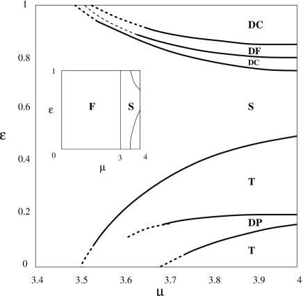
Figure 1: Phase space diagram showing different features of coupled dynamics in the two parameter space of $\mu$ and $\epsilon$ for three nodes bipartite network with logistic map as local map and coupling function $g(x)=f(x)$. Different regions are T. Turbulent region, DP. Driven periodic, DF. Driven fixed point, DC. Driven Chaotic, S. Self organized region and F. Fixed point. Region boundaries are determined based on the asymptotic behaviour using several initial conditions, synchronization behaviour and the largest Lyapunov exponent. The dashed lines indicate uncertainties in determining the boundaries. The inset shows the phase diagram for the entire range of parameter $\mu$ from 0 to 4.

Case I. Synchronization to Fixed point: Nodes get synchronized to a fixed point with one set of nodes having one value and the other set of nodes having a different value such as $(x^{1}_{t}=x^{2}_{t}=X^{\star}_{1})$ and ($x^{3}_{t}=X^{\star}_{2}$). Eigenvalues of Jacobian matrix (45) with $g(x)=f(x)$ are,

$$\Lambda_{1} = (1-\epsilon)f^{\prime}_{1}$$ (49a)

$$\Lambda_{2,3} = \frac{1-\epsilon}{2}(f^{\prime}_{1}+f^{\prime}_{2})$$ (49b)

$$\pm\frac{1}{2}\sqrt{(1-\epsilon)^{2}(f^{\prime}_{1}+f^{\prime}_{2})^{2}-4(1-2\epsilon)f^{\prime}_{1}f^{\prime}_{2}}$$

where $f^{\prime}_{1}$ and $f^{\prime}_{2}$ are the derivatives at $X_{1}$ and $X_{2}$ respectively. By putting the condition that the magnitude of the above eigenvalues should be less than one, we get the $\epsilon$ range for which the fixed point state is stable. When the first two nodes synchronize with each other, the three coupled maps system behaves like just two coupled maps and within this $\epsilon$ range all the solutions are those of the two coupled maps. The expressions for $X^{\star}_{1}$ and $X^{\star}_{2}$ are

$$X^{\star}_{1,2}=\frac{(1-\mu+2\mu\epsilon)\pm\sqrt{(1-\mu+2\mu\epsilon)^{2}-4\epsilon(1-\mu+2\mu\epsilon)}}{2\mu(2\epsilon-1)}$$ (50)

From Eqs. (49a) and (49b) the coupling strength values for which the fixed point solution is stable must satisfy

$$|(1-\epsilon)f^{\prime}_{1}|<1$$

and the following condition

$$\frac{1}{2}\left(1+\sqrt{\frac{3}{\mu(\mu-2)}}\right)<\epsilon<\frac{3+2\mu(\mu-2)+\sqrt{(3+2\mu(\mu-2))^{2}-4\mu(\mu-2)(\mu-1)^{2}}}{4\mu(\mu-2)};.$$ (51)

Case II. Synchronization to period two orbit: Consider a periodic orbit of period two where the first two nodes are d-synchronized and have the value $X_{1}^{p}$, and the third node has has the value $X_{2}^{p}$. The period two orbit is obtained by interchanging these two values at successive time steps. The Jacobian matrix for this periodic orbit can be written as $J=J_{1}J_{2}$ where

$$J_{1}=\left(\begin{array}[]{cccc}(1-\epsilon)f^{\prime}_{1}&0&\epsilon f^{\prime}_{2}\\ 0&(1-\epsilon)f^{\prime}_{1}&\epsilon f^{\prime}_{2}\\ \frac{\epsilon}{2}f^{\prime}_{1}&\frac{\epsilon}{2}f^{\prime}_{1}&(1-\epsilon)f^{\prime}_{2}\end{array}\right)$$ (52)

where $f_{1}^{\prime}$ and $f_{2}^{\prime}$ are derivatives at $X_{1}^{p}$ and $X_{2}^{p}$ respectively and $J_{2}$ is obtained by interchanging suffixes 1 and 2 in the expression for $J_{1}$. Eigenvalues of $J$ are given by

$$\Lambda_{1} = (1-\epsilon)^{2}f^{\prime}_{1}f^{\prime}_{2}$$ (53a)

$$\Lambda_{2,3} = \left(\frac{\epsilon}{2}(f^{\prime}_{1}+f^{\prime}_{2})\pm\sqrt{\frac{\epsilon^{2}}{4}(f^{\prime}_{1}+f^{\prime}_{2})^{2}+(1-2\epsilon)f^{\prime}_{1}f^{\prime}_{2}}\right)^{2}$$ (53b)

For $f(x)$ given by logistic map, the periodic points are

$$X^{p}_{1,2}=s\pm\sqrt{s(1-s-\frac{1}{\mu})},$$ (54)

where

$$s=\frac{1}{2}\left(1+\frac{1}{\mu(1-2\epsilon)}\right).$$

After imposing the condition $\left|\Lambda_{1,2,3}\right|<1$ we can get the $\epsilon$ range for which the period two orbit is stable. The first eigenvalue gives us the condition that

$$1-\epsilon<\frac{|1-2\epsilon|}{\sqrt{(1+\mu-2\epsilon\mu)(4\epsilon-1+\mu-2\epsilon\mu)}}.$$ (55)

The other two eigenvalues give us the same condition as in Eq. (51) except that $\epsilon$ in this inequality is substituted by $1-\epsilon$ similar to the case of two coupled maps driven-T1S2 . For logistic map with $\mu=4$, this range is given by $0.16..<\epsilon<0.20..$.

Case III. Synchronization of all three nodes: It is also possible that all the three nodes get synchronized (s-synchronization). The eigenvalues of Jacobian matrix for this synchronized state ($x^{1}_{t}=x^{2}_{t}=x^{3}_{t}=x_{t}$) can simply be written from Eqs. (49a) and (49b), by putting $f^{\prime}_{1}=f^{\prime}_{2}=f^{\prime}(x_{t})$, which gives Lyapunov exponents as,

$$\lambda_{1} = \lambda_{u}=\frac{1}{\tau}\lim_{\tau to\infty}\sum_{t=1}^{\tau}\ln|f^{\prime}(x_{t})|$$ (56a)

$$\lambda_{2} = \ln(1-\epsilon)+\lambda_{u}$$ (56b)

$$\lambda_{3} = \ln(1-2\epsilon)+\lambda_{u}$$ (56c)

where $\lambda_{u}$ is the Lyapunov exponent for an uncoupled map $f(x)$. For synchronous orbits to be stable, the two Lyapunov exponents ($\lambda_{2}$ and $\lambda_{3}$) corresponding to the transverse eigenvectors should be negative. We get the following $\epsilon$ range for which both the transverse eigenvalues are negative,

$$1-e^{-\lambda_{u}}<\epsilon<\frac{1}{2}(1+e^{-\lambda_{u}})$$ (57)

In this region coupled dynamics may lie on a chaotic or a periodic attractor depending upon the value of $\lambda_{u}$. For $f(x)=\mu x(1-x)$ with $\mu=4$, $\lambda_{u}=\ln 2$ and thus the range of stability of the s-synchronization of all three nodes is (0.5, 0.75) and the dynamics is chaotic.

Figure 2: The figure shows the variation of two sets of difference, $|x^{1}_{t}-x^{2}_{t}|$ (open circles) and $|x^{1}_{t}-x^{3}_{t}|$ (crosses) for a three nodes network as a function of the coupling strength $\epsilon$ for $f(x)=\mu x(1-x)$ with $\mu=4$ and $g(x)=f(x)$. For each $\epsilon$, 100 values of the differences are plotted after an initial transient.

Phase diagram in $\mu-\epsilon$ plane: Fig. 1 shows different phases in the $\mu-\epsilon$ plane for three nodes bipartite network with $g(x)=f(x)$. For $\mu<3$ we get a fixed point solution. To understand the remaining phase diagram consider the line $\mu=4$. Fig. 2 shows two sets of differences between the values of variables, $|x^{1}-x^{2}|$ (open circles) and $|x^{1}-x^{3}|$ (crosses) as a function of the coupling strength $\epsilon$. Bipartite d-synchronized state and global s-synchronized state are clearly seen. Fig. 3(a) shows largest Lyapunov exponent and Fig. 4(a) shows the fractions of inter- and intra- couplings, $f_{inter}$ and $f_{intra}$, as a function of $\epsilon$ for $mu=4$. The two quantities $f_{\rm intra}$ and $f_{\rm inter}$ act as measures for the intra-cluster couplings and the inter-cluster couplings and are defined as sarika-REA1 ; sarika-REA2 ,

$$f_{\rm intra} = \frac{N_{\rm intra}}{N_{c}}$$ (58a)

$$f_{\rm inter} = \frac{N_{\rm inter}}{N_{c}}$$ (58b)

where $N_{\rm intra}$ and $N_{\rm inter}$ are the numbers of intra- and inter-cluster couplings respectively. In $N_{\rm inter}$, couplings between two isolated nodes are not included. Initially for small coupling strength values nodes are in turbulent region with no cluster formation at all (region T). As the coupling strength increases beyond a critical $\epsilon_{c}$ we get bipartite d-synchronized state (region DP). This region corresponds to the Case II of period two orbits discussed above in this subsection. When the coupling strength increases further we get a reappearance of turbulent region. As the coupling strength is increased further all the nodes are synchronized giving one cluster with global s-synchronization (region S). This region corresponds to the case III discussed above and the range of $\epsilon$ for this region is given by Eq. (57). In this region the coupled dynamics lies on a chaotic attractor. In the last three regions (DC, DP and DC), we get driven bipartite synchronization. The middle region (DP) displays driven fixed point solution (case I) while the other regions show chaotic behaviour.

For $\mu<4$, the coupling strength range where all the nodes are synchronized (region S) increases in size and the coupling strength ranges where nodes show d-synchronization shift towards the nearest boundaries $\epsilon=0$ and $\epsilon=1$.

Figure 3: (a) The figure shows the largest Lyapunov exponent $\lambda$ as a function of the coupling strength $\epsilon$ for the three nodes bipartite network with logistic map as local map with $\mu=4$ and $g(x)=f(x)$. (b) Same as for (a) but for a bipartite network of 50 nodes with $N1=N2=25$.

Figure 4: (a) The figure shows the fractions of inter- and intra-cluster couplings, $f_{inter}$ and $f_{intra}$, as a function of the coupling strength $\epsilon$ for the three nodes bipartite network, logistic map as local map with $\mu=4$ and $g(x)=f(x)$. The values are obtained by averaging over 50 random initial conditions. (b) Same as for (a) but for a bipartite network of 50 nodes with $N1=N2=25$.

Coupling function $g(x)=x$: Numerical analysis shows periodic solutions which we now consider in detail. When the first two nodes are d-synchronized the solutions of the dynamical equations are similar to the two nodes case. This simplifies the analysis considerably.

Case I. Driven synchronization to period two orbit: First we consider the case where the coupled dynamics shows periodic attractor with period two behaviour and the variables take the values

$$x^{1}_{t}=x^{2}_{t}=x^{3}_{t+1} = X_{1}^{p}$$

$$x^{3}_{t}=x^{1}_{t+1}=x^{2}_{t+1} = X^{p}_{2}$$ (59)

Using the product of Jacobians of Eq. (45) for two consecutive time steps the eigenvalues for this periodic orbit can be easily obtained. The eigenvalue $\Lambda_{d}$ associated with the difference variable $d_{t}$ is given by

$$\Lambda_{d}=(1-\epsilon)^{2}f_{1}^{\prime}f^{\prime}_{2},$$ (60)

The other two eigenvalues are the eigenvalues of product matrix $J_{1}J_{2}$, where $J_{1}$ is given by Eq. (15) and hence the eigenvalues are given by Eq. (16). The solution of the periodic orbit is the same as for two coupled maps (Eq. (18)). Using all the three eigenvalues of Jacobian matrix, the coupling strength range, for which the periodic orbit given by Eq. (59) is stable, is given by

$$\max\left(1-\frac{1}{\sqrt{f^{\prime}_{1}f^{\prime}_{2}}},\frac{|f_{1}^{\prime}f_{2}^{\prime}|-1}{|f_{1}^{\prime}f_{2}^{\prime}|+1}\right)<\epsilon<1$$ (61)

The periodic points $X_{1}$ and $X_{2}$ are also the periodic points of uncoupled map $f$ (Eq. (13)). For logistic map, we get the following range of coupling strength in terms of logistic map parameter $\mu$,

$$1-\frac{2}{\mu^{2}-2\mu-3}<\epsilon<1$$ (62)

which is the same as Eq. (19). The lower bound of $\epsilon$ matches exactly with the boundary between the regions IV-DP and IV-DQ of Fig. 1 of Ref. sarika-REA2 and regions DP and DQ of Fig. 5.

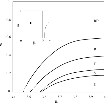
Figure 5: Phase space diagram showing different features of coupled dynamics in the two parameter space of $\mu$ and $\epsilon$ for three nodes bipartite network with logistic map as local map and coupling function $g(x)=x$. Different regions are T. Turbulent region, DP. Driven periodic, DF. Driven fixed point, DQ. Driven Quasiperiodic, DC. Driven Chaotic, S. Self organized region and F. Fixed point. Region boundaries are determined based on the asymptotic behaviour using several initial conditions, synchronization behaviour and the largest Lyapunov exponent. The dashed lines indicate uncertainties in determining the boundaries. The inset shows the phase diagram for the entire range of parameter $\mu$ from 0 to 4.

Figure 6: The figure shows the variation of two sets of difference, $|x^{1}_{t}-x^{2}_{t}|$ (open circles) and $|x^{1}_{t}-x^{3}_{t}|$ (crosses) for a three nodes network as a function of the coupling strength $\epsilon$ for $f(x)=\mu x(1-x)$ with $\mu=4$ and $g(x)=x$. For each $\epsilon$, 100 values of the differences are plotted after an initial transient.

Case II. Synchronization of all three nodes: All three nodes get synchronized for a small coupling strength region with dynamics lying on periodic orbits of period two such that

$$x^{1}_{t}=x^{2}_{t}=x^{3}_{t}=X^{p}_{1}$$

$$x^{1}_{t+1}=x^{2}_{t+1}=x^{3}_{t+1}=X^{p}_{2}$$ (63)

The eigenvalue of the Jacobian for this periodic orbit for the difference variable is simply $(1-\epsilon)^{2}f^{\prime}_{1}f^{\prime}_{2}$ and the other two eigenvalues are the same as for two coupled maps and are given by Eq. (12). The periodic points are given by Eq. (14). The coupling strength range for which all three nodes are synchronized for logistic map with $\mu=4$, is $0.18...<\epsilon<0.24...$ which is same as Case I for two coupled maps with $g(x)=x$.

Phase diagram in $\mu-\epsilon$ space: Fig. 5 shows different phases in the $\mu-\epsilon$ plane for three nodes bipartite network with $g(x)=x$. For $\mu<3$ we get a fixed point solution. To understand the remaining phase diagram consider the line $\mu=4$. Fig. 6 shows two sets of differences between the values of variables, $|x^{1}-x^{2}|$ (open circles) and $|x^{1}-x^{3}|$ (crosses) as a function of the coupling strength $\epsilon$. Bipartite d-synchronized state and global s-synchronized state are clearly seen. Fig. 7(a) shows largest Lyapunov exponent and Fig. 8(a) shows the fractions of inter- and intra- couplings, $f_{inter}$ and $f_{intra}$, as a function of $\epsilon$ for $mu=4$. Initially for small coupling strength values nodes are in turbulent region with no cluster formation at all (region T). As the coupling strength increases beyond a critical $\epsilon_{c}$, we get global s-state (region S). This region is the case II considered above. When the coupling strength increases further we get a reappearance of turbulent region. In the last two regions we get driven bipartite synchronization (regions DQ and DP). The last region corresponds to case I of period two discussed above in this subsection and the critical coupling strength for it is given by Eq. (61).

For $\mu<4$, the coupling strength region for d-synchronization gets wider and that for s-synchronization gets thiner with a shift towards $\epsilon=0$.

IV.2 Complete bipartite networks

Let us now consider a complete bipartite network of $N=N1+N2$ nodes and dynamics defined by Eq. (39). We define a bipartite synchronized state of the bipartite network as the one that has that all $N1$ elements of the first set synchronized to some value, say $X_{1}(t)$, and all $N2$ elements of the second set synchronized to some other value, say $X_{2}(t)$. Linear stability analysis of the bipartite synchronized state can be done using the Jacobian matrix,

$$J_{t}=\left(\begin{array}[]{cccccccc}(1-\epsilon)f^{\prime}_{1}&0&\dots&0&\frac{\epsilon}{N2}g^{\prime}_{2}&\frac{\epsilon}{N2}g^{\prime}_{2}&\dots&\frac{\epsilon}{N2}g^{\prime}_{2}\\ \vdots&\vdots&\vdots&\vdots&\vdots&\vdots&\vdots&\vdots\\ 0&0&\dots&(1-\epsilon)f^{\prime}_{1}&\frac{\epsilon}{N2}g^{\prime}_{2}&\frac{\epsilon}{N2}g^{\prime}_{2}&\dots&\frac{\epsilon}{N2}g^{\prime}_{2}\\ \frac{\epsilon}{N1}g^{\prime}_{1}&\frac{\epsilon}{N1}g^{\prime}_{1}&\dots&\frac{\epsilon}{N1}g^{\prime}_{1}&(1-\epsilon)f^{\prime}_{2}&0&\dots&0\\ \vdots&\vdots&\vdots&\vdots&\vdots&\vdots&\vdots&\vdots\\ \frac{\epsilon}{N1}g^{\prime}_{1}&\frac{\epsilon}{N1}g^{\prime}_{1}&\dots&\frac{\epsilon}{N1}g^{\prime}_{1}&0&0&\dots&(1-\epsilon)f^{\prime}_{2}\\ \end{array}\right)$$ (64)

where $g^{\prime}_{1}$ and $g^{\prime}_{2}$ are the derivative of $g(x)$ at $X_{1}$ and $X_{2}$ respectively. It is easy to see that the eigenvectors and eigenvalues of the above Jacobian matrix can be divided into three sets, $A,B,C$, as,

set	Eigenvectors		Eigenvalue		No of eigenvalues		condition
$A$	$(\alpha_{1}\dots\alpha_{N1},0\cdots 0)$		$(1-\epsilon)f_{1}^{\prime}$		$N1-1$		$\Sigma{\alpha}=0$
$B$	$(0\dots 0,\beta_{1}\dots\beta_{N2})$		$(1-\epsilon)f_{2}^{\prime}$		$N2-1$		$\Sigma{\beta}=0$
$C$	$(\alpha,\dots\alpha,\beta,\dots\beta)$		-		2		-

Here, ($\alpha_{1},\ldots\alpha_{N1}$), ($\beta_{1},\ldots\beta_{N2})$ and $\alpha,\beta$ are complex numbers satisfying the conditions specified in the last column. The two eigenvalues corresponding to the set $C$ are the eigenvalues of the matrix

$$\left(\begin{array}[]{ccc}(1-\epsilon)f_{1}^{\prime}&\epsilon g_{2}^{\prime}\\ \epsilon g_{1}^{\prime}&(1-\epsilon)f_{2}^{\prime}\end{array}\right)$$ (65)

We make the following observations. (a) The three sets of eigenvectors, $A,B,C$, are orthogonal to each other and the total space of eigenvectors may be written as a direct sum of these three sets. (b) The three sets of eigenvectors do not mix with each other under time evolution. (c) The eigenvectors belonging to the first two sets ($A$ and $B$) are also the eigenvectors of the product of any number of Jacobian matrices under time evolution. (d) The two sets of eigenvectors $A$ and $B$ are transverse to the synchronization manifold which is defined by the last set of eigenvectors $C$.

Lyapunov exponents corresponding to the transverse eigenvectors can be easily written as

$$\lambda_{i} = \ln|(1-\epsilon)|+\frac{1}{\tau}\lim_{\tau\to\infty}\sum^{\tau}_{t=1}\ln|f^{\prime}(X_{1})|,$$ (66a)

$$\,\,\,\,\,{\rm for}\,i=1,\ldots,N1-1$$

$$\lambda_{i} = \ln|(1-\epsilon)|+\frac{1}{\tau}\lim_{\tau\to\infty}\sum^{\tau}_{t=1}\ln|f^{\prime}(X_{2})|,$$ (66b)

$$\,\,\,\,\,{\rm for}\,i=N1,\ldots,N-2.$$

The synchronized state is stable provided the transverse Lyapunov exponents are negative. If $f^{\prime}$ is bounded as is the case for the logistic map then from Eqs. (66) we see that for $\epsilon$ larger than some critical value, $\epsilon_{c}(<1)$, bipartite synchronized state will be stable. Note that this bipartite synchronized state will be stable even if one or both the remaining Lyapunov exponents corresponding to the set $C$ are positive, i.e. the trajectories are chaotic.

Now we study the periodic behaviour of coupled dynamics of Eq. (39). Here we consider two cases, fixed point attractor and periodic attractor with period two, as we studied for three nodes.

Figure 7: (a) The figure shows the largest Lyapunov exponent $\lambda$ as a function of the coupling strength $\epsilon$ for the three nodes bipartite network with logistic map as local map with $\mu=4$ and $g(x)=x$. (b) Same as for (a) but for a bipartite network of 50 nodes with $N1=N2=25$.

IV.2.1 Coupling function $g(x)=f(x)$

The fixed point bipartite synchronized solution with one set of nodes taking value $X_{1}^{*}$ and the other set $X_{2}^{*}$, is given by Eq. (50). Jacobian matrix for this solution gives three sets of eigenvalues, first set of $N1-1$ degenerate eigenvalues $(1-\epsilon)f^{\prime}_{1}$, second set of $N2-1$ degenerate eigenvalues $(1-\epsilon)f^{\prime}_{2}$ and third set of two eigenvalues given by Eq. (49b). The conditions for the stability of this solution is given by Eq. (51) and $|(1-\epsilon)f^{\prime}_{1},2|<1$.

The bipartite synchronous period two solution is obtained when one set of nodes take the value $X^{p}_{1}$ and the other set of nodes take the value $X^{p}_{2}$ and the two values alternate in time. This solution is the same as given by Eq. (54). The eigenvalues (Eqs. (53a) and (53b), with the $N-2$ fold degeneracy of $\Lambda_{1}$) and the conditions for stability of the solution are the same as for Case II of three nodes with $g(x)=f(x)$.

The global synchronized solution where all nodes of the bipartite network are synchronized, has the same Lyapunov exponents (except the degeneracy) as in Eqs. (56c) and the stability criterion is again given by Eq. (57).

IV.2.2 Coupling function $g(x)=x$

Consider a periodic orbit of period two with bipartite synchronized state where all nodes of one set take value $X_{1}$ and and the other set $X_{2}$ and two values alternate in time. The solutions is same as for case I of three nodes bipartite network. The stability ranges are given by Eqs. (61) and (62).

Figure 8: (a) The figure shows the fractions of inter- and intra-cluster couplings, $f_{inter}$ and $f_{intra}$, as a function of the coupling strength $\epsilon$ for the three nodes bipartite network, logistic map as local map with $\mu=4$ and $g(x)=x$. The values are obtained by averaging over 50 random initial conditions. (b) Same as for (a) but for a bipartite network of 50 nodes with $N1=N2=25$.

IV.3 Lyapunov Function Analysis

For the complete bipartite networks, Lyapunov function as defined by Eq. (4), for any two nodes belonging to the same set is given by

$$V^{ij}_{t+1}=[(1-\epsilon)(f(x^{i}_{t})-f(x^{j}_{t}))]^{2}$$ (67)

Expanding around $x^{j}_{t}$ gives the ratio of Lyapunov functions at two successive times,

$$\frac{V^{ij}_{t+1}}{V^{ij}_{t}}=(1-\epsilon)^{2}\left[f^{\prime}(x^{j}_{t})+\frac{x^{i}_{t}-x^{j}_{t}}{2}f^{\prime\prime}(x^{j}_{t})+{\cal O}((x^{i}_{t}-x^{j}_{t})^{2})\right]^{2}$$

If the term in the square bracket on the RHS is bounded then there will be a critical value of $\epsilon$ beyond which $\frac{V^{ij}_{t+1}}{V^{ij}_{t}}<1$ and thus the bipartite synchronized state will be stable.

We see that for d-synchronization, Lyapunov function for any pair of nodes does not depend on the size of the complete bipartite network and type of the coupling because in the expression for Lyapunov function, contribution of such couplings cancel out. This is not the case for globally coupled networks where contribution of the coupling terms for the two nodes under consideration do not exactly cancel and the size of the network has an effect on the asymptotic behaviour.

For the logistic map and using $0\leq x^{i}_{t}+x^{j}_{t}\leq 2$ and Eq. (5), we get the following range for $\epsilon$ values for synchronization of nodes $i$ and $j$,

$$\frac{\mu-1}{\mu}\leq\epsilon\leq 1$$ (68)

A better $\epsilon$ range can be obtained by taking a more appropriate boundary as $X^{-}<x^{i}_{t}+x^{j}_{t}<X^{+}$, which gives

$$1-\frac{1}{\mu A}<\epsilon\leq 1$$

where $A$ is defined after Eq. (36).

IV.4 Journey from small network to large network

To understand the features of d-synchronization in bipartite network and comparison of this large network with the network of three nodes, here we briefly present the numerical results for logistic map with $\mu=4$. Fig. 3(b) plots the largest Lyapunov exponent as function of $\epsilon$ and Fig. 4(b) plots $f_{inter}$ and $f_{intra}$ as a function of $\epsilon$ for a bipartite network with $g(x)=f(x)$ and $\mu=4$. Comparing with the three nodes network (Figs. 3(a) and 4(a)) we find that the major difference is in the range $0.20..<\epsilon<0.5$ where the turbulent region reappears for the three nodes network while the mixed region having both d- and s-clusters is observed for the larger bipartite networks. The region boundaries for the period two, globally s-state and fixed point are the same for the three nodes and larger bipartite networks and are the same as given for cases II, III and I respectively for three nodes bipartite network with $g(x)=f(x)$. We see that most of the dynamical features and synchronized cluster formation in coupled map bipartite networks with three nodes get carried over to the larger bipartite networks.

As in the case $g(x)=f(x)$ there is a similarity between the three nodes bipartite network and the larger bipartite networks for $g(x)=x$. Fig. 7(b) plots the largest Lyapunov exponent as a function of $\epsilon$ and Fig. 8(b) plots $f_{inter}$ and $f_{intra}$ as a function of $\epsilon$ for a bipartite network with $g(x)=x$ and $\mu=4$. Comparing with the three nodes network (Figs. 7(a) and 8(a)) we find that the main difference is in the range $0.24..<\epsilon<0.35..$ where the turbulent region reappears for the three nodes network while d-synchronization appears for the larger bipartite networks. The other regions show a very similar behaviour for both three nodes and larger bipartite networks.

IV.5 S- and D-synchronization

The analysis presented so far shades some light on the dynamical origin of the two types of synchronization namely self-organized and driven, that we have studied. In s-synchronization the clusters have dominant intra-cluster couplings while in d-synchronization they have dominant inter-cluster couplings. We consider two nodes and globally coupled networks as simple examples of s-synchronization while three nodes and complete bipartite networks as simple examples of d-synchronization. The dynamics of the difference variable and Lyapunov function analysis are useful for understanding the difference between the two mechanisms of cluster formation.

From Eq. (8a)(b) we see that in the dynamics of the difference variable $d_{t}$ for the two nodes network the coupling term adds an extra decay term. This is also seen from the expression (21) for Lyapunov function. On the other hand, from Eq. (44b) we see that in the dynamics of the difference variable for the three nodes network the coupling terms with the third variable cancel out (see also Eq. (67) for Lyapunov function). The situation is more complicated when we consider larger networks. The d-synchronization shows the same trend i.e. cancellation of the coupling terms in the dynamics of the difference variables and as well as in the expression for Lyapunov function (Eq. (67)). On the other hand, Eq. (34) for Lyapunov function for the globally coupled maps shows that the direct coupling term between the two nodes under consideration adds an extra term in the difference variable while the coupling terms to other variables cancel out.

The analysis presented in this paper is for exact synchronization while Ref. sarika-REA2 considers phase synchronized clusters. However, we feel that the dynamical origin for the two mechanisms of cluster formation should be similar in both cases. This is supported by the very similar features of plots of phase space, largest Lyapunov exponent, $f_{inter}$ and $f_{intra}$ for the three nodes and complete bipartite networks and the corresponding plots for several networks considered in Ref. sarika-REA2 .

V Conclusion

We have studied s- and d-synchronization in coupled map networks using some simple networks, namely two and three node networks and their natural generalization to globally coupled and bipartite networks respectively. For this study we use both linear stability analysis and Lyapunov function approach. We see that for the difference variable for any two nodes that are in d-synchronization all the coupling terms cancel out whereas when they are in s-synchronization though coupling terms for couplings to other nodes may cancel, the coupling terms corresponding to the direct coupling between the two nodes under consideration do not cancel.

The phase diagrams for three nodes network has features very similar to the different kinds of networks studied in Ref. sarika-REA2 . (The phase diagrams for two nodes, not shown in this paper, have similar features except the d-synchronization which needs at least three nodes to manifest itself.) Under the time evolution, the coupled dynamics lies on different periodic or chaotic attractors with varying coupling strength values. The type of coupling function plays an important role in the time evolution of the coupled dynamics. We also see that most of the features of coupled dynamics of small networks with two or three nodes, are carried over to the larger networks of the same type.

This work was supported in part by the National Science Council of the Republic of China (Taiwan) under Grant No. NSC 91-2112-M-001-056.

References

- (1) S. H. Strogatz, Nature, 410, 268 (2001) and references theirin.
- (2) R. Albert and A. L. Barabäsi, Rev. Mod. Phys. 74, 47 (2002) and references theirin.
- (3) D. J. Watts and S. H. Strogatz, Nature (London) 393, 440 (1998).
- (4) A. -L. Barabäsi, R. Albert, Science, 286, 509 (1999).
- (5) C. Koch and G. Laurent, Science 284, 96 (1999).
- (6) S. Wasserman and K. Faust, Social Network Analysis, Cambridge Univ. Press, Cambridge 1994.
- (7) R. Albert, H. Jeong, A. -L. Barabäsi, Nature 401, 130 (1999); R. Albert, H. Jeong, A. -L. Barabäsi, Nature 406, 378 (2000).
- (8) H. Jeong, B. Tomber, R. Albert, Z. N. Oltvai, A. -L. Barabäsi, Nature, 407, 651 (2000).
- (9) Richard J. Williams, Nea D. Martinez, Nature, 404, 180 (2000).
- (10) S. Render, Euro. Phys. J. B. 4, 131 (1998); M. E. J. Newman, Phys. Rev. E 64 016131 (2001).
- (11) S. Jalan and R. E. Amritkar, Phys. Rev. Lett. 90, 0141011 (2003); R. E. Amritkar and S. Jalan, Physica A 321, 220 (2003).
- (12) S. Jalan and R. E. Amritkar, arXiv:nlin.CD/0307029 and references therein.
- (13) K. Kaneko, Phys. Rev. Lett. 65, 1391 (1990); Physica D, 41, 137 ( 1990 ); Physica D 124, 322 (1998).
- (14) Y. L. Maistrenko, V. L. Maistrenko, O. Popovych and E. Mosekilde, Phys. Rev. E 60 2817 (1999).
- (15) Y. Kuramoto, Chemical Oscillations, Waves, and Turbulence (Springer-Verlag, Berlin, 1984).
- (16) A. Pikovsky, M. Rosenblum and J. Kurth, Synchronization : A Universal Concept in Nonlinear Dynamics (Cambridge University Press, 2001).
- (17) H. Fujisaka and T. Yamada, Prog. Theo. Phys. 69, 32 (1983); ibid 74, 918 (1985).
- (18) R. E. Amritkar, P. M. Gade and A. D. Gangal, Phys. Rev. A 44, R3407 (1991).
- (19) P. M. Gade, Phys. Rev. E, 54 64 (1996).
- (20) M. Ding and W. Yang, Phys Rev E, 56 4009, (1997).
- (21) M. Soins and S. Zhou, Physica D 165, 12 (2002).
- (22) J. Jost and M. P. Joy, Phys. Rev. E 65, 016201 (2002).
- (23) S. Wiggins, Introduction to Applied Nonlinear Dynamical Systems and Chaos (Springer-Verlag, 1990).
- (24) R. He and P. G. Vaidya, Phys. Rev. A, 46 7387 (1992); Phys. Rev. E 57 1532 (1998).
- (25) Q. Zhilin and G. Hu, Phys. Rev. E, 49, 1099 (1994).
- (26) In this case the increased range of stability with increasing is accompanied by a decrease in the basin of attraction. Hence, numerically starting from random initial conditions this incremental part of the range is not observed.