Fluctuation formula in the Nosé-Hoover thermostated Lorentz gas

Abstract

In this paper we examine numerically the Gallavotti-Cohen fluctuation formula for phase-space contraction rate and entropy production rate fluctuations in the Nosé-Hoover thermostated periodic Lorentz gas. Our results indicate that while the phase-space contraction rate fluctuations violate the fluctuation formula near equilibrium states, the entropy production rate fluctuations obey this formula near and far from equilibrium states as well.

I Introduction

In recent years a large number of papers focused on various fluctuation formulas (FFs) with both theoretical and numerical tools, and today these seem to be one of the most interesting results in the field of statistical physics of nonequilibrium systems ftreview . This behavior was observed numerically in a system of thermostated fluid particles undergoing shear flow shearflow . It was an important property of the FF that it seemed to be valid for large external forcings as well chaodyn , therefore it was considered that it could shed some light on the thermodynamical behavior of systems far from equilibrium. Consequently, significant theoretical efforts have been made to find a common property behind the observed FF and these efforts resulted in various fluctuation theorems (FTs): the Gallavotti-Cohen approach built on the chaotic hypothesis gcft ; dynens , the Evans-Searles theorems es , deterministic local FT revdamp , the FT for stochastic systems kurchan ; es4 ; lebspo , the theorem of Maes established on the Gibbs Property maes , and the FT for open systems tel . The Gallavotti-Cohen FT/FF serves as the basis of the numerical investigations presented in this paper.

All of the applied theoretical methods shared the property of putting extra presumptions on the physical systems (i.e., chaoticity, stochasticity) that could not be proved a priori. This situation naturally raised the need to study the FF numerically and compare the numerical results to the theoretical predictions. Up to now several physical models have been investigated numerically, such as the two-dimensional (2D) reversibly damped fluids revdamp , the chains of weakly interacting cat maps catmap , the Fermi-Ulam-Pasta chain anhlatt , and the periodic Lorentz Gas (PLG) thermostated by the Gaussian isokinetic (GIK) thermostat exptest ; flform .

The FF is a symmetry property of the probability density function (PDF) of a dynamically measured quantity $\pi$ connecting the probabilities of measuring $\pi$ values with equal magnitudes but opposite signs. More precisely, let $\pi_{\tau}(t)$ denote the quantity $p$ averaged over a time interval of length $\tau$ centered around time $t$: $\pi_{\tau}(t)=\frac{1}{\tau}\int\limits_{-{\tau}/{2}}^{{\tau}/{2}}p(t+t^{\prime})\,\mathrm{d}t^{\prime}$. Considering it as a stochastic variable $x$, its statistical properties in a steady state can be characterized by the PDF $\Pi_{\tau}(x)$. The FF states that the PDF $\Pi_{\tau}(x)$ has the following property:

$$\lim_{\tau\to\infty}\frac{1}{\tau}\ln\frac{\Pi_{\tau}(x)}{\Pi_{\tau}(-x)}=x\,.$$ (1)

In other words, for large enough $\tau$ values the probability of observing $-\pi_{\tau}$ is exponentially smaller than the probability of observing $\pi_{\tau}$ .

In exptest ; flform the examined physical quantity $\pi_{\tau}(t)$ was the phase-space contraction rate (PSCR), which due to this special property of the applied GIK thermostat was equal to the thermodynamical entropy production rate (EPR) at any given time. However, this identity does not hold in general epr , and PSCR and EPR fluctuations can have different PDFs as, e.g., in the case of Nosé-Hoover thermostated systems (see Sec. II). The theoretical methods using the Sinai-Ruelle-Bowen (SRB) measure gcft ; shearflow to calculate the probabilities of trajectory segments predict that the quantity obeying the FF is the PSCR and further nontrivial theoretical efforts are needed to establish similar results for the EPR fluctuations epr .

The main purpose of examining the Nosé-Hoover (NH) thermostated PLG is to investigate which of the above-mentioned physical quantities obey the FF in a system, where the corresponding PDFs are not identical. In addition to this, checking the NH thermostated PLG numerically against the FF is in itself an important task, given that the NH thermostat is one of the two generally used dynamical thermostats; the transport properties of this model have been recently investigated in nosehoover . In Sec. II we describe the examined model; in Sec. III we present our numerical results; and in Sec. IV we summarize our conclusions.

II The System

One of the most investigated models suitable for studying transport phenomena is the field-driven thermostated periodic Lorentz Gas. This model consists of a charged particle subjected to external electric field and moving in the lattice of elastic scatterers. Due to the applied electric field, one must use a thermostating mechanism to achieve a steady state in the system; such a tool is a dynamical thermostat. Two types of dynamical thermostats have been applied to the PLG up to now: the GIK thermostat producing microcanonical distribution gik and the Nosé-Hoover thermostat producing canonical distribution in equilibrium nosehoover ; thermostats .

We present the equations of motion of the two-dimensional NH thermostated PLG in dimensionless form: mass and electric charge are measured in units of the particle’s mass $m$ and charge $q$ and the unit length is chosen to be the radius of the scatterers ($R=1$). Let ${\bf q}=\left(q_{1},q_{2}\right)$ denote the position and ${\bf p}=\left(p_{1},p_{2}\right)$ the momentum of the particle, then the phase-space vector of the system is ${\mathbf{\Gamma}}=\left({\bf q},{\bf p},\zeta\right)$, where $\zeta$ is the state variable of the thermal reservoir. Between two subsequent collisions the state of the system is evolved smoothly by the differential equation

$$\dot{\bf q} = {\bf p}\,,$$

$$\dot{\bf p} = {\bf E}-\zeta{\bf p}\,,$$ (2)

$$\dot{\zeta} = \frac{1}{\tau^{2}_{resp}}\left(\frac{p^{2}}{2T}-1\right)\,,\$$

and is transformed abruptly at every elastic collision. In this equation ${\bf E}$ is the the external electric field, $\tau_{resp}$ is the response time of the reservoir, and $T$ is the temperature satisfying $\left<p^{2}\right>=2T$.

In the simulations presented in this paper we have used a square lattice of circular scatterers, however, we have investigated numerically other lattices as well (e.g, triangular), but have not found any relevant differences concerning the results presented in Sec. III.

Energy dissipation can be measured by the phase-space contraction rate $\sigma$ and can be computed by taking the divergence of the right-hand side of Eq. (II) as:

$$\sigma(t)=-\mbox{div}\,{\bf\dot{\Gamma}}(t)=\zeta(t)\,.$$ (3)

The entropy production rate $\xi$ can be formally defined by the expression of irreversible thermodynamics

$$\xi(t)=\frac{{\bf J}(t){\bf E}}{T}=\frac{{\bf p}(t){\bf E}}{T}\,,$$ (4)

where $T$ is the kinetic temperature. We note that this quantity is identical to the dissipation function of the Evans-Searles theorem ftreview . It can be shown that in this model $\left<\sigma\right>=\left<\xi\right>$, however, the identity $\sigma(t)=\xi(t)$ does not hold at all times, as opposed to the case of the GIK thermostated PLG.

III Numerical Results

The objective of the numerical simulation is to measure the PDFs $\Sigma_{\tau}(x)$ and $\Xi_{\tau}(x)$ of the averaged quantities $\sigma_{\tau}(t)=\frac{1}{\tau}\int_{-\frac{\tau}{2}}^{\frac{\tau}{2}}\ \zeta(t^{{}^{\prime}})\,\mathbf{d}t^{{}^{\prime}}$ and $\xi_{\tau}(t)=\frac{1}{\tau}\ \int_{-\frac{\tau}{2}}^{\frac{\tau}{2}}\ \frac{{\bf p}(t+t^{{}^{\prime}}){\bf E}}{T}\,\mathbf{d}t^{{}^{\prime}}$ and check the validity of the FF for them. In order to perform this task we should evolve the state of the system $\bf{\Gamma}$ along a long trajectory, which requires the algorithm to be very efficient. This need motivated us to implement an event driven algorithm that generates and handles events, such as the collision of the particle with a scatterer and the replacement of the particle from one simulation cell into the other. The most sensitive issue when applying such an algorithm is to determine the point of time when a specific event occurs; in computer science this problem is known as collision detection. Since in the case of the Nosé-Hoover thermostat the velocity of the particle is not upper bounded, we could not have chosen the simplest such method, the so-called naive algorithm, which could have been applied in the case of the GIK thermostat. Instead of this we have applied the method of building the time estimation into the Runge-Kutta integrator, which is used in simulating particle laden flows and coupled particle-field systems (see Ref. colldet ).

Figure 1: The probability density function $\Sigma_{\tau}(x)$ of the  averaged phase space contraction rate fluctuations $\sigma_{\tau}$ in a  configuration  close to equilibrium $\left({\bf E}=\left(0.1,0.2\right)\right)$.

Figure 2: The probability density function $\Xi_{\tau}(x)$ of the averaged  entropy production rate fluctuations $\xi_{\tau}$ in a configuration close  to equilibrium $\left({\bf E}=\left(0.1,0.2\right)\right)$.

The PDFs $\Sigma_{\tau}(x)$ and $\Xi_{\tau}(x)$ were constructed by periodically computing the quantity $\sigma_{\tau}(t)$ and $\xi_{\tau}(t)$ along a long particle trajectory and making a histogram of the computed data. In building the histogram we have used overlapping and nonoverlapping windows techniques as well, but have not found any relevant differences between them concerning the results of this paper. Throughout the presented numerical experiments we have used the $T=1.0$ and $\tau_{resp}=1.0$ values, however we have tested several other configurations as well. We have simulated $t=10^{7}$ long particle trajectories resulting in approximately $2\times 10^{6}$ collisions with the scatterers.

Figures 1, 2, 3 and 4 show the functional form of the PDFs $\Sigma_{\tau}(x)$ and $\Xi_{\tau}(x)$ for small and large external fields. Examining the figures one can make the following interesting observations:

1. For low $\left|{\bf E}\right|$ values (close to equilibrium) in Figs 1 2 the PDF $\Sigma_{\tau}(x)$ seems to be more symmetric than the PDF $\Xi_{\tau}(x)$.

2. For low $|{\bf E}|$ values in Fig. 1 and Fig. 2 the PDF $\Xi_{\tau}(x)$ seems strictly narrower than $\Sigma_{\tau}(x)$; indeed in the $|{\bf E}|\to 0$ limit $\Xi_{\tau}(x)$ should converge to a Dirac $\delta$ function . [$\xi_{\tau}(t)=0$], opposed to $\sigma_{\tau}$ that can fluctuate even in equilibrium.

3. For high $\tau$ values in Fig. 1, 2, 3 and 4 the curves seem to be indistinguishable from a Gaussian; indeed fitting a Gaussian onto the measured values yields an excellent visual agreement.

Figure 3: The probability density function $\Sigma_{\tau}(x)$ of the  averaged phase space contraction rate fluctuations $\sigma_{\tau}$ in a  configuration far from equilibrium  $\left({\bf E}=\left(0.8,1.6\right)\right)$].

Figure 4: The probability density function $\Xi_{\tau}(x)$ of the averaged  entropy production rate fluctuations $\xi_{\tau}$ in a configuration far  from equilibrium $\left({\bf E}=\left(0.8,1.6\right)\right)$.

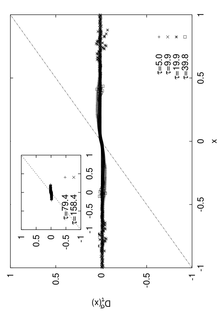
Figure 5: The quantity $D^{\sigma}_{\tau}(x)$ for the phase space contraction rate in a configuration close to equilibrium  $\left({\bf E}=\left(0.1,0.2\right)\right)$.

Figure 6: The quantity $D^{\xi}_{\tau}(x)$ for the entropy production rate in a configuration close to equilibrium  $\left({\bf E}=\left(0.1,0.2\right)\right)$.

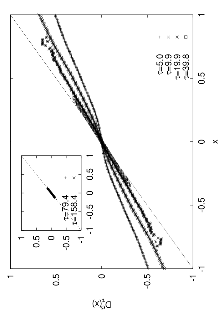
Figure 7: The quantity $D^{\sigma}_{\tau}(x)$ for the phase space contraction rate in a configuration far from equilibrium  $\left({\bf E}=\left(0.8,1.6\right)\right)$.

Figure 8: The quantity $D^{\xi}_{\tau}(x)$ for the entropy production rate  in a configuration far from equilibrium  $\left({\bf E}=\left(0.8,1.6\right)\right)$.

With the measured values of $\Sigma_{\tau}(x)$ and $\Xi_{\tau}(x)$ one can check the FF in this model. In order to visualize the FF we may introduce the quantities

$$D^{\sigma}_{\tau}(x) = \frac{1}{\tau}\,\ln\frac{\Sigma_{\tau}(x)}{\Sigma_{\tau}(-x)}\,,$$ (5)

$$D^{\xi}_{\tau}(x) = \frac{1}{\tau}\,\ln\frac{\Xi_{\tau}(x)}{\Xi_{\tau}(-x)}\,,$$ (6)

which are shown on Fig. 5, 6, 7 and 8. With these quantities Eq. (1) reads as $\lim_{\tau\to\infty}D^{\sigma}_{\tau}(x)=x$ and $\lim_{\tau\to\infty}D^{\xi}_{\tau}(x)=x$. Examining Fig. 5, 6, 7 and 8, one can conclude that

1. For small external forcings and for numerically available $\tau$ values the $\sigma_{\tau}$ fluctuations seem to violate the FF (Fig. 5); this observation is supported by the fact that any symmetric function substituted in Eq. (5) yields zero, and due to the time-reversing symmetry of Eq. (II) the PDF $\Sigma_{\tau}(x)$ is expected to be close to a symmetric function for small external forcings (see Ref. thermsys ).

2. The $\xi_{\tau}$ fluctuations seem to obey the FF both for small and large external forcings.

3. As the external forcing grows, the $\sigma_{\tau}$ fluctuations seem to obey the FF for large $\tau$ values (Fig. 7) similarly to $\xi_{\tau}$ fluctuations.

We note that we have examined several other configurations and have found no significant qualitative differences in the observed behavior of the PDFs.

IV Conclusion

In this paper we have presented numerical evidence showing that the phase-space contraction rate fluctuations violate the fluctuation formula [Eq. (1)] in or close to equilibrium in the Nosé-Hoover thermostated periodic Lorentz gas. This observation is completely in line with the theoretical predictions of Evans et al in Ref. thermsys .

On the other hand, we also demonstrated that the entropy production rate fluctuations satisfy the fluctuation formula, which is by no means trivial. It should also be noted that from the physical point of view the entropy production rate is the more relevant quantity due to its relation to thermodynamics and the availability for measurement in physical experiments. A direct consequence of our results is that the phase-space contraction rate and entropy production rate cannot be treated as interchangeable qunatities in fluctuation formulas, therefore statements regarding the applicability of the FF for various models should always clarify which fluctuations they refer to.

- (1) For a review on the topic see D.J. Evans and D.J. Searles, Adv. Phys. 51, 1529 (2002)
- (2) D.J. Evans, E.G.D. Cohen and G.P. Morriss, Phys. Rev. Lett. 71, 2401 (1993)
- (3) For an overview, see G. Gallavotti, Chaos 8, 384 (1998) and references therein.
- (4) G. Gallavotti and E.G.D. Cohen, J. Stat. Phys. 80, 931 (1995)
- (5) G. Gallavotti and E.G.D. Cohen, Phys. Rev. Lett. 74, 2694 (1995)
- (6) D.J. Evans and D.J. Searles, Phys. Rev. E 50, 1645 (1994), D.J. Evans and D.J. Searles, Phys. Rev. E 52, 5839 (1995), D.J. Evans and D.J. Searles, Advances in Phys.,51, 1529 (2002).
- (7) Giovanni Gallavotti, Lamberto Rondoni and Enrico Segre, Physica D 187, 338 (2004).
- (8) J. Kurchan, J. Phys. A, 31, 3719 (1998)
- (9) D.J. Searles and D.J. Evans, Phys. Rev. E 60, 159 (1999)
- (10) J. L. Lebowitz and H. Spohn,J. Stat. Phys., 95,333 (1999)
- (11) C. Maes, J. Stat. Phys, 95, 367 (1999)
- (12) L. Rondoni, T. Tél and J. Vollmer, Phys. Rev. E 61, 4679 (2000)
- (13) S.Lepri, A. Politi and R. Livi, Physica D 119, 140 (1998)
- (14) Giovanni Gallavotti, Fabio Perroni, e-print chao-dyn/9909007,
- (15) F. Bonetto, G. Gallavotti and P.L. Garrido, Physica D 105, 226 (1997)
- (16) M. Dolowschiák and Z. Kovács, Phys. Rev. E 66, 066217 (2002)
- (17) R. Klages, e-print nlin.CD/0309069 (2003) and E.G.D. Cohen and L. Rondoni, Chaos 8, 357 (1998)
- (18) K. Rateitschak, R. Klages and W.G. Hoover, J. Stat. Phys. 101, 61-77 (2000)
- (19) C.P. Dettmann and G.P. Morriss, Phys. Rev. E 53, 2495 (1996)
- (20) For a review of deterministic thermostats, see R. Klages, e-print nlin.CD/0309069 (2003) and G.P. Morriss and C.P. Dettmann, Chaos 8, 321 (1998)
- (21) Hersir Sigurgeirsson, Andrew Stuart and Wing-Lok Wan, J. Comp. Phys. 172, 766-807 (2001)
- (22) D.J. Evans, D.J. Searles and L. Rondoni, e-print cond-mat 0312353