Temporal chaos versus spatial mixing in reaction-advection-diffusion systems

Abstract

We develop a theory describing the transition to a spatially homogeneous regime in a mixing flow with a chaotic in time reaction. The transverse Lyapunov exponent governing the stability of the homogeneous state can be represented as a combination of Lyapunov exponents for spatial mixing and temporal chaos. This representation, being exact for time-independent flows and equal Péclet numbers of different components, is demonstrated to work accurately for time-dependent flows and different Péclet numbers.

Complex spatiotemporal dynamics has attracted large interest in the last decades. Recently, reaction-diffusion equations have been subject of intense research due to their rich variety of patterns. They describe many important physical systems, such as chemical reactions Kapral and Showalter (1995), lasers Arecchi et al. (1991), or semiconductors Schöll (2001). On the other hand, complex structures can be created in fluid mechanics by spatial mixing Ottino (1989). In this Letter, we consider the combined action of the above effects, leading to a reaction-advection-diffusion system, see Eq. (2) below. Such systems have been investigated with respect to front propagation Abel et al. (2001), excitable dynamics Neufeld et al. (2002), and the filamental structure of reactive particles Toroczkai et al. (2002). Practically, stirred flows with reaction are relevant from large scales (plankton dynamics in the oceans Abraham (1998)) to microscales (construction of a lab on a chip Kneight et al. (1998)), and are important for biophysical, ecological, and chemical applications; similar equations describe the dynamo effect in magnetohydrodynamics Childress and Gilbert (1995).

In this Letter, we consider a temporally chaotic reaction process. It is known that in presence of diffusion, temporal chaos can lead to the appearance of nontrivial spatial structures and space-time chaos. We demonstrate that such structures can appear in the presence of mixing, too. We develop a theory for the transition from spatially homogeneous (fully mixed) temporally chaotic state to a nonhomogeneous one, and compare it with calculations. Our approach is strongly related to the theory of complete synchronization of coupled chaotic systems, which is significantly extended because the spatial mixing leads to special types of coupling.

We now formulate the reaction equations. The evolution of the concentrations $\phi_{i}$, $i=1,\ldots,N$ due to reaction is described by a nonlinear system

$$\frac{d{\phi}_{i}}{dt}=F_{i}(\phi_{1},\ldots,\phi_{N})\;,$$ (1)

with regular or chaotic solutions $\phi^{0}_{i}(t)$. Additionally, each component is subject to diffusion and advection by an incompressible velocity field $\mathbf{v}(\mathbf{r},t)$. Normalization by the characteristic advection time allows a description by dimensionless diffusion constants $d_{i}$ (equivalent to Péclet numbers $d_{i}^{-1}\sim{\rm Pe}_{i}$, generally different) and the dimensionless reaction rate, or Damköhler number, Da. The resulting spatio-temporal equations are

$${\partial\phi_{i}\over\partial t}+(\mathbf{v}\cdot\nabla)\phi_{i}=d_{i}\nabla^{2}\phi_{i}+{\rm Da\,}F_{i}(\phi_{1},\ldots,\phi_{N})\;.$$ (2)

We assume that the concentrations do not influence the flow, so that the field $\mathbf{v}(\mathbf{r},t)$ does not depend on $\phi_{i}$. We supply Eq. (2) with no-flux boundary conditions $\nabla\phi_{i}|_{S}=0$ on the boundary $S$ (periodic boundary conditions are straightforwardly treated in an analogous way).

For a homogeneous spatial distribution of concentrations $\phi_{i}$ the advection and diffusion term vanish and the equations (2) reduce to (1) with rescaled time. To study the stability of spatially homogeneous solutions $\phi_{i}^{0}({\rm Da}\,t)$ of (2) we linearize the equations near this solution and obtain for a small perturbation field $\varphi_{i}(\mathbf{r},t)$

$${\partial\varphi_{i}\over\partial t}+(\mathbf{v}\cdot\nabla)\varphi_{i}=d_{i}\nabla^{2}\varphi_{i}+{\rm Da\,}\,C_{ij}({\rm Da}\,t)\varphi_{j}\;,$$ (3)

where $C_{ij}(t)=\frac{\partial F_{i}}{\partial\phi_{j}}$ is the Jacobi matrix of the system (1) on the solution $[\phi_{1}^{0}(t),\ldots,\phi_{N}^{0}(t)]$. Generally, the solutions of (3) grow or decay exponentially in time $||\varphi||\sim e^{\lambda t}$, where $\lambda$ belongs to the spectrum of Lyapunov exponents (LE). Clearly, the LEs of the solution of (1) belong to this spectrum, describing growth or decay of homogeneous perturbations. The stability of the homogeneous solution towards inhomogeneous perturbations is described by the largest LE corresponding to a spatially varying Lyapunov vector $\varphi(\mathbf{r},t)$ – the transverse LE $\lambda_{\perp}$ [in the sense that it is transverse to a manifold of spatially homogeneous solutions of (3)]. For diffusion constants and time-dependent flow $\mathbf{v}(\mathbf{r},t)$ given, the transverse LE can be determined only numerically. For certain situations, considered below, we obtain this exponent analytically.

We start the analysis of (3) with the simplest case, a time-independent velocity field $\mathbf{v}=\mathbf{v}(\mathbf{r})$ and equal diffusion constants $d_{i}=d$. In this case the ansatz $\varphi_{i}(\mathbf{r},t)=X(\mathbf{r})\Phi_{i}(t)$ allows for a separation of time and space dependence of the perturbation field. The spatial component is determined by the advection–diffusion eigenvalue problem

$$d\nabla^{2}X-(\mathbf{v}\cdot\nabla)X=-\Gamma X,\qquad\nabla X|_{S}=0\;.$$ (4)

The eigenvalue $\Gamma$ describes the decay of non-homogeneous states of the passive scalar field $u(\mathbf{r},t)$, governed by

$${\partial u\over\partial t}+(\mathbf{v}\cdot\nabla)u=d\nabla^{2}u\;,$$ (5)

because for an exponentially time-dependent solution, (5) reduces to (4). This problem has been recently analyzed in Pikovsky and Popovych (2003). The eigenvalue $\Gamma=0$ corresponds to the spatially homogeneous solution and does not contribute to the stability of inhomogeneous perturbations. For the latter, the mode corresponding to the smallest non-zero eigenvalue of (4) is relevant, we denote it by $\gamma$. As has been argued in Pikovsky and Popovych (2003), this eigenvalue crucially depends on the nature of flow $\mathbf{v}(\mathbf{r})$, and thus on Pe. If the flow is mixing, the eigenvalue $\gamma$ is well separated from zero even for small diffusion constant $d$. However, a flow typically contains chaotic and regular domains (islands of Kolmogorov-Arnold-Moser tori). Then, for small diffusion constants, there are weakly decaying modes concentrated in these islands, so that $\gamma$ may be rather small. We notice, that in terms of effective diffusion (coarse grained on the system size $L$) this eigenvalue can be represented as $\gamma=d_{eff}L^{-2}$ Biferale et al. (1995).

The equation for the temporal part $\Phi_{i}$ is

$${d\Phi_{i}\over dt}=-\gamma\Phi_{i}+{\rm Da\,}C_{ij}({\rm Da}\,t)\Phi_{j}$$ (6)

With the ansatz $\Phi_{i}=e^{-\gamma t}w_{i}$ this equation is transformed to the equation for linear perturbations of the reaction problem (1)

$${dw_{i}\over dt}={\rm Da\,}C_{ij}({\rm Da\,}t)w_{j}\;,$$ (7)

its asymptotic solution is $||w||\sim e^{{\rm Da}\lambda t}$, where $\lambda$ is the largest LE of the attractor in (1). Thus, for the perturbation we have $\Phi_{i}\sim e^{({\rm Da}\,\lambda-\gamma)t}$ and the explicit formula for the transverse LE reads:

$$\lambda_{\perp}={\rm Da\,}\cdot\lambda-\gamma({\rm Pe})\;.$$ (8)

The stability condition of the spatially homogeneous state can be formulated as $\lambda_{\perp}<0$. If the oscillations of the concentrations are regular, then the largest Lyapunov exponent is nonpositive $\lambda\leq 0$ and this regime is always stable against spatially inhomogeneous perturbations. A nontrivial transition occurs for a chaotic regime, if $\lambda>0$. Here the stability condition leads to the critical value

$${\rm Da}_{cr}=\frac{\gamma({\rm Pe})}{\lambda}\;.$$ (9)

A similar condition for a trivial case of reaction-diffusion system has been obtained in Pikovsky (1984) and for an abstract mapping model of mixing in Pikovsky (1992). We emphasize that condition (9), obtained for a realistic reaction-advection-diffusion system, can be directly applied to an experiment. Indeed, the eigenvalue $\gamma$ can be directly measured from the time evolution of the contrast of a passive scalar in the flow under investigation Rothstein, Henry, and Gollub (1999). The LE $\lambda$ can be determined from the advection-free setup: the critical domain size $L_{c}$ at which the patterns appear is related to $\lambda$ via $C\,d\,L_{c}^{-2}=\lambda$, where $C$ is a geometrical factor depending on the domain form.

The analysis above is based on simplifying assumptions: time-independence of the velocity field and equality of diffusion constants. In general, if the velocities are time-dependent and the diffusion constants are different, Eq. (3) cannot be simplified and should be analyzed numerically. Since we are interested in stability with respect to spatially inhomogeneous perturbations, the solution should be sought in the class of fields $\varphi$ having zero spatial average (the spatially homogeneous modes in (3) are decoupled from other modes). Numerically, one can use the usual method for calculation of the largest LE: starting with an arbitrary initial field in (3), with vanishing spatial average, one integrates (3) along with (2) performing normalization of the linear field to avoid numerical over- or underflow; averaging the logarithm of the normalization factors yields the transversal LE $\lambda_{\perp}$.

We apply this numerical method to the time-dependent flow, $2\pi$-periodic in space, suggested in Antonsen et al. (1996):

$$\mathbf{v}=\left\{a_{x}f(t)\cos[y+\theta_{x}(t)],\;a_{y}[1-f(t)]\cos[x+\theta_{y}(t)]\right\}.$$ (10)

Here, the simple analytical analysis above is not applicable. Depending on the functions $f(t),\theta_{x}(t),\theta_{y}(t)$, the flow can be time periodic or irregular. In the former case, the particle trajectories demonstrate typical Hamiltonian dynamics with chaotic regions and stability islands (see Antonsen et al. (1996); Pikovsky and Popovych (2003)). A weakly turbulent irregular flow occurs if the functions $f(t),\theta_{x}(t),\theta_{y}(t)$ are random functions of time. We have considered both of these cases with the reaction dynamics (1) given by the Lorenz equations.

An irregular flow was modeled by setting $f(t)$ as a $(0,1)$-telegraph process with independent exponentially distributed time intervals $T_{int}$, and independent uniformly distributed phases $\theta_{x},\theta_{y}\in(0,2\pi)$. The transverse Lyapunov exponent has been calculated as described above; the results are shown in Fig. 1. Remarkably, $\lambda_{\perp}$ is nearly a linear function of Da like in (8). Moreover, we can demonstrate numerically that the formula (8) is valid also quantitatively when all the diffusion constants are equal. To this end, we have calculated the decay rate $\gamma$ from the linear evolution Eq. (5) of the passive scalar. Now this equation does not yield the simple eigenvalue problem (4) because the velocity field is time dependent, but defines in full analogy with the discussion above the asymptotic decay rate $\gamma$ in the sense of the LE (cf. Pierrehumbert (1994)):

$$\gamma=-\lim_{t\to\infty}\frac{\ln||u(\mathbf{r},t)||}{t}\;.$$ (11)

Thus, $\gamma$ is physically interpreted as the asymptotic decay rate of the contrast of the passive scalar in the advection-diffusion problem (5). In Fig. 1, we compare the transverse LE $\lambda_{\perp}$, calculated from (8), with the numerical estimation of $\lambda_{\perp}$. Here, the value of $\gamma$ has been calculated according to (11), $\lambda$ is the largest LE of the Lorenz model; the correspondence with the numerics is within statistical errors. This result indicates that the time dependencies due to chaotic time evolution of species and due to irregularity of the flow are essentially “separable.”

Figure 1: Numerical calculation of transverse LEs from Eqs.  (3) and from approximations (8) and (16). Parameters: $a_{x}=a_{y}=20$, $\langle T_{int}\rangle=0.5$. Squares: $d_{i}=0.1$; circles: $d_{1}=0.1$, $d_{2}=0.2$, $d_{3}=0.5$. Lines are according to (8) and (16).

The analysis above must be modified if the diffusion constants in (3) are different. In this case one has different passive scalar evolution problems Eq. (5), and Eq. (6) is modified to

$${d\Phi_{i}\over dt}=-\gamma_{i}\Phi_{i}+{\rm Da}\,C_{ij}({\rm Da}\,t)\Phi_{j}\;.$$ (12)

The generalized transverse LE for (12) is

$$\Lambda_{\perp}({\rm Da},\gamma_{1},\ldots,\gamma_{N})\;,$$ (13)

for $\gamma_{1}=\ldots=\gamma_{N}=\gamma$ it reduces to (8), but generally cannot be related to the LE of the reaction system like in (7). As a result, instead of (8) and (9), we obtain the following condition for the critical Damköhler number

$$\Lambda_{\perp}({\rm Da}_{cr},\gamma_{1},\ldots,\gamma_{N})=0\;.$$ (14)

There is a connection of the defined above transverse LEs with the theory of synchronization. In the latter one considers two coupled nonlinear systems

$$\begin{array}[]{l}\displaystyle\frac{d{\phi}_{i}^{(1)}}{dt}=F_{i}(\phi_{j}^{(1)})+\frac{\gamma_{i}}{2}(\phi^{(2)}_{i}-\phi^{(1)}_{i})\;,\\[5.0pt] \displaystyle\frac{d{\phi}_{i}^{(2)}}{dt}=F_{i}(\phi_{j}^{(2)})+\frac{\gamma_{i}}{2}(\phi^{(1)}_{i}-\phi^{(2)}_{i})\;,\end{array}$$ (15)

and looks for the stability of the completely synchronized state $\phi_{i}^{(1)}(t)=\phi_{i}^{(2)}(t)$. Then the linearized equation for perturbations coincides with (12). Thus, the generalized transverse LE $\Lambda_{\perp}$ determines the synchronization threshold. This analogy shows that in a stirred reaction the role of coupling constants $\gamma_{i}$ is played by effective decay rates where both advection and diffusion contribute.

In general, some coupling constants can be absent, i.e. the corresponding coefficients $\gamma_{i}$ vanish. In the context of chaotic mixing, such a situation appears, e.g., for surface reactions. Here, it can happen that mobility of some chemical species is large so that they are advected by the fluid flow, while other species are so strongly chemisorb that they cannot move laterally across the surface (see, e.g., Hildebrand et al. (1998)). These chemisorbed species are described by vanishing spatial decay $\gamma_{i}$. In the biological context, mixed and nonmixed components interact, e.g., in marine sediments by tidal flows.

Notice, that although a transformation $\Phi_{i}=e^{-st}W_{i}$ does not allow us to reduce (12) to (7), one parameter, say $\gamma_{N}$, can be eliminated with such a transform. As a result, the generalized transverse LE (13) can be represented as a function of $N-1$ parameters only:

$$\Lambda_{\perp}({\rm Da},\gamma_{i})={\rm Da}\Lambda_{\perp}\left(1,\frac{\gamma_{1}-\gamma_{N}}{{\rm Da}},\ldots,\frac{\gamma_{N-1}-\gamma_{N}}{{\rm Da}},0\right)-\gamma_{N}\;.$$ (16)

In Fig. 2, we show $\Lambda_{\perp}$ for the Lorenz system. The above result for $\Lambda_{\perp}$ agrees well with the direct calculation of transverse LEs for the full system (3), see Fig. 1.

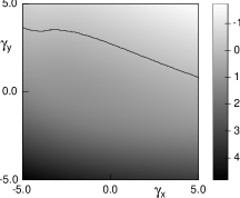
Figure 2: Generalized transverse LEs for the Lorenz model according to (12) with $\gamma_{z}=0$ and ${\rm Da}=1$. The zero contour level is shown with a line.

Above we have performed the stability analysis of the spatially homogeneous regime. Next we discuss properties of structures that appear beyond the stability threshold. A natural quantity to characterize the inhomogeneity of the pattern is the contrast, or variance, $W_{i}=\langle(\phi_{i}-\langle\phi_{i}\rangle)^{2}\rangle$. We solved (2) using (10) with the periodic function $f(t)=(0,1)$ like in Antonsen et al. (1996) with unit period and constant $\theta_{x,y}$, and the Lorenz model as reaction. All three components show the same onset, consistent with linear theory, see Fig. 3. Near the onset of spatial inhomogeneity, the temporal behavior of the pattern contrast is highly intermittent (see inset in Fig. 3). As in a transition to complete synchronization, the reason for this intermittency is the fluctuations of the local exponents $\Lambda_{\perp}$ and $\gamma_{i}$, similar to previously investigated cases Pikovsky (1984); Fujisaka and Yamada (1987).

Figure 3: Time-averaged contrast of the reaction species vs the Damköhler number [the critical value is is 1.096, cf. (9)]. The inset shows temporal intermittency of the contrast $W_{1}$ for ${\rm Da}=1.15$. Parameters: $d_{i}=0.04\cdot\pi^{2}$, $a_{x}=a_{y}=1.2\cdot\pi$.

We have demonstrated that the transition to spatially inhomogeneous structures in a mixed flow with chaotic in time evolution of concentrations is determined by the transverse LE. This exponent can be with good accuracy represented by a sum of “temporal” and “spatial” contributions according to (8), or, more generally, to (16). We can give the following physical arguments in favor of this effective “decoupling” allowing for the separation ansatz. (i) For large Péclet numbers, although different species have different diffusion constants, their mixing properties are to a large extent determined by advection. Thus, one can expect that spatial structures of Lyapunov vectors for different variables $\varphi_{i}(\mathbf{r},t)$ in (3) are close to each other. This is confirmed by numerical simulations: we have calculated the spatial correlation coefficients between different variables for the example presented in Fig. 1 (the case of different diffusion constants) and have found for these correlations the values larger than $0.83$. The same property can be expected for small Péclet numbers, where the spatial structure is given by the purely diffusive version of (4) and one has the same modes for different species, only the decay constants are different. (ii) Although stirring for a time-dependent flow is not constant in time, this seems to have a very small effect on the average transverse LE. We have checked this by solving the generalized system (12) where the decay rates $\gamma_{i}$ are not constants but oscillating functions of time. In some range of periods, the corresponding LE $\Lambda_{\perp}$ remained the same within $1\%$ even if the modulation was as large as $100\%$.

Concluding, we have applied the method of generalized transverse Lyapunov exponents to the analysis of transition from homogeneous to inhomogeneous field in a stirred, temporally chaotic chemical reaction. Our theory is valid for general chaotic reactions and general mixing setups – the latter do not need to be perfect (hyperbolic). For equal diffusion constants, the critical value of the Damköhler number (9) has a clear physical meaning: it determines, whether the growth rate due to temporal chaos (given by the maximal LE of the nonlinear system) wins over the decay rate due to mixing (given by the decay rate of the contrast of a passive scalar in the flow). For different diffusion constants, or for surface reactions where only some species are stirred, the critical Damköhler number can be formulated as a novel problem in the theory of complete synchronization, whose solution is expressed in terms of generalized transverse LEs.

We acknowledge fruitful discussions with B. Eckhardt, O. Popovych, T. Tel, and G. Zaslavsky. A. S. thanks DAAD for support. A. S. and M. A. were supported by the German Science Foundation.

References

- Kapral and Showalter (1995) Chemical Waves and Patterns, edited by R. Kapral and K. Showalter, (Kluwer, Dodrecht, 1995).
- Arecchi et al. (1991) F. T. Arecchi et al., Phys. Rev. Lett. 67, 3749 (1991).
- Schöll (2001) E. Schöll, Nonlinear Spatio-Temporal Dynamics and Chaos in Semiconducters (Cambridge University Press, Cambridge, England, 2001).
- Ottino (1989) J. M. Ottino, The Kinematics of Mixing: Stretching, Chaos, and Transport (Cambridge University Press, 1989).
- Abel et al. (2001) M. Abel et al., Phys. Rev. E 64, 46307 (2001); M. Abel, et al., Chaos 12, 481 (2002); M. Leconte, et al., Phys. Rev. Lett. 90, 128302 (2003).
- Neufeld et al. (2002) Z. Neufeld et al., Phys. Rev. E 66, 066208 (2002);
- Toroczkai et al. (2002) Z. Toroczkai, et al., Phys. Rev. Lett. 80, 500 (1998); Z. Neufeld, C. Lopez, and P. H. Haynes, Phys. Rev. Lett. 82, 2606 (1999); A Focus Issue on Active Chaotic Flows, edited by Z. Toroczkai and T. Tel, [Chaos 12, (2002)].
- Abraham (1998) E. R. Abraham, Nature 391, 577 (1998).
- Kneight et al. (1998) J. B. Kneight et al., Phys. Rev. Lett. 80, 3863 (1998).
- Childress and Gilbert (1995) Stretch, Twist, Fold: The Fast Dynamo, edited by S. Childress and A. D. Gilbert, (Springer, Berlin, 1995).
- Pikovsky and Popovych (2003) A. Pikovsky and O. Popovych, Europhysics Lett. 61, 625 (2003).
- Biferale et al. (1995) L. Biferale et al., Phys. Fluids 7, 2725 (1995).
- Pikovsky (1984) A. S. Pikovsky, Z. Phys. B 55, 149 (1984).
- Pikovsky (1992) A. S. Pikovsky, Phys. Lett. A 168, 276 (1992).
- Rothstein, Henry, and Gollub (1999) D. Rothstein, E. Henry, and J. P. Gollub, Nature (London) 401, 770 (1999).
- Antonsen et al. (1996) T. M. Antonsen et al., Phys. Fluids 8, 3094 (1996).
- Pierrehumbert (1994) R. T. Pierrehumbert, Chaos, Solitons and Fractals 4, 1091 (1994).
- Hildebrand et al. (1998) M. Hildebrand, A. S. Mikhailov, and G. Ertl, Phys. Rev. Lett. 81, 2602 (1998).
- Fujisaka and Yamada (1987) H. Fujisaka and T. Yamada, Prog. Theor. Phys. 77, 1045 (1987).