Resonant enhancement of the jump rate in a double-well potential

Abstract

We study the overdamped dynamics of a Brownian particle in the double-well potential under the influence of an external periodic (AC) force with zero mean. We obtain a dependence of the jump rate on the frequency of the external force. The dependence shows a maximum at a certain driving frequency. We explain the phenomenon as a switching between different time scales of the system: interwell relaxation time (the mean residence time) and the intrawell relaxation time. Dependence of the resonant peak on the system parameters, namely the amplitude of the driving force $A$ and the noise strength (temperature) $D$ has been explored. We observe that the effect is well pronounced when $A/D>1$ and if $A/D\gg 1$ the enhancement of the jump rate can be of the order of magnitude with respect to the Kramers rate.

1 Introduction and the background

In the last decades a lot of interest has been devoted toward the problem of the behaviour of a nonlinear system under the combined influence of stochastic and time-periodic forces. A number of remarkable phenomena such as stochastic resonance (SR) and resonant activation has been discovered and extensively studied both experimentally and theoretically[1, 2, 3]. So far, a lot of experimental confirmations of this effect has been reported in different areas of physics, like optics, biophysics or condensed matter to name a few. In our opinion, the frequency dependence of the SR is one of the most intriguing problem in this area. Initially defined as a problem of “bona fide” stochastic resonance[4], it has created a vivid discussion in scientific literature[5, 4]. The main question in this discussion can be formulated as follows. It is a common knowledge, that the SR phenomenon manifests itself as a maximum of the signal-to-noise ratio (SNR) at the temperature, for which the Kramers rate equals the double driving frequency. However it is not possible to display a similar resonant characteristic as a function of frequency.

On the other hand, experimental observation of the resonant escape from the potential well [6] has stimulated a number of theoretical papers [7, 8]. It has been shown that an underdamped particle driven by both noise and an AC force can perform a resonant escape from the potential well at a certain resonant frequency. However, the narrow resonant peak has been obtained only for underdamped or moderately damped systems, and only recently Pankratov and Salerno in [9] have shown that the mean transition time of an overdamped particle over a periodically oscillating potential well can exhibit a resonant dependence on the frequency of this oscillation in the case of strong (comparing to the depth of the well) driving forces.

The problem we would like to present in this paper is whether an enhancement of the well-to-well transfer (jump) rate is possible in the overdamped bistable system for an arbitrarily strong (or weak) AC force. We believe that the answer to this question is also important because the unperturbed overdamped system does not have oscillatory dynamics, and, therefore does not possess oscillatory frequencies. We are also interested in finding the frequency dependence of the average jump rate for different values of noise and driving amplitude.

2 The model

Consider the overdamped particle in a double-well potential $V(x)$ and under the action of a periodic external force and a white noise. The time evolution of the particle position $x(t)$ is governed by the Langevin equation

$$\gamma\dot{x}=F(x,t)+\xi(t),\;F(x,t)=-V^{\prime}(x)+E(t).$$ (1)

Here the dot stands for differentiation with respect to time, $\gamma$ is the dissipation (damping) parameter, and the double-well potential is chosen as in the $\phi^{4}$ model: $V(x)=(x^{2}-1)^{2}/4$. The relaxation time scale is given by $t_{relax}=2\gamma/V^{\prime\prime}(\pm 1)\equiv\gamma$. The driving force $E(t)=E(t+T)$ has been taken as

$$E(t)=A\tanh{[\mu\sin(\omega t)]}/\tanh{\mu}.$$ (2)

The parameter $\mu$ controls the shape of the function $E(t)$ (see Fig. 1 for details). In the limit $\mu=0$ we obtain simple sinusoidal drive, $E(t)=A\sin(\omega t)$. In the opposite limit, $\mu\rightarrow\infty$, the driving force is of the stepwise form, e.g. $E(t)=+A$ or $-A$ during each of the halfperiods of the driving force.

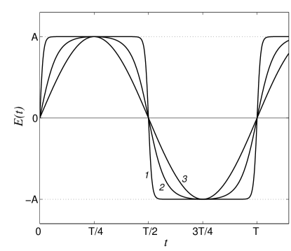
Figure 1: Shape of the driving force $E(t)$ for different values of the parameter $\mu$: $\mu=10$ (curve 1), $\mu=2$ (curve 2) and $\mu=0$ (curve 3).

The importance of the shape of the driving force will be discussed later. The AC force is assumed to be weak, e.g. $A\ll 1$, so that the double-well system does not turn itself into a single-well system during the oscillations of $E(t)$.

The temperature effect is given by a zero-mean stochastic force $\langle\xi(t)\rangle=0$ and auto-correlation function

$$\langle\xi(t)\xi(t^{\prime})\rangle=2D\gamma\,\delta(t-t^{\prime}),$$ (3)

with $D$ being the strength of the noise (dimensionless temperature). Similarly to Eckman and Thomas[10] we are going to characterize the phenomenon by the average number of jumps (or the jump rate) from one well to the other one:

$$\bar{n}=\lim_{\tau\rightarrow\infty}\frac{N_{j}}{\tau},$$ (4)

where $N_{j}$ is the number of jumps during the time interval $\tau$.

In the absence of the periodic driving ($A=0$) the average jump rate is defined by the well-known Kramers formula (see, for example, [11]). Note that for our choice of the potential the height of the barrier is $\Delta V=V(x_{max})-V(x_{min})=1/4$, and, as a result, the Kramers rate equals

$$r_{k}=\frac{1}{\sqrt{2}\pi\gamma}\exp{\left(-\frac{1}{4D}\right)}\left[1-3D/2+{\cal O}(D^{2})\right].$$ (5)

We introduce the amplification factor $\eta$ as a ratio of the average number of jumps in the presence of the driving fields to the jump rate when it is absent: $\eta(\omega)={\bar{n}}(\omega)/r_{k}$. Since it is not possible to solve the corresponding Fokker-Planck equation analytically for all ranges of the driving frequency, we will tackle our problem numerically.

3 Resonant nature of the jump rate

We integrate the corresponding Langevin equation (1) with the Runge-Kutta method and compute numerically the number of particle jumps from one well to another one. We assume that the jumping event took place when the particle had reached the opposite well of the potential. The numerical experiment has been performed during the long times $\tau\gg T=2\pi/\omega,1/r_{k}$, $t_{relax}=\gamma$, so that the time averaging will eliminate any possible dependence on the initial phase.

3.1 Main results of the numerical simulations

Numerical simulations clearly show resonant behaviour of the amplification factor $\eta(\omega)$. In Fig. 2 we show the dependence $\eta$ on the driving frequency for the different values of $A$ and $D$.

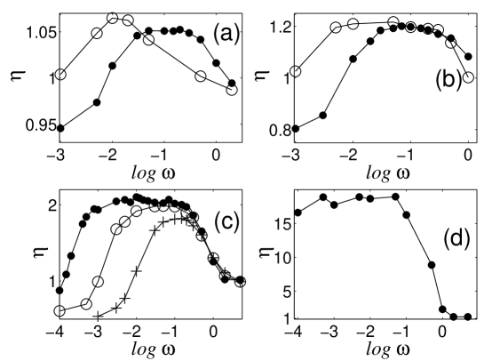
Figure 2: Dependence of amplification of the jump rate $\eta$ on the logarithm of the driving frequency for $\mu=0$, $\gamma=1$, and different ratios $A/D$. Panel (a): $A/D=1/2$; $D=0.04$($\circ$),$D=0.06$($\bullet$). Panel (b): $A/D=1$; $D=0.04$($\circ$), $D=0.06$($\bullet$). Panel (c): $A/D=2$; $D=0.03$($\bullet$), $D=0.04$ ($\circ$), $D=0.06$ ($+$). Panel (d) $A/D=5$, $D=0.02$.

Each of the four panels in the figure corresponds to the certain ratio $A/D$. The resonant nature of the phenomenon can be seen for all values of $A/D$, however it attains considerable values if $A/D\geq 1$. For example, in the panel (d) we present the case of $A/D=5$ where the enhancement can reach the values of $10\div 15$. Note that we did not continue down to the values $\omega<10^{-4}$ since it will require too long averaging times. However, even in the case (d) maximum of the dependence $\eta=\eta(\omega)$ can be seen.

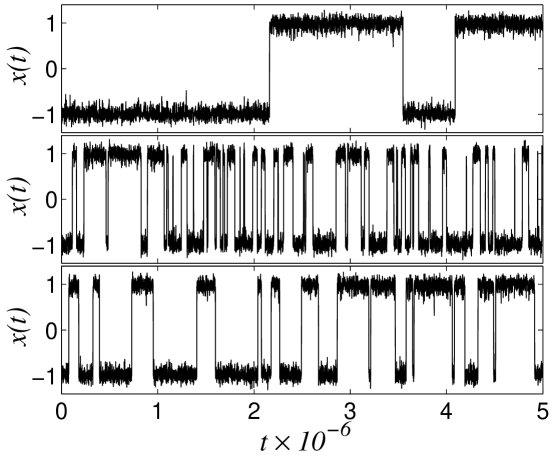
Figure 3: Three examples of time evolution of the dynamic variable $x(t)$ for $\gamma=1$, $\mu=0$, $D=0.02$ at $A=0$, $\omega=0$ (upper panel); $A=0.1$, $\omega=0.001$ (middle panel) and $\omega=0.5$ (lower panel).

Particulars of the dynamics for different values of the driving frequency are shown in Fig. 3. The upper panel shows the time evolution of the particle in the case when no periodic driving force is present. Here jumping events are extremely rare and occur at the rate of order of $r_{k}\sim 8\times 10^{-7}$ [given by the Kramers formula (5)]. The middle panel shows the particle dynamics when the driving frequency equals $\omega=0.001$, that corresponds to the frequencies close to the resonance. Gross enhancement of jumping events is clearly seen. The last panel deals with the case of frequencies much higher than the resonant frequency ($\omega=0.5$ in this case) where the intensity of jumping events is again low.

3.2 Resonance in the jump rate as a switching between different time scales

There are three important time scales in our system: the period of the driving force $T=2\pi/\omega$, the mean residence time in the well, inverse to the Kramers rate, $1/r_{k}$ and the relaxation time of the system, $t_{relax}=\gamma\ll 1/r_{k}$. It is not difficult to see that the dependencies $\eta=\eta(\omega)$, shown in Fig. 2, consist of three distinct parts: (i) $\eta(\omega)$ increases in the adiabatic limit ($\omega\ll r_{k}$) from zero frequencies and continues to grow when $\omega$ exceeds the value of the Kramers rate $r_{k}$; (ii) the plateau in the intermediate area $r_{k}<\omega<1/\gamma$, where the change of $\eta$ is slow and (iii) the high frequency limit, $\omega\gg 1/\gamma$ where $\eta$ decreases with $\omega$ until $\eta$ reaches unity. We shall try to explain the observed resonant enhancement of the jump rate the switching of the above timescales.

First, we try to explain why the jump rate grows in the adiabatic limit. Initially we consider the case of sinusoidal drive ($\mu=0$). In the adiabatic limit $\bar{n}\rightarrow r_{k}$ only for very small driving amplitudes ($A\rightarrow 0$). Momentary escape rates from the lower ($r_{-}$) and upper wells ($r_{+}$) have been calculated in [12]:

$$r_{\pm}(\phi)\simeq r_{k}\xi_{\pm}(A,\phi)\exp\left[\pm\frac{A\sin\phi}{D}\xi_{\pm}(A,\phi)\right],~{}\xi_{\pm}(A,\phi)=1\mp\frac{3A}{4}\sin\phi,$$ (6)

and are, in principle, functions of the the phase $\phi=\omega t$. The momentary residence times $t_{\pm}(\phi)=1/r_{\pm}(\phi)$ obviously also depend on the phase. It is easy to see that for the same phase $\phi$ the increase of the average residence time in the lower well (${\bar{t}}_{-}$) does not compensate the decrease on the average residence time in the upper well (${\bar{t}}_{+}$). In other words, ${\bar{t}}_{-}+{\bar{t}}_{+}\neq 2/r_{k}$, and this “asymmetry” in average residence times must depend on the driving amplitude $A$ in the nonlinear fashion. Using Eq. (6), we show the following:

$$\frac{2}{t_{-}(\phi)+t_{+}(\phi)}=\frac{2r_{-}(\phi)r_{+}(\phi)}{r_{-}(\phi)+r_{+}(\phi)}=r_{k}\frac{(1-\frac{9A^{2}\sin^{2}{\phi}}{16})\exp(-\frac{3A^{2}\sin^{2}\phi}{4D})}{\cosh\left(\frac{A\sin\phi}{D}\right)-\frac{3A\sin\phi}{4}\sinh\left(\frac{A\sin\phi}{D}\right)}.$$ (7)

After some simple manipulations one can obtain that for any physically reasonable values $A$ and $D$ and for any $\phi$ except $\phi=0,\pm\pi$ the expression multiplied by $r_{k}$ in Eq. (7) will be less then $1$. Thus, since the inequality $t_{-}(\phi)+t_{+}(\phi)\neq 2/r_{k}$ holds, the same should hold for the average values: ${\bar{t}}_{-}+{\bar{t}}_{+}\neq 2/r_{k}$. The average number of jumps from well to well can be treated as the inverse mean residence time in the well, $\bar{t}=({\bar{t}}_{-}+{\bar{t}}_{+})/2\equiv 1/\bar{n}$. Strictly speaking, to compute the mean residence times in the upper and lower wells, ${\bar{t}}_{\pm}$, one must perform proper averaging over the phase $\phi$ along the interval $0\leq\phi\leq\pi$. Notice that the greatest contribution to the asymmetry in the jump rates comes from the times when the driving force $E(t)$ attains its extreme values, $t=nT/4$, $n=1,3,5,...$. And, on contrary, at the zeroes of $E(t)$ [$t=nT/2$, $n=0,1,2,...$] the potential is symmetric and their contribution to the asymmetry of residence times is minimal. Thus, the following estimate of the average jump rate (or of the amplification factor $\eta$) is possible:

$$\frac{2}{r_{k}[t_{-}(0)+t_{+}(0)]}=1>\eta>\frac{2}{r_{k}[t_{-}(\frac{\pi}{2})+t_{+}(\frac{\pi}{2})]}=\frac{(1-\frac{9A^{2}}{16})\exp(-\frac{3A^{2}}{4D})}{\cosh\left(\frac{A}{D}\right)-\frac{3A}{4}\sinh\left(\frac{A}{D}\right)}.$$ (8)

Thus we can conclude that $\eta(\omega\rightarrow 0)<1$. Also, it is straightforward to show that $\eta\rightarrow 1$ if $A\rightarrow 0$ and $\eta$ decreases with growth of $A$. This is in accordance with numerical results of Fig. 2, where in panels (a)-(c) it is clearly seen that $\eta<1$ when the driving frequency tends to zero. Also from the numerical results of Fig. 2 one notices that with the growth of the driving frequency the amplification ratio starts to increase. In the adiabatic limit (when $T\rightarrow\infty$) the asymmetry of the residence times in the upper and lower wells is maximal. As long as we increase the frequency (decrease $T$), less jumping events can take place during one driving period. As a result, more often the jumping events will take place around the zeroes of $E(t)$, and, consequently, the contribution of the extreme values of $E(t)$ into the asymmetry between residence times must decrease. This must cause the growth of the jump rate. However, the most remarkable fact is that the amplification ratio $\eta$ does not stop growing when it reaches unity, but continues to increase.

Another limit of our problem is the limit of high driving frequencies $\omega\gg 1/\gamma$. In this case, as opposing to the adiabatic case, a lot of oscillations of the driving force can take place in between the two consecutive jumping events. Thus, the system does not “feel” the AC force on average, and, since $\langle E(t)\rangle_{t}=0$, the influence of the AC drive diminishes. Finally, in the limit $\omega\rightarrow\infty$ the jump rate must tend to the Kramers rate. This is in accordance with previous studies [12, 13] of the resonant escape from the potential well.

Thus, we can conclude that there must exist an optimal driving regime for which the Brownian particle jumps between the wells with the maximal intensity, and this regime must be somewhere in between the adiabatic and high-frequency limits, e.g. in the interval $r_{k}<\omega<1/\gamma$. We have estimated numerically the value of the resonant frequency as $\omega_{res}\simeq(r_{k}/\gamma)^{1/2}$ and this value is much larger then the Kramers rate. In Fig. 4 we investigate this dependence in more detail. In the panel (a) we observe that the maximum of the dependence $\eta=\eta(\omega)$ shifts to the right when $\gamma$ is decreased (while all other parameters are fixed). In the panel (b) we present the behaviour of the resonant frequency $\omega_{res}$ and we see that it does not show any clear dependence on the amplitude.

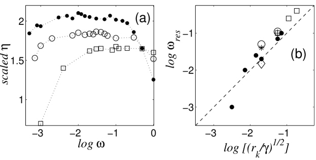
Figure 4: Panel (a). Dependence of the scaled amplification factor on the driving frequency at $A=0.06$, $D=0.03$ and $\mu=0$ for different values of damping: $\gamma=1$ ($\bullet$), $\gamma=0.5$($\circ$), scaled by 90$\%$, and $\gamma=0.1$ (squares), scaled by 80$\%$.
Panel (b). The resonant frequency $\omega_{res}$ as a function of $(r_{k}/\gamma)^{1/2}$ for $A=0.02$ ($\diamond$), $A=0.03$ ($+$), $A=0.04$ ($*$), $A=0.06$ ($\bullet$), $A=0.08$ ($\circ$) and $A=0.1$ (squares). The dashed line is the bisectrix of the straight angle and is shown as a guide to an eye.

Although we do not have a rigorous theory to support such a formula, qualitatively it is easy to understand that this behaviour of the resonant frequency is a result of two competing effects: increasing of the temperature tends to activate the jumping process while damping works against it.

From this estimate of $\omega_{res}$ we see that the resonant frequency is linked with the value of the Kramers rate. Doubling the temperature may increase $\omega_{res}$ by an order of magnitude. Moreover, the steep growth of the curve $\eta(\omega)$ depends solely on the Kramers rate, as it is very clearly demonstrated in Fig. 2c for three different values of $D$ and in Fig. 4a for three different values of $\gamma$. The position of the inflection point in the curve $\eta(\omega)$, which approximately separates the areas of the steep growth and the plateau, moves to the right when the temperature $D$ is increased. This inflection point is always greater then $r_{k}$ but is approximately the same order of magnitude as $r_{k}$. On the other hand, decrease of the dependence $\eta(\omega)$ is controlled only by the damping parameter. It is easy to see that the inflection point which separates the plateau from the high-frequency area does not depend on the temperature. However, it depends strongly on damping $\gamma$ (see Fig. 4) and matches approximately the relaxation frequency $1/t_{relax}=1/\gamma$ (see Figs. 2). This can be explained in the following way: the most probable dynamics is that the particle jumps from the upper well to the lower well. If the time during which the particle moves from one well to another one is of the order of $T/2$, the particle will appear again in the upper well and will perform a jump with a higher probability again. When $\omega$ increases, such synchronization with the relaxation frequency will be lost and if $\omega\gg 1/\gamma$ the particle will have no time to relax in between the oscillations of the potential. Thus, the jumping events will be more rare, the jump rate will decrease. As we enter the high-frequency area the system will react on the external periodic field very weakly. We can conclude that in order to get the maximal jump rate, the frequency of the drive must be synchronized with both the Kramers rate $r_{k}$ and the characteristic relaxation frequency $1/\gamma$.

3.3 Resonant jump rate as a nonlinear response

An important question is how the observed phenomenon depends on the amplitude of the driving force, $A$. In this subsection we show that this dependence has the nature of nonlinear response to the driving force. In principle, there are many ways to demonstrate this. As one example, in Fig. 5 we have plotted the dependence of the amplification factor at its maximal value as a function of the ratio $A/D$ with $D$ being fixed for each of two curves, shown in the figure. Both curves have been fitted

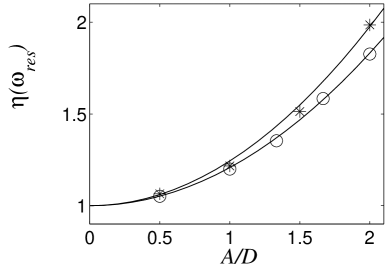
Figure 5: Dependence of the amplification ratio at the resonant value of the driving frequency on the ratio $A/D$ for $\gamma=1$ and $\mu=0$: $D=0.04$ ($*$) and $D=0.06$ ($\circ$). Solid lines are the best fits by the parabolic function (see text for details).

with the parabolic functions. For the case $D=0.04$ we have obtained $1+0.245(A/D)^{2}$ and for $D=0.06$ we have obtained $1+0.21(A/D)^{2}$. Another example which supports the above statement about the nonlinear response is the behaviour of the lower boundary of the amplification ratio $\eta$ in the adiabatic limit [see Eq. (8)]. The expansion of this formula in the powers of $A/D$ yields $1-(17/16)(A/D)^{2}+O((A/D)^{4})$. These results unambiguously show that resonant enhancement of the jump rate can not be described within the framework of the linear response.

3.4 Dependence on the shape of the driving field $E(t)$

Finally we discuss the generality of the obtained results with respect to the shape of the driving force $E(t)$ since the distribution of the residence times $t_{\pm}$ on the initial phase has been omitted when the adiabatic limit has been considered. To check this, numerical simulations have been performed for the two cases of the driving field $E(t)$. In the Fig. 6 we show the dependence of the amplification ratio when the drive is sinusoidal ($\mu=0$) and when it is almost stepwise ($\mu=10$). In the latter case one can assume the distribution of the residence times along the halfperiod of the oscillation of the driving force to be independent on the phase $\phi$. No qualitative differences can be observed for these cases, only the quantitative ones. In the adiabatic limit, the amplification factor is less then one and increases with the growth of the driving frequency regardless of the shape of the driving field $E(t)$.

Another interesting observation is that the maximal amplification of the jump rate depends on the shape of the driving field. We see that for the stepwise shape (large $\mu$) we obtain much better amplification. If $E(t)$ is of the stepwise shape, the time intervals when the potential wells are almost not desymmetrized, are very short. In other words, almost all the time one well is in the uppermost position while another one is in the lowest. The time intervals when the potential is almost symmetric do not contribute anything into the observed resonance, since in that case the jump processes occur with the rate close to $r_{k}$. Thus minimization of these time intervals effectively must enhance the jumps and

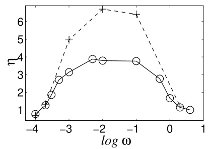
Figure 6: Dependence of the amplification of the jump rate $\eta$ on the logarithm of the driving frequency for $\gamma=1$, $D=0.03$ and $A=0.09$ for different shapes of the driving field $E(t)$: $\mu=0$ ($\circ$) and $\mu=10$ ($+$).

selecting appropriately the shape of $E(t)$ one might increase the amplification significantly. However, this topic is beyond the scope of our paper.

4 Conclusions

To summarize our results, we have found that the jump rate of an overdamped Brownian particle in the double-well potential, driven by a periodic force with zero mean depends resonantly on the frequency of the drive. This phenomenon exists for any ratio of the driving amplitude $A$ to the noise strength, $D$, however is very well pronounced if $A>D$. We also have observed that this phenomenon occurs for different shapes of the driving force $E(t)$. For the stepwise function $E(t)$ the jump rate can be twice larger then in the case of the sinusoidal drive with the same amplitude. An interesting result has been observed in Ref. [14], where diffusion of an overdamped particle in the spatially periodic potential has been studied. The particle is also under the influence of the time-periodic force. Among other results, authors have noticed “acceleration” of diffusion for certain values of the driving period. However, while it was only in the limit $A/D\gg 1$ they observe the effect, in our case it happens for any ratio of $A/D$.

We also would like to mention some analogy of the observed phenomenon with the resonant activation over a fluctuating barrier, which can be driven either randomly as in Ref. [15] or deterministically via periodic force (see Ref. [9]). These papers have shown that the mean first-passage time (MFPT) as a function of the intensity (rate, frequency) of the barrier fluctuations displays a local minimum. In our problem the driving force $E(t)$ effectively induces the oscillating change of the depth of the wells and the average number of jumps $\bar{n}$ is nothing but an inverse MFPT.

Finally we would like to stress the importance of the overdamped case since the dynamics of many biological objects is modeled by overdamped systems, so the above problem could have a wide range of applications.

This work has been supported by the European Union grant LOCNET project no. HPRN-CT-1999-00163. Y. Z. also wishes to acknowledge partial financial support from the Ukrainian Fundamental Research Fund, contract no. 0103U007750.

References

References

- [1] Gammaitoni L et al 1998 Rev. Mod. Phys 70 223-87.
- [2] Anishchenko V S et al, Sov. Phys. Uspekhi 1999 169 7-36.
- [3] Klimontovich Yu L, Sov. Phys. Uspekhi 1999 42 37-44.
- [4] Gammaitoni L, Marchesoni F and Santucci S 1995 Phys. Rev. Lett. 74 1052-5; Choi M H, Fox R F, and Jung P 1998 Phys. Rev. E 57 6335-44; Marchesoni F et al 2000 Phys. Rev. E 62 146-9.
- [5] Zhou T, Moss F and Jung P 1990 Phys. Rev. A 42 3161-9.
- [6] Devoret M H et al 1984 Phys. Rev. Lett. 53 1260-3; Devoret M H et al 1987 Phys. Rev. B 36 58-73.
- [7] Büttiker M, Harris E P, and Landauer R 1983 Phys. Rev. B 28 1268-75; Larkin A I and Ovchinnikov Yu N 1986 J. Low Temp. Phys. 63 317-29; Ivlev B I and Mel’nikov V I 1986 Phys. Lett. A 116 427-8.
- [8] Soskin S M et al 2001 Phys. Rev. E 63 051111.
- [9] Pankratov A L, Salerno M 2000 Phys. Lett. A 273 162-6; Pankratov A L and Salerno M 2000 Phys. Rev. E 61 1206-10.
- [10] Eckman J-P and Thomas L E 1982 J. Phys. A: Math. Gen. 14 3153-68.
- [11] Risken H 1984 The Fokker-Planck Equation (Berlin: Springer-Verlag).
- [12] Jung P, Phys. Rep. 1993 234 175-295.
- [13] Smelyanskiy V N, Dykman M I, and Golding B, Phys. Rev. Lett. 1999 82 3193-7.
- [14] Hu Gang, Daffertshofer A, and Haken H, Phys. Rev. Lett. 1996 76 4874-7.
- [15] Doering C R and Gadoua J C, Phys. Rev. Lett. 1992 69 2318-21.