Existence and characterization of stable ghost orbits in the Hénon map

Abstract

We report a remarkable type of bifurcation: by varying real parameters, unstable complex orbits may become stable over wide parameter ranges. Thus, phase diagrams obtained by analizing solely the stability of real solutions may be incomplete.

The purpose of this paper is to report a remarkable new type of bifurcation: unstable complex orbits may be stabilized by varying real model parameters. In other words, by varying real parameters it is possible to stabilize “complex phases” in phase-diagrams. This surprising fact is shown for the paradigmatic example of a multidimensional dissipative dynamical system, the Hénon map $(x,y)\mapsto(a-x^{2}+by,x)$. The parameter space of the map contains a wide domain of real parameters $a$ and $b$ where it is possible to find complex ‘ghost’ solutions which are stable.

This new bifurcation is of importance in the construction of phase diagrams, usually constructed by sweeping real parameters and studying the set of real solutions, since domains of complex stable motions might be missing in them. Another interesting implication is that the plethora of ghost (complex) orbits, so fundamental nowadays in quite different fields[1, 2, 3], may be subdivided dichotomically into unstable and stable ghosts, pointing to the necessity of investigating the effect of complex stability in all physical applications. In atomic physics, for instance, the stabilization of complex ghost orbits is expected to allow sum re-arrangements in trace formulas[4]. From the exact analytical results reported here one can show that the Hénon map displays Naimark-Sacker bifurcations and, consequently, supports quasiperiodic behaviors[5].

The possibility of stabilizing complex orbits seems not to have been considered before[6, 7], perhaps because the algebraic varieties involved are of very high degrees, exceeding by far those studied by mathematicians[8, 9]. The stabilization of complex orbits was not considered in the classic work of Arnold[10].

As shown recently[11, 12], one may always reduce the equations of motion of any algebraic dynamical systems to a pair of polynomial equations: (i) ${\mathbb{P}}(x,\sigma)=0$, parameterizing simultaneously all orbits of any given period in terms of the sum $\sigma$ of orbital points, and (ii) ${\mathbb{S}}(\sigma)=0$, defining the values of $\sigma$ as a function of model parameters. The degree of ${\mathbb{S}}(\sigma)$ tells the quantity of independent solutions available. In addition, it is also possible to write the secular equation ruling the stability of the system as a function of $\sigma$ and of model parameters. Following Ref. [11], the polynomials providing complete information about all possible period-$6$ orbits are

$${\mathbb{P}}(x,\sigma) = x^{6}-\sigma x^{5}+\theta_{4}(\sigma)x^{4}-\theta_{3}(\sigma)x^{3}+\theta_{2}(\sigma)x^{2}-\theta_{1}(\sigma)x+\theta_{0}(\sigma),$$ (1)

$${\mathbb{S}}(\sigma) = \sum\limits_{i=0}^{9}\ \Theta_{i}(a,b)\sigma^{i},$$ (2)

where $\sigma\equiv x_{1}+x_{2}+x_{3}+x_{4}+x_{5}+x_{6}$ is the sum of the orbital points. The coefficients $\theta_{i}(\sigma)\equiv\theta_{i}(a,b;\sigma)$ are the standard symmetric functions of the roots $x_{\ell}$ (orbital points). The coefficients $\theta_{i}(\sigma)$ and $\Theta_{i}(a,b)$ are given explicitly in the Appendix at the end of the manuscript. Additionally, orbital stability is ruled by the following quadratic for the eigenvalues $\lambda$:

$${\mathbb{L}}(\lambda)=\lambda^{2}-\big{[}2b^{3}+\big{(}\frac{{\mathcal{N}}_{1}+2{\mathcal{N}}_{4}}{{\mathcal{D}}}\big{)}b^{2}-2\frac{{\mathcal{N}}_{5}}{{\mathcal{D}}}b+64\theta_{0}\big{]}\lambda+b^{6}$$ (3)

where ${\mathcal{N}}_{5}$, not contained in Eqs. (1)-(2), is given in the Appendix. Equations (1)-(3) result from quite long algebraic manipulations which were performed automatically on a computer using specially devised ad hoc routines.

The degree of Eq. (2) tells that for any set $(a,b)$ of parameters there are nine possible period-$6$ orbits, not all necessarily different. The actual orbits are found by substituting the nine roots of Eq. (2) into Eq. (1). Since for real parameters all $\Theta_{i}(a,b)$ are real, (i) there is always at least one real value of $\sigma$, and (ii) complex values of $\sigma$ must always appear in conjugate pairs.

Figure 1: Real roots of ${\mathbb{S}}(\sigma)=0$ as a function of $a$, for $b=-0.98$. Stable complex orbits exist between $N_{1}$ and $N_{2}$ on the locus $\sigma_{R}$, the locus of the real root that is always present. PD refers to the period-doubling, $T_{i}$ to tangent bifurcations. The figures on the right show details hard to see on the left. See text.

To get a feeling about the nature of the foliated surface defining $\sigma$ values, Fig. (1) shows the real roots of ${\mathbb{S}}(\sigma)=0$ as a function of $a$, for $b=-0.98$. The four points $T_{i}$ indicate the location of tangent bifurcations. Of special interest is the locus $\sigma_{R}$ defined by that root of Eq. (2) that is always real. Along this locus two different phenomena occur. First, one finds the familiar $3\to 6$ period-doubling bifurcation, indicated by PD. The doubled orbit is stable in a small interval between two vertical dashed lines that is too small to be discernible in the figure. Second, along $\sigma_{R}$ we find a remarkable new type of bifurcation arising from the multivalued character of $\sigma_{R}$ between the points $N_{1}$ and $N_{2}$. In this interval there are three real roots $\sigma$, which define three complex orbits. The complex orbit defined by the “middle branch” interconnecting $N_{1}$ and $N_{2}$, is stable inside a region resembling a “bow-tie” [see Fig. (3) below] precisely where $\sigma_{R}$ displays a fold [in the interval between $N_{1}$ and $N_{2}$ in Fig. (1)] This shows that folds are not always necessarily connected only with tangent bifurcations.

Full lines in Fig. (3) show how the singularities in Fig. (1) evolve when $b$ changes. Dotted lines, obtained by investigating eigenvalues, delimit stability domains in the usual way. For reference, Fig. (3) also displays the interval where period-$1$ orbits (fixed points) are stable. The new bifurcation being reported here occurs inside the box, shown magnified in Fig. (3). As is known, tangent bifurcations may be located analytically from the discriminant of Eq. (2) with respect to $\sigma$.

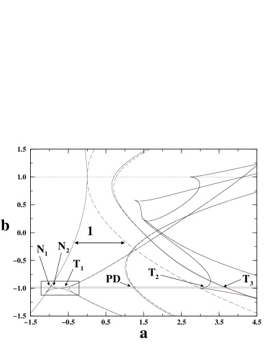
Figure 2: Stability domains and singularities for period-$6$ motions. See text.

Figure 3: Blow-up of the box in Fig. 3. Stable complex orbits exists in $R_{2}$.

Figure (3) shows the stability domain of complex orbits along with a line “1” marking the border where stable orbits of period-$1$ are born when $a$ increases. Recall that physically meaningful solutions exist only in the interval $-1\leq b\leq 1$. The scenario in the region above the line $b=-1$ is divided into four domains labeled $R_{i}$ and displays the following characteristics. All nine period-$6$ orbits are complex in $R_{1}$, despite the fact that one of them corresponds to a real $\sigma$. Moving from $R_{1}$ into $R_{2}$, one finds the complex orbit stabilizing bifurcation, when two additional values of $\sigma$ become real (see curve $\sigma_{R}$ in Fig. (1)) but their corresponding orbits remain complex, one of them being stable. In $R_{3}$ there are three orbits associated with real values of $\sigma$, two orbits being real, one stable and one unstable. The complex orbit is unstable, being the same orbit that will give rise to a stable orbit following the $3\to 6$ period-doubling, when $a$ increases. When moving from $R_{3}$ to $R_{4}$, the stable real orbit looses its stability. The intersection of the “1” line with $R_{2}$, located at $(a_{*},b_{*})\simeq(-0.94832,-0.94764)$, is defined by algebraic numbers of degree $38$, a quite high degree. This intersection has a dual[11] at $b=1/b_{*}\simeq-1.0552$ and $a\simeq-1.0560$. The tip of $R_{2}$, located roughly at $(a,b)=(-0.95449,-0.93348)$, is defined by algebraic numbers of degree $76$.

All in all, the exact expressions reported here, result of long and elaborate algebraic computations, reveal the existence of a new sort of bifurcation that occurs among complex trajectories, transforming unstable ghost orbits into stable complex orbits. Our Eqs (1-3) contain many additional features that will be considered in a future publication[5].

AE is a doctoral fellow of the Conselho Nacional de Desenvolvimento Científico e Tecnológico (CNPq), Brazil. JACG is a Research Fellow of the CNPq. This work was sponsored by CAPES (Brazil) and GRICES (Portugal).

Appendix: The Coefficients $\theta_{i}(a,b;\sigma)$ and $\Theta_{i}(a,b)$

The coefficients $\theta_{i}(a,b;\sigma)$ needed to define all period-$6$ orbits are the following:

$$\theta_{4} = [\sigma^{2}+(1-b)\sigma-6a]/2,$$

$$\theta_{3} = [2\sigma^{3}+6(1-b)\sigma^{2}-32a\sigma-{\mathcal{N}}_{1}(1-b)/{\mathcal{D}}]/12,$$

$$\theta_{2} = (1/24)\{\sigma^{4}+6(1-b)\sigma^{3}-[28a-3(1-b)^{2}]\sigma^{2}-6(1-b)\times$$

$$[4a-(1+b^{2})]\sigma+36[2a-(1+b^{2})]-2(1-b)\sigma{\mathcal{N}}_{1}/{\mathcal{D}}+3b{\mathcal{N}}_{2}/{\mathcal{D}}\},$$

$$\theta_{1} = (1/120)\{\sigma^{5}+10(1-b)\sigma^{4}-5[8a-3(1-b)^{2}]\sigma^{3}-10(1-b)\times$$

$$[10a-3(1+b^{2})]\sigma^{2}+12[22a^{2}-13a(1+b^{2})-2b(1-b)^{2}]\sigma$$

$$-(1-b)[5\sigma^{2}+5(1-b)\sigma-18a]{\mathcal{N}}_{1}/{\mathcal{D}}$$

$$+3[5b\sigma-2(1-b^{3}){\mathcal{N}}_{2}/{\mathcal{D}}-6b{\mathcal{N}}_{3}/{\mathcal{D}}\},$$

$$\theta_{0} = (1/720)\{{\sigma}^{6}+15(1-b){\sigma}^{5}-5[10a-9(1-b)^{2}]{\sigma}^{4}$$

$$-5(1-b)[16a-7{b}^{2}+2b-7]{\sigma}^{3}$$

$$+2[272{a}^{2}-9(27b^{2}-10b+27)a+9(5\,{b}^{2}-8b+5)(1-b)^{2}]{\sigma}^{2}$$

$$+24(1-b)(15a-25{b}^{2}+26b-25)a\sigma-360{a}^{2}(2a-3(1+{b}^{2}))$$

$$-2[(1-b)(5{\sigma}^{3}+15(1-b){\sigma}^{2}-44a\sigma)+15({b}^{4}-b^{3}$$

$$+6{b}^{2}-{b}+1)]{\mathcal{N}}_{1}/{\mathcal{D}}-9[5b{\sigma}^{2}-(1-b)(4{b}^{2}-b+4)\sigma-10ba]{\mathcal{N}}_{2}/{\mathcal{D}}$$

$$+36b\sigma{\mathcal{N}}_{3}/{\mathcal{D}}-360b(1+{b}^{2}){\mathcal{N}}_{4}/{\mathcal{D}}-5(1-b)^{2}({\mathcal{N}}_{1}/{\mathcal{D}})^{2}/2\},$$

where the following abbreviations are used:

$${\mathcal{D}} = 3{\sigma}^{4}-7(1-b){\sigma}^{3}-(12a-11{b}^{2}-5b-11){\sigma}^{2}+(1-b)\times$$

$$(16a-19{b}^{2}-34b-19)\sigma-(1-b)^{2}(4a-8{b}^{2}-13b-8),$$

$${\mathcal{N}}_{1} = {\sigma}^{6}-2(1-b){\sigma}^{5}+2(2a+5{b}^{2}-22b+5){\sigma}^{4}$$

$$-4(1-b)(18a+5{b}^{2}-20b+5){\sigma}^{3}-[32{a}^{2}-8(22{b}^{2}-5b+22)a$$

$$+3(9{b}^{2}+4b+9)({b}^{2}+4b+1)]{\sigma}^{2}+2(1-b)[64{a}^{2}-4(29{b}^{2}+46b$$

$$+29)a+51{b}^{4}+132{b}^{3}+258b^{2}+132b+51]\sigma-12(1-b)^{2}\times$$

$$[8{a}^{2}-(13{b}^{2}+28b+13)a+({b}^{2}+b+1)(8{b}^{2}+13b+8)],$$

$${\mathcal{N}}_{2} = 3{\sigma}^{6}-4(1-b){\sigma}^{5}-12(3a-4b){\sigma}^{4}+2(1-b)(48a+5{b}^{2}$$

$$-26b+5){\sigma}^{3}+[96{a}^{2}-24(7{b}^{2}+3b+7)a+13{b}^{4}+68{b}^{3}+126{b}^{2}$$

$$+68b+13]{\sigma}^{2}-2(1-b)[64{a}^{2}-88(1+b)^{2}a+27{b}^{4}+48{b}^{3}+90b^{2}$$

$$+48b+27]\sigma+4(1-b)^{2}(8a-9{b}^{2}-24b-9)a,$$

$${\mathcal{N}}_{3} = {\sigma}^{7}-2(10a-27b){\sigma}^{5}+2(1-b)(20a-7{b}^{2}-55b-7){\sigma}^{4}+[64{a}^{2}$$

$$-16(8{b}^{2}+11b+8)a+(7{b}^{2}+4b+7)(9{b}^{2}+10b+9)]{\sigma}^{3}$$

$$+2(1-b)[16{a}^{2}+4(29{b}^{2}+53b+29)a-(105{b}^{4}+211{b}^{3}+376b^{2}$$

$$+211b+105)]{\sigma}^{2}-4(1-b)^{2}[48{a}^{2}-(25{b}^{2}+42b+25)a-(8{b}^{2}$$

$$+13b+8)(7{b}^{2}+4b+7)]\sigma+24(1-b)^{3}(4a-8{b}^{2}-13b-8)a,$$

$${\mathcal{N}}_{4} = {\sigma}^{6}-(1-b){\sigma}^{5}-(14a+{b}^{2}-17b+1){\sigma}^{4}+(1-b)(34a-3{b}^{2}$$

$$-43b-3){\sigma}^{3}+[40{a}^{2}-2(29{b}^{2}-b+29)a-4{b}^{4}+27{b}^{3}+8b^{2}$$

$$+27b-4]{\sigma}^{2}-(1-b)[96{a}^{2}-2(69{b}^{2}+110b+69)a$$

$$+16{b}^{4}+87{b}^{3}+178b^{2}+87b+16]\sigma+2(1-b)^{2}\times$$

$$[28{a}^{2}-9(6{b}^{2}+11b+6)a+3({b}^{2}+b+1)(8{b}^{2}+13b+8)],$$

$${\mathcal{N}}_{5} = {\sigma}^{8}+2\,(-9\,a+2\,{b}^{2}+17\,b+2){\sigma}^{6}+2\,(b-1)(-6\,a+9\,{b}^{2}+29\,b$$

$$+9){\sigma}^{5}+(72\,{a}^{2}-12\,(3\,{b}^{2}+22\,b+3)a+186\,{b}^{2}+82\,b+59\,{b}^{4}$$

$$+82\,{b}^{3}+59){\sigma}^{4}+2\,(b-1)[8\,{a}^{2}-12\,(3\,{b}^{2}+16\,b+3)a$$

$$+({b}^{2}+b+1)(111\,{b}^{2}+116\,b+111)]{\sigma}^{3}+2[-32\,{a}^{3}-24\,(2\,{b}^{2}$$

$$-9\,b+2){a}^{2}+(115\,{b}^{4}-56\,{b}^{3}-226\,{b}^{2}-56\,b+115)a+104\,{b}^{6}$$

$$+36\,{b}^{5}+22\,{b}^{4}+22b^{2}+36\,b+104]{\sigma}^{2}+4\,(b-1)[-64\,{a}^{3}$$

$$+4\,(21\,{b}^{2}+62\,b+21){a}^{2}-(11\,{b}^{4}+196\,{b}^{3}+402\,{b}^{2}+196\,b+11)a$$

$$+({b}^{2}+b+1)(16\,{b}^{4}+87\,{b}^{3}+178\,{b}^{2}+87\,b+16)]\sigma$$

$$+8(b-1)^{2}[-24\,{a}^{3}+5\,(11\,{b}^{2}+20\,b+11){a}^{2}-9\,(6\,{b}^{2}+11\,b$$

$$+6)({b}^{2}+b+1)a+3\,(8\,{b}^{2}+13\,b+8)({b}^{2}+b+1)^{2}].$$

The coefficients $\Theta_{i}=\Theta_{i}(a,b)$ needed in Eq. 2 to obtain the $9$ solutions $\sigma_{\ell}=\sigma_{\ell}(a,b)$ are $\Theta_{9}=1$, $\Theta_{8}=1-b$, $\Theta_{7}=-24a+2({b}^{2}+16b+1)$, and

$$\Theta_{6} = 2(1-b)[4a-(7{b}^{2}+12b+7)],$$

$$\Theta_{5} = 144{a}^{2}-16({b}^{2}+25b+1)a+(49{b}^{4}+52{b}^{3}+266{b}^{2}+52b+49),$$

$$\Theta_{4} = -(1-b)[112{a}^{2}-16({b}^{2}+27b+1)a$$

$$+(175{b}^{4}+388{b}^{3}+518{b}^{2}+388b+175)],$$

$$\Theta_{3} = -4[64{a}^{3}-8(b+5)(5b+1){a}^{2}-2(17{b}^{4}-48{b}^{3}-172{b}^{2}$$

$$-48b+17)a-(7{b}^{2}+2b+7)(5{b}^{4}+9{b}^{3}-{b}^{2}+9b+5)],$$

$$\Theta_{2} = 4(1-b)[64{a}^{3}-8(15{b}^{2}+38b+15){a}^{2}+6(23{b}^{4}+48{b}^{3}+96{b}^{2}$$

$$+48b+23)a-(7{b}^{4}+33{b}^{3}+55{b}^{2}+33b+7)(7{b}^{2}+2b+7)],$$

$$\Theta_{1} = 8(1-b)^{2}[32{a}^{3}-2(19{b}^{2}+34b+19){a}^{2}-2(26{b}^{4}+23{b}^{3}+9{b}^{2}$$

$$+23b+26)a+({b}^{2}+b+1)(7{b}^{2}+2b+7)(8{b}^{2}+13b+8)],$$

$$\Theta_{0} = -16a(1-b)^{3}[16{a}^{2}-(37{b}^{2}+62b+37)a+3({b}^{2}+b+1)(8{b}^{2}+13b+8)].$$

References

• [1] P.B. Wilkinson, T.M. Fromhold, R.P. Taylor and A.P. Micolich, Phys. Rev. E, 64 (2001) 026203.
• [2] D. Saraga and T. Monteiro, Phys. Rev. Lett., 81 (1998) 5796-5799.
• [3] S.C. Creagh and N.D. Wheelan, Phys. Rev. Lett., 77 (1996) 4975-79.
• [4] Chaos in Classical and Quantum Mechanics, M.C. Gutzwiller, Springer, New York, 1990.
• [5] A. Endler and J.A.C. Gallas, 2004, to be published.
• [6] S.J. Greenfield, R.D. Nussbaum, J. Diff. Eq., 42 (2001) 57-141.
• [7] O.  Biham, W.  Wenzel, Phys. Rev. A, 42 (1990) 4639-4646.
• [8] Bifurcation Theory and Catastrophe Theory, V.I. Arnold, V.S. Afraimovich, Yu.S. Il’yashenko and L.P. Shilnikov, 2nd printing, 1999, Springer, NY.
• [9] Singularity Theory and Equivariant Symplectic Maps, T.J. Bridges and J.E. Furter, Lecture Notes in Mathematics, vol. 1558, Springer, Berlin, 1993.
• [10] V.I. Arnold, Sov. Phys. Uspheki, 141, 569-590(1983).
• [11] A. Endler and J.A.C. Gallas, Phys. Rev. E, 65 (2002) 036231.
• [12] A. Endler and J.A.C. Gallas, Physica A, 295 (2001) 285-290.