Clustering and collisions of heavy particles in random smooth flows

Abstract

Finite-size impurities suspended in incompressible flows distribute inhomogeneously, leading to a drastic enhancement of collisions. A description of the dynamics in the full position-velocity phase space is essential to understand the underlying mechanisms, especially for polydisperse suspensions. These issues are here studied for particles much heavier than the fluid by means of a Lagrangian approach. It is shown that inertia enhances collision rates through two effects: correlation among particle positions induced by the carrier flow and uncorrelation between velocities due to their finite size. A phenomenological model yields an estimate of collision rates for particle pairs with different sizes. This approach is supported by numerical simulations in random flows.

I Introduction

The dynamics of small impurities, such as droplets, dust or bubbles, transported by an incompressible flow is much more complex than that of point-like fluid tracers. This is due to their finite size and to their mass density being different from that of the carrier fluid. As a consequence of their inertia the dynamics of such particles is dissipative, leading to inhomogeneities in their spatial distribution. This phenomenon, frequently referred to as preferential concentration, has been observed for a long time in experiments (see Ref. EF94, for a review). Suspended particles typically interact through collisions and chemical or biological processes. It is therefore very important in a large spectrum of applications to quantify the effects of inertia on these interactions. Le us mention for instance the problem of estimating the time scales of rain initiation in warm clouds.PK97 ; FFS02 ; Shaw03 Other examples are the problem of microorganism predator-prey encounters in turbulent flows,RO88 ; SF00 ; MOPT02 and the enhancement of chemical reaction rates for active particles suspended in fluid flows.MLG03 ; NTG01 Being a common characteristics of many of the above examples, here we focus on very dilute suspensions of very small particles that are much heavier than the carrier fluid. They are moved by the fluid through a viscous drag, whose nondimensional characteristic time, the Stokes number $S$, is proportional to the square of their radius. In most cases, particle sizes are below the smallest characteristic scale of the flow, where the fluid velocity is spatially smooth. We are interested in the interactions taking place at those scales and we therefore consider random smooth flows.

In the last few years, much effort has been devoted both from a theoreticalST56 ; A75 ; WC83 ; KK96 ; ZSA03 and numericalSC97 ; RC00 ; ZWW01 ; SS02a point of view to understand and quantify the enhancement of collision rates induced by inertia. Two mechanisms have been identified: preferential concentration increases the probability for two particles to be at a colliding distance,RC00 ; FFS02 detachment from fluid trajectories may enhance the relative velocity between two approaching particles.A75 ; KK96 Previous works mostly treated independently these two mechanisms. This is justified in the asymptotics of very small and very large inertia. In the former, particles are almost tracers so that their relative velocity is given by the fluid velocity shear; the discrepancy from a uniform distribution is responsible for an enhancement of collisions. In the other limit particle motion is essentially ballistic: they distribute uniformly but they may reach the same position with very different velocities – this is known as the sling effect.FFS02

Several attempts have been done to bridge the gap between these two asymptotics. For instance, Kruis and KustersKK96 proposed an interpolating formula for the typical particle relative velocity, by summing together the effect of shear due the fluid velocity and the acceleration induced by inertia. This model, though reducing to the result of Saffman and TurnerST56 in the tracer limit and of AbrahamsonA75 for very large inertia, does not take into account the effects of preferential concentration. Some improvements have been proposed in Ref.ZSA03, by using two analytical models for the fluid-particle velocities, but still neglecting the effect of particle clustering.

We propose here a new approach which treats these two mechanisms in a coherent manner. Of course, we do not to provide a complete analytical model for the collision rates, our aim is to introduce a consistent phenomenological framework where the quantities relevant to its estimation are stressed out. We mainly make use of tools borrowed from dynamical systemsER85 to reinterpret inertial effects. The basic idea is to take into account the full position-velocity phase-space dynamics of particles. Preferential concentration of particles is then understood as the convergence of trajectories toward a dynamically evolving attractor in phase space. Folding of the attractor in the velocity direction is responsible for the increase of the velocity differences between particles. The statistical properties of the fractal set are determined by the carrier flow and depend on the particle radius through the Stokes number. This approach has a natural extension to polydisperse suspensions where particles are distributed over sizes: the effects of inertia on the relative motion of particles can there be studied in terms of correlations between attractors labeled by different Stokes numbers.

As we focus on very dilute suspensions, the dynamical effects of collisions are here neglected, i.e. we work within a ghost particle approximation.WWZ98a ; WWZ98b This allows us to investigate the phase space in terms of the Lagrangian dynamics, that is following the trajectories of particle pairs. Thus clustering can be characterized in terms of the probability, $P_{1,2}(r)$, for the pair separation to be below a distance $r$; in the same fashion we introduce the “rate of approach”, defined as the fraction of particle pairs at a distance $r$ that approach each other during a unit time. This is given by the average of the negative part of the radial velocity difference at a separation $r$. As we shall see, the $r$-dependence of these two quantities sheds light on and characterizes the various regimes of particle motion. Moreover, the approaching rate allows to estimate, once $r$ is fixed to be the sum of the particle radii, the collision rates.

In the monodisperse case $P_{1,2}(r)$ behaves as a power law with an exponent displaying a non-trivial dependence on $S$. This exponent is equal to the space dimension, $d$, in both the very small and very large Stokes number asymptotics, where particles distribute uniformly. The scaling behavior of the rate of approach results from the joint effect of clustering and velocity difference between particles. The latter behave very differently in the two asymptotics: for $S\ll 1$ it is proportional to $r$, while for $S\gg 1$ it becomes independent of the separation. For intermediate values of the Stokes number, correlations between particle separations and velocity differences leads to non-trivial scaling behavior for the approaching rate.

As to polydisperse suspensions we show that for the relative motion of two particles with different Stokes numbers, a critical separation $r_{\star}\propto|S_{1}-S_{2}|$ is singled out. Below it, the two motions are essentially uncorrelated. Correlations, due to the fact that particles are suspended in the same flow, show up for length scales above $r_{\star}$. The origin of this characteristic length is understood in terms of the pair-separation dynamics, which is dominated by the Stokes difference for $r<r_{\star}$ (the accelerative mechanism), and by the fluid velocity (the shear mechanism) when $r>r_{\star}$. This crossover length separates in two distinct regimes the scale dependence of both the probability distribution of particle separations and their rate of approach.

Exploiting the phenomenological understanding, supplemented by numerical computation, of the $r$-dependence of the approaching rate (for equal-size and different-size particle pairs) we finally propose a semiquantitative, phenomenological model for the effective collision kernel in polydisperse suspensions.

The paper is organized as follows. In Section II, after recalling the equations of motion, we discuss the basic ingredients and the validity of the approach based on Lagrangian statistics and ghost collisions. In Section III model flows used for numerical illustrations are described. In Section IV and V we investigate the scaling behavior of the pair separation probability and of the approaching rate in monodisperse and polydisperse suspensions, respectively. In Section VI, after a brief review of earlier investigations and models, we propose a phenomenological model for the effective collision kernel in polydisperse suspensions. Section VII is devoted to discussions and conclusions.

II Dynamics and statistics of dilute suspensions

The dynamics of very dilute impurities suspended in an incompressible flow ${\bm{u}}$ is described by a standard model proposed by Maxey and Riley,MR83 which was derived under the following assumptions. The particle radius, $a$, must be much smaller than the Kolmogorov length $\eta$. Particle Reynolds number has to be small enough to ensure that the impurity is surrounded by a Stokes flow. The suspension should be very dilute so that both the hydrodynamical interactions between particles, and their feedback on the carrier fluid can be neglected. Since we focus on the effects induced solely by inertia, we ignore gravity. Here we address the problem of particles much heavier than the carrier fluid, so that this model reduces to the Newton equation:M87

$${d^{2}{\bm{X}}\over dt^{2}}+{1\over\tau}{d{\bm{X}}\over dt}={1\over\tau}{\bm{u}}({\bm{X}},t)\,,$$ (1)

where ${\bm{X}}(t)$ denotes the trajectory. The response time $\tau$, frequently referred to as the Stokes time, is related to the particle radius $a$ by

$$\tau={2\over 9}\,{\rho_{p}a^{2}\over\rho_{f}\nu}\,,$$ (2)

where the mass density ratio between the particle and the fluid $\rho_{p}/\rho_{f}$ is assumed to be very large (e.g. for water droplet in air $\rho_{p}/\rho_{f}\approx 10^{3}$ and for aerosols $\rho_{p}/\rho_{f}\approx 10^{3}-5\times 10^{3}$); $\nu$ is the fluid kinematic viscosity. It is worth reminding that, in the asymptotics of very heavy particles, the prerequisite of small particle Reynolds number does not restrict too much the admissible range for the values of the Stokes time. Indeed the nondimensional Stokes number $S=\tau/\tau_{\eta}=2\rho_{p}a^{2}/(9\eta^{2}\rho_{f})$ (defined as the ratio between the particle response time and the shortest characteristic time scale of the turbulent fluid flow, i.e. the eddy turnover time $\tau_{\eta}$ associated to the Kolmogorov scale) may vary in a range from $0$, the tracer limit, to about $10$ for particle sizes of the order of $\eta/10$ with large mass density ratio.

In terms of the nondimensional parameter $S$, the equation of motion (1) can then be rewritten as

$${d{\bm{X}}\over dt} = {\bm{V}}\,,$$

$${d{\bm{V}}\over dt} = {1\over S}({\bm{u}}({\bm{X}},t)-{\bm{V}})\,,$$ (3)

time being now rescaled by $\tau_{\eta}$. Here, we explicitly introduce the particle velocity ${\bm{V}}$ to emphasize that, at variance with tracers, particle dynamics takes place in the $(2\times d)$-dimensional position-velocity phase space $({\bm{x}},{\bm{v}})$. It should be noted that the dynamics defined by Eq. (3) is uniformly contracting at a rate $-d/S$, so that particle trajectories generally concentrate in phase space onto a dynamically evolving attractor. In the large time asymptotics the phase-space density of particles, solution of the Liouville equation associated to (3), becomes singular with its support on this attractor. Its statistical properties are usually multifractal.ER85

We consider a collection of particles with different Stokes numbers embedded in a flow defined in a finite domain of size $L$. Even though the particles are carried by the same fluid flow, they converge to different attractors according to their Stokes number. A suitable characterization of suspension dynamics is given by the instantaneous phase-space densities $f_{S}({\bm{x}},{\bm{v}},t)$. Here, $f_{S}$ is normalized by the total number of particles with Stokes number $S$, so that it can be interpreted as the probability density to find at time $t$ a particle with Stokes number $S$ at position ${\bm{x}}$ and with velocity ${\bm{v}}$ and for a given fluid flow realization.

In experiments,EF94 one often has access to the distribution of particles in the position space only. The latter is obtained by integrating over particle velocities, $n_{S}({\bm{x}},t)=\int d{\bm{v}}f_{S}({\bm{x}},{\bm{v}},t)$. For tracers, the density $n_{0}({\bm{x}},t)$ is uniformly distributed over the domain, so that the coarse-grained density $\tilde{n}_{0}(r,t)$, obtained by integrating over small volumes of size $r$, scales as $\tilde{n}_{0}(r,t)\sim r^{d}$, being $d$ the spatial dimension. On the contrary, for inertial particles, typically $\tilde{n}_{S}(r,t)\sim r^{D_{1}(S)}$ with $D_{1}$ markedly smaller than the space dimension $d$. The information dimension $D_{1}$ is one among the dimensions $D_{q}$ that characterize the scaling properties of multifractal densities.G83 ; HP83 For particle pairs dynamics the relevant quantity is the correlation dimension $D_{2}(S)$, which measures the scale dependency of the probability $P_{S}(r)$ that two particles on the same attractor are separated by a distance smaller than $r$. Deviations of $D_{2}(S)$ from the value $d$ corresponding to a uniform distribution are important to quantify the weight of clustering (induced by inertia) on particle-to-particle interactions.

The radial distribution function $g(r)$ is frequently used in the literature to characterize clustering of inertial particles.RC00 This quantity can be expressed as the ratio between the actual number of particles inside an infinitesimally thin shell of radius $r$ centered on a given particle and the number that would be expected if the particles were uniformly distributed. It is easily checked that the radial distribution function behaves as $r^{D_{2}(S)-d}$. For particles uniformly distributed, $D_{2}(S)=d$, so that $g(r)\sim{\cal O}(1)$. On the contrary, when $D_{2}(S)<d$, the signature of particle clustering, $g(r)$ diverges as $r\to 0$, as it was numerically demonstrated in Refs. RC00, ; ZWW01, .

It is worth mentioning here that clustering is also found in tracers advected by compressible flows. When the compressibility is sufficiently large, particles can collapse onto point-like attractors: this is usually referred to as the strong compressibility régime.GV00 In such flows, particle inertia may induce a further enhancement of clustering, leading to a strong compressibility régime even at lower values of the compressibility.MW04

Suspensions generally involve local interactions among the particles: dry dust scatters through elastic or inelastic collisions depending on their impact velocitiesWBC01 or water droplets coalesce to form rain drops.FFS02 In dilute suspensions the dominant interactions are the binary collisions taking place when two particles with radii $a_{1}$ and $a_{2}$ (viz. Stokes numbers $S_{1}$ and $S_{2}$), are at a distance $r\approx a_{1}+a_{2}$. It has been proposedWWZ98a ; WWZ98b that for very dilute suspensions, as considered here, the collision rates can be estimated by using the so-called ghost collisions approach. The main idea of this method is to let the particles overlap after they come across a distance equal to the sum of their radii. Neither the particle sizes, nor their velocities are modified after such an event: the collisions are not physically performed but just recorded and counted to estimate the rate at which they happen. To understand the relevance of such an approach let us perform the following gedanken experiment: we throw independently a very large number of particle pairs inside a given domain and let them evolve in different random realizations of the carrier flow until the two particles forming these pairs collide. We define here the collision rate as the rate at which the number of particle pairs which have not collided decreases with time. The dynamics starts with transients during which the probability that two particles collide is strongly influenced, for instance, by the choice of the initial velocities and positions of the particles. When the dynamics of the particles has converged to a statistical steady state, the collision rate attains an asymptotic value which depends on the Stokes numbers of the particles and on the properties of the carrier flow. This limiting value is that measured when assuming ghost collisions. The latter are hence expected to give a good estimate of collision rates in those situations where the time of convergence to a steady régime is much shorter than the mean free time between collisions of particles, as it is for instance the case when considering very diluted suspensions. The framework of ghost collisions have already been compared to several other collision schemes.WWZ98a ; WWZ98b ; RC00b As one could easily expect, it was found to be of particular relevance when the volume fraction of particles is very low. Note finally that beside justifying the use of this approach, the high-dilution hypothesis has another important aspect: it permits to neglect the feedback effect of particles on the fluid flow (the so-called reverse coupling) and to focus on understanding the enhancement of collision rates solely linked to particle inertia.

In order to evaluate collision rates, we introduce the rate at which particles at a distance $r$ approach each other, which can be written in terms of the phase-space densities as

$$\!\!\!\!\kappa_{1,2}(r,t)\!=\left\langle\int_{|\bm{x}_{1}-\bm{x}_{2}|=r}\!\!\!\!\!\!\!\!\!\!\!\!\!\!\!\!\!\!\!d{\bm{\Omega}}_{1}d{\bm{\Omega}}_{2}\,\,f_{S_{1}}(\bm{\Omega}_{1},t)\,f_{S_{2}}(\bm{\Omega}_{2},t)\,w_{1,2}^{-}\right\rangle\,,$$ (4)

where $\bm{\Omega}=(\bm{x},\bm{v})$ and the phase-space integral is performed both on velocities and on positions satisfying $|\bm{x}_{1}-\bm{x}_{2}|=|\bm{r}|=r$, and $w_{1,2}^{-}$ denotes the negative part of the radial velocity difference $({\bm{v}}_{2}-{\bm{v}}_{1})\cdot\hat{\bm{r}}$. The average $\langle[\,\cdots]\rangle$ is performed over the realizations of the fluid velocity field. It easily understood that, for $r=a_{1}+a_{2}$, the rate of approach $\kappa_{1,2}$ gives the fraction of particles of size $a_{1}$ and $a_{2}$ colliding per unit time inside the domain. However, as we shall see, the full $r$-dependence of $\kappa_{1,2}$ is very informative on the dynamics and thus interesting by itself.

The role of inertia in increasing the rate (4) with respect to simple tracers can be understood easily for equal-Stokes particles, $S_{1}=S_{2}=S$. First, the clustering due to inertia enhances the probability for particles to be close to each other. As emphasized in Ref. FFS02, , this mechanism is very important in the asymptotics $S\ll 1$. Second, an additional increase of the rate of approach $\kappa_{1,2}$ may be induced by large radial velocity differences. As a consequence, non-trivial dependencies of $\kappa_{1,2}$ on the scale separation $r$ will emerge. This effect is known to be very important at large $S$, where caustics appear in the phase-space distribution of particles. Such singularities correspond to physical-space positions where a folding of the attractor leads to the presence of different branches in velocity at the same position, and hence, to large velocity differences between close particles. Such a folding in velocity is the basic mechanism leading to what is known as the sling effect.FFS02

Lagrangian statistics

Clearly, a direct $(2\times d)$-dimensional numerical integration to determine phase-space densities is a difficult task. We thus adopt a different strategy by using a Lagrangian approach. Indeed, investigating two-point correlations of densities, as needed for binary collisions, is equivalent to study the relative motion of particle pairs. Moreover the average over velocity configurations can now be replaced by a time average.nota . To evaluate the rate of approach $\kappa_{1,2}$, it is sufficient to follow two particles with Stokes numbers $S_{1}$ and $S_{2}$, and to compute the time average of the negative component of the radial velocity difference conditioned on the pair distance, $r$. Numerically, it is more convenient to condition such averages on having the two particles at a distance smaller than $r$, rather than exactly equal to $r$. This amounts to work with cumulative quantities that are by far less noisy. We hence define

$${\cal K}_{1,2}(r)=\overline{|{W}_{1,2}|\!\!\!\!\phantom{1^{1^{1}}}\!\!H(-{W}_{1,2})\,H(r-{|{\bm{R}}_{1,2}|})}\,,$$ (5)

where ${\bm{R}_{1,2}}={\bm{X}}_{1}-{\bm{X}}_{2}$, ${W_{1,2}}=({\bm{V}}_{1}-{\bm{V}}_{2})\cdot{\bm{R}_{1,2}}/|{\bm{R}_{1,2}}|$, $H$ is the Heaviside function and the overbar denotes Lagrangian time averaging; the rate (4) is then obtained as $\kappa_{1,2}(r)=\partial_{r}{\cal K}_{1,2}(r)$.

To quantify the balance between the two effects enhancing collisions mentioned above, namely clustering and large velocity differences, we make use of the probability density function $p_{1,2}(r)$ for the pair separation. It is clear that this quantity is related to the radial distribution function by $g_{1,2}(r)=L^{d}p_{1,2}(r)/r^{d-1}$. Similarly, instead of measuring directly $p_{1,2}(r)$, we consider the cumulative probability

$$P_{1,2}(r)=\overline{H(r-{|{\bm{R}}_{1,2}\!\!\!\phantom{1^{1^{1}}}\!\!\!\!|})}\,,$$ (6)

that is the probability that two particles are at a distance closer than $r$. It is clear that $p_{1,2}(r)=\partial_{r}P_{1,2}(r)$ (note that while $P_{1,2}$ is adimensional, $p_{1,2}$ has the dimension of the inverse of a length.)

For separations $r$ much smaller than the smallest characteristic length scale of the fluid flow (e.g. the Kolmogorov scale $\eta$ for turbulent flows), both $p_{1,2}$ and $\kappa_{1,2}$ are expected to display power law behaviors:

$$p_{1,2}(r)\sim\left({r\over L}\right)^{\mu(S_{1},S_{2})}\,,$$ (7)

$$\kappa_{1,2}(r)\sim\left({r\over L}\right)^{\gamma(S_{1},S_{2})}\,.$$ (8)

Therefore, the corresponding cumulative quantities $P_{1,2}$ and ${\cal K}_{1,2}$ do also behave algebraically with exponents $\mu+1$ and $\gamma+1$. Note that these quantities are symmetric under particle exchange $(1,2)\mapsto(2,1)$, so that $\mu(S_{1},S_{2})=\mu(S_{2},S_{1})$ and $\gamma(S_{1},S_{2})=\gamma(S_{2},S_{1})$.

For equal-Stokes particles ($S_{1}\!=\!S_{2}\!=\!S$), $\mu(S)\!+\!1$ is exactly the correlation dimension $D_{2}(S)$ of the projection of the attractor onto the physical space. For generic pairs, the exponent $\mu(S_{1},S_{2})+1$ measures the correlation between the distributions of particles of the two types. For smooth flows, the exponent $\gamma$ is constrained between $\mu$ and $\mu+1$. The lower bound is attained when particle velocities and their separation $r$ are uncorrelated, while the upper bound correspond to a velocity difference between particles proportional $r$.

III Model flows

Since collisions occur at distances comparable with the particle radii, therefore typically much smaller than the turbulent viscous scale $\eta$, we can limit ourselves to smooth incompressible fluid velocity fields. In order to perform long time averages at a reasonable cost, we consider synthetic random flows. The physical mechanisms are not expected to be very sensitive to the space dimensionality. The only important effect is that the probability of finding two close particles decreases with the dimension $d$. We therefore choose two-dimensional flows in a finite domain of size $L$. The validity of the results presented in this work should extend, at least qualitatively, to more realistic velocity fields.

First, we consider an isotropic, homogeneous and Gaussian flow. The Fourier modes of the fluid velocity are Ornstein–Uhlenbeck processes satisfying

$${d\hat{\bm{u}}_{\bm{k}}\over dt}=-\frac{1}{\tau_{f}}\hat{\bm{u}}_{\bm{k}}+c_{\bm{k}}\bm{\xi}_{\bm{k}}\,,$$ (9)

where the ${\bm{\xi}}_{\bm{k}}$’s are independent white noises and the correlation time $\tau_{f}$ is independent of the wavevector ${\bm{k}}$. The process (9) is defined over $8$ modes and the constants $c_{\bm{k}}$’s have been suitably chosen to ensure statistical isotropy at small scales. This velocity field, being smooth in space and continuous in time, is expected to mimic the dissipative-range dynamics, when neglecting intermittency effects; $L$ should then be understood as the Kolmogorov scale $\eta$, and the correlation time $\tau_{f}$ as the Kolmogorov time $(\eta^{2}/\epsilon)^{1/3}$. Note that the existence of random dynamical attractors for heavy particles, and hence of a statistically steady state, has been recently proved for this model flow.SS02b The advantage of using a reduced number of modes is that the Fourier summation can be directly performed at particle positions, enabling to resolve the finest scales of the dynamics without interpolation. Particles evolve according to Eq. (1) in a periodic domain of size $L\times L$ (here $L=2\pi$). Time marching is performed by a fourth-order Runge-Kutta scheme for times up to $10^{6}-10^{7}\,\tau_{f}$. The Stokes number is defined as $S=\tau/\tau_{f}$.

Second, we investigate the alternating shear flow:

$$u_{1}\!\! = \!\!0\;;\;u_{2}={U_{n}\,x_{1}(L-x_{1})\over L^{2}}\quad{\mbox{for}}\;\;t\in[{\scriptstyle(n-1)}T,{\scriptstyle(n-{1\over 2})}T]\,,$$

$$u_{1}\!\! = \!\!{U_{n}\,x_{2}(L-x_{2})\over L^{2}}\;;\;u_{2}=0\quad{\mbox{for}}\;\;t\in[{\scriptstyle(n-{1\over 2})}T,{\scriptstyle n}T]\,,$$ (10)

where periodic (of period $L$) boundary conditions are imposed in $(x_{1},x_{2})$, and $U_{n}=\pm U$ is chosen randomly at each time interval $T$ with equal probability. In this case the Stokes number is defined as $S=\tau/T$. The reason for studying such a model flow is twofold. First, it is interesting for testing the robustness of the results, at least at a qualitative level. Second, this model flow has the nice feature that the integration of particle motion can be done explicitly in each time interval of duration $T/2$, allowing for extremely long time averages (up to $10^{8}-10^{9}\,T$).

IV Local dynamics of monodisperse suspensions

We start considering the asymptotics of small Stokes numbers, that is when the particle response time is much smaller than any typical time scale of the flow. A simple perturbative expansion of (3) implies that inertial particles behave as fluid tracers evolving in a slightly compressible flow whose divergence is proportional to $S$.M87 At small separations $r\ll L$, being the carrier flow spatially smooth at these scales, the radial velocity difference of two particles is proportional to $r$. Hence, for equal-size particles $\gamma=\mu+1$. For a vanishing Stokes number $S=0$, the particles behave as tracers in an incompressible flow, therefore they distribute uniformly in space, meaning that $\mu=d-1$ and $\gamma=d$. For small yet finite $S$, if the velocity field is isotropic and homogeneous, one expects the discrepancy from the uniform distribution to behave as $S^{2}$, and in particular $\mu(S)\simeq d-1-\alpha S^{2}$ ($\alpha$ is a flow-dependent constant).BFF01 ; ZA03 In terms of the radial distribution function this means that $g(r)$ diverges in the limit $r\to 0$ as $r^{-\alpha S^{2}}$. This behavior has been indeed observed in Gaussian, random incompressible flowsB03 and in direct numerical simulations of three-dimensional turbulent flows.FP04 Therefore, in the case of small Stokes numbers, the main effects of inertia on particle interactions stems from preferential concentration, which increases the probability of finding close particles.FFS02 ; FP04

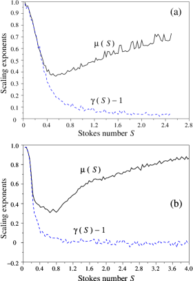
Figure 1: (a) Scaling exponents $\mu$ of the density correlations and $\gamma$ of the rates of approach as a function of the Stokes number for the time-correlated Gaussian random flow. Time averages are performed over $5\times 10^{6}\,\tau_{f}$ (b) Same as in (a) for the shear flow with $T\!=\!L=\!1\,,\,U\!\!=\!\!\sqrt{23}$. Time averages are over $2\!\times\!\!10^{9}\,T$. In both cases the exponents are measured as the mean logarithmic derivative of ${\cal K}$ over two to three decades in $r$.

The other asymptotics is also easy to understand: for $S\gg 1$, particles have a nearly ballistic motion. They are thus expected to distribute uniformly in the whole domain, i.e. $\mu\sim d-1$. Moreover, even close particles have typical velocity differences that do not depend on their separation, i.e. $\gamma\sim\mu\sim d-1$. Therefore, even though in both large and small Stokes numbers asymptotics particle densities are uniform, the rates of approach are markedly different.

The exponents $\mu$ and $\gamma$ computed numerically for the two flows described in Section III are shown in Fig. 1 as a function of the Stokes number $S$. At both small and large values of $S$ the expected behaviors are rather clear: when $S\ll 1$, there is coincidence between $\gamma-1$ and $\mu$ (velocity differences are proportional to the separation), while for $S\gg 1$, one observes that $\gamma\to 2$ (velocities are almost uncorrelated). For intermediate Stokes numbers non-trivial dependencies between particle separations and velocity differences appear. In particular, notice that $\mu$ has a minimum (meaning maximum of clustering) for a finite value of $S$ that, as far as we know, cannot be predicted by any present theory. Moreover, close to this minimum $\gamma-1$ noticeably deviates from $\mu$. As we shall see in Sec. VI, this implies a further increase of the collision rate in this range of Stokes. It is also worth stressing that both models lead to qualitatively similar results, bringing evidence for the robustness of these features. Note that this property Note that this property has already been observed numerically and experimentally.EF94

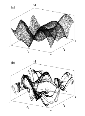
Figure 2: Modulus of the particle velocities as a function of their positions for two different values of the Stokes number (a) $S=10^{-3}$ and (b) $S=1$. At small $S$ the surface identified by the particles velocities is very close to that of the modulus of the Eulerian velocity field, meaning that at fixed spatial position the distribution of the particle velocity is sharply peaked on the fluid one. For larger Stokes numbers, the attractor folds in the velocity direction allowing particles to be very close with very different velocities.

The non-trivial relations between $\gamma$ and $\mu$ at varying $S$ can be understood in terms of two competing effects in phase space: the folding of the attractor in the $\bm{v}$-direction and its tendency to contract toward the surface defined by the instantaneous fluid velocity. The typical rate of this relaxation is given by the Stokes time. For $S=0$ it becomes infinitely fast, preventing folding so that the particle velocity field is mostly mono-valued (see Fig. 2a). As the Stokes number increases the probability of finding particles at the same position with different velocities becomes larger (see Fig. 2b). Such points, once projected onto position space, lead to what can be seen as self-intersections of the attractor projection. This phenomenon was pointed out as the “sling effect” in Ref. FFS02, . We stress that the numerical observations reported in Fig. 1 show that this phenomenon starts to be important already for relatively small Stokes numbers, as signaled by the deviation of $\gamma-1$ from $\mu$.

To summarize, as we expected, the two quantities of interest to measure clustering and collisions have, for particles with the same Stokes number $S$, a power-law behavior at small separations $r$:

$$p_{S}(r) \sim {{\rm C}_{S}\over L}\left({r\over L}\right)^{\mu(S)}\,,$$ (11)

$$\kappa_{S}(r) \sim {{\rm C}_{S}{\rm V}_{S}\over L}\left({r\over L}\right)^{\gamma(S)}\,.$$ (12)

The constant ${\rm C}_{S}$ depends on $S$ and on the statistics of the velocity gradients of the carrier fluid. For three-dimensional turbulent flows it may also depend on the Reynolds number. ${\rm V}_{S}$ is a typical velocity of the particles with Stokes number $S$. For small $S$ it is of the order of the root-mean-square velocity of the carrier flow, $u_{rms}$. For $S\gg 1$ it can be shownZA03 that ${\rm V}_{S}\sim u_{rms}S^{-1/2}$.

V An extension to polydisperse suspensions

We now investigate suspensions with particles having different Stokes numbers. To this aim we consider the equations governing the relative motion of two particles with Stokes numbers $S_{1}$ and $S_{2}$. The separation $\bm{R}$ and the relative velocity $\bm{W}$ evolve according to

$${d{\bm{R}}\over dt} = {\bm{W}}\,,$$

$${d{\bm{W}}\over dt} = {1\over\tau}\,{{\Delta{\bm{u}}-{\bm{W}}}\over 1-{\theta^{2}/4}}-\frac{\theta}{\tau}\,{\bar{\bm{u}}-\bar{\bm{V}}\over 1-{\theta^{2}/4}}\,,$$ (13)

where $\bar{\bm{u}}=({\bm{u}}_{1}+{\bm{u}}_{2})/2$, $\Delta{\bm{u}}={\bm{u}}_{1}-{\bm{u}}_{2}$ and $\bar{\bm{V}}=({\bm{V}}_{1}+{\bm{V}}_{2})/2$. Here and in the sequel, $\tau=(\tau_{1}+\tau_{2})/2$, $S=(S_{1}+S_{2})/2$ and $\theta=(\tau_{1}-\tau_{2})/{\tau}=\Delta S/{S}$.

The two terms in the right-hand side of (13) are associated to different effects. The first corresponds to the relaxation of the relative velocity to the fluid velocity difference. The second is proportional to the difference in Stokes numbers, and therefore it vanishes for equal-size particles. The characteristic length-scale

$$r_{\star}=L|\theta|\,,$$ (14)

distinguishes two ranges of scales. When $R=|\bm{R}|>r_{\star}$, the particle velocity difference is driven by the fluid velocity difference $|\Delta{\bm{u}}|\sim R$ while when $R<r_{\star}$ it is driven by the term originating from the difference in particle response time. As a consequence for $R<r_{\star}$ particle motion is uncorrelated, while above $r_{\star}$ correlations induced by the fact that particles are transported by the same velocity field show up. This mechanism is exemplified in Fig. 3, where the simultaneous snapshots of two populations of particles characterized by different Stokes numbers are shown: at large scales the two distributions look essentially the same, while a closer inspection reveals their differences below the crossover length.

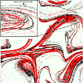
Figure 3: Snapshot of the positions of $N=4\times 10^{5}$ particles associated to two different values of the Stokes number, $S=0.4$ (black) and $S=0.5$ (gray, red online) for the random flow (9). The upper-left inset shows a zoom illustrating the effects induced by the difference in Stokes number (see text for details).

Two cases need to be distinguished: small Stokes number differences, corresponding to $r_{\star}\ll L$ for which an intermediate asymptotic range is present, and finite Stokes number differences for which $r_{\star}\sim{\cal O}(L)$, so that the intermediate range is absent.

a. Small Stokes number differences ($\theta\ll 1$)

In the intermediate asymptotic range $r_{\star}\ll r\ll L$, the particle separation is essentially governed by the first term in (13). The quantities of interest are thus described by the two-point dynamics associated to a single Stokes time – the mean Stokes time. The geometrical interpretation of this dynamical effect is evident from the snapshot of particle positions shown in Fig. 3. Indeed at scales larger than $r_{\star}$ the effects of polydispersion are negligible. In this range of scales we recover the results from the previous Section, namely $p_{1,2}(r)\approx p_{{S}}(r)$ and $\kappa_{1,2}(r)\approx\kappa_{{S}}(r)$ given by (11) and (12), respectively.

As displayed in the inset of Fig. 3 the situation is quite different for $r\ll r_{\star}\ll L$. Now, the time derivative of $\bm{W}$ does not depend on $\bm{R}$, but only on the differential acceleration induced by distinct Stokes numbers. Because of the resulting relative shift between the two attractors in phase space, the velocity difference is independent of the separation. As a consequence, impurities with different $S$ see each other, at such scales, as a gas of uniformly distributed free-streaming particles. This leads to

$$p_{1,2}(r) \sim {{\rm C}_{{S}}\left|\theta\right|^{\mu(S)-d+1}\over L}\left({r\over L}\right)^{d-1}\,,$$ (15)

$$\kappa_{1,2}(r) \sim {{\rm C}_{{S}}\,{\rm V}_{{S}}\left|\theta\right|^{\gamma(S)-d+1}\over L}\left({r\over L}\right)^{d-1}\,.$$ (16)

These expressions match the intermediate asymptotics (11) and (12) for $r=r_{\star}$. The constants ${\rm C}_{{S}}$ and ${\rm V}_{{S}}$ are related to the two-point motion associated to the mean Stokes number ${S}=(S_{1}+S_{2})/2$.

The presence of a characteristic length scale $r_{\star}$ separating these two regimes is confirmed by numerical experiments as shown in Fig. 4.

Figure 4: Rescaled cumulative probability $P_{1,2}(r)$ that two particles are at a distance smaller than $r$ (lower curve), and cumulative approaching rate ${\cal K}_{1,2}(r)$ (upper curve) as a function of $r/r_{\star}$. Results are shown for $S=0.18$ for different values of $\theta$ as in the label. Note the collapse of the different curves; the dashed lines indicate the scaling behavior below and above $r_{\star}$. It is worth also noticing that for $r<r_{\star}$ both $P$ and ${\cal K}$ scale as $r^{2}$ while for $r>r_{\star}$ they scale as $r^{\mu(S)+1}$ and $r^{\gamma(S)+1}$, respectively. As one can see for such a small values of $S$ $\gamma\approx\mu+1$. Data refer to simulations in the random shear flow (10) with $T=1\,,\;L=1\,,\;U=\sqrt{23}$. The curve for $P_{1,2}$ has been shifted down for plotting purposes.

b. Large Stokes number differences ($\theta={\cal O}(1)$)

In this case $r_{\star}$ is of the order of the domain size $L$ and the intermediate asymptotic regime disappears. Therefore, at any scale $r\ll L$ each of the two particles sees the other as if uniformly distributed with independent velocity. The probability that two particles are at a distance $r$ may thus be written

$$p_{1,2}(r)\sim{{\rm C}_{S_{1},S_{2}}\over L}\left({r\over L}\right)^{d-1}\,.$$ (17)

Regarding the rate of approach, the velocity difference can be approximated as the difference between two uncorrelated velocities. This yields to estimate its typical value as $({\rm V}_{S_{1}}^{2}+{\rm V}_{S_{2}}^{2})^{1/2}$, where ${\rm V}_{S_{j}}$ is the characteristic velocity of particles with Stokes number $S_{j}$. It follows

$$\kappa_{1,2}(r)\sim{{\rm C}_{S_{1},S_{2}}\over L}\,\left({\rm V}_{S_{1}}^{2}+{\rm V}_{S_{2}}^{2}\right)^{1/2}\left({r\over L}\right)^{d-1}\,.$$ (18)

VI Phenomenological model for the collision kernel

Let us, for the sake of simplicity, focus on polydisperse suspensions of particles having the same mass density. This assumption implies a one-to-one correspondence between the Stokes number and the particle size, namely $S\propto a^{2}$. In this framework the simplest phenomenological description of particle collisions in dilute suspensions focuses on the total number of collisions per unit time between particles of sizes $a_{1}$ and $a_{2}$ averaged over the fluid velocity realizations:

$${\cal N}_{c}(a_{1},a_{2})=Q(a_{1},a_{2})\,{\cal N}_{1}\,{\cal N}_{2},$$ (19)

where ${\cal N}_{i}$ is the mean number of particles with size $a_{i}$ inside the domain. The effective collision kernel, $Q(a_{1},a_{2})$, is given by the average rate at which particles associated to Stokes number $S_{1}\propto a_{1}^{2}$ and $S_{2}\propto a_{2}^{2}$ arrive at a distance equal to the sum of their radii, i.e. $Q(a_{1},a_{2})=\kappa_{1,2}(a_{1}+a_{2})$. Building quantitative models of the collision kernel in turbulent flows is of utmost importance for many natural phenomena and industrial processes. For instance, we stress that the knowledge of $Q$ is crucial to understand the evolution of the droplet size distribution in clouds,PK97 which is of paramount importance for a theoretical comprehension of the rain drops formation.FFS02 We believe that the main ingredients needed for such a program are, at least at qualitative level, independent on the complexity of the flow. Therefore, here we shall concentrate on the simpler case of random flows, ignoring some (though important) aspects of turbulent flows. Our aim is to develop a semi-quantitative phenomenological model for $Q(a_{1},a_{2})$ able to capture the main ingredients of collisions in suspensions with a broad distribution of particle sizes.

There are two asymptotic regimes where the properties of $Q$ are well understood, namely for vanishing inertia ($S\to 0$) and for infinite response time ($S\to\infty$). As stated in the previous Sections, in both limits particles distribute uniformly, so that investigating the collision kernel reduces to understanding the statistics of velocity differences.

Following Saffman and TurnerST56 , in smooth flows and for $S\to 0$ the collision kernel can be expressed as

$$Q_{ST}(a_{1},a_{2})={\rm D}\,\lambda\,\left(({a_{1}+a_{2}})/L\right)^{d}\,.$$ (20)

This is obtained by multiplying the geometrical cross section $\propto(a_{1}+a_{2})^{d-1}$ with the typical velocity difference between the two particles. The latter is approximated by $\lambda(a_{1}+a_{2})$, being $\lambda$ the characteristic fluid velocity gradient; in turbulent flows the latter is usually estimated as $\lambda\approx(\epsilon/\nu)^{1/2}$.

For $S\to\infty$, it was suggested by AbrahamsonA75 that the kernel can be obtained by a molecular-chaos type of argument, because positions and velocities of particles are uncorrelated:

$$Q_{A}(a_{1},a_{2})=\frac{{\rm D}^{\prime}}{L^{d}}\,\left({\rm V}^{2}_{S_{1}}+{\rm V}^{2}_{S_{2}}\right)^{1/2}\,\left(a_{1}+a_{2}\right)^{d-1}\,,$$ (21)

where ${\rm V}_{S}\sim u_{rms}/S^{1/2}$.

In the last few years most of theoretical efforts focused on the intermediate regime, for which many models and predictions have been proposed. For example, in the regime $S\ll 1$ of very small Stokes numbers, collision rates are enhanced solely by preferential concentration through an increase in the probability of having particles at a colliding distance. This was indeed demonstrated by means of DNS and theoretical analysis.WWZ98b ; RC00 ; BFF01 ; FFS02 ; ZSA03 Thus most of the efforts focused in predicting the net effect of clustering.FP04 This is surely crucial for (close to) monodisperse suspensions of particles with very small sizes, but this approach cannot catch collisions between particles with different sizes. Moreover, even for same-size particles, as soon as the Stokes number reaches small but finite values, inertia besides increasing the probability to find close particles also enhances particle relative velocities. This is clear from Fig. 1 where we see that, as $S$ approaches the value where clustering is maximal, the particle velocity difference is no more proportional to the particle separation. This leads to an additional increase in the collision rates. Indeed, from comparisons with DNS, Wang et al.WWZ00 argued that most models are not able to accurately predict the relative velocity. As to collisions between particles having different sizes the situation is even more involved. Clearly as soon as the Stokes number difference is not negligible the accumulation effect induced by inertia need to be understood in terms of correlations among particle positions belonging to different populations (what we called correlations between different attractors). As far as we know, only few attempts in this direction have been considered. Among them we mention Zhou et al.ZWW01 who investigated by means of DNS, bidisperse suspensions in frozen turbulent flows. In their study they found a reduction of the accumulation effect and an increase in relative velocity. In particular, they proposed a simple model for the particle velocities correlation, in which they prescribed an extremely simplified fluid velocity correlation. Though in fairly good agreement with simulations, their results are rather difficult to interpret because spatial correlations of the fluid velocity are not taken into account. Moreover, their approach seems to be justified only for particle response time of the order of the correlation time of the large scales, $T_{e}$. Indeed, they consider in their numerical simulations particles with response times up to $3T_{e}$. Also Kruis and KustersKK96 proposed a model for bidisperse collisions. In their approach they separate, in a somehow artificial way (as argued in Ref. ZSA03, ), two contributions. The first named shear mechanism corresponds to the carrier fluid velocity shear, that is very similar to the Saffman-Turner result. The second, deriving from the acceleration induced by the different inertia, was called accelerative mechanism. Also this model appear of difficult interpretation due to the absence of spatial correlation in its derivation. Moreover, both mechanisms are considered to be effective simultaneously and the dominance of one over the other is only due to intensity of the velocity gradients, while clearly the particle sizes should play a role too.

In the sequel, exploiting the results obtained in the previous sections, we propose a phenomenological model of the collision kernel which reduces to the known results in the two asymptotics of vanishing and very large Stokes number. In the intermediate regime, an interpolation between the two asymptotics naturally emerges in terms of the exponent $\gamma(S)$ that, (as seen in Fig. 1) out of the two limiting regimes, cannot be trivially related to $\mu$. Moreover, as we shall see, the identification of the crossover scale $r_{\star}$ (14) provides a natural way to discern between differential acceleration and shear mechanisms. To be used for quantitative predictions an analytical estimation of $\gamma(S)$ would be needed. Even for relatively simple random flows, this is far from the present capabilities. However, this quantity is accessible in simulations and may be in principle measured from experiments where particle tracking can be done with a high accuracy.

According to the different cases described in Sec. V, the $(a_{1},a_{2})$ plane has to be divided into different regions corresponding to the various behaviors of $\kappa_{1,2}(r)$ evaluated at $r=a_{1}+a_{2}$. Three regions can be identified (see Fig. 5 for a sketch): region $\bm{A}$ where $r_{\star}\leq a_{1}+a_{2}\leq L$, $\bm{B}$ that is defined by $a_{1}+a_{2}\leq r_{\star}\leq L$, and $\bm{C}$ by $a_{1}+a_{2}\leq L\leq r_{\star}$. Reminding that $r_{\star}\propto|a_{1}^{2}-a_{2}^{2}|/(a_{1}^{2}+a_{2}^{2})$, and the results of Sects. IV and V one has the following behaviors for the collision rates.

$\bm{A}$- In the gray region defined by

$$|a_{1}-a_{2}|\leq 2\,L-\left(4\,L^{2}-(a_{1}+a_{2})^{2}\right)^{1/2}\,,$$ (22)

the behavior of the mean radial velocity difference is well approximated by the two-point motion of particles with the mean Stokes number $S\propto(a_{1}^{2}+a_{2}^{2})$. The collision rate thus reduces to that of particles with the same Stokes number, namely from Eq. (12)

$$Q(a_{1},a_{2})\sim{\rm C}_{S}\,{\rm V}_{S}\,\frac{(a_{1}+a_{2})^{\gamma(S)}}{L^{\gamma(S)+1}}\,,$$ (23)

where the constant ${\rm C}_{S}$ depends on the Stokes number and on the fluid velocity statistics.

$\bm{B}$- In the white region, the inequality (22) is fulfilled, yet it holds

$$|a_{1}-a_{2}|\leq(2-\sqrt{3})\,(a_{1}+a_{2})\,.$$ (24)

The motions of the two particle become uncorrelated and from Eq. (16) one obtains:

$$\!\!\!\!Q(a_{1},a_{2})\sim{\rm C}_{S}\,{\rm V}_{S}\,\frac{|a_{1}-a_{2}|^{\gamma(S)-d+1}\,(a_{1}+a_{2})^{\gamma(S)}}{(a_{1}^{2}+a_{2}^{2})^{\gamma(S)+1}}.$$ (25)

$\bm{C}$- In the hatched region where the inequality (24) is not satisfied, the collision rate is given by

$$\!\!\!\!Q(a_{1},a_{2})\sim{\rm C}^{{}^{\prime}}_{S_{1},S_{2}}\,\left({\rm V}_{S_{1}}^{2}+{\rm V}_{S_{2}}^{2}\right)^{1/2}\,\frac{(a_{1}+a_{2})^{d-1}}{L^{d}}\,,$$ (26)

where ${\rm V}_{S_{1}}$ and ${\rm V}_{S_{2}}$ are the typical velocities associated to particles of size $a_{1}$ and $a_{2}$, respectively. Of course, close to the boundary of the hatched region, the constant ${\rm C}^{{}^{\prime}}_{S_{1},S_{2}}$ should be suitably chosen to ensure continuity of the collision kernel $Q$ in the plane $(a_{1},a_{2})$. Note that this expression is consistent with Abrahamson prediction (21), which is expected to hold for large values of the Stokes number.

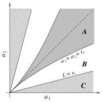
Figure 5: Sketch of the different regions in the $(a_{1},a_{2})$ plane corresponding to different contributions of $\kappa_{1,2}$ to the effective collision rates.

We now make some comments on the different forms taken by the kernel, accordingly to the values of particles sizes. The first obvious information is that Eq. (23) comprises the two asymptotics of very small (20) and very large Stokes numbers (21) when $\gamma$ is replaced by its limiting values. An important observation is that collisions between particles with different Stokes numbers are related to non-trivial scaling behavior only when their radii are rather similar (i.e. in the gray area of Fig. 5). In this region the rates can be obtained in terms of the dynamics for particles with the mean Stokes number. The main information is contained in the Stokes-number dependence of the exponent $\gamma$.

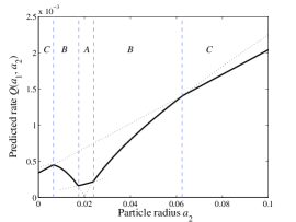
Figure 6: Typical functional shape (bold line) of the collision kernel, represented here as a function of $a_{2}$ through a cut with $a_{1}=0.02$ fixed. We chose here $\gamma=1.8$ and the numerical factors and constants to fit the order of magnitude obtained in our numerical experiments. The effective kernel takes one of the different functional forms (23), (25) or (26) (represented as dotted lines), depending on whether $(a_{1},a_{2})$ is in the region $\bm{A}$, $\bm{B}$ or $\bm{C}$.

According to the predictions (23), (25) and (26) the typical shape of the kernel obtained when fixing one of the radii and varying the other is represented in Fig. 6. The minimal collision rate is obtained for equal-size particles; this is consistent with can be understood from the symmetry of the kernel under particle exchange. The growth of the kernel when $a_{2}\gg a_{1}$ is essentially due to the increase of the geometrical cross-section. Note also the presence of a maximum when $a_{2}<a_{1}$, attained at the crossover between (25) and (26). Note that a similar shape has been proposed for the kernel in Ref. KK96, .

The numerical results for the collision kernel $Q$ in the $(a_{1},a_{2})$ plane are illustrated in Fig. 7 for the Gaussian random flow. The one-dimensional cuts represented in Fig. 8 compare favorably with the prediction shown in Fig. 6. The random shear flow (10) displays similar features (not shown).

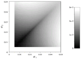
Figure 7: Effective inter-particle collision rate $Q(a_{1},a_{2})$ obtained numerically by considering ghost collisions in the case of the time-correlated random flow. The Stokes number $S$ and the particle radius $a$ are related by $S=2\rho_{p}a^{2}/(9\rho_{f}L^{2})$ with the choice $\rho_{p}/\rho_{f}=4.5\times 10^{3}$. To obtain these rates, inter-particle statistics are computed for 100 different values of the Stokes number.

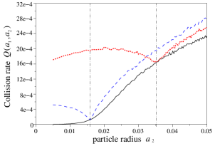
Figure 8: Collision rate $Q(a_{1},a_{2})$ obtained with the same settings as for Fig. 7 and represented here for equal-size particles, i.e. $a_{1}=a_{2}$, (solid curve, black online) and as a function of $a_{2}$ for two fixed values of $a_{1}$: $a_{1}=1.58\times 10^{-2}$ (dashed curve, blue online), (dotted curve, red online) $a_{1}=3.54\times 10^{-2}$.

In order to quantify the importance of particle inertia the ratio $Q(a,a)/Q_{ST}(a,a)$ between the measured kernel and that obtained from of the Saffman–Turner approach (20) is represented in Fig. 9. To disentangle the effects of clustering and densities-velocities correlations, the ratio between the kernel obtained when the velocity difference is assumed to behave linearly with the separation between the two particles, and the Saffman–Turner prediction is represented. Note that the two curves coincide at very small radii: in this regime, the enhancement of collision rates is mainly due to clustering effects. Discrepancies between the two curves appear rather soon, before reaching the maximum of clustering. It is clear from Fig. 9 that in both cases, there is an increase of roughly one order of magnitude in the collision rate of inertial particles compared with that of tracers. However, the measured values of the kernel differ markedly from those obtained when only clustering effects are considered. Therefore, away from the two asymptotics it is crucial not to consider as independent the effects of clustering and enhanced relative velocity.

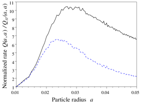
Figure 9: Solid curve (black online): collision rate $Q(a,a)$ for equal-size particles, normalized by that obtained when neglecting particle inertia, i.e. the Saffman and Turner result Eq. (20). Dashed curve (blue online): collision rate obtained when neglecting correlations between the velocity difference and the density (i.e. assuming that the first is just proportional to the separation between the particles), normalized in the same way. These curves were obtained numerically with the same setting as for Fig. 7; the Saffman–Turner kernel was evaluated by following tracer particles advected by the same flow.

VII Concluding remarks

We have identified the main mechanisms leading to the enhancement of clustering and collisions induced by inertia in dilute suspensions of heavy particles. A Lagrangian method based on ghost collisions has been used for numerical investigations. In agreement with previous studies we found that clustering is maximal when the Stokes number is order unity. However, this is not the only mechanism enhancing collisions: large velocity differences can occur at very small separations and for finite values of the Stokes number. This results in non-trivial scaling properties of the rate at which particles come close. A phenomenological model for the collision kernel based on these ingredients has been proposed. Our results highlight the importance of accounting for the full position-velocity phase-space dynamics, particularly for polydisperse solutions. It is important to stress that, away from the small Stokes asymptotics, multiphasic approaches,EAA83 ; CSTC97 based on a continuum description of suspensions in position space, may fail to catch these effects.

We conclude by discussing some aspects concerning impurities in turbulent flows.

We expect our results to be relevant to clustering and collisions at dissipative scales. Turbulence will certainly affect both the values of the constants and the scaling exponents, and induce a non-trivial Reynolds number dependence of the collision rates. Within the framework of model flows it would be interesting to extend the present study to random flows with non-Gaussian statistics to account for intermittency of the velocity gradients. Moreover, in actual turbulent flows the Kolmogorov time-scale is a dynamical variable which has important fluctuations. Therefore, the Stokes number is also a random variable along the particle trajectories. This provides a further complication in developing models accounting for clustering and collisions of particle suspensions, which needs to be investigated.

Another important issue concerns clustering at inertial-range scales, where the velocity field is not differentiable. Experiments indeed show that preferential concentration appears also at those scales.EF94 Non-trivial clustering properties have been observed numerically also in the inverse-cascade range of two-dimensional turbulent flows, namely the formation of holes in the distribution of particles.BLG04 It is important to remark that clustering at the inertial scales may influence the probability for two particles to arrive below the dissipative scale and thus the collision rates. In the inertial range the dynamics of the fluid is close to Kolmogorov 1941 theory, i.e. the velocity field is Hölder continuous with exponent $1/3$. As a consequence, tracers separate explosively giving rise to the celebrated Richardson’s $t^{3/2}$ law. For inertial particles, one needs to understand the competition between explosive separation and clustering due to dissipative dynamics. In this direction, it may be useful to further extend to inertial particles recent models and techniques developed in the framework of passive scalars (for two recent reviews see Refs. SS00, ; FGV01, ).

References

- (1) J.K. Eaton and J.R. Fessler, “Preferential concentrations of particles by turbulence,” Int. J. Multiphase Flow 20, 169 (1994).
- (2) M.B. Pinsky and A.P. Khain, “Turbulence effects on droplet growth and size distribution in clouds- a review,” J. Aerosol Sci. 28, 1177 (1997).
- (3) G. Falkovich, A. Fouxon, and M.G. Stepanov, “Acceleration of rain initiation by cloud turbulence,” Nature 419, 151 (2002).
- (4) R.A. Shaw, “Particle-turbulence interactions in atmospheric clouds,” Ann. Rev. of Fluid Mech. 35, 183 (2003).
- (5) B.J. Rothschild and T.R. Osborn, “Small-scale turbulence and plankton contact rates,” J. Plankton Res. 10, 465 (1988).
- (6) S. Sundby and P. Fossum, “Feeding conditions of arcto-nowegian cod larvae compared with the Rothschild-Osborn theory on small-scale turbulence and plankton contact rates,” J. Plankton Res. 12, 1153 (2000).
- (7) J. Mann, S. Ott, H.L. Pécseli and J. Trulsen, “Predator-prey enconunters in turbulent waters,” Phys. Rev. E 65, 026304 (2002).
- (8) A.E. Motter, Y.-C. Lai and C. Grebogi “Reactive dynamics of inertial particles in nonhyperbolic chaotic flows,” Phys. Rev. E 68, 056307 (2003).
- (9) T. Nishikawa, Z. Toroczkai and C. Grebogi, “Advective coalescence in chaotic flows,” Phys. Rev. Lett. 87, 038301 (2001).
- (10) P.G. Saffman and J.S. Turner, “On the collision of drops in turbulent clouds,” J. Fluid Mech. 1, 16 (1956).
- (11) J. Abrahamson, “Collision rates of small particles in a vigorously turbulent fluid,” Chem. Eng. Sci. 30, 1371 (1975).
- (12) J.J.E. Williams and R.I. Crane, “Particle collision rate in turbulent flow,” Int. J. Multiphase Flow 9 421, (1983).
- (13) F.E. Kruis and K.A. Kusters, “The collision rate of particles in turbulent Media,” J. Aerosol Sci. 27, Supplement 1 , S263 (1996).
- (14) L.I. Zaichik, O. Simonin and V. Alipchenkov, “Two statistical models for predicting collision rates of inertial particles in homogeneous isotropic turbulence,” Phys. Fluids 15, 2995 (2003).
- (15) S. Sundaram and L.R. Collins, “Collision statistics in an isotropic, particle-laden turbulent suspensions”, J. Fluid Mech. 335, 75 (1997).
- (16) W.C. Reade and L.R. Collins, “Effect of preferential concentration on turbulent collision rates,” Phys. Fluids 12, 2530 (2000).
- (17) Y. Zhou, A.S. Wexler and L.-P. Wang, “Modelling turbulent collision of bidisperse inertial particles”, J. Fluid Mech. 433, 77 (2001).
- (18) H. Sigurgeirsson and A.M. Stuart, “A model for preferential concentration,” Phys. Fluids 14, 4352 (2002).
- (19) J.-P. Eckmann and D. Ruelle, “Ergodic theory of chaos and strange attractors,” Rev. Mod. Phys. 57, 617 (1985).
- (20) L.-P. Wang, A.S. Wexler and Y. Zhou, “On the collision rate of small particles in isotropic turbulence. Part I. Zero-inertia case,” Phys. Fluids 10, 266 (1998).
- (21) Y. Zhou, L.-P. Wang and A.S. Wexler, “On the collision rate of small particles in isotropic turbulence. Part II. Finite-inertia case,” Phys. Fluids 10, 1206 (1998).
- (22) M.R. Maxey and J. Riley, “Equation of motion of a small rigid sphere in a nonuniform flow,” Phys. Fluids 26, 883 (1983).
- (23) M.R. Maxey, “The gravitational settling of aerosol particles in homogeneous turbulence and random flow fields,” J. Fluid Mech. 174, 441 (1987).
- (24) P. Grassberger, “Generalized dimensions of strange attractors,” Phys. Lett. A 97, 227 (1983).
- (25) H.G.E. Hentschel and I. Procaccia, “The infinite number of generalized dimensions of fractals and strange attractors,” Physica D 8, 435 (1983).
- (26) K. Gawȩdzki and M. Vergassola, “Phase Transition in the Passive Scalar Advection,” Physica D 138, 63 (2000).
- (27) B. Mehlig and M. Wilkinson, “Coagulation by random velocity fields as a Kramers problem,” Phys. Rev. Lett. 92, 250602 (2004).
- (28) G. Wurm, J. Blum and J.E. Colwell, “Aerodynamical sticking of dust aggregates,” Phys. Rev. E 64, 046301 (2001).
- (29) W.C. Reade and L.R. Collins, “A numerical study of the particle size distribution of an aerosol undergoing turbulent coagulation,” J. Fluid Mech. 415, 45 (2000).
- (30) This requires to assume ergodicity for the particle dynamics, which is usually the case.
- (31) H. Sigurgeirsson and A.M. Stuart, “Inertial particles in a random field,” Stoch. and Dyn. 2, 295 (2002).
- (32) E. Balkovsky, G. Falkovich and A. Fouxon, “Intermittent distribution of inertial particles in turbulent flows,” Phys. Rev. Lett. 86, 2790 (2001).
- (33) L.I. Zaichik and V. Alipchenkov, “Pair dispersion and preferential concentration of particles in isotropic turbulence,” Phys. Fluids 15, 1776 (2003).
- (34) J. Bec, “Fractal clustering of inertial particles in random flows,” Phys. Fluids 15, L81 (2003).
- (35) G. Falkovich and A. Pumir, “Intermittent distribution of heavy particles in a turbulent flow,” Phys. Fluids 16, L47 (2004).
- (36) L.-P. Wang, A.S. Wexler and Y. Zhou, “Statistical mechanics description and modeling of turbulent collision of inertial particles,” J. Fluid Mech. 415, 117 (2000).
- (37) S.E. Elghobashi and T.W. Abou-Arab, “A two-equation turbulence model for two-phase flows,” Phys. Fluids 26, 931 (1983).
- (38) C.T. Crowe , M. Sommerfeld , Y. Tsuji and C. Crowe, “Multiphase flows with droplets and particles,” CRC Press (1997).
- (39) G. Boffetta, F. De Lillo and A. Gamba “Large scale inhomogeneity of inertial particles in turbulent flows,” Phys. Fluids 16, L20 (2004).
- (40) B.I. Shraiman and E. Siggia, “Scalar turbulence,” Nature 405, 639 (2000).
- (41) G. Falkovich, K. Gawȩdzki and M. Vergassola, “Particles and fields in fluid turbulence,” Rev. Mod. Phys. 73, 913 (2001).