Oscillating kinks in forced oscillatory media: A new type of instability

Abstract

A new type of instability resulting in oscillatory propagating kinks is presented. It is observed in periodically forced oscillatory media at 1:1 resonance, where phase kinks have close similarities to pulses in excitable media. Considering the periodically forced complex Ginzburg-Landau equation, examples for transitions involving oscillating kinks between different dynamical regimes are described. The oscillatory instability is discussed within the framework of a bifurcation analysis of the kink profiles.

I Introduction

In many cases, synchronization and desynchronization turned out to be the underlying mechanisms for transitions between ordered states and complex behavior in spatially extended systems Pikovsky et al. (2001). Systems with local oscillatory dynamics, e.g., chemical reactions like the Belouzov-Zhabotinsky reaction, are sensitive to external driving Kapral and Showalter (1995); Petrov et al. (1997). Such systems may be synchronized by external forcing or global feedback. It has been demonstrated both theoretically and in experiment that these methods provide powerful tools to control pattern formation in various systems Coullet and Emilsson (1992a, b); Battogtokh and Mikhailov (1996); Battogtokh et al. (1997); Kim et al. (2001); Bertram and Mikhailov (2003); Bertram et al. (2003a, b).

Detailed studies have been carried out about synchronization phenomena in 1-D geometries Chaté et al. (1999); Braiman et al. (1995); Elphick et al. (1999). It turned out that in the presence of external forcing as well as under global feedback, localized pulses, so-called phase kinks or phase flips, may appear Falcke and Engel (1997); Mertens et al. (1993). These objects deserve special interest, since they illustrate the similarities in the behavior of forced oscillatory media on the one hand and and excitable systems on the other hand. Coullet first pointed out that these phase kinks behave like pulses in excitable media Coullet and Emilsson (1992a, b).

These pulses or phase kinks can undergo an instability leading to self-replication. Then, spatiotemporal intermittency Chaté and Manneville (1987) can be observed and characteristic Sierpinski gasket-looking patterns are possible Hayase and Ohta (1998). Such patterns seem to be ubiquitous in a wide range of systems. They have been reported in reaction–diffusion systems Lee et al. (1994); Lee and Swinney (1995), fluid drag experiments Vallette et al. (1997), pigmentation dynamics on sea shells Meinhardt (2003), and dynamics of membrane voltage Keener and Sneyd (1998). In Argentina et al. (2004), a mechanism leading to those patterns has been described in terms of geometrical arguments.

Here, a new type of instability is presented. It is an oscillatory instability and results in pulses propagating at constant average velocity with periodically varying shape.

II Model

In this work, synchronization is studied in a 1-D spatially distributed system close to the onset of an oscillatory instability at frequency $\omega_{\rm 0}$. A qualitative description of such systems is provided by the complex Ginzburg-Landau equation Aranson and Kramer (2002); Cross and Hohenberg (1993)

$$A_{t}=A-(1+i\alpha)|A|^{2}A+(1+i\beta)A_{xx}.$$ (1)

$A(x,t)$ is the complex amplitude of the oscillations. The parameter $\alpha$ describes the nonlinear frequency shift, $\beta$ accounts for the dispersion of the medium. Depending on $\alpha$ and $\beta$, Eq. (1) shows different types of dynamics. If $1+\alpha\beta<0$, two kinds of disordered dynamics are observed: phase turbulence [$|A|>0$ for all $(x,t)$] and defect turbulence ($|A|=0$ for certain points in the $x$-$t$ plane, so-called space-time defects). In the region $1+\alpha\beta>0$, some plane wave solutions are linearly stable. Under certain conditions, patches of stable plane wave solutions with different wavelengths coexist separated by localized propagating objects. Such a state is called spatiotemporal intermittency (STI).

In the presence of a spatially homogeneous harmonic forcing, $F(t)=B\exp(i\omega_{\rm e}t)$, the above mentioned states may synchronize. This can be modeled with the forced complex Ginzburg-Landau equation. Using a coordinate frame rotating with the external forcing [$A\to\Psi\equiv A\exp(-i\omega_{\rm e}t)$], one obtains an autonomous equation with an additive forcing term, $F_{n}=B^{n}(\Psi^{\ast})^{n-1}$, if the detuning $\nu=\omega_{\rm 0}-m/n\omega_{\rm e}$ is sufficiently close to zero Coullet and Emilsson (1992a, b). Here the 1:1 resonance ($n=m=1$) is considered and the equation reads

$$\Psi_{t}=(1+i\nu)\Psi-(1+i\alpha)|\Psi|^{2}\Psi+(1+i\beta)\Psi_{xx}+B\;.$$ (2)

Depending on $B$ and $\nu$, the oscillations in the system can completely synchronize with the external forcing, resulting in a stationary spatially homogeneous state $\Psi(x,t)\equiv\Psi_{0}$. However, this is not the only possible synchronized state. The fixed point state $\Psi_{0}$ can be the background for localized phase jumps of $2\pi$, so-called phase kinks or phase flips Coullet and Emilsson (1992a, b); Chaté et al. (1999) (Fig. 1).

Figure 1: Spatial profiles of a propagating phase kink for $\alpha=-0.75$, $\beta=1.8$, $\nu=-0.758$, $B=0.015$. Right: phase, center: modulus $|\Psi|$, left: real part $Re(\Psi)$.

They can undergo an instability leading to the destruction of a kink in a space-time defect. This can give rise to different dynamical regimes Chaté et al. (1999) (Fig. 2).

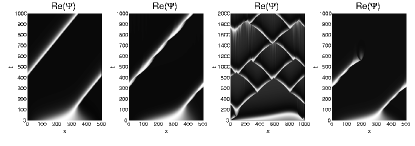
Figure 2: Four typical spatiotemporal diagrams of the real part of $\Psi$. From left to right: stable propagating kink, oscillatory propagating kink, kink replication, destruction of a kink.

Stable kinks propagating at constant velocity $V$ are stationary solutions of

$$\Psi_{t}=(1+i\nu)\Psi-(1+i\alpha)|\Psi|^{2}\Psi+(1+i\beta)\Psi_{xx}+B-V\Psi_{x}\,.$$ (3)

They can be described in a comoving frame $\xi=x-Vt$. Then Eq. (2) reduces to a system of four coupled ODEs (traveling wave ODEs). The homogeneous state $\Psi_{0}$ corresponds to a saddle fixed point with two-dimensional stable and unstable manifolds. A phase kink is a homoclinic connection between these manifolds. It is of codimension one and thus exists only for certain values of $V$. Kink profiles can be computed numerically by continuing these homoclinic orbits in the traveling wave ODEs, e.g., using AUTO97/2000 Beyn et al. (2002). Such an analysis shows that stable and unstable kink profiles usually coexist Argentina et al. (2004). A linear stability analysis for a kink profile $\Psi_{V}$ can be done by inserting $\Psi_{V}$ into the linearized Eq. (3) and computing the eigenvalues.

III Oscillating propagating kinks

Numerical simulations indicate that preferably at higher values of the dispersion coefficient $\beta$, phase kinks can undergo a new type of instability leading to oscillatory propagating kinks. Here Eq. (2) is considered for $\alpha=-0.75$ and $\beta=1.8$, when the CGLE without forcing exhibits phase turbulence. In this section, two examples of scenarios leading to oscillating kinks are discussed. In both cases, $B$ is fixed and the detuning $\nu$ is varied. One scenario is connected to the transition from stable kinks to STI, the other can be observed at higher values of $B$, when a transition from stable kinks to a homogeneous state without kinks takes place.

III.1 Example 1: Oscillating kinks at the transition to STI

Let us consider the situation at $B=0.015$. For $\nu>\nu_{\rm sn}-0.75858$, only stable propagating kinks can be observed. If we decrease $\nu$, stable propagating kinks are still possible. However, depending on the initial conditions, numerical simulations show a new phenomenon: After a transient, the spatial profile evolves to a kink profile with a periodically changing shape propagating at constant average velocity. For $\nu<\nu_{\rm H}=-0.76081$, any initial condition with a phase rotation of $2\pi$ evolves to such an oscillatory propagating kink; no stable kinks are possible. At $\nu_{\rm kr}=-0.76598$, a transition to kink replication takes place. The coexistence of stable and oscillatory kink profiles leads to hysteresis behavior. Starting with a stable kink at $\nu>\nu_{\rm sn}$, it persists, if $\nu$ is slowly decreased to $\nu_{\rm H}<\nu<\nu_{\rm sn}$. On the other hand, if one starts with an oscillating kink at $\nu<\nu_{\rm H}$, increasing of $\nu$ leads to oscillating kinks in the interval $(\nu_{\rm H},\nu_{\rm sn})$.

Figure 3 shows the bifurcations of the kink profiles for $B=0.015$ with the detuning $\nu$ as bifurcation parameter. Solid lines indicate branches of stable attractors, connected to stable kinks or propagating oscillatory kinks. Dashed and dotted lines indicate branches of unstable kink profiles (the branch of oscillating kink profiles represents the average velocity of the profiles).

Figure 3: Bifurcation diagram of the kink profiles at the transition stable kinks – oscillating kinks – kink replication for $\alpha=-0.75$, $\beta=1.8$, $B=0.015$. Note the complicated bifurcation scenario in the left part of the diagram. At the intersections of the branches, profiles with different shapes but same propagation speed coexist.

For $\nu>\nu_{\rm H}$, a linear stability analysis reveals the same situation as discussed above for the case of stable propagating kinks: A stable kink profile (solid line in Fig. 3) propagating at lower velocity coexists with a (saddle-) unstable profile (dashed line in Fig. 3) propagating at higher velocity.

Figure 4: (a) Eigenvalues of the linearized operator for $\nu=-0.76081$, $V=0.61807$. A pair of complex conjugated eigenvalues crosses the imaginary axis indicating a Hopf bifurcation. (b) Eigenvalues of the linearized operator for $\nu=-0.76350$, $V=0.63795$ (circle in the diagram Fig. 3).

In Fig. 4a, the eigenvalues of the linearized operator are plotted for the stable profile. The curved line of eigenvalues corresponds to the continuous part of the spectrum. One can see a pair of complex conjugated eigenvalues just below the real axis. With decreasing $\nu$, it crosses the real axis. This means that the kink profile undergoes a Hopf bifurcation changing its stability properties from those of a stable focus (node) to those of an unstable focus (node). For $\nu<\nu_{\rm H}$, the kink profiles corresponding to the lower branch of the diagram (Fig. 3) are unstable with respect to perturbations leading to oscillatory propagating kinks (for the sake of better readability, such profiles are hereafter called “oscillatory unstable”). In Fig. 4b, the eigenvalues of the linearized equation are presented for such a profile. One sees a pair of complex conjugated eigenvalues with positive real parts. The oscillatory instability has been verified in direct simulations of the CGLE, using a comoving reference frame of a single propagating kink, with Neumann boundary conditions at the back and Dirichlet boundary conditions at the front of the kink. At each time step, the minimum of the modulus of the field $|\Psi|_{\rm min}$ in the center of the kink was computed. The time series $|\Psi|_{\rm min}(t)$ can be considered as an indicator for the stability of the kink profile. If the kink is stable (it propagates with constant shape), $|\Psi|_{\rm min}(t)$ after a short transient reaches a constant value. For the time series shown in Fig. 5a, the oscillatory unstable kink profile obtained by numerical continuation with AUTO97 was taken as an initial condition. $|\Psi|_{\rm min}(t)$ starts oscillating with increasing amplitude and finally reaches a periodic state. This indicates that the oscillatory unstable kink profile evolves to a kink profile with a periodically changing shape propagating at constant average velocity as shown in Fig. 6. Thus, an oscillatory unstable kink profile coexists with a stable limit cycle corresponding to propagating oscillatory kinks.

Figure 5: (a) Time series of the amplitude minimum in the center of a propagating kink $\Psi_{\rm min}(t)$, computed in a comoving reference frame for $\nu=-0.76350$ in the oscillatory kink regime. (b) $\Psi_{\rm min}(t)$, computed in a comoving reference frame for $\nu=-0.76598$, in the kink replication regime close to the transition to oscillating kinks.

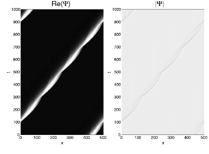
Figure 6: Space-time plots of ${\rm Re}(\Psi)$ and $|\Psi|$ for an oscillating kink. Same parameters as in Fig. 5a.

Figure 5b illustrates the kink replication process close to the transition to oscillating kinks. Initial condition was again the oscillatory unstable kink profile. $\Psi_{\rm min}(t)$ starts oscillating with increasing amplitude. At $t>1000$, the oscillation period increases significantly. At $t\approx 2500$, $\Psi_{\rm min}(t)$ breaks down to zero periodically, corresponding to the destruction of the kink and the subsequent creation of a new pair of counter-propagating kinks.

To get more information about the oscillatory instability, the eigenvectors belonging to the pair of unstable complex conjugated eigenvalues were computed. They form a pair of complex conjugated eigenvectors representing the complex amplitude of the oscillatory perturbation (for the linear stability analysis, the real and imaginary parts of the complex field $\Psi$ are treated as independent real variables, i.e., there are two complex perturbation fields acting on ${\rm Re}(\Psi)$ and ${\rm Im}(\Psi)$, respectively). In Fig. 7, spatial profiles of ${\rm Re}(\Psi)$ and the real part of the perturbation acting on ${\rm Re}(\Psi)$ are plotted for a spectrum shown in Fig. 4b. One can see an oscillatory perturbation with increasing amplitude on the tail of the kink. (As the kink is propagating at positive velocity, “tail” refers to the left part of the profile shown in the figure).

Figure 7: ${\rm Re}(\Psi)$ for an oscillatory unstable kink profile (solid line) and real part of the perturbation field acting on ${\rm Re}(\Psi)$ (dashed line). The perturbation field corresponds to the eigenvector belonging to the unstable pair of complex conjugated eigenvalues of the spectrum shown in Fig. 4b.

For further decreasing $\nu$, one can observe that the oscillation period $T_{\rm o}$ of the propagating kink profiles increases. At $\nu=\nu_{\rm kr}$, $T_{\rm o}$ diverges and the kink profile evolved from the oscillatory unstable profile remains for a long time close to the coexisting saddle profile. If $\nu<\nu_{\rm kr}$, the kink profiles are destroyed and the kink replication process begins. Figure 5b shows $|\Psi|_{\rm min}(t)$ in the kink replication regime close to the transition to oscillating kinks. If a kink is destroyed in a defect, $|\Psi|_{\rm min}(t)$ drops to zero. The periods of the kink oscillations $T_{\rm o}$ and the kink replication $T_{\rm kr}$ are plotted vs. $\nu$ in Fig. 8. The divergence of both $T_{\rm o}$ and $T_{\rm kr}$ at $\nu\approx\nu_{\rm kr}$ can be clearly seen.

Figure 8: Period of kink replication  $T_{\rm kr}$ (circles) and kink oscillation period $T_{\rm o}$ (stars) vs. $\nu$ at the transition oscillating kinks – kink replication (parameters: $\alpha=-0.75$, $\beta=1.8$, $B=0.015$).

The kink replication process leads to characteristic Sierpinski gasket-like spatiotemporal pattern which can be observed in a wide range of systems. The resulting dynamics can be seen as a form of STI Chaté et al. (1999). Close to the transition at $\nu=\nu_{\rm kr}$, a new form of STI involving oscillating kinks can be found. In the left panel of Fig. 9, a space-time plot of such STI is shown. The time series $|\Psi|_{\rm min}(t)$ in the right panel of Fig. 9 illustrates the oscillatory transients of a kink between two subsequent kink replication events.

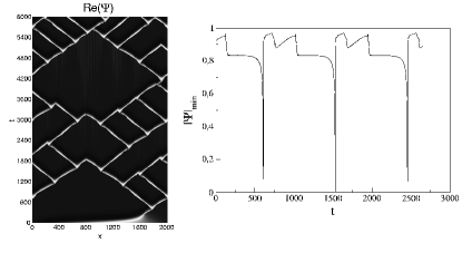
Figure 9: Kink replication involving oscillating kinks at $\alpha=-0.75$, $\beta=1.8$, $B=0.015$, $\nu=-0.765985$. Left: space-time plot of the real part of the complex oscillation amplitude ${\rm Re}(A)$. Right: $|\Psi|_{\rm min}(t)$ computed in a comoving reference frame as in Fig. 5.

Although the kink replication period $T_{\rm kr}$ obviously diverges, if $\nu$ approaches $\nu_{\rm kr}$, it was not possible to find a scaling law. The appearance of additional local maxima of $T_{\rm kr}(\nu)$ for $\nu<\nu_{\rm kr}$ in Fig. 8 indicates that the parameter dependence of $T_{\rm kr}$ is very complicated. Thus, simple scaling laws might fit only in small parameter intervals which cannot be resolved numerically.

The numerical results can be interpreted as follows: The transition from stable kinks to a hysteresis regime, where stable kinks and oscillating kinks coexist as attractors with decreasing $\nu$ is typical for a saddle-node bifurcation of limit cycles. Branches of stable and unstable limit cycles are created. The unstable limit cycle corresponds to a localized oscillatory propagating object that acts as a separatrix in the phase space. It separates spatial profiles that evolve to a stable kink from those evolving to an oscillating kink. Another indicator for a saddle-node bifurcation of limit cycles is the fact that the oscillations of the kink profile have a finite amplitude at their onset.

With decreasing detuning $\nu$, the stable kink profiles associated with the lower branch in the bifurcation diagram (Fig. 3) undergo a Hopf bifurcation. This Hopf bifurcation is subcritical: The unstable oscillatory kink profile merges with the stationary kink profile associated with that branch. As a consequence, they undergo an oscillatory instability leading to the coexistence of an oscillatory unstable kink profile and a stable limit cycle. If $\nu$ is further decreased, the stable limit cycle collides with the saddle kink profile corresponding to the upper branch in the bifurcation diagram (Fig. 3) and is destroyed in a homoclinic Andronov bifurcation. The divergence of the kink oscillation period is an indication for this type of bifurcation. Numerical simulations at $\nu\approx\nu_{\rm kr}$ reveal that the oscillating kink profiles remain for a long time close to the saddle profile corresponding to the upper branch in the bifurcation diagram (Fig. 3) . Consequently, the average velocity of the oscillating kink profiles converges to the velocity of the saddle kink profiles for $\nu\to\nu_{\rm kr}$ .

At $\nu>\nu_{\rm kr}$, no stable attractor associated to propagating kinks exists, and any kink-like object will be destroyed in a defect after a certain transient. In the above discussed case with $B=0.015$ this leads to kink replication.

III.2 Example 2: Transition stable kinks – no kinks

More complicated scenarios can be encountered at the transition stable kinks – oscillatory propagating kinks – no kinks for higher values of the forcing amplitude $B$. In Fig. 10, a bifurcation diagram for $B=0.022$ is presented, again with $\nu$ as the bifurcation parameter. As in the previously discussed case for $B=0.015$, the upper branch in the diagram corresponds to saddle unstable kink profiles, since the lower branch is associated to oscillatory unstable kink profiles resulting from a Hopf bifurcation of the stable profiles, which are indicated by a solid line. Oscillatory propagating kink profiles are again indicated by their average velocity. Starting decreasing $\nu$ in the stable kink regime at the right boundary of the diagram in Fig. 10, one first encounters a region with multistability for $-0.75515>\nu>-0.7573$ (IV in Fig. 10). In this parameter interval, two stable attractors coexist corresponding to stable and oscillating kinks. It is separated by an intermediate stable kink region (V in Fig. 10) from another multistable region at lower values of $\nu$. Therefore, oscillatory kinks in this multistable region can only be found by starting in an oscillatory kink region and varying both $B$ and $\nu$. At $\nu=-0.7591$, a branch of oscillating kink profiles appears, leading again to multistability and hysteresis between stable and oscillatory kinks (IV in Fig. 10). At $\nu=-0.75981$, the branch of stable kink profiles is turned into a branch of oscillatory unstable profiles in a Hopf bifurcation, and only oscillatory kinks are possible (III in Fig. 10). At $\nu_{0}=-7600868$, a transition oscillating kinks – no kinks takes place. However, in contrast to the situation at the transition to the kink replication regime, at $\nu_{1}=-0.7618857$, a new branch of oscillatory kink profiles appears. In this regime (II in Fig. 10), oscillatory kinks can be found only for certain initial conditions with a phase rotation of $2\pi$, whereas in the oscillatory kink regime at higher values of $\nu$ (III in Fig. 10) each such initial condition $2\pi$ seems to evolve to a kink profile. This bistable region disappears at $\nu_{2}=-0.7624856$ in another transition from oscillating kinks to a homogeneous state without kinks (I in Fig. 10).

Figure 10: Bifurcations of the kink profiles ($B=0.022$, other parameters as in Fig. 3). Dashed (dotted) lines denote branches of saddle (oscillatory unstable/unstable node) kink profiles. The Roman numerals denote the different dynamical regimes: (I) No kinks, (II) bistability no kinks – oscillating kinks, (III) oscillating kinks, (IV) multistability oscillating kinks – stable kinks.

Let us now have a closer look at the transitions to a spatially homogeneous state without kinks. If those transitions occur with decreasing $\nu$ (at $\nu=\nu_{0}$ and $\nu=\nu_{2}$), the kink oscillation period was found to increase, when the transition was approached.

To get a further insight into the nature of the transition, the oscillation period $T_{\rm osc}$ of the oscillating kinks was measured from the time series $|\Psi|_{\rm min}(t)$ for $\nu>\nu_{0}$ and $\nu>\nu_{2}$. The results are presented in the left panel of Fig. 11 as semi-log plots vs. distance to the transition $\nu-\nu_{0}$ and $\nu-\nu_{2}$, respectively. The oscillation period diverges in both cases as $T_{\rm osc}=1/\lambda\log(\nu-\nu_{0})$ [$T_{\rm osc}=1/\lambda\log(\nu-\nu_{2})$]. The right panel of Fig. 11 shows the result of the linear stability analysis performed for kink profiles belonging to the upper branch in the bifurcation diagram at $\nu=\nu_{0}$ and $\nu=\nu_{2}$, respectively. One can see one real eigenvalue beyond the imaginary axis indicating a saddle. The values of $\lambda$ obtained by fitting the logarithmic divergence law with the unstable eigenvalue of the linearized operator are in good agreement. This is again a clear indication of a homoclinic Andronov bifurcation involving the branch of saddle unstable kink profiles shown as dashed line in Fig. 10.

Figure 11: Upper panel Left: Semi-log plot of the kink oscillation period $T_{\rm osc}$ vs. distance to the transition $\nu-\nu_{0}$. Right: Eigenvalues of the linearized operator for $B=0.022$, $\nu=-0.7600868$, $V=1.07608$ (circle in Fig. 10). A positive real eigenvalue $\lambda=0.05373$ indicates a saddle.
Lower panel Left: Semi-log plot of the kink oscillation period $T_{\rm osc}$ vs. distance to the transition $\nu-\nu_{2}$. Right: Eigenvalues of the linearized operator for $B=0.022$, $\nu=-0.7624856$, $V=1.04418$ (square in Fig. 10).

At $\nu=\nu_{1}$, where the transition to a homogeneous state without kinks takes place, if $\nu$ is increased, no divergence of the kink oscillation period was found. However, at $\nu>\nu_{1}$, oscillating kink profiles exist as transients before being destroyed via the creation of a defect. The length of these transients increases when approaching the transition. This can be seen as an indicator for a saddle-node bifurcation of the oscillatory kink profiles. The appearance of intermediate regimes with oscillatory kinks might be connected to a complicated bifurcation scenario of limit cycles associated with propagating oscillating kinks, similar to that observed for stationary kink profiles.

IV A phase diagram

Studies of transitions to the regime with stable propagating kinks have been carried out for a wide range of parameters. A rough phase diagram showing the different regimes in the $B$-$\nu$ plane is given in Fig. 12.

Figure 12: Rough phase diagram in the $\nu$-$B$ plane. Left: Boundary of the region, where spatially homogeneous steady states exist (Arnold tongue, solid line), and stability boundary of the spatially homogeneous state (dotted line). Below the line, the spatially homogeneous state becomes linearly unstable. Right: Enlargement of the rectangular-shaped region in the left panel. The solid line denotes again the boundary of the Arnold tongue. Additionally, the lines, where the bifurcations discussed in the text take place, are shown.

The dashed line in Fig. 12 indicates homoclinic bifurcations at the transition no kinks – oscillating kinks and kink replication – oscillating kinks (the line corresponding to the transition between kink replication and no kinks is not shown). At higher values of $B$, several transitions no kinks – oscillating kinks are possible, when $\nu$ is varied. The dashed line in Fig. 12 always corresponds to the last appearance of oscillating kinks, when $\nu$ is decreased. This means that on the left side of the dashed line in Fig. 12 no oscillatory kinks are possible, whereas on the right side of this line oscillating kinks can be found except for some small parameter regions in the upper part of the diagram at higher values of $B$. The Hopf bifurcation of kink profiles is shown as dotted line. It separates the region with oscillatory kinks from the bistable region, where oscillatory and stable kinks coexist. The dashed-dotted line marks the saddle-node bifurcation of oscillatory kink profiles. It is the boundary between the bistable region and the regions, where only stable kinks exists. The appearance of intermediate regions with stable kinks or bistability again indicates complicated bifurcation scenarios of limit cycles corresponding to oscillatory kinks at higher values of $B$

The locations of the bifurcation lines in the parameter space show that the scenarios presented above are typical for transitions from stable kinks to kink replication or to no kink regimes, reflecting the tendency to more complicated transition scenarios at higher values of $B$.

V Conclusions

The transitions stable kinks – kink replication and stable kinks – no kinks studied in this work are connected to the synchronization of phase turbulence in the CGLE by external forcing.

It turned out that the parameter regions, where kink profiles exist, are not indentical to those with stable kinks. The boundaries of the latter are determined by instabilities of the kink profiles. This leads to intermediate regimes with new types of attractors such as limit cycles associated with oscillatory propagating kinks. Multistable regimes where stable kinks and oscillating kinks as attractors coexist are also possible. The destruction of those attractors is responsible for the transition either to kink replication or to a spatially homogeneous state. Instead of a single saddle-node bifurcation, the kink profiles undergo complicated bifurcation scenarios leading to the coexistence of several kink profiles. In those scenarios the creation of branches of stable kinks was also observed. As a consequence, transition scenarios with intermediate regimes of stable kinks are possible.

Moreover, at the transition from oscillatory kinks to a spatially homogeneous state without kinks intermediate regions with oscillatory kinks can be encountered. A possible explanation could be that their existence is due to a complicated bifurcation scenario of the limit cycles corresponding to oscillating propagating kinks involving saddle-node bifurcations of limit cycles. Another indication for this assumption is the appearance of an intermediate stable kink region in the phase diagram in Fig 12. In the present work, these saddle-node bifurcations of limit cycles were only observed in connection with transitions oscillating kinks – stable kinks or oscillating kinks – no kinks. However, if one varies the values of $\alpha$ and $\beta$, saddle-node bifurcations connected to transitions oscillating kinks – STI might be possible. Perhaps, such a transition could lead to new forms of STI.

The oscillating propagating phase kinks are the result of a new type of instability which is presumably favored at higher values of the dispersion coefficient $\beta$ of the CGLE. Numerical studies have been carried out revealing very complicated bifurcation scenarios of the kinks involving non-coherent structures like oscillating kinks. These scenarios are not yet completely understood. One can assume that they occur in a wide range of parameters. The present work can be a starting point for further systematical investigations.