Oscillating tails of dispersion-managed soliton

Abstract

Oscillating tails of dispersion-managed optical fiber system are studied for strong dispersion map in the framework of path-averaged Gabitov-Turitsyn equation. The small parameter of the analytical theory is the inverse time. An exponential decay in time of soliton tails envelope is consistent with nonlocal nonlinearity of Gabitov-Turitsyn equation, and the fast oscillations are described by a quadratic law. The pre-exponential modification factor is the linear function of time for zero average dispersion and cubic function for nonzero average dispersion.

I Introduction

A dispersion management is key current technology for development of ultrafast high-bit-rate optical communication lines kogelnik1 ; kurtzke1 ; chrapl1 ; smithknox1 ; gabtur1 ; gabtur2 ; kumar1 ; kaup1 ; mamyshev1 ; mamyshev2 ; turitsyn1 ; medvedev2002 ; gajadharsingh2004 . A dispersion-managed (DM) optical fiber is designed to achieve low (or even zero) path-averaged group velocity dispersion by periodic alternation of the sign of the dispersion along an optical line which dramatically reduces pulse broadening.

If nonlinearity is neglected it would be possible to achieve transmission of optical pulses through DM system without significant distortion. However, the linear transmission is limited by the nonlinear distance $z<z_{nl}\equiv(\sigma|u_{0}|^{2})^{-1}$, which is determined by the Kerr nonlinearity $\sigma$ and the characteristic pulse power $|u_{0}|^{2}$; $z$ is the propagation distance along fiber. The characteristic power can not be chosen too small in order to maintain appropriate value of the signal-to-noise ratio. As a result, Kerr nonlinearity is essential for pulse propagation which results in distortion of optical pulses and finite bit error rate (BER) for information transmission. There are two alternative approaches to deal with optical nonlinearity.

First approach is to reduce nonlinearity i.e. to make fiber system as close as possible to linear system. E.g. one can use low nonlinearity fiber Hamaide95 ; Weins97 with increased cross section. Another approach is to compensate nonlinearity (nonlinearity management) using either semiconductor devices  pare1996 or interferometer-based compensation of nonlinear phase shift GabitovLushnikov2002 . These systems usually refer to as quasi-linear systems and they attracted very much attention in recent years. Disadvantage of quasi-linear systems is that nonlinearity is still essential at long enough distancemamyshev1 ; mamyshev2 (e.g. transoceanic distance) and it results in information losses. Also quasi-linear systems often require complex and cumbersome dispersion compensationmollenauer1tb2003 .

Second approach is not to reduce nonlinearity but rather to use nonlineariy to achieve high bit rate transmission. This approach is based on a concept of using of DM solitons as the carrier of a bit of information. DM soliton is a solitary pulse which propagates in optical fiber smithknox1 ; gabtur1 ; gabtur2 ; kumar1 ; kaup1 ; mamyshev1 ; mamyshev2 ; turitsyn1 . DM soliton experiences periodic oscillations, as a function of propagation distance, with period of dispersion compensation. Single DM soliton can propagate in optical fiber without distortion (except periodic oscillations) for arbitrary long distance even for nonzero path-averaged dispersion (dispersion, averaged over period of dispersion variation). Propagation without distortion results from balance between nonlinearity and dispersion on the period of dispersion compensation. In contrast, quasi-linear pulse would increase its width with propagation distance (in addition to periodic oscillations) due to nonzero path-averaged dispersion.

DM soliton-based transmission has its own disadvantages caused by interaction between different DM solitons (representing different bits of information). There are two types of interactions. First type is caused by the interaction between DM solitons with the same carrier frequency (the same information channel). In addition, modern optical lines use a wavelength-division multiplexing (WDM) which allows the simultaneous transmission of several information channels, modulated at different wavelengths, through the same optical fiber. WDM means that there is also a second type of interaction, which is the interaction between DM solitons in different channels. Traditionally, the second type is considered to be the most dangerous because DM solitons in different channels move with different group velocity and, respectively, they pass through each other causing collisions through nonlinear interaction. Collisions result in a jitter in DM soliton arrival times and finite BER. However, recently, the record-breaking, 1.09Tbits/s, transmission was achieved at 18,000 km optical line based on DM solitons mollenauer1tb2003 which brought increasing interest to DM soliton-based transmission systems. The interchannel interactions in that transmission experiment were suppressed by a periodic-group-delay dispersion-compensating module mollenauerdelay2003 , and intrachannel interaction is most important. The main purpose of this Article is to determine the tails DM soliton which determines the interaction of DM solitons in the same channel. Soliton tails are responsible for interaction of pulses launched into optical fiber which essentially limits bit-rate capacity of optical line and makes finding DM soliton asymptotic behaviour an important practical and fundamental problem. It is found that envelope of soliton decays exponentially in time (much slower decay compare to Gaussian) so one can expect a strong interaction of different DM solitons.

II Path-averaged equation

Neglecting polarization effects, higher order dispersion, losses, stimulated Raman scattering and Brillouin scattering, the propagation of optical pulse in a DM fiber is described by a scalar nonlinear Schrödinger equation (NLS)

$$iA_{Z}-\frac{1}{2}\beta_{2}(Z)A_{TT}+\sigma(Z)|A|^{2}A=0,$$ (1)

where $A$ is the envelope of optical pulse, $Z$ is the propagation distance, $T$ is the retarded time, $\beta_{2}(Z)$ is the group-velocity dispersion which is the periodical function of $Z$, $\sigma(Z)=(2\pi n_{2})/\big{(}\lambda_{0}A_{eff}(z)\big{)}$ is the nonlinear coefficient, $n_{2}$ is the nonlinear refractive index, $\lambda_{0}=1.55\,\mu m$ is the carrier wavelength, $A_{eff}$ is the effective fiber area that in general case depends on $Z$. Typical values of dispersion and nonlinear coefficient are $\beta_{2}=-20.0\,\mbox{ps}^{2}/\mbox{km},$ $\sigma=0.0013\,(\mbox{km}\,\mbox{mW})^{-1}$ for standard monomode fiber, and typical values for dispersion compensating fiber are $\beta_{2}=103.9\,\mbox{ps}^{2}/\mbox{km},$ $\sigma=0.00405\,(\mbox{km}\,\mbox{mW})^{-1}$.

It is convenient to introduce the dimensionless variables: $z=Z/l_{0},\ t=T/t_{0},\ u=A/\sqrt{P_{0}}$, where $l_{0}$ is the typical period of dispersion variation, $t_{0}$ is the typical pulse duration and $P_{0}$ is the typical pulse power. For typical optical lines $l_{0}\sim 50\,\mbox{km}$,  $t_{0}\sim 10\mbox{ps},\ P_{0}\sim 1\,\mbox{mW}$. Eq. $(\ref{nls1})$ in dimensionless variables takes the following form:

$$iu_{z}+d(z)u_{tt}+c(z)|u|^{2}u=0,$$ (2)

where $c(z)=\sigma(z)P_{0}l_{0},\ d(z)=-\beta_{2}l_{0}/(2t_{0}^{2})$. Consider a two-step periodic dispersion map (see Fig. 1): $d(z)=\langle d\rangle+\tilde{d}(z)$, where $\tilde{d}(z)=d_{1}$ for $0<z+nL<L_{1}$ and $\tilde{d}(z)=d_{2}$ for $L_{1}<z+nL<L$, $L\equiv L_{1}+L_{2}$ is the dispersion map period, $\langle d\rangle$ is the path-averaged dispersion, $d_{1},d_{2}$ are the amplitudes of dispersion variation subjected to condition $d_{1}L_{1}+d_{2}L_{2}\equiv 0$ and $n$ is an arbitrary integer number. Path averaged dispersion is assumed to be small, $|\langle d\rangle|\ll|d_{1}|,\,|d_{2}|.$

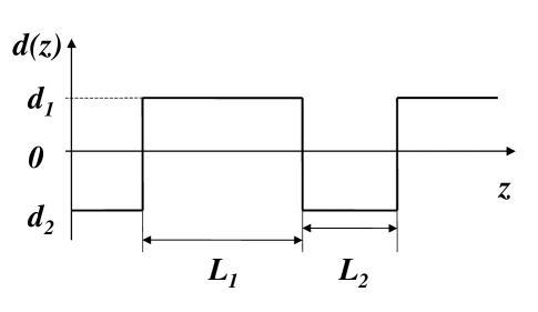
Figure 1: Dispersion $d(z)$ as function of propagation distance $z$.

Optical pulse experiences strong oscillation as a function of $z$ on the period of dispersion map $L$. These oscillations are caused primarily by linear effects which are described by the linear part of Eq. $(\ref{nls1})$.

A typical power of pulse is about a few $mW$ in most optical fiber systems. As a result the nonlinearity in Eq. $(\ref{nls1})$ can be treated as a small perturbation on scales of typical dispersion map period $L\sim 50km$ because the characteristic nonlinear length $Z_{nl}$ of the pulse is large: $Z_{nl}\gg L,$ where $Z_{nl}=1/|p|^{2}$ and $p$ is the typical pulse amplitude. As nonlinearity is small perturbation on distance $L$, it is convenient to introduce the new variable$\psi:$ $\hat{\psi}\equiv\hat{u}e^{i\omega^{2}\int^{z}_{L_{1}/2}\tilde{d}(z^{\prime})dz^{\prime}}$. Here $\hat{\psi}(\omega)=\int^{\infty}_{-\infty}\psi(t)e^{\imath\omega t}dt$ is Fourier transform of $\psi$ and similar to $\hat{u}$. $\psi$ is the slow function of $z$ on the scale $L$ because all fast linear dependence on $z$ is included into fast varying exponent $e^{-i\omega^{2}\int^{z}_{L_{1}/2}\tilde{d}(z^{\prime})dz^{\prime}}$.

Fourier transform of Eq. $(\ref{nls1})$ gives:

$$i\hat{\psi}_{z}(\omega)-\omega^{2}\langle d\rangle\hat{\psi}+\frac{c(z)}{(2\pi)^{2}}\int\exp\Big{[}-i\triangle\int^{z}_{L_{1}/2}\tilde{d}(z^{\prime})dz^{\prime}\Big{]}$$

$$\times\hat{\psi}(\omega_{1})\hat{\psi}(\omega_{2})\hat{\psi}^{*}(\omega_{3})\delta(\omega_{1}+\omega_{2}-\omega_{3}-\omega)d\omega_{1}d\omega_{2}d\omega_{3},$$ (3)

where $\triangle\equiv\omega_{1}^{2}+\omega_{2}^{2}-\omega_{3}^{2}-\omega^{2}$. Because $\hat{\psi}$ is the slow function one can approximate its derivative as $\hat{\psi}(z)_{z}\simeq[\hat{\psi}(z+L)-\hat{\psi}(z)]/L$ and integrate Eq. $(\ref{psiint0})$ over dispersion map period $L$ neglecting the dependence of $\psi$ on $z$ in the nonlinear term. This averaging procedure results in path-averaged Gabitov-Turitsyn gabtur1 ; gabtur2 model:

$$i\hat{\psi}_{z}(\omega)-\omega^{2}\langle d\rangle\hat{\psi}+\frac{c_{0}}{(2\pi)^{2}}\int\frac{\sin{\frac{s\triangle}{2}}}{\frac{s\triangle}{2}}\hat{\psi}(\omega_{1})\hat{\psi}(\omega_{2})$$

$$\times\hat{\psi}^{*}(\omega_{3})\delta(\omega_{1}+\omega_{2}-\omega_{3}-\omega)d\omega_{1}d\omega_{2}d\omega_{3},$$

$$c_{0}=(c_{1}L_{1}+c_{2}L_{2})/L,$$ (4)

where $s=d_{1}L_{1}$ is the dispersion map strength, and $c_{1},\ c_{2}$ are the values of $c(z)$ for $0<z+nL<L_{1}$ and $L_{1}<z+nL<L$, respectively. It is set below, without loss of generality, that $c_{0}=1$ because one can always define typical power $P_{0}$ in such a way to insure $c_{0}=1.$ Note that Gaitov-Turitsyn Eq. can be also obtained by averaging of the Hamiltonian, $H=\int\big{[}d(z)|\psi_{t}|^{2}-|\psi|^{4}/2\big{]}dx$, of NLS $(\ref{nls1})$ over dispersion map period gabtur2 . The numerical solutions of the Gabitov-Turitsyn model were compared with simulations of full NLS $(\ref{nls1})$ which showed good agreement turitsyn1 ; ablowitz1 . Returning to time domain in Eq. $(\ref{psiint1})$ one gets ablowitz1 :

$$i\psi_{z}+\langle d\rangle\psi_{tt}-\frac{1}{2\pi s}\int Ci(\frac{t_{1}t_{2}}{s})\psi(t_{1}+t)\psi(t_{2}+t)\times$$

$$\psi^{*}(t_{1}+t_{2}+t)dt_{1}dt_{2}=0,$$ (5)

where $Ci(x)=\int^{x}_{\infty}\frac{\cos{x}}{x}dx$ (note difference in definition of $Ci(x)$ in comparison with ablowitz1 ).

Equation for DM soliton solution, $\psi=A(t)e^{i\lambda z}$ ($A$ is real), of the Gabitov-Turitsyn Eq. $(\ref{psiint1b})$ takes the following form:

$$-\lambda A+\langle d\rangle A_{tt}=\frac{1}{2\pi s}\int r(t_{1},t_{2},t)dt_{1}dt_{2},$$

$$r(t_{1},t_{2},t)=Ci\big{(}\frac{t_{1}t_{2}}{s}\big{)}A(t_{1}+t)A(t_{2}+t)A(t_{1}+t_{2}+t),$$ (6)

where $Ci(x)=\int^{x}_{\infty}\cos{x}/xdx$.

Eq. $(\ref{psiint1c})$ is used throughout this Article Eq. to study DM soliton.

III DM soliton tails

The previous studies kurtzke1 ; chrapl1 ; smithknox1 ; gabtur1 ; gabtur2 ; kumar1 ; kaup1 ; turitsyn1 ; pelin2000 ; zharnitsky1 ; zharnitsky2 ; Kunze2003 ; lush2000a ; lush2000b ; lush2001a have essentially focused on finding of DM soliton width, amplitude and soliton shape near soliton center. It was found that Gaussian ansatz,

$$A_{Gauss}=p\exp{\big{(}-\frac{\beta}{2}t^{2}\big{)}},$$ (7)

where $p,\beta$ are real constants, is a rather good approximation for the DM soliton solution near soliton center smithknox1 . Solution of Eq. $(\ref{psiint1c})$ by iterations allows to find soliton amplitude and width analytically with accuracy $\sim 1\%$ (see Refs. lush2000a ; lush2001a ). Note that parameters $s,\,\langle d\rangle,\,\lambda$ uniquely determine the numerical form of DM soliton lush2001a . E.g. for $\langle d\rangle=0$, $\beta s=2.393\ldots,\ \lambda=p^{2}\times 0.482\ldots$ lush2000a . Thus dispersion map strangth, $\beta s$, is fixed and not small for DM soliton. However an important question about asymptotic behavior of soliton tail for large time $t$ was only marginally addresses in the past pelin2000 ; lush2001a . Soliton tails are responsible for interaction of pulses launched into optical fiber which essentially limits bit-rate capacity of optical line and makes finding DM soliton asymptotic behaviour an important practical and fundamental problem. DM soliton tails behaviour is the main subject of this Article.

Solid curves in Fig. 2a and Fig. 2b show

(a)

(b)

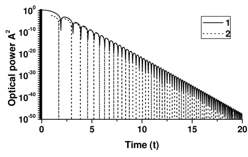
Figure 2: DM soliton shape (curve 1) versus Eq. (4) (curve 2) for (a) $\langle d\rangle=0,\ s=1,\ \lambda=1.$ and (b) for $\langle d\rangle=0.1,\ s=1,\ \lambda=1.$ $A(t)$ is an even function.

high precision numerical solution of Eq. $(\ref{psiint1c})$ for zero (Fig. 2a) and nonzero (Fig. 2b) values of averaged dispersion. Numerical technique for solving Eq. $(\ref{psiint1c})$ was developed in Refs. lush2001a ; lush2002a . Analysis of numerical solutions in Fig. 2 allows to make hypothesis that at leading order the asymptotic behaviour of $A$ is given by

$$A_{asymp}(t)=f(t)\cos\{t^{2}[a_{0}+a(t)]\}\exp(-b|t|),$$ (8)

where $a_{0},\,b$ are constants and $f(t),\,a(t)$ are slow functions of $t$. First it will be shown that an ansatz $(\ref{psishort0})$ is consistent with Eq. $(\ref{psiint1c})$ at leading order of $1/|t|$ provided $a_{0}=1/2s$ for $f(t)=const,\,a(t)=const$ and later it will be found an expansion of $f(t),\,a(t)$ over small parameter $1/|t|$. That result was announced without derivation in Ref. lush2001a for particular case $\langle d\rangle=0$. Here general case which includes both $\langle d\rangle=0$ and $\langle d\rangle\neq 0$ is considered.

First necessary condition for consistency of the ansatz $(\ref{psishort0})$ with Eq. $(\ref{psiint1c})$ is that a substitution of the envelope of soliton solution tails, $A_{env}\sim\exp{(-b|t|)}$, into right hand side (r.h.s.) of Eq. $(\ref{psiint1c})$ should recover the same exponential dependence on $t$ after integration over $t_{1},t_{2}$ variables in Eq. $(\ref{psiint1c})$. Asymptotic behaviour for $|x|\to\infty$ of kernel in r.h.s. of Eq. $(\ref{psiint1c})$ is given by:

$$Ci(x)=sin(x)/x+O(1/x^{2})$$ (9)

and $Ci(t_{1}t_{2}/s)$ produces at leading order the contribution to phase of $A(t)$ only but not to envelope $A_{env}$. The contribution of other factors in $r(t,t_{1},t_{2})$ to $A_{env}$ is given by

$$A(t_{1}+t)A(t_{2}+t)A(t_{1}+t_{2}+t)$$

$$\simeq\exp\Big{(}-b[|t_{1}+t|+|t_{2}+t|+|t_{1}+t_{2}+t|]\Big{)}$$ (10)

and decays much faster than $e^{-b|t|}$ outside the triangle ABC (shown in Fig. 3 for $t>0$).

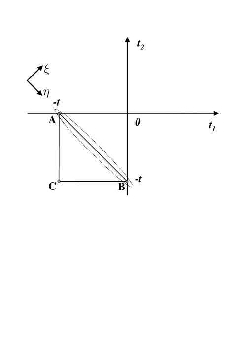
Figure 3: Integration plane $(t_{1},t_{2})$ for Eq. (3). $t>0.$ Characteristic layer is located along AB inside the dotted curve. lushnikovfig3.eps

Triangle ABC is defined in $(t_{1},t_{2})$ plane and determined from condition $t_{1}+t>0,\ t_{2}+t>0,\ t_{1}+t_{2}+t<0$. However, inside the triangle $A(t_{1}+t)A(t_{2}+t)A(t_{1}+t_{2}+t)\simeq e^{-b|t|}$, which recovers the exponential decay as it appears at left hand side (l.h.s.) of Eq. $(\ref{psiint1c})$. One can conclude that $A_{env}\sim e^{-b|t|}$ is compatible with Eq. $(\ref{psiint1c})$ and integration in plane $(t_{1},t_{2})$ inside an area outlined by dashed curve in Fig. 3 gives leading order contribution to r.h.s. of Eq. $(\ref{psiint1c})$ for $|t|\to\infty$. The area inside the dashed curve includes triangle $ABC$ and characteristic layers of the width $O(t^{0})$ which surround that triangle. Integration over the area outside of dashed curve in Fig. 3 gives exponentially small contribution of r.h.s. of Eq. $(\ref{psiint1c})$. E.g. $A(t_{1}+t)A(t_{2}+t)A(t_{1}+t_{2}+t)\simeq e^{-5b|t|}$ for $t_{1}\sim t/2,\ t_{2}\sim t/2$. This result is immediately confirmed by numerical calculation of integral in r.h.s of Eq. $(\ref{psiint1c})$ over the area inside the dashed curve for DM soliton solution and comparing result of integration with numerical integral over the whole $(t_{1},t_{2})$ plane. Numerical integration was performed using numerical procedure of Ref. lush2001a . Note the important fact that exponential envelope, $A_{env}$, is compatible with Eq. $(\ref{psiint1c})$ for any positive value of $b$ so that specific value of $b$, corresponding to DM soliton can be only obtained from more detail analysis of Eq. $(\ref{psiint1c})$.

Second necessary condition is that the substitution of fast oscillating function $A_{osc}\sim\cos{(t^{2}[a_{0}+a(t)])}$ into r.h.s. of Eq. $(\ref{psiint1c})$ should allow to reproduce the same oscillations as in l.h.s. of Eq. $(\ref{psiint1c})$ for $|t|\to\infty.$ Oscillating part of integrand $r(t,t_{1},t_{2})$ of r.h.s. of Eq. $(\ref{psiint1c})$ consists of product of one $sin$ function (from asymptotic of oscillating kernel $(\ref{ciasymp})$) and three $cos$ functions. Representing $sin$ and $cos$ through imaginary exponents one get a sum of 16 terms with different values of argument. 14 of them are always oscillate as a quadratic function of $t_{1},\,t_{2}$ and thus give vanishing contribution after integration over $t_{1},\,t_{2}$. Rest two terms can be made nonoscillating by appropriate choice of $a_{0}$. Thus integrand $r(t,t_{1},t_{2})$ of r.h.s. of Eq. $(\ref{psiint1c})$ at leading order, neglecting $a(t)$ inside the triangle ABC, can be represented as $r(t,t_{1},t_{2})\sim\exp\Big{(}it_{1}t_{2}/s+ia_{0}[(t_{1}+t)^{2}+(t_{2}+t)^{2}-(t_{1}+t_{2}+t)^{2}]-b|t|\Big{)}-c.c.+f.o.=\exp(it_{1}t_{2}/s-2ia_{0}t_{1}t_{2}+ia_{0}t^{2}-b|t|)-c.c.+f.o.$, where c.c. mean complex conjugation and f.o. designates 14 fast oscillating terms. Oscillations (as a quadratic function of $t_{1},\,t_{2}$) of argument of two rest terms vanish identically provided

$$a_{0}=1/(2s),$$ (11)

which is in excellent agreement with numerical solution of DM soliton $(\ref{psiint1c})$. Next step is to take into account nonzero value of $a(t)$ in Eq. $(\ref{psishort0})$. One can series expand

$$a(t)=a_{1}/|t|+a_{2}/t^{2}+O(1/|t|^{3})$$ (12)

and find that term $a_{1}|t|$ in argument of $cos$ of Eq. $(\ref{psishort0})$ causes oscillations of $r(t,t_{1},t_{2})$ as a linear function of $t_{1},t_{2}$. It is impossible to get rid of these oscillations for any value of $a_{1}$ so one can conclude that contribution of integration of $r(t,t_{1},t_{2})$ inside the triangle ABC vanishes meaning that leading order contribution to r.h.s of Eq.$(\ref{psiint1c})$ can only come from characteristic layers of the width $O(t^{0})$ which surround faces AB, BC and AC of triangle ABC. In the neighborhood of each of these faces either $t_{1}+t$ (face AC) or $t_{2}+t$ (face BC) or $t_{1}+t_{2}+t$ (face AB) is $\sim t^{0}$ so asympotic expression $(\ref{psishort0})$ is not valid but rather exact solution of Eq. $(\ref{psiint1c})$ should be used for respective factors $A(t_{1}+t)$, $A(t_{2}+t)$ or $A(t_{1}+t_{2}+t)$ in $r(t,t_{1},t_{2})$. Still there are fast oscillations of $r(t,t_{1},t_{2})$ as a function of $t_{1},t_{2}$ for integration inside the characteristic layers in directions parallel to faces BC and AC: $A(t_{1}+t)A(t_{1}+t_{2}+t)\sim e^{ia_{1}[2t+2t_{1}+t_{2}]-b|t_{2}|}+c.c.+f.o.$ (along BC) and $A(t_{2}+t)A(t_{1}+t_{2}+t)\sim e^{ia_{1}[2t+2t_{1}+t_{2}]-b|t_{1}|}+c.c.+f.o.$ (along AC). Thus integrations in these 2 layers give a vanishing contribution and only an integration in characteristic layer in the neighborhood of face AB gives leading order contribution. To check that result the numerical integration of integrand $r(t,t_{1},t_{2})$ with super Gaussian modification factor: $\tilde{r}(t,t_{1},t_{2})\equiv r(t,t_{1},t_{2})e^{-(|t+t_{1}+t_{2}|/t_{0})^{(2n)}}$, $n\gg 1$, $1\ll t_{0}\ll t$ was performed and it was found that $\int\tilde{r}(t,t_{1},t_{2})dt_{d}t_{2}=\int r(t,t_{1},t_{2})dt_{d}t_{2}+O(1/|t|)$ which confirms that only integration inside the characteristic layer around AB (that layer is schematically shown in Fig. 3 as the area inside the dashed curve) gives leading order contribution.

Analysis of an integration inside the characteristic layer AB is convenient to be performed in new variables:

$$\xi=t+t_{1}+t_{2},$$ (13)

$$\eta=t_{1}-t_{2},$$ (14)

where axes $\xi$ and $\eta$ are perpendicular and parallel to face AB, respectively (see Fig. 3). Face AB is located exactly at axis $\xi=0$. Keeping in mind that the width of characteristic layer is $\sim t^{0}\sim\xi$ while its length is $\sqrt{2}|t|\sim\eta$ one gets that the ratio of typical values of $\xi$ and $\eta$ is $\sim 1/|t|$ and $t_{1}+t=\frac{t+\eta}{2}+O(t^{0}),\ t_{2}+t=\frac{t-\eta}{2}+O(t^{0}),\ t_{1}=-\frac{t-\eta}{2}+O(t^{0}),\ t_{2}=-\frac{t+\eta}{2}+O(t^{0}).$ So that Eq. $(\ref{psiint1c})$, using Eq. $(\ref{ciasymp})$, is reduced at leading order of $1/|t|$ to

$$\Big{[}\lambda g(\langle d\rangle)+\langle d\rangle t^{2}/s^{2}\Big{]}f(t)\cos{\big{(}\frac{t^{2}}{2s}+a_{1}|t|+a_{2}\big{)}}$$

$$\times\exp{(-b|t|)}=\int\frac{d\xi}{4\pi}\int\limits^{t}_{0}d\eta\frac{A(\xi)f(\frac{t-\eta}{2})f(\frac{t+\eta}{2})}{(\eta-t)(\eta+t)}$$ (15)

$$\times\sin{\Big{(}[\xi^{2}+t^{2}]/2s+a_{1}[\xi+|t|]+2a_{2}\Big{)}}\exp{(-b\xi-b|t|)},$$

where the function $g(x)$ is used, $g(0)=1$ and $g(x)=1$ for $x\neq 0$, because term with $\lambda$ in l.h.s. of Eq. $(\ref{gtred2})$ is of leading order only if $\langle d\rangle=0$. There is a separation of the integration variables $\xi,\eta$ in r.h.s of Eq. and one can perform integration over $\xi$ to get reduced equation:

$$\Big{[}\lambda g(\langle d\rangle)+\langle d\rangle t^{2}/s^{2}\Big{]}f(t)=C_{1}\int\limits^{t}_{0}d\tilde{\eta}\frac{f(t-\tilde{\eta})f(\tilde{\eta})}{(t-\tilde{\eta})\tilde{\eta}},$$ (16)

where $\tilde{\eta}=\frac{t+\eta}{2}$; it is assumed without loss of generality that $t>0$; the real constant $C_{1}$ is given by

$$C_{1}=\int\frac{d\xi}{8\pi i}A(\xi)\exp{\Big{[}i(\xi^{2}/2s+a_{1}\xi+a_{2})-b\xi\Big{]}},$$

$$C_{1}=Re(C_{1}),$$ (17)

and $C_{1}=Re(C_{1})$ is the compatibility condition for Eq. $(\ref{gtred2})$ meaning that phase of $cos$ in both r.h.s. and l.h.s. (after integration over $\xi$) is the same and equals to $a_{2}$ for $|t|=0$. It is important that exact (not asymptotic) expression for $A(t)$ should be used in evaluating integral in Eq. $(\ref{C1})$ which means that asymptotic tails $(\ref{psishort0})$ are determined by strongly nonlocal effects because all time scales contribute to $C_{1}$.

The integral term in Eq. $(\ref{gtred3})$ is the convolution integral and using Laplace transform, $\tilde{f}_{p}\equiv\int^{\infty}_{0}dt\tilde{f}(t)e^{-pt}$, for function $\tilde{f}(t)=f(t)/t$ one gets an ordinary differential equation:

$$\lambda g(\langle d\rangle)\frac{d\tilde{f}_{p}}{dp}+\langle d\rangle\frac{1}{s^{2}}\frac{d^{3}\tilde{f}_{p}}{dp^{3}}=-C_{1}\tilde{f}_{p}^{2},$$ (18)

which has the following solution: $\tilde{f}_{p}=g(\langle d\rangle)\frac{\lambda}{C_{1}(p+C_{2})}+60\frac{\langle d\rangle}{C_{1}(p+C_{2})^{3}}$, where $C_{2}$ is an arbitrary real constant. Inversion of Laplace transform results in: $f(t)=\Big{[}tg(\langle d\rangle)\lambda+30t^{3}\langle d\rangle\Big{]}e^{-C_{2}t}/C_{1}$. For arbitrary sign of $t$ one should replace $t$ by $|t|$ in this expression. Factor $e^{-C_{2}|t|}$ gives renormalization of constant $b$ in Eq. $(\ref{psishort0})$, which reflects a freedom of choice of $b$ in Eq. $(\ref{psishort0})$ so $C_{2}$ could be set, without loss of generality, to zero and expression for $f(t)$ takes the following final form:

$$f(t)=\frac{\lambda|t|}{C_{1}}\ \ \mbox{for}\ \ \langle d\rangle=0,\quad f(t)=\frac{30\lambda|t|^{3}}{C_{1}}\ \ \mbox{for}\ \ \langle d\rangle\neq 0.$$ (19)

Eqs. $(\ref{at}),(\ref{fres1})$ have four real constants $C_{1},\,b,\,a_{1}$ and $a_{2}$ which can not be determined from leading order expansion developed in this Article because all time scales contribute to numerical values of these constants. One can easily find constants $C_{1},\,b,\,a_{1},\,a_{2}$ from a fit with numerical solution of Eq. $(\ref{psiint1c})$. Phase of $cos$ in Eq. $(\ref{psishort0})$ is determined from zeros of the numerical solution of $A(t)$ keeping in mind that coefficient $a_{0}=1/2s$ is known analytically. After the constants $a_{1},\,a_{2}$ are found, one can determine $C_{1}$ and $b$ numerically from a two-parameter fit with envelope of DM soliton tail oscillations. Fig. 2a,b show a good agreement between the numerical solution (curve 1) and $A_{asymp}(t)^{2}$ dependence (curve 2). Fig. 2a corresponds to $s=1,\lambda=1,\langle d\rangle=0$ and numerical values $C_{1}=0.08357,\,b=3.0452,\,a_{1}=1.4136,\,a_{2}=1.5102$. Fig. 2b corresponds to $s=1,\lambda=1,\langle d\rangle=0.1$ and numerical values $C_{1}=13.818,\,b=3.2483,\,a_{1}=0.1443,\,a_{2}=-0.1276$. $C_{1},\,b,\,a_{1},\,a_{2}$ are obtained from the above described fitting procedure. A similar plot for zero average dispersion $\langle d\rangle=0$ was given in Ref. lush2001a in Fig. 3. Note however that curve 2 in Fig. 2b converges to curve 1 for larger $t$ compare to the case $\langle d\rangle=0$ in Fig. 2a which reflects the fact that for intermediate values of time, $t\sim t_{i}$, $\langle d\rangle t_{i}^{2}=\lambda$, there is a transition from the solution of $f(t)$ in Eq. $(\ref{fres1})$ for $\langle d\rangle=0$ to the solution for $\langle d\rangle\neq 0.$ If $\langle d\rangle$ is large enough so that $t_{i}$ $\sim$ DM soliton width, then there is a transition from oscillating tails of DM soliton to nonoscillating exponential tails of NLS with constant dispersion $\langle d\rangle$. NLS soliton width, $(\lambda/\langle d\rangle)^{1/2},$ is much larger than DM soliton width for small $\langle d\rangle$.

IV Conclusion

In summary, the asymptotic, $|t|\to\infty$, of DM soliton tails is given by Eqs. $(\ref{psishort0}),(\ref{a0}),(\ref{at}),(\ref{fres1})$ which is in agreement with numerical solution of Eq. $(\ref{psiint1c})$. The pre-exponential factor (19) is qualitatively different for zero and nonzero path-averaged dispersion. An exponential decay of DM soliton envelope, which is much slower compare to Gaussian-type decay near soliton center, suggests that interaction of different DM solitons is strong and could affect bit-rate capacity of optical lines. A detailed investigation interaction between DM solitons is outside the scope of this Article. Another possible direction of future research is to study the effect of losses on DM soliton tails as well as DM soliton with nonlinearity compensation GabitovLushnikov2002 . Qualitatively oscillations are still of the form $(\ref{psishort0})$ but further research is needed.

The author thanks M. Chertkov, I.R. Gabitov, E.A. Kuznetsov, V.E. Zakharov and V. Zharnitsky for helpful discussions. The support was provided by the Department of Energy, under contract W-7405-ENG-36. The author’s E-mail address is lushnikov@cnls.lanl.gov.

References

- (1) C. Lin, H. Kogelnik and L.G. Cohen, “Optical-pulse equalization of low-dispersion transmission in single-mode fibers in the m spectral region”, Opt. Lett., 5, 476-478 (1980).
- (2) C. Kurtzke, “Suppression of fiber nonlinearities by appropriate dispersion management”, IEEE Phot. Tech. Lett., 5, 1250-1253 (1993).
- (3) A.R. Chraplyvy, A.H. Gnauck, R.W. Tkach and R.M. Derosier, “ Gb/s transmission through 280 km of dispersion-managed fiber”, IEEE Phot. Tech. Lett., 5, 1233-1235 (1993).
- (4) N.J. Smith, F.M.Knox, N.J. Doran, K.J. Blow and I. Bennion, “Enhanced power solitons in optical fiber transmission line”, Electron. Lett., 32, 54-55 (1996).
- (5) I. Gabitov and S.K. Turitsyn , “Averaged pulse dynamics in a cascaded transmission system with passive dispersion compensation”, Opt. Lett., 21, 327-329 (1996).
- (6) I. Gabitov and S.K. Turitsyn , “Breathing solitons in optical fiber links”, JETP Lett., 63, 861-866 (1996).
- (7) S. Kumar and A. Hasegawa, “Quasi-soliton propagation in dispersion-managed optical fibers”, Opt. Lett., 22, 372-374 (1997).
- (8) T. Lakoba and D.J. Kaup, “Shape of the stationary pulse in the strong dispersion management regime”, Electron. Lett. 34, 1124-1125 (1998).
- (9) P.V. Mamyshev and N.A. Mamysheva., “Pulse-overlapped dispersion-managed data transmission and intrachannel four-wave mixing”, Opt. Lett., 24, 1454-1456 (1999).
- (10) L.F. Mollenauer, P.V. Mamyshev, J. Gripp, M.J. Neubelt, N. Mamysheva, L. Grüner-Nielsen and T. Veng, “Demonstration of massive wavelength-division multiplexing over transoceanic distances by use of dispersion-managed solitons”, Opt. Lett., 25, 704-706 (1999).
- (11) S.K. Turitsyn, T. Schäfer, N.J. Doran, K.H. Spatschek and V.K. Mezentsev, “Path-averaged chirped optical soliton in dispersion-managed fiber communication lines”, Opt. Comm. 163, 122-158 (1999).
- (12) S.B. Medvedev, O.V. Shtyrina, S.L. Musher, and M.P. Fedoruk, “Path-averaged optical soliton in double-periodic dispersion-managed systems”, Phys. Rev. E, 66, 066607 (2002).
- (13) A. Gajadharsingh, and P.-A. Bélanger, “Dispersion-managed solitons as the interference of chirped complex conjugate pulses”, Proc. of NLGW’2004, MC7.
- (14) J.P. Hamaide, F. Pitel, P. Nouchi, B. Biotteau, J. Von Wirth, P. Sansonetti, J. Chesnoy, “Experimental 10 Gb/s sliding filter-guided soliton transmission up to 19 Mm with 63 km amplifier spacing using large effective-area fiber management”, ECOC’95, 17-21 Sept. 1995, Brussels, Belgium.
- (15) C. Weinstein, “ Fiber design improves long-haul performance”, Laser Focus World, 33, 215 (1997).
- (16) C. Paré, A. Villeneuve, P.-A. Bélanger and N.J. Doran, “ Compensating for dispersion and the nonlinear Kerr effect without phase conjugation”, Opt. Lett., 21, 459-461 (1996).
- (17) I.R. Gabitov, and P.M. Lushnikov, “Nonlinearity management in dispersion managed system”, Opt. Lett. 27, 113-115 (2002).
- (18) L.F. Mollenauer, A. Grant, X. Liu, X. Wei, C. Xie, I. Kang, “Experimental test of dense wavelength-division multiplexing using novel, periodic-group-delay-complemented dispersion compensation and dispersion-managed solitons”, Opt. Lett., 28, 2043-2045 (2003).
- (19) X. Wei, X. Liu, C. Xie, L.F. Mollenauer, “Reduction of collision-induced timing jitter in dense wavelength-division multiplexing by the use of periodic-group-delay dispersion compensators”, Opt. Lett., 28, 983-985 (2003).
- (20) M.J. Ablowitz and G. Biondini, “Multiscale pulse dynamics in communication systems with strong dispersion management”, Opt. Lett., 23, 1668-1670 (1998).
- (21) P.M. Lushnikov, “ Dispersion-managed soliton in optical fibers with zero average dispersion”, Opt. Lett. 25, 1144-1146 (2000).
- (22) P.M. Lushnikov, “On the boundary of the dispersion-managed soliton existence”, JETP Lett. 72, 111-114 (2000).
- (23) D.E. Pelinovsky, “Instabilities of dispersion-managed solitons in the normal dispersion regime”, Phys. Rev. E 62, 4283-4293 (2000).
- (24) V. Zharnitsky, E. Grenier, C.K.R.T. Jones and S.K. Turitsyn, “Stabilizing effects of dispersion management”, Physica D 152, 794-817 (2001).
- (25) D.E. Pelinovsky and V. Zharnitsky, “Averaging of dispersion-managed solitons: existence and stability”, SIAM J. Appl. Math. 63, 745-776 (2003).
- (26) M. Kunze, “The singular perturbation limit of a variational problem from nonlinear fiber optics”, Physica D 180, 108-114 (2003).
- (27) P.M. Lushnikov, “Dispersion-managed soliton in a strong dispersion map limit”, Opt. Lett. 26, 1535-1537 (2001).
- (28) P.M. Lushnikov, “Fully parallel algorithm for simulating wavelength-division-multiplexed optical fiber systems”, Opt. Lett. 27, 939-941 (2002).