Wind reversals in turbulent Rayleigh-Bénard convection

Abstract

The phenomenon of irregular cessation and subsequent reversal of the large-scale circulation in turbulent Rayleigh-Bénard convection is theoretically analysed. The force and thermal balance on a single plume detached from the thermal boundary layer yields a set of coupled nonlinear equations, whose dynamics is related to the Lorenz equations. For Prandtl and Rayleigh numbers in the range $10^{-2}\leq\mbox{Pr}\leq 10^{3}$ and $10^{7}\leq\mbox{Ra}\leq 10^{12}$, the model has the following features: (i) chaotic reversals may be exhibited at Ra $\geq 10^{7}$; (ii) the Reynolds number based on the root mean square velocity scales as $\mbox{Re}_{rms}\sim\mbox{Ra}^{[0.41\,\cdots\,0.47]}$ (depending on Pr), and as $\mbox{Re}_{rms}\sim\mbox{Pr}^{-[0.66\,\cdots\,0.76]}$ (depending on Ra); and (iii) the mean reversal frequency follows an effective scaling law $\omega/(\nu\,L^{-2})\sim\mbox{Pr}^{-(0.64\pm 0.01)}\,\mbox{Ra}^{0.44\pm 0.01}$. The phase diagram of the model is sketched, and the observed transitions are discussed.

One important issue in turbulent Rayleigh-Bénard convection is the interplay between the large-scale circulation (the so-called wind) Krishnamurti/wind/PNAS/1981 and the dynamics of plumes detached from the thermal boundary layers Xia/wind/onset/JFM/2004 . In particular, such interplay seems to be relevant in the process of circulation reversals, which occur in an irregular time sequence Benzi/PRL/2005 ; Sreenivasan/wind/PRE/2002 ; Niemela/wind/JFM/2001 ; Cioni/JFM/1997 ; sano05 ; ahlers . Remarkably, similar reversals are also observed in the wind direction of the atmosphere Sreenivasan/wind/PoF/2000 and in the magnetic polarity of the earth Glatzmeier/geomagnetic/Nature/1999 .

In principle, two reversal scenarios are possible: Reversal through cessation of the convection roll, and reversal through its azimuthal rotation. With two temperature sensors placed close to each other near the sidewall Niemela/wind/JFM/2001 ; Sreenivasan/wind/PRE/2002 , one can detect roll reversals, but not distinguish between the two scenarios. With several sensors placed along the azimuth of the cell, Cioni et al. Cioni/JFM/1997 succeeded to detect reversal through azimuthal rotation of the roll. Reversal through rotation was also detected in refs. sano05 ; ahlers . However, with an ingenious multi-probe setup, Brown, Nikolaenko, and Ahlers ahlers were able to distinguish between the rotation and cessation scenarios, and many reversals through cessation were detected. Reversal through cessation was also observed in two-dimensional numerical simulations of the Boussinesq equations (see fig. 8 of ref. Hansen/1992 and fig. 12 of ref. Furukawa/Onuki/PRE/2002 ), where the rotation scenario is of course impossible.

Since reversal through cessation is a more surprising scenario, the aim of the present work is to reveal its physical mechanism. Qualitatively, the picture is as follows Grossmann/Ilmenau : If an uprising hot plume gets too fast because of a temperature surplus, it fails to cool down sufficiently when passing the top plate. It then is still warmer than the ambient fluid when advected down along the sidewall. By buoyancy it therefore looses speed and counteracts the large-scale circulation. Indeed, the downward wind may be counteracted so strongly that it stops or even reverses its direction. This mechanism can be effective only for sufficiently strong wind, i.e., for sufficiently large Reynolds number, because for slow motion the thermal diffusivity $\kappa$ has enough time to reduce the temperature surplus of the originally warmer plume relative to its neighbourhood. Then its power to reverse the circulation by buoyancy is gone.

The model: In order to quantify the cessation mechanism discussed above, let us first characterize the size of a circulating plume. As shown in figure 1, a single plume will be understood as a thermal structure of width $\lambda_{\theta}$ (the thickness of the thermal boudary-layer from which it originated) and length $L$ (the height of the convection container). In addition, its volume is assumed to scale as $\lambda_{\theta}^{2}\,L$, with a typical cross-section area $\lambda_{\theta}^{2}$, and surface area $\lambda_{\theta}\,L$.

Figure 1: Sketch of the motion of a single plume of width $\lambda_{\theta}$ and height $L$. In an aspect-ratio-one container, the circulation radius is given by $L/2$.

Supposing that such a plume circulates with velocity $U(t)$, it is reasonable to expect that its dynamics is essentially a matter of balance between buoyancy and drag.

In the Boussinesq approximation the buoyancy force (per mass) is given by $\mbox{{f}}_{b}=-\,\alpha_{p}\,(T-T_{0})\,\mbox{{g}},$ where $\alpha_{p}$ is the isobaric thermal expansion coefficient, $T$ the plume temperature, $T_{0}$ the mean temperature, and $g$ the gravitational acceleration. On the other hand, the drag force (per mass) on the plume has the strength $f_{d}=\frac{1}{2}\,C(\mbox{Re})\,U^{2}\,L^{-1},$ where $C(\mbox{Re})$ is the drag coefficient, and the Reynolds number is defined by $\mbox{Re}=L\,U\,\nu^{-1}$. Here, $C(\mbox{Re})$ is taken as Lohse/crossover :

$$C(\mbox{Re})=\sqrt{\left(\frac{6}{b}\right)^{3}}\left[\sqrt{\frac{3b^{3}}{8}}\,\frac{1}{\mbox{Re}}+\sqrt{1+\frac{3b^{3}}{8\,\mbox{Re}^{2}}}\,\,\right],$$ (1)

where $b=8.4$ is the Kolmogorov constant. Equation (1) describes the transition from the strongly decreasing drag $\sim 1/\mbox{Re}$ in the viscous regime to the Re-independent drag in the turbulent regime. As pointed out in ref. Lohse/crossover , it pretty well agrees with experimental data.

Now, let us consider the thermal interaction between a single plume and its surrounding. Strictly speaking, the surrounding consists of the fluid as well as the sidewalls, and the top and bottom plates. We do not distinguish between all these and describe the temperature of the plume surrounding $T_{s}(\varphi)$ by a time-independent profile:

$$T_{s}(\varphi) = T_{0}+\frac{\Delta}{2}\cos\varphi,$$ (2)

where $\Delta$ is the temperature difference between the horizontal plates. We Fourier expand the temperature variable of the plume:

$$T(\varphi,t)=T_{0}+\sum_{n=1}^{\infty}\left[A_{n}(t)\,\sin(n\varphi)+B_{n}(t)\cos(n\varphi)\right],$$ (3)

where $A_{n}(t)$ and $B_{n}(t)$ are the amplitudes.

Equations of motion: In order to derive the equations of motion for a single plume, we follow an analogy with the Malkus waterwheel Strogatz ; Kolar/PRA/1992 . On the basis of this analogy, our intent is to acquire an understanding of the wind dynamics through nonlinear model equations.

To begin, let us consider the balance of forces (per mass) on the plume:

$$\frac{dU}{dt}=f_{b}(\varphi,t)\,\sin\varphi-f_{d}.$$ (4)

Substituting the previous relations into (4), and integrating the resultant expression with respect to $\varphi$ from $0$ to $2\pi$, one readily finds:

$$\frac{dU}{dt}=\frac{1}{2}\,\alpha_{p}\,g\,A_{1}-\frac{1}{2}C(\mbox{Re})\,\frac{U^{2}}{L}.$$ (5)

Remarkably, the temporal behavior of $U$ is coupled to the amplitude of the first temperature mode $A_{1}$ only.

The temporal change of the plume temperature is given by advection and by diffusion. For the latter, we assume a relaxation ansatz for the temperature deviation $T-T_{s}$ from the surrounding, with the diffusive time scale $\tau_{\kappa}=\lambda_{\theta}L/\kappa$, i.e.,

$$\frac{\partial T}{\partial t}\;+\;\frac{U}{L/2}\;\frac{\partial T}{\partial\varphi}\;=\;\,-\;\frac{T-T_{s}}{\tau_{\kappa}}.$$ (6)

The physics behind the definition of $\tau_{\kappa}$ is that the thermal loss is proportional to the plume surface, and inversely proportional to the thermal diffusivity.

Substituting (2) and (3) into (6), and equating the coefficients of each harmonic separately, one obtains:

$$\frac{dA_{1}}{dt} = -\frac{\kappa}{\lambda_{\theta}L}\,A_{1}+\frac{2}{L}UB_{1},$$ (7)

$$\frac{dB_{1}}{dt} = -\frac{\kappa}{\lambda_{\theta}L}\,B_{1}+\frac{\kappa\Delta}{2\lambda_{\theta}L}\,-\frac{2}{L}UA_{1}.$$ (8)

We write the three coupled ODEs (5), (7), and (8) in nondimensional form. The dimensionless variables are $X=2^{-1}\,\mbox{Nu}^{-2}\,\kappa^{-1}\,L\,U$, $Y=2\,r\,\Delta^{-1}\,A_{1}$, $Z=(\mbox{Ra}_{c}^{-1}-2B_{1}\Delta^{-1})r$, $\tau=2\,\mbox{Nu}\,\kappa\,L^{-2}\,t$, and the dimensionless control parameters read:

$$\sigma=\frac{9}{4}\,\frac{\mbox{Pr}}{\mbox{Nu}},\qquad\mbox{and}\qquad r=\frac{1}{18\mbox{Nu}}\,\frac{\mbox{Ra}}{\mbox{Ra}_{c}},$$ (9)

where $\mbox{Ra}_{c}=1708$, $\mbox{Pr}=\nu/\kappa$ is the Prandtl number, and $\mbox{Ra}=\alpha_{p}gL^{3}\Delta/(\nu\kappa)$ the Rayleigh number. The Nusselt number Nu comes from the relation $\lambda_{\theta}/L=1/(2\,\mbox{Nu})$. Then, the system of equations (5), (7) and (8) becomes:

$$\frac{dX}{d\tau} = \sigma\,Y-\sigma\,X\left[1+\sqrt{1+\frac{27}{2b^{3}\sigma^{2}}\,X^{2}}\right],$$ (10)

$$\frac{dY}{d\tau} = r\,X-Y-X\,Z,$$ (11)

$$\frac{dZ}{d\tau} = -Z+X\,Y.$$ (12)

This system resembles the Lorenz equations Lorenz/JAS/1963 ; Martin/PRA/1975 , which have also been used to describe laminar flow confined in a toroidal loop Gorman/PRL/1984 ; Ehrhard/JFM/1990 . Here equations (10)-(12) have been derived to model plume reversals in the turbulent regime. They will be referred to as the modified Lorenz equations. There are two essential differences as compared to the standard Lorenz system footnote/1 : (i) The parameters $\sigma$ and $r$ are related to the Nusselt number, which is known to follow a nonuniversal (Pr-dependent) scaling with Re Grossmann/Lohse/GL . This is a key difference, since in the Lorenz equations $\sigma=\mbox{Pr}$ and $r=\mbox{Ra}/\mbox{Ra}_{c}$. (ii) The ordinary differential equation for $X$ has a new nonlinear term, due to the turbulent drag on the plume.

Phase diagram: To investigate the dynamical properties of the system (10)-(12), we have scanned the parameter space $\mbox{Ra}\times\mbox{Pr}$ in the range $10^{7}\leq\mbox{Ra}\leq 10^{12}$, $10^{-2}\leq\mbox{Pr}\leq 10^{3}$. Technically, our numerical scheme was based on a fourth-order Runge-Kutta method nrc , with adaptive stepsize control in time, and increments of $0.1$ for $\log_{10}(\mbox{Pr})$ and $\log_{10}(\mbox{Ra})$. The Nu-input required for coefficients (9) is provided by Grossmann-Lohse theory Grossmann/Lohse/GL , and as initial condition we adopted $(X=1,Y=1,Z=1)$. As for check with other initial values see later.

An insight into the structure of the phase diagram can be acquired by considering some representative times series of $X(\tau)$. In particular, for fixed Pr and increasing Ra, three examples are shown in figure 2: first, a state of uniform circulation [cf. plate (a)]; then emergence of chaotic reversals [plate (b)]; and, ultimately, periodic reversals [plate (c)]. Figure 3 shows the phase diagram in $\mbox{Ra}\times\mbox{Pr}$ space, displaying a sharp onset between the steady and the reversal domain. We emphasize that the transition curve between these domains remains unchanged for a variety of initial conditions.

$\begin{array}[]{c}\includegraphics*[width=170.71652pt]{time-series.eps}\end{array}$

Figure 2: Time series of the dimensionless plume velocity $X$, for $\mbox{Pr}=0.1$ at (a) $\mbox{Ra}=10^{10.8}$ (uniform circulation), (b) $\mbox{Ra}=10^{10.9}$ (chaotic reversals), and (c) $\mbox{Ra}=10^{11.0}$ (periodic reversals).

$\begin{array}[]{c}\\ \includegraphics*[width=199.16928pt]{phasediagram111.eps}\end{array}$

Figure 3: Phase diagram in the Ra $\times$ Pr plane: at sufficiently large Ra, the state of uniform circulation (blank region) gives place to chaotic (stripped region) or periodic (dotted region) wind reversals. Note the small periodic windows in the chaotic range.

Onset of reversals: The onset of reversals can be understood in terms of the typical time scales of the system: the thermal diffusion time $\tau_{\kappa}$ and the turnover time $\tau_{U}=\pi L/\langle U\rangle$, where $\langle\cdot\rangle$ denotes the time average. Qualitatively, it is reasonable to expect wind reversals when $\tau_{U}\ll\tau_{\kappa}$, because in such case the circulation is so fast that the plume has no time to lose its temperature contrast. Indeed, we find that the ratio $\tau_{U}/\tau_{\kappa}=2\pi\mbox{Nu}\,\mbox{Pr}^{-1}\,\langle\mbox{Re}\rangle^{-1}$ is a monotonically decreasing function of Ra for constant Pr, roughly proportional to $\mbox{Ra}^{-1/6}$. The overall form of the onset curve well resembles its counterpart in the phase diagram of the Lorenz model cf. Dullin et al. Dullin/Schmidt/Richter/Grossmann/2005 .

Reynolds number: We now come to the dependence of the variance of the Reynolds number $\mbox{Re}_{rms}=L\,u_{rms}\,\nu^{-1}$ based on the root mean square velocity $u_{rms}=\sqrt{\langle(U-\langle U\rangle)^{2}\rangle}$. Figure 4 shows $\mbox{Re}_{rms}(\mbox{Ra},\mbox{Pr})$: In plate (a), the Ra-scaling exponent increases from 0.41 to 0.47 for increasing Pr from 0.7 to 316; in plate (b), the Pr-scaling exponent decreases from $-0.66$ to $-0.76$ for falling Ra from $10^{12}$ to $10^{9}$. Experimentally, a similar Pr-dependence has been reported Xia/PRE/2002 for the Reynolds numbers based on the maximum wind velocity, on the oscillation frequency of the large-scale circulation, and on the rms velocity.

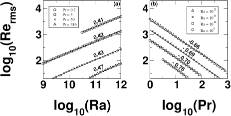
Figure 4: Reynolds number variance $\mbox{Re}_{rms}$ based on the root mean square velocity as function of (a) Ra and (b) Pr.

Mean reversal frequency: The abrupt change of $X(\tau)$ with $\tau$ [cf. figure 2(b)] suggests that the wind switching can be approximately considered as an almost instantaneous event represented by the moment at which it occurs. Here, we follow Sreenivasan et al. Sreenivasan/wind/PRE/2002 and define $t^{\prime}_{n}$ as the interval between an arbitrary origin in time and the nth wind reversal. Similarly as in Sreenivasan/wind/PRE/2002 , we also find a linear relation $t^{\prime}_{n}\sim n$, which suggests a mean interval $\bar{t^{\prime}}$ between reversals. In this way, we define $\omega=1/\bar{t^{\prime}}$ as the mean reversal frequency, and its dimensionless counterpart as $\tilde{\omega}=\omega\,L^{2}/\nu$.

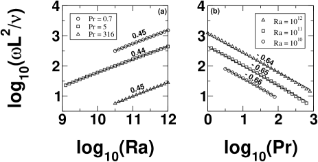
Figure 5: Mean reversal frequency as function of (a) Ra at fixed Pr and (b) Pr for given Ra.

Figure 5 shows that $\tilde{\omega}\sim\mbox{Pr}^{-(0.65\pm 0.01)}\,\mbox{Ra}^{0.44\pm 0.01}$. To our knowledge, the only experimental measurement of the reversal frequency has been carried out in cryogenic helium gas Sreenivsan/Niemela/frequency/private , namely $\tilde{\omega}\sim\mbox{Ra}^{0.71}$ for $\mbox{Pr}=0.75$ and $2.1\times 10^{8}\leq\mbox{Ra}\leq 1\times 10^{13}$. The disagreement between our result and the particular measurement suggests that a model based on only 3-modes for the plumes is quantitavely inadequate. In this qualitative sense, our simple deterministic system well mimics the dynamics of reversals, and is a complementary approach to the stochastic model of noise-induced switchings between two metastable states Sreenivasan/wind/PRE/2002 . Here, the Lorenz attractor itself captures the bistable transitions, but a more quantitative description of the reversal phenomenon (also including the rotation scenario) would involve a subtle combination of deterministic chaos and noise. This could be done in the spirit of ref. Silchenko/PRE/2002 (sec. III C), and is left for future work.

- (1) R. Krishnamurti, L. N. Howard, Proc. Natl. Acad. Sci. USA 78, 1981 (1981).
- (2) H. D. Xi, S. Lam, K. Q. Xia, J. Fluid Mech. 503, 47 (2004).
- (3) R. Benzi, Phys. Rev. Lett. 95, 024502 (2005).
- (4) K. R. Sreenivasan, A. Bershadskii, J. J. Niemela, Phys. Rev. E 65, 056306 (2002).
- (5) J. J. Niemela, L. Skrbek, K. R. Sreenivasan, R. J. Donnelly, J. Fluid Mech. 449, 169 (2001).
- (6) S. Cioni, S. Ciliberto, J. Sommeria, J. Fluid Mech. 335, 111 (1997).
- (7) Y. Tsuji, T. Mizuno, T. Mashiko, and M. Sano, Phys. Rev. Lett. 94, 034501 (2005).
- (8) E. Brown, A. Nikolaenko, and G. Ahlers, Phys. Rev. Lett. 95, 056101 (2005).
- (9) E. van Doorn, B. Dhruva, K. Sreenivasan, V. Cassella, Phys. Fluids 12, 1529 (2000).
- (10) G. A. Glatzmeier, R. C. Coe, L. Hongre, P. H. Roberts, Nature 401, 885 (1999).
- (11) U. Hansen, D.A. Yuen, S.E. Kroening, Geophys. Astrophys. Fluid Dynamics 63, 67 (1992)
- (12) A. Furukawa, A. Onuki, Phys. Rev. E 66, 016302 (2002)
- (13) S. Grossmann, D. Lohse, Rayleigh-Prandtl number dependent phase diagram for strong thermal convection, in High Rayleigh Number Convection, International Workshop, September 3-5, 2001, Ilmenau, Germany.
- (14) D. Lohse, Phys. Rev. Lett. 73, 3223 (1994).
- (15) S. H. Strogatz, Nonlinear dynamics and chaos, Perseus Books, Reading (1994).
- (16) M. Kolár, G. Gumbs, Phys. Rev. A 45, 626 (1992).
- (17) E. N. Lorenz, J. Atmos. Sci. 20, 130 (1963).
- (18) J. B. McLaughlin, P. C. Martin, Phys. Rev. A 12, 186 (1975).
- (19) M. Gorman, P. J. Widmann, K. A. Robbins, Phys. Rev. Lett. 52, 2241 (1984).
- (20) P. Ehrhard, U. Müller, J. Fluid Mech. 217, 487 (1990).
- (21) What however our modified Lorenz system has in common with the original one is that it is not suited to make statements on the heat flux in the turbulent regime.
- (22) W. H. Press, S. A. Teukolsky, W. T. Vetterling, B. P. Flannery, Numerical Recipes in C, Cambridge University Press (1992).
- (23) S. Grossmann, D. Lohse, J. Fluid Mech. 407, 27 (2000); Phys. Rev. Lett. 86, 3316 (2001); Phys. Rev. E 66, 016305 (2002), Phys. Fluids, 16, 4462 (2004).
- (24) H. R. Dullin, S. Schmidt, P. H. Richter, S. Grossmann, Chaos, submitted (2005).
- (25) S. Lam, X.D. Shang, S.Q. Zhou, K.Q. Xia, Phys. Rev. E 65, 066306 (2002).
- (26) J. J. Niemela, K. R. Sreenivasan, private communication.
- (27) A. Silchenko, C.-K. Hu, Phys. Rev. E 63, 041105 (2001).