A study on a self-organized criticality in a dynamical many-body system

Abstract

A novel mechanism for the generation of self-organized criticality (SOC) is discussed in terms of the coupled-vibration model where the total system is forced under the uniform expansion of the Hubble type. This system shows a robust SOC behavior while the maximum size of the fluctuation, number of correlated particles in it and the temporal size of the system evolve as a function of time.

Observation of the ubiquitous manifestation of fractal structure in nature is one of the most fascinating findings in non-linear science Mandelbrot (1983). One direction for the understanding of the origin of its manifestation was offered in Bak et al. (1987, 1988) with the concept of self-organized criticality (SOC). It was argued there that the scaling properties of the attractor is insensitive to the parameter of the model, which shows a robustness of the criticality. Since then, many models of cellular-automata were studied Jensen (1998); Turcotte (1999), where another characteristic feature is that the external driving of the system is much slower than the internal relaxation processes.

The separation of external and internal time-scales, however, is not always a guiding principle for the pattern formation. Turbulent flow, for example, seems to have more dynamical origin. In this respect, we will seek a SOC state where the external driving of the system has a comparable time scale to that of the internal motion. The disappearance of the characteristic length scale and the robustness are used to characterize SOC. As a typical example which shows this feature, we propose a homogeneously expanding lattice model which was motivated by our previous study Chikazumi and Iwamoto (2004). We define a one-dimensional version of the previous modelChikazumi and Iwamoto (2004) and make an anatomy of SOC formation when the many-particle system is put in a mechanically unstable state.

Our model is based on an expanding one-dimensional coupled-vibration model. The chain is composed of $N_{0}+2$ particles of equal mass $m$, coupled with the nearest neighbor particles by a finite-depth potential. This chain is forced to obey a uniform expansion of the Hubble-type Chikazumi and Iwamoto (2004). Physically important feature is that as the lattice spacing increases, each particle at the lattice point becomes unstable against the motion to right or to left, forming a cluster. Although the following discussion will be applied to rather general class of interactions, we take Lennard-Jones (L-J) potential as a prototype Chikazumi and Iwamoto (2004).

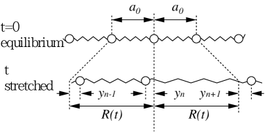
Figure 1: Sketch of the extended chain used. At equilibrium, random and small fluctuations are assumed.

We analyze a motion of mono-particle one-dimensional lattice with a lattice spacing $R$ larger than its equilibrium separation $a_{0}$ as is given schematically in FIG.1. The expansion of the lattice is described with the relation,

$$R(t)=a_{0}(1+ht)$$ (1)

where the Hubble constant $h$ is introduced. This condition is satisfied by putting the initial velocities to each particle together with the corresponding velocities to the boundaries to which $0-th$ and $(N_{0}+1)th$ particles are held fixed. The equation of motion of this system is written as

$$m\frac{d^{2}y_{n}}{dt^{2}}=V^{\prime}(R+y_{n+1}-y_{n})-V^{\prime}(R+y_{n}-y_{n-1}),$$ (2)

where $y_{n}$ stands for a displacement of n-th lattice particle from its lattice point and $V^{\prime}$ is the derivative of the inter-particle potential. Suffix n runs from 1 to $N_{0}$ in this equation. We assume this potential $V$ is given by the Taylor polynomial expansion around $R$ for small displacement $r$,

$$V^{\prime}(R+r)\approx V^{\prime}(R)+V^{\prime\prime}(R)r.$$ (3)

Inserting this form to (2), we obtain

$$m\frac{d^{2}y_{n}}{dt^{2}}=\kappa(2y_{n}-y_{n+1}-y_{n-1}),$$ (4)

where we put $\kappa$ for $-V^{\prime\prime}(R)$. It should be noted here that the $\kappa$ is always negative when we deal with the stationary oscillation where $R=a_{0}$. On the other hand, for L-J potential, it becomes positive when $R\geq 1.11a_{0}$. In the following discussion, we mainly treat this situation and thus we assume $\kappa$ is positive.

To solve (4), we assume the following standard form of the solution,

$$y_{n}=a\exp(ikn\mp\omega t).$$ (5)

Inserting this form to eq.(4), we get,

$$\omega^{2}=\frac{4\kappa}{m}\sin^{2}\frac{k}{2}.$$ (6)

This dispersion relation has the same form as for the normal-mode analysis for the equilibrium oscillation except for the fact that the motion of the lattice particle $y_{n}$ is not oscillatory but divergent as is clear from eq.(5). When we calculate the second derivative of $y_{n}$ in (4), the following derivative appears,

$$d(\omega t)/dt=\omega+d\omega/dt\times t.$$ (7)

For a non-singular form of $\omega$, the second term in the rhs is smaller than the first term for sufficient small value of t. Therefore, we can justify the dispersion relation (6) under the condition $y_{n}\ll R(t)$ and for short-time regime.

The solution of the equation (4) for small displacement and for small t, under the boundary condition,

$$y_{0}=0=y_{N_{0}+1}$$ (8)

is written as

$$y_{n}=a\exp(\mp\omega t)\sin(kn),$$ (9)

where $a$ is a constant. In this form, the boundary condition for n=0 is automatically satisfied and for n=$N_{0}$+1, we obtain a relation,

$$k=\frac{\pi\nu}{N_{0}+1}.\,\,\,\,(\nu=1,2,...N_{0})$$ (10)

For convenience, we rewrite (10) and (6) in the form,

$$k_{\nu}=\frac{\pi\nu}{N_{0}+1},$$ (11)

$$\omega_{\nu}^{2}=\frac{4\kappa}{m}\sin^{2}\frac{k_{\nu}}{2}. \,\,\,\,(\nu=1,2,...N_{0})$$ (12)

The general solution is written down in the form

$$y_{n}=\sum A_{n\nu}Q_{\nu},$$ (13)

$$A_{n\nu}=\sqrt{\frac{2}{N_{0}+1}}\sin\frac{\pi n\nu}{N_{0}+1},$$ (14)

$$Q_{\nu}=a_{\nu}[\exp(\omega_{\nu}t)+b_{\nu}\exp(-\omega_{\nu}t)]/2,$$ (15)

where $a_{\nu}$ and $b_{\nu}$ are free parameters that fit the 2$N_{0}$ initial conditions for $N_{0}$ particles.

In the $\nu$-th normal-mode for the longitudinal motion (identify $nR$ as x-coordinate), the following number of particles $n_{\nu}$ are compressed or stretched as a whole,

$$n_{\nu}=\frac{(N_{0}+1)}{\nu}=\frac{\lambda_{\nu}(t)}{2R(t)},$$ (16)

where $\lambda_{\nu}$ is a wavelength for the $\nu$-th mode expressed as $(2L(t))/\nu$ by using the total length of the chain $L(t)$ at time t. Therefore, the correlation of $n_{\nu}$ particle is produced by the $\nu$-th normal mode. The growth of the $\nu$-th normal mode is governed by (15) and is exponentially divergent. The time ordering of the growth is known from eqs.(11) and (12). For larger $\nu$, the $k_{\nu}$ value becomes larger , which leads to larger $\omega_{\nu}$ value. It means that the exponential growth of the fluctuation occurs stepwise, from the highest frequency to the lower frequency, in other word, from the shortest wavelength to the larger wavelength. When we start from the random small fluctuations of the particles’ position or velocities or both, it corresponds to the fact that $a_{\nu}$ in (15) stands for a white spectrum.

Above discussion is applicable only for small fluctuation and for short-time behavior. In other word, it is a linearized discussion because we assumed no coupling between various normal modes. For the analysis of SOC, however, we have to go into finite-time and nonlinear regime. We first postulate the following three hypotheses: 1) Even at finite-time, the formation of cluster starts from small particle number to large particle number. 2) At the time when $n_{\nu}$ correlation just starts, its spatial size $\delta_{c}(t)$ is characterized by the relation

$$\delta_{c}(t)\equiv\lambda_{\nu}(t)/2=n_{\nu}(t)\times R(t)$$ (17)

3) The spatial size of the fluctuation for $n_{\nu}$ particles is approximately conserved even at later time.

The hypothesis 1) and 2) are taken from the linear regime from (16). The hypothesis 3) means that the size of the clusters are frozen at the time of its formation, without stretching or shrinking at later time. It means that at the start of the $n_{\nu}$ correlation and later on, $n_{\nu}$ particles are trap in the mutual attractive interaction bloc, free from the uniform expansion to which $n_{\nu}$ particles followed before. Since we assume no energy dissipation, the time-averaged spatial size of the bloc is conserved. It should be noted that when $n_{\nu}$ correlation starts, correlations of smaller particles are preserved in the $n_{\nu}$ correlation, forming a nesting-boxes structure.

Next task is to determine the dependence of the $\delta_{c}(t)$ and $n_{\nu}(t)$ on $R(t)$ which satisfies (17). We postulate the following relation to generate the solution of (17).

$$\frac{dn_{\nu}(t)}{d\delta_{c}(t)}=\gamma/R(t)$$ (18)

where $\gamma$ stands for a non-dimensional constant. The form of lhs was adopted because we study a growth process of $n_{\nu}$ and $\delta_{c}(t)$. The form of rhs is assumed because the lhs has the dimension of [length]^-1 and we know that the system has a lattice unit parameter $R(t)$ which has the dimension of [length]. The parameter $\gamma$ is a function of the Hubble constant $h$ in such a way that $\gamma\rightarrow 0$ for large value of $h$ and $\gamma\rightarrow 1$ for small value of $h$. The former condition corresponds to an enlarged copy of the system discussed in Chikazumi and Iwamoto (2004) and the latter to a system where there happens one break of the chain and the left and the right matters move to the left and to the right without changing their sizes. Thus the assumption of (18) is that lhs is proportional to the bulk ratio $R(t)$, cf.(17), times $\gamma$, which stands for the amount of tension due to the competition of expanding motion and the internal attraction. The condition that this $\gamma$ is a constant is the condition of realizing the SOC, because we will see in FIG.3 that the relation (18) is found to be well satisfied in the numerical calculations.

Using (17), the solution of (18) is written as

$$n_{\nu}(t)=const\times\delta_{c}(t)^{\gamma}.$$ (19)

This $n_{\nu}$ is directly related to the box-counting number $N(t)$ for the size of $\delta_{c}$, as is given by the relation,

$$N(t)=N_{0}/n_{\nu}(t)=N_{0}\delta_{c}(t)^{-\gamma}/const,$$ (20)

which is clear from (17). The relation (19) means that the correlation length is expressed as a power of the distance, a typical feature of phase transition point. Here, $n_{\nu}$ is considered as distance measured in unit of lattice spacing $R(t)$. Since $\gamma$ depends on the expansion speed, the criticality is not universal here but SOC is well satisfied because the system without fail goes into the critical state that satisfies the power-law relation (19). The fact that all the complexity of the non-linear effect is simply written in a form (18) is astonishing.

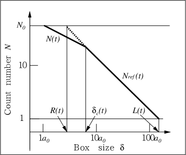
Figure 2: Relation of $\delta_{c}(t)$, $N(t)$ and $R(t)$ in the graph of log-log sale for the box size $\delta$ and count number $N$. Cross-over effect and the maximum fluctuation are shown.

Inserting (19) into (17), we can get the explicit expression of $\delta_{c}(t)$ in terms of $R(t)$. We can also obtain $\delta_{c}(t)$ in terms of the relation among $\delta_{c}(t)$, $N(t)$ and $R(t)$ with the help of FIG.2 drawn in log-log scale with the abscissa corresponding to box size $\delta$ and the ordinate, to the count number $N$. In this figure, the trace of (20) is shown by the solid line $N(t)$ up to a specific time t. For a fixed time, the maximum size of the fluctuation is $\delta_{c}(t)$, beyond which the box counting number should follow the one-dimensional line $N_{ref}(t)$ shown in the figure. That is, we define $\delta_{c}(t)$ and $N(t)=N_{0}/n_{\nu}(t)$ as x- and y-coordinates of this cross point. The line $N_{ref}(t)$ should pass through the count of unity when the box size $\delta$ coincides with the total chain length L,

$$\log{N_{ref}(t)}=-\beta(\log{\delta}-\log{L(t)}),$$ (21)

where $\beta$ stands for 1 in our case and 3 in the 3-dimensional case.

The value of $\delta_{c}(t)$ is the x-coordinate of the cross point of the line (20) and the line (21) which is expressed as

$$\delta_{c}(t)^{\beta-\gamma}=const\times R(t)^{\beta},$$ (22)

which has the same form as the short time behaviour seen in dynamical scaling Vicsek and Family (1984). For general spatial dimension, relation (17) is replaced by

$$\delta_{c}(t)^{\beta}=n_{\nu}(t)\times R(t)^{\beta},$$ (23)

where $\beta$=3 applies to our previous calculation Chikazumi and Iwamoto (2004).

The third hypothesis we postulated is a key to get the fractal growth in SOC state and the normal fractal dimension calculation for a fixed system. Because of this hypothesis, the fractal structure formed in SOC is frozen out. The fact that the growth of the maximum fluctuation in our model is closely related to a cross-over effect, is a typical feature of our dynamical SOC state.

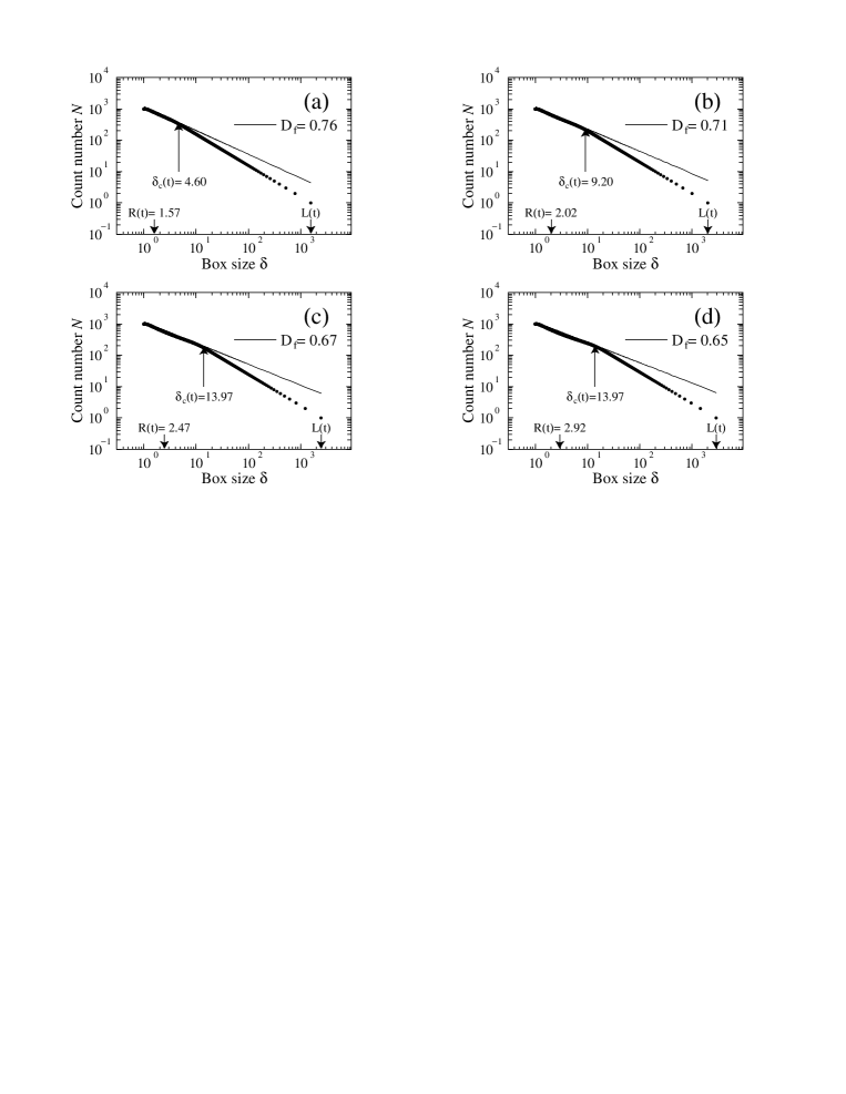
Figure 3: Numerical simulation of the box-counting for the system for $h$=0.1, $N_{0}$=1000 averaged over 10 events for fixed boundary condition and for nearest neighbor interaction. Each panel corresponds to the time sequence of the expansion of the system.

Now we are ready to check our three hypotheses and the postulation (18) with a help of the numerical simulation for linear chain interacting with L-J potential The unit of length $\sigma$ is the distance at which the potential changes sign and the energy unit $\epsilon$ is the depth of the potential. The time unit $t_{0}$ is composed as $t_{0}=\sqrt{\sigma^{2}m/48\epsilon}$. Before physical discussion, we first check the dependence of the results on the number of particles $N_{0}$. We performed the box-counting method with 100 particles and 1,000 particles. The results hardly change when we averaged over 10 independent trials for the different initial states. For boundary conditions, we used a fixed boundary condition (8) in our formalism. We checked the periodic boundary condition to simulate the infinite system Chikazumi and Iwamoto (2004). We also checked the results when we include only the nearest neighbor interaction or allow the next neighbor one. We found that such changes altogether cause at most 1% change of the fractal dimension value.

In FIG.3, we show the box counting plot for the system for $h$=0.1, $N_{0}$=1000 averaged over 10 events for fixed boundary condition and for nearest neighbor interaction. The value of the lattice spacing is shown in these figures by $R(t)$ in unit of the equilibrium lattice spacing. As we see in this figure, the fractal structure is clearly seen up to the cross-over point, which extends as $R(t)$ increases. The linearity of the slope, which is closely related to the assumption of constant $\gamma$ in eq.(18) is well realized in this figure. The FIG.3(d) corresponds to $R(t)$=2.92, which exceeds the cut-off length 2.5 of our Lennard-Jones potential Chikazumi and Iwamoto (2004). In this situation, the formation of a cluster in our formalism is not physically applicable and therefore, the $\delta_{c}$ value of FIG.3(c), which is just before $R(t)$ exceeds the cutoff length is shown. Actually, the behavior beyond this $\delta_{c}$ value starts to wave from the linear line. Another important tendency is the gradual decrease of the slope parameter as time proceeds. The change of this value is interpreted as due to the decrease of the stiffness parameter $\kappa$ as $R(t)$ increases. This causes the decrease of the clustering force compared with the expansion induced by $h$, which leads to a smaller fractal dimension $\gamma$.

The same degree of good fitting with two linear lines is obtained for h=0.2,0.3 and 0.4. As is expected, the fractal dimension becomes smaller, the larger the $h$ values. For example, the slope parameters (fractal dimensions) corresponding to FIG.3(c) ($R(t)=2.47$) are 0.67, 0.61, 0.56, 0.51 for $h$=0.1, 0.2, 0.3 and 0.4. Another important factor which determines the slope is the strength of the initial fluctuation. We adopted the initial conditions that $N_{0}$ particles are initially at rest and are located around the lattice site randomly within $\pm p\%$ of the original lattice spacing. This condition, when we remember eq.(15), corresponds to $b_{\nu}=1$ and the strength of random variable $a_{\nu}$ is proportional to $p$. The results shown in FIG.3 corresponds to $p$=5. The fractal dimension for $p$=5 $\sim 10$ is rather stable, changes less than 3 % like three dimensional calculation in Chikazumi and Iwamoto (2004). However, when we reduce $p$ to smaller values, the fractal dimension becomes smaller, approaching to zero for small fluctuation limit. It is because $a_{\nu}$ value in (15) becomes smaller for smaller initial fluctuation and the start of $n_{\nu}$ correlation is delayed with respect to time, which means the decrease of the slope of the fractal line. The numerical calculations show essentially the same results as in the 3-dimensional case Chikazumi and Iwamoto (2004), which suggests that this kind of SOC is common to any dimension.

In conclusion, our coupled linear-chain model with finite-range interaction, when forced under the uniform expansion of the Hubble type, leads to a robust SOC state and shows a fractal structure and a cross-over effect. The slope (box-counting fractal dimension) depends on the expansion speed and the strength of the initial fluctuations. This SOC state in the dynamical many-particle system differs from the standard SOC in two respects, 1) relative time scales of external and internal motions, 2) existence of a clear cross-over effect, that has a possibility to open a new window towards our understanding of fractal structure in nature.

We thank Dr. T. Yokota for useful discussions.

References

- Mandelbrot (1983) B. Mandelbrot, The Fractal Geometry of Nature (Freeman, New York, 1983).
- Bak et al. (1987) P. Bak, C. Tang, and K. Wiesenfeld, Phys.Rev.Lett. 59, 381 (1987).
- Bak et al. (1988) P. Bak, C. Tang, and K. Wiesenfeld, Phys.Rev.A. 38, 364 (1988).
- Jensen (1998) H. Jensen, Self-Organized Criticality (Kambridge University Press, 1998).
- Turcotte (1999) D. Turcotte, Rep.Prog.Phys 62, 1377 (1999).
- Chikazumi and Iwamoto (2004) S. Chikazumi and A. Iwamoto, Chaos, Solitons & Fractals, in press; arXiv:nlin.AO/0401019 v3 26 Jan 2004 (2004).
- Vicsek and Family (1984) T. Vicsek and F. Family, Phys.Rev.Lett. 52, 1669 (1984).