The $N$-Soliton of the Focusing Nonlinear Schrödinger Equation for $N$ Large

Abstract.

We present a detailed analysis of the solution of the focusing nonlinear Schrödinger equation with initial condition $\psi(x,0)=N\,{\rm sech}(x)$ in the limit $N\rightarrow\infty$. We begin by presenting new and more accurate numerical reconstructions of the $N$-soliton by inverse scattering (numerical linear algebra) for $N=5$, $10$, $20$, and $40$. We then recast the inverse-scattering problem as a Riemann-Hilbert problem and provide a rigorous asymptotic analysis of this problem in the large-$N$ limit. For those $(x,t)$ where results have been obtained by other authors, we improve the error estimates from $O(N^{-1/3})$ to $O(N^{-1})$. We also analyze the Fourier power spectrum in this regime and relate the results to the optical phenomenon of supercontinuum generation. We then study the $N$-soliton for values of $(x,t)$ where analysis has not been carried out before, and we uncover new phenomena. The main discovery of this paper is the mathematical mechanism for a secondary caustic (phase transition), which turns out to differ from the mechanism that generates the primary caustic. The mechanism for the generation of the secondary caustic depends essentially on the discrete nature of the spectrum for the $N$-soliton, and more significantly, cannot be recovered from an analysis of an ostensibly similar Riemann-Hilbert problem in the conditions of which a certain formal continuum limit is taken on an ad hoc basis.

1. Introduction

It is well known (see, e.g., [13]) that the solution of the initial-value problem for the focusing nonlinear Schrödinger equation

(1) $$i\psi_{t}+\frac{1}{2}\psi_{xx}+|\psi|^{2}\psi=0$$

with initial data

(2) $$\psi(x,0)=N\,\text{sech}(x)$$

is a special solution called the $N$-soliton. This solution is rapidly decreasing in $|x|$ and periodic in $t$ with period independent of $N$. To further describe this solution, we recall that (1) is exactly solvable via the inverse-scattering framework introduced by Zakharov and Shabat in [16]. There are three steps in the procedure:

1. forward scattering — the initial data generates the scattering data which consists of eigenvalues, proportionality constants, and a reflection coefficient;

2. time evolution — the scattering data have a simple evolution in time;

3. inverse scattering — the solution of the partial differential equation at later times is reconstructed from the time-evolved scattering data.

For the special initial data (2), Satsuma and Yajima [13] have shown that the reflection coefficient is identically zero and there are $N$ purely imaginary eigenvalues. Such a reflectionless solution whose eigenvalues have a common real part is an $N$-soliton.

Here, using the the inverse-scattering framework for (1)–(2), we study the $N$-soliton in the limit $N\to\infty$. For the first few positive integer values of $N$, it is possible to write down explicit formulas for these exact solutions of the nonlinear partial differential equation (1). However, these formulae rapidly become unwieldy. Even for $N=3$, the formula is already quite complicated and hard to analyze. Amazingly, while these formulae grow increasingly complicated as $N$ increases, it is also true that certain orderly features emerge in the limit $N\to\infty$.

As a first step, we rescale $\psi$ and $t$ in (1)–(2) to make the initial amplitude independent of $N$ and the period proportional to $N$, and we arrive at

(3) $$i\hbar\psi_{t}+\frac{\hbar^{2}}{2}\psi_{xx}+|\psi|^{2}\psi=0,$$

(4) $$\psi(x,0)=A\,\text{sech}(x),$$

where $\hbar=\hbar_{N}:=A/N$ and $A>0$. Studying the large-$N$ limit of the $N$-soliton is thus equivalent to studying the semiclassical ($\hbar\downarrow 0$) limit of (3)–(4). A feature that emerges in the limit is the sharpening boundaries in the $(x,t)$-plane that separate different behaviors of the solution. Two such “phase transitions” were noticed in the numerical experiments of Miller and Kamvissis [12], and the first, a so-called primary caustic curve in the $(x,t)$-plane, was rigorously explained by Kamvissis, McLaughlin, and Miller [10]. Here, our main result is a description of the mechanism for the observed second phase transition; it differs from the first one.

We use two formulations of the inverse-scattering step to study the limiting behavior of (3)–(4). When, as is the case here, the reflection coefficient is absent, the algebraic-integral system that one expects to solve to reconstruct the solution of (3) for generic initial data reduces to a linear algebraic system. We derive such a system in § 2 below. We also show, in § 3.1, that the reconstruction step can be cast as a discrete Riemann-Hilbert problem for a meromorphic $2\times 2$ matrix unknown. We use the linear algebraic system as a basis for numerically computing the $N$-soliton while the Riemann-Hilbert formulation provides the starting point for our asymptotic analysis. In either case, the reconstruction of the solution begins with the eigenvalues

(5) $$\lambda_{N,k}:=iA-i\left(k+\frac{1}{2}\right)\hbar_{N},\quad k=0,\ldots,N-1,$$

and the proportionality constants

(6) $$\gamma_{N,k}:=(-1)^{k+1},\quad k=0,\ldots,N-1.$$

In § 3 we describe how to explicitly modify the discrete Riemann-Hilbert problem we obtain in § 3.1 to arrive at an equivalent problem that is conducive to rigorous asymptotic analysis in the limit $N\rightarrow\infty$ (or equivalently $\hbar\rightarrow 0$). In § 3.2 we convert the discrete Riemann-Hilbert problem into a conventional Riemann-Hilbert problem for an unknown with specified jump discontinuities across contours in the complex plane. Next, we show how to “precondition” the resulting Riemann-Hilbert problem for the limit $N\rightarrow\infty$ by introducing a scalar function $g(\lambda)$ that is used to capture the most violent asymptotic behavior so that the residual may be analyzed rigorously. In some cases, the function $g(\lambda)$ leads to an asymptotic analysis in the limit $N\rightarrow\infty$ based on the theta functions of hyperelliptic Riemann surfaces of even genus $G$, and in such cases the function $g(\lambda)$ can be constructed explicitly, as we show in § 3.4. This construction forces certain dynamics in $(x,t)$ on the moduli (branch points) of this Riemann surface, and in § 3.4.1 we show that the moduli satisfy a universal system of quasilinear partial differential equations in Riemann-invariant form, the Whitham equations. The success or failure of the function $g(\lambda)$ constructed in this way in capturing the essential dynamics as $N\rightarrow\infty$ hinges upon certain inequalities and topological conditions on level curves that are described in § 3.4.2. With a function $g(\lambda)$ in hand that satisfies all of these conditions, we may proceed with the asymptotic analysis, which is based on a steepest descent technique for matrix Riemann-Hilbert problems developed by Deift and Zhou [7]. We summarize these steps in § 3.5, § 3.6, and § 3.7.

The theory outlined above provides, through a handful of technical modifications, a refinement of results previously obtained by Kamvissis, McLaughlin, and Miller [10]. The key techincal improvements are the avoidance, through a dual interpolant approach developed in [11] and [1], of a local parametrix near the origin in the complex plane and the explicit and careful tracking of the errors in replacing a distribution of point masses representing condensing soliton eigenvalues by its weak continuum limit, encoded in certain functions $S(\lambda)$ and $T(\lambda)$. These extra steps allow us to deduce the same asymptotic formulae obtained in [10] governing the semiclassical limit up to and just beyond the primary caustic curve in the $(x,t)$-plane, but with an improved error estimate that is $O(\hbar)$ (which beats the $O(\hbar^{1/3})$ estimate in [10]).

It is fair to say that much of the work in analyzing the $N$-soliton in the limit of large $N$ comes about from vanquishing the poles representing the soliton eigenvalues from the matrix-valued Riemann-Hilbert problem that represents the inverse-scattering step. In some sense, the poles disappear with the interpolation step that converts the discrete Riemann-Hilbert problem with poles but no jump discontinuities into one with jump discontinuities and no poles. On the other hand, this is only a partial solution, since the jump matrix relating the boundary values taken along a curve of jump discontinuity extends from this curve as an analytic function with poles at the soliton eigenvalues. However, as long as the jump contour remains bounded away from these poles, it is a reasonable approximation that can be controlled rigorously to replace the jump matrix by another one in which the distribution of poles is “condensed” into a continuous distribution with an analytic density. Making this replacement on an ad hoc basis changes the problem. We refer to this changed inverse-scattering problem as the formal continuum-limit problem and we discuss it briefly in § 3.8. The formal continuum-limit problem indeed gives the correct asymptotics of the $N$-soliton and related initial data for the semiclassical focusing nonlinear Schrödinger equation (3) subject to the above caveat, and it even forms the starting point for the analysis of [15].

Interestingly, the choice of the function $g(\lambda)$ turns out to have the following two properties:

• It depends only on the analytic weak limit of the discrete distribution of soliton eigenvalues.

• It determines the contours of the Riemann-Hilbert problem of inverse scattering, and in particular their relation to the locus of accumulation of the discrete soliton eigenvalues.

So, from the first property, $g(\lambda)$ does not know about the poles of the jump matrix, and from the second property it chooses the contours appropriate for the asymptotic analysis. It is therefore possible that the contours selected by choice of $g(\lambda)$ could cross the locus of accumulation of discrete eigenvalues. And once the contours are no longer bounded away from the poles, the formal continuum-limit problem is not the correct model for inverse scattering.

It turns out that, in the region beyond the primary caustic curve, this actually happens. In other words, the dependence of the function $g(\lambda)$ on $(x,t)$ predicts a contour that as $t$ increases passes through the branch cut that is the continuum limit of the pole distribution. At this point, the rigorous analysis must break down. Significantly, however, this is not the mechanism for further phase transitions. It turns out that the difficulty is a technical one that can be removed with the further use of the multi-interpolation method developed in [11] and [1]. The additional steps that are required to surmount this crisis, and to therefore prove that there is no phase transition when curves determined from the function $g(\lambda)$ cross the pole locus, are described in § 3.9.

The analysis described in § 3.9 is new, and one of the new features is the appearance of a new inequality that must be satisfied by the function $g(\lambda)$ on certain contours. It turns out that the failure of this inequality is the mathematical mechanism for the next phase transition of the $N$-soliton, a secondary caustic curve in the $(x,t)$-plane.

Before studying the secondary caustic, we discuss briefly in § 4 the quiescent region of the $(x,t)$-plane before the primary caustic curve. We recall in § 4.1 some information from [10] about the relation between the dynamics of the $N$-soliton in this region and a family of hyperelliptic Riemann surfaces of genus zero. We also discuss the mathematical mechanism behind the primary caustic phase transition, which turns out to correspond to an instantaneous jump from genus zero to genus two. Then, in § 4.2 we analyze the Fourier power spectrum of the $N$-soliton in the region before the primary caustic, and show that its evolution is consistent with the supercontinuum generation phenomenon of current interest in optical science (see below).

In carrying out a study of the $N$-soliton for large $N$, three different computational techniques come to mind:

1. Direct numerical simulation of the initial-value problem for the focusing nonlinear Schrödinger equation (3) in the semiclassical limit. By adapting discretization methods to this problem, it is possible to study the dynamics of the $N$-soliton as well as much more general initial data, and also non-integrable variants of (3). However, these methods are severely constrained in the limit of interest due to numerical stiffness, and worse yet, modulational instability that is exponentially strong in $N$. See [2, 5, 3, 4].

2. Numerical solution of the inverse-scattering problem for the focusing nonlinear Schrödinger equation. This method applies only to the integrable equation (3), and like the direct numerical simulation method is also ill-conditioned in the semiclassical limit. However, it affords an important advantage over direct numerical simulation, namely that the solution is calculated independently for each $(x,t)$, and therefore roundoff errors do not accumulate.

3. Numerical construction of the function $g(\lambda)$. This method also applies only to the integrable equation (3), and it is further constrained in that it is only meaningful in the semiclassical limit. However, it specifically takes advantage of the mathematical structure of this limit, and consequently the numerical calculation is extremely well-conditioned.

In § 5, we take the third approach and use numerical methods to solve for the function $g(\lambda)$ in the region between the primary and secondary caustics for the $N$-soliton. While a numerical calculation, this is clearly fundamentally different from either the numerical solution of linear algebra problems equivalent to inverse scattering for the $N$-soliton as in § 2, or direct numerical simulation of the initial-value problem for (3) corresponding to the $N$-soliton. It is with the help of these calculations that we observe the crossing of the pole locus (which does not correspond to the secondary caustic, as can be seen once the analysis is modified as in § 3.9) and ultimately the violation of the new inequality introduced in § 3.9 (which causes the secondary caustic phase transition).

In § 6 we take up the question of exactly what happens to the $N$-soliton immediately beyond the secondary caustic curve in the $(x,t)$-plane. We characterize the secondary caustic (failure of the new inequality from § 3.9) as the occurance of a critical point on a level curve defining the boundary of the region in the complex plane where the relevant inequality holds. We then make the guess that the failure of $g(\lambda)$ corresponding to a Riemann surface of genus two in this new way is resolved by going over to a formula for $g(\lambda)$ corresponding to a Riemann surface of genus four, but with significantly different topological features than in the (hypothetical) case that genus two fails due to the violation of the same inequality that leads to the primary caustic. We construct $g(\lambda)$ in this new situation, and obtain an implicit description of the moduli of the corresponding genus four Riemann surface. These are new formulae that have a different character than those obtained earlier. We then prove that these new formula provide another solution to the same type of Whitham equations that govern the moduli in the case of simpler contour topology.

We conclude the paper with some hypotheses regarding further phase transitions (higher-order caustics) for the $N$-soliton and related initial-value problems for (3), and by stressing once again that the phenomenon of the secondary caustic (and possibly further phase transitions) is fundamentally linked to the discrete nature of the eigenvalue distribution, which forces modifications to the analysis as described in § 3.9, and introduces coincident inequalities to be satisfied by $g(\lambda)$. These inequalities are simply not part of the asymptotic theory of the formal continuum-limit problem discussed in § 3.8, and therefore the latter problem is unable to correctly predict the secondary caustic. This came as some surprise to us, as we and other authors had always assumed that either the formal continuum-limit problem governs the dynamics for all time or that the secondary caustic occurs upon crossing the locus of eigenvalues. Both of these are incorrect.

The problem (3) for small $\hbar$ is relevant as a model for the propagation of light pulses in optical fibers that have the property of weak (because $\hbar$ is small) anomalous dispersion. There has always been great interest in optical fibers with weak dispersion. Initially this was because when such fibers are operated in the linear regime (small amplitude) the propagation is immune to dispersive spreading of pulses that is considered to degrade a data stream. For long fiber links, however, the theory of linear propagation becomes inadequate due to the accumulation of weakly nonlinear effects. More recently these fibers have become important again because it became clear that advantage could be taken specifically of the nonlinearity. Indeed, when operated in the weakly nonlinear regime (moderate amplitude) nonlinear effects are much stronger compared to linear effects and therefore propagation in such fibers can drastically alter the power spectrum of a signal, possibly in a useful way. Indeed, one of the applications envisioned for weakly dispersive fibers is so-called supercontinuum generation (see, for example, [6, 8]) in which a nearly monochromatic laser source is coupled into the fiber and spectrally broadened under propagation so that the output is a coherent source of white light. The output can then be filtered to produce coherent light of virtually any frequency, which is desirable for wavelength division multiplexing telecommunication systems. The most promising current technology for creating optical fibers with very low dispersion, in both the normal and anomalous regimes, is based on photonic crystal fibers, which are made from fiber preforms with extremely complicated cross sections. The complexity of the cross section is preserved to the microscopic level upon drawing the fiber (carefully stretching the cylindrical fiber preform along its axis until an optical fiber results), and as the possibilities for cross sections go far beyond the traditional core/cladding/jacket step-index model it is possible to engineer fibers with properties thought impossible until recently [9].

In this paper, we make frequent use of the three Pauli matrices:

(7) $$\sigma_{1}:=\left[\begin{array}[]{cc}0&1\\ 1&0\end{array}\right]\,,\hskip 14.45377pt\sigma_{2}:=\left[\begin{array}[]{cc}0&-i\\ i&0\end{array}\right]\,,\hskip 14.45377pt\sigma_{3}:=\left[\begin{array}[]{cc}1&0\\ 0&-1\end{array}\right]\,.$$

We use boldface notation (e.g. ${\bf m}$ or ${\bf P}$) throughout for square matrices, with the exception of the identity matrix $\mathbb{I}$, and arrow notation for column vectors (e.g. $\vec{v}$, with row-vector transpose $\vec{v}^{T}$). Complex conjugation is indicated with an asterisk, and ${\bf P}^{*}$ means the matrix whose elements are the complex conjugates of the corresponding elements of ${\bf P}$ (no transpose).

2. Linear Systems Describing the $N$-Soliton

2.1. Theory.

The spectral data (5)–(6) can be used to set up a system of linear equations whose solution yields the $N$-soliton for arbitrary $(x,t)$. (See, for example, the discussion in Chapter 2 of [10].) To arrive at such a square inhomogeneous system, we begin by defining expressions

(8) $$A(x,t,\lambda) :=\sum_{p=0}^{N-1}A_{p}(x,t)\lambda^{p},$$

(9) $$C(x,t,\lambda) :=\lambda^{N}+\sum_{p=0}^{N-1}C_{p}(x,t)\lambda^{p},$$

and

(10) $$F_{N,k}(x,t) :=\exp\big{(}-2i(\lambda_{N,k}x+\lambda_{N,k}^{2}t)\hbar_{N}\big{)}.$$

Here, the unknown coefficients $A_{0}(x,t),A_{1}(x,t),\ldots,A_{N-1}(x,t)$ and $C_{0}(x,t),C_{1}(x,t),\ldots,C_{N-1}(x,t)$ are determined by the spectral data according to the relations

(11) $$A(x,t,\lambda_{N,k})F_{N,k}(x,t) =\gamma_{N,k}C(x,t,\lambda_{N,k}),\;k=0\ldots,N-1,$$

(12) $$C(x,t,\lambda_{N,k}^{*})F_{N,k}(x,t)^{*} =-\gamma_{N,k}^{*}A(x,t,\lambda_{N,k}^{*}),\;k=0,\ldots,N-1.$$

The $N$-soliton solution of the focusing nonlinear Schrödinger equation is then given by

(13) $$\psi_{N}(x,t)=2iA_{N-1}(x,t).$$

Clearly, the equations (11) and (12) amount to a $2N\times 2N$ system of linear equations for the coefficients $A_{p}(x,t)$ and $C_{p}(x,t)$, with coefficient matrices of block-Vandermonde type. One approach to computing the value of $\psi_{N}(x,t)$ for fixed $(x,t)$ is then to solve this linear algebra problem and then obtain $\psi_{N}(x,t)$ from (13). This approach was used in [12] to find $\psi_{N}(x,t)$ on a grid of values of $(x,t)$ for $N=5$, $N=10$, and $N=20$. There is an advantage here over direct numerical simulation of the focusing nonlinear Schrödinger equation in that numerical errors do not propagate from one value of $t$ to another.

While the above approach is attractive, it can be made more so by reducing the problem explicitly to a linear algebra problem involving matrices of size only $N\times N$. We use Lagrange interpolation and (11) to express $C(x,t,\lambda)$ in terms of the values $A(x,t,\lambda_{N,k}),\,k=0,\ldots,N-1$. Thus,

(14) $$C(x,t,\lambda)=\lambda^{N}+\sum_{n=0}^{N-1}\left[\left[\frac{F_{N,n}(x,t)}{\gamma_{N,n}}A(x,t,\lambda_{N,n})-\lambda_{N,n}^{N}\right]\prod_{\stackrel{{\scriptstyle\scriptstyle j=0}}{{j\neq n}}}^{N-1}\frac{\lambda-\lambda_{N,j}}{\lambda_{N,n}-\lambda_{N,j}}\right].$$

Now we note that

(15) $$\lambda^{N}-\sum_{n=0}^{N-1}\lambda_{N,n}^{N}\prod_{\stackrel{{\scriptstyle\scriptstyle j=0}}{{j\neq n}}}^{N-1}\frac{\lambda-\lambda_{N,j}}{\lambda_{N,n}-\lambda_{N,j}}=\prod_{j=0}^{N-1}(\lambda-\lambda_{N,j}),$$

since the left-hand side is a monic polynomial of degree $N$ which vanishes precisely at each the values $\lambda_{N,0},\ldots,\lambda_{N,N-1}$. Therefore, from (14) and (15) we write

(16) $$C(x,t,\lambda)=\sum_{n=0}^{N-1}\left[\left[\frac{F_{N,n}(x,t)}{\gamma_{N,n}}A(x,t,\lambda_{N,n})\right]\prod_{\stackrel{{\scriptstyle\scriptstyle j=0}}{{j\neq n}}}^{N-1}\frac{\lambda-\lambda_{N,j}}{\lambda_{N,n}-\lambda_{N,j}}\right]+\prod_{j=0}^{N-1}(\lambda-\lambda_{N,j}).$$

We evaluate (16) at $\lambda_{N,k}^{*}$ and substitute into (12):

(17) $$\left\{\sum_{n=0}^{N-1}\left[\left[\frac{F_{N,n}(x,t)}{\gamma_{N,n}}A(x,t,\lambda_{N,n})\right]\prod_{\stackrel{{\scriptstyle\scriptstyle j=0}}{{j\neq n}}}^{N-1}\frac{\lambda_{N,k}^{*}-\lambda_{N,j}}{\lambda_{N,n}-\lambda_{N,j}}\right]+\prod_{j=0}^{N-1}(\lambda_{N,k}^{*}-\lambda_{N,j})\right\}F_{N,k}(x,t)^{*}=\\ -\gamma_{N,k}^{*}A(x,t,\lambda_{N,k}^{*}),\;k=0,\ldots,N-1.$$

Using the Lagrange interpolation formula once again, we write $A$ in terms of its values at $\lambda_{N,0}^{*},\ldots,\lambda_{N,N-1}^{*}$:

(18) $$A(x,t,\lambda)=\sum_{m=0}^{N-1}\left[A(x,t,\lambda_{N,m}^{*})\prod_{\stackrel{{\scriptstyle\scriptstyle j=0}}{{j\neq m}}}^{N-1}\frac{\lambda-\lambda_{N,j}^{*}}{\lambda_{N,m}^{*}-\lambda_{N,j}^{*}}\right].$$

Evaluating (18) at $\lambda_{N,n}$ and substituting into (17), we obtain

(19) $$A(x,t,\lambda_{N,k}^{*})+\sum_{m=0}^{N-1}w_{N,km}A(x,t,\lambda_{N,k}^{*})=\phi_{N,k},\;k=0,\ldots,N-1,$$

where

$$G_{N,k}(x,t) :=\frac{F_{N,k}(x,t)}{\gamma_{N,k}},$$

$$\phi_{N,k} :=-G_{N,k}(x,t)^{*}\prod_{j=0}^{N-1}(\lambda_{N,k}^{*}-\lambda_{N,j}),$$

$$p_{N,kj} :=\prod_{\stackrel{{\scriptstyle\scriptstyle m=0}}{{m\neq j}}}^{N-1}\frac{\lambda_{N,k}-\lambda_{N,m}^{*}}{\lambda_{N,j}^{*}-\lambda_{N,m}^{*}},$$

and

$$w_{N,km} :=G_{N,k}(x,t)^{*}\sum_{n=0}^{N-1}G_{N,n}(x,t)p_{N,nm}p_{N,kn}^{*}.$$

We denote by $\mathbf{W}_{N}$ the $N\times N$ matrix with entries $w_{N,km}$. The matrix $\mathbf{W}_{N}$ has a representation as

$$\mathbf{W}_{N}=\mathbf{B}_{N}^{*}\mathbf{B}_{N},$$

where $B_{N,jk}:=G_{N,j}(x,t)p_{N,jk}$. The linear system to solve is thus

(20) $$(\mathbb{I}+\mathbf{W}_{N})\vec{A}=(\mathbb{I}+\mathbf{B}_{N}^{*}\mathbf{B}_{N})\vec{A}=\vec{\Phi},$$

where $\vec{A}:=(A(x,t,\lambda_{N,0}^{*}),\ldots,A(x,t,\lambda_{N,N-1}^{*}))^{T}$ and $\vec{\Phi}:=(\phi_{N,0},\ldots,\phi_{N,N-1})^{T}$. Given a solution $\vec{A}$ of (20), we recover the solution $\psi_{N}$ using (13) via

(21) $$\psi_{N}=2i\vec{A}\cdot\vec{V},$$

where $\vec{V}:=(V_{N,0},\ldots,V_{N,N-1})^{T}$ and

(22) $$V_{N,k}:=\prod_{\stackrel{{\scriptstyle\scriptstyle n=0}}{{n\neq k}}}^{N-1}\frac{1}{\lambda_{N,k}^{*}-\lambda_{N,n}^{*}}.$$

This follows from (18), since

$$A(x,t,\lambda) =\sum_{k=0}^{N-1}A(x,t,\lambda_{N,k}^{*})\left[\prod_{\stackrel{{\scriptstyle\scriptstyle n=0}}{{n\neq k}}}^{N-1}\frac{\lambda-\lambda_{N,n}^{*}}{\lambda_{N,k}^{*}-\lambda_{N,n}}\right]$$

$$=\sum_{k=0}^{N-1}A(x,t,\lambda_{N,k}^{*})\left[\prod_{\stackrel{{\scriptstyle\scriptstyle n=0}}{{n\neq k}}}^{N-1}\frac{1}{\lambda_{N,k}^{*}-\lambda_{N,n}}\lambda^{N-1}+O(\lambda^{N-2})\right],\;\text{as}\;\lambda\to\infty.$$

2.2. Numerical implementation.

In general, numerical integration of the initial-value problem (3)–(4) for the semiclassically scaled focusing nonlinear Schrödinger equation is dificult; the problem is notoriously stiff due to multiple scales. The presence of small oscillations (microstructure) of wavelength and period of order $\hbar$ requires that one use a timestep proportional to $\hbar$ while resolving the larger scale structures (macrostructure) necessitates that the number of timesteps must be of order $\hbar^{-1}$. In addition, to accurately compute the spatial microstructure, the number of gridpoints/Fourier modes must also be proportional to $\hbar^{-1}$. Thus, simulating the semiclassical limit is computationally intensive, and the accumulation of roundoff errors is a serious issue. In spite of these difficulties, some careful numerical experiments have been carried out [2, 5, 3, 4].

For the special case of initial data $\psi(x,0)=A\,\text{sech}(x)$, the calculation described in the previous section provides a useful alternative approach. Rather than using some numerical integration scheme to directly compute an approximation to the solution of the partial differential equation, we may take advantage of the fact that the $N$-soliton can be recovered from the solution of the linear algebraic system (20). That is, for each fixed pair $(x,t)$, we numerically solve (20). An approach like this was first used by Miller and Kamvissis [12] using instead the larger system of equations (11) and (12).

In addition to being limited to particular initial data, the approach of solving (20) suffers from the fact that the matrix $\mathbb{I}+\mathbf{W}_{N}$ is ill-conditioned for large $N$ and high-precision arithmetic is necessary for accurate computations. As the derivation leading to (20) involves Lagrange interpolation on equi-spaced points, this is perhaps not surprising. On the other hand, an advantage of this approach is that the calculation for each $(x,t)$ is independent of all the other calculations, so errors do not propagate in time and accumulate. Figures 1–4 show density plots of $|\psi_{N}(x,t)|^{2}$ for $N=5,10,20,$ and $40$ computed by solving (20) independently for a large number of $(x,t)$ values using high-precision arithmetic.

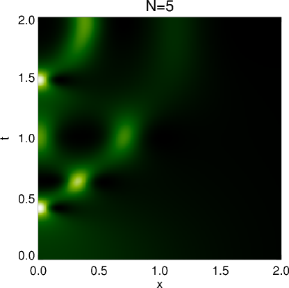
Figure 1. The square modulus of $\psi_{5}(x,t)$ plotted over a part of the positive quadrant of the $(x,t)$-plane.

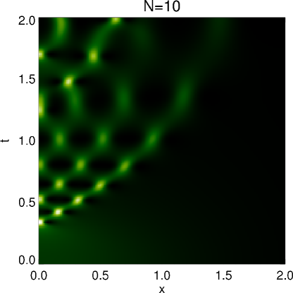
Figure 2. The square modulus of $\psi_{10}(x,t)$ plotted over a part of the positive quadrant of the $(x,t)$-plane.

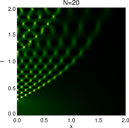
Figure 3. The square modulus of $\psi_{20}(x,t)$ plotted over a part of the positive quadrant of the $(x,t)$-plane.

Figure 4. The square modulus of $\psi_{40}(x,t)$ plotted over a part of the positive quadrant of the $(x,t)$-plane.

2.3. Phenomenology of the $N$-soliton for large $N$.

In each of Figures 1–4, the plotted solutions share some common features. After an initial period of smoothness, the solution changes over to a form with a central oscillatory region and quiescent tails. What is particularly striking in this sequence of figures is how the boundary between these two behaviors of the solution appears to become increasingly sharp as $N$ increases. This initial boundary curve is called the primary caustic. The solution up to and just beyond the primary caustic has been carefully studied in [10]. See also the discussion in § 4 below.

In Figure 3 and Figure 4, a second transition of solution behavior is clearly visible. It is this secondary caustic curve which is the main focus of this paper. As our subsequent analysis makes clear, this second phase transition is linked to the presence of the discrete soliton eigenvalues $\{\lambda_{N,k}\}\cup\{\lambda_{N,k}^{*}\}$, and the mechanism for this transition is different that of the transition across the primary caustic.

We note that Tovbis, Venakides, and Zhou [15] have studied the semiclassically scaled focusing nonlinear Schrödinger equation for a one-parameter family of special initial data. The forward-scattering procedure for this family [14] generates a reflection coefficent and — depending on the value of the parameter — some discrete soliton eigenvalues. (By contrast, recall that our initial data is reflectionless.) For those values of the parameter for which there are no discrete eigenvalues, they prove that the solution undergoes only a single phase transition and that there is no secondary caustic. When the value of the parameter is such that there are both solitons and reflection, they leave the possibility of a second phase transition as an open question.

3. Method of Asymptotic Analysis

3.1. Discrete Riemann-Hilbert problem.

For each fixed positive integer $N$, and for fixed real values of $x$ and $t$, consider solving the following problem: find a $2\times 2$ matrix ${\bf m}(\lambda;N,x,t)$ with entries that are rational functions of $\lambda$ such that

• The poles are all simple and are confined to the points $\{\lambda_{N,k}\}_{k=0}^{N-1}$ and $\{\lambda_{N,k}^{*}\}_{k=0}^{N-1}$, such that

  (23) $$\mathop{\text{Res}}_{\lambda_{N,k}}{\bf m}(\lambda;N,x,t)=\lim_{\lambda\rightarrow\lambda_{N,k}}{\bf m}(\lambda;N,x,t)\left[\begin{array}[]{cc}0&0\\ c_{N,k}(x,t)&0\end{array}\right]\,,$$

  and

  (24) $$\mathop{\text{Res}}_{\lambda_{N,k}^{*}}{\bf m}(\lambda;N,x,t)=\lim_{\lambda\rightarrow\lambda_{N,k}^{*}}{\bf m}(\lambda;N,x,t)\left[\begin{array}[]{cc}0&-c_{N,k}(x,t)^{*}\\ 0&0\end{array}\right]\,,$$

  hold for $k=0,\dots,N-1$, where $c_{N,k}(x,t):=c_{N,k}^{0}e^{2iQ(\lambda_{N,k};x,t)/\hbar_{N}}$, and,

  (25) $$c_{N,k}^{0}:=\frac{1}{\gamma_{N,k}}\frac{\displaystyle\prod_{n=0}^{N-1}\lambda_{N,k}-\lambda_{N,n}^{*}}{\displaystyle\mathop{\prod_{n=0}^{N-1}}_{n\neq k}\lambda_{N,k}-\lambda_{N,n}}\,,\hskip 14.45377ptQ(\lambda;x,t):=\lambda x+\lambda^{2}t\,.$$

• The matrix ${\bf m}(\lambda;N,x,t)$ is normalized so that

  (26) $$\lim_{\lambda\rightarrow\infty}{\bf m}(\lambda;N,x,t)=\mathbb{I}\,.$$

Then, the function defined in terms of ${\bf m}(\lambda;N,x,t)$ by the limit

(27) $$\psi_{N}(x,t):=2i\lim_{\lambda\rightarrow\infty}\lambda m_{12}(\lambda;N,x,t)$$

is the $N$-soliton solution of the semiclassically scaled focusing nonlinear Schrödinger equation.

This Riemann-Hilbert problem essentially encodes the linear equations introduced in § 2 describing the $N$-soliton, in a way that is conducive to asymptotic analysis in the limit $N\rightarrow\infty$. That the function $\psi_{N}(x,t)$ solves the semiclassically scaled focusing nonlinear Schrödinger equation (3) is easy to show. Indeed, let ${\bf n}(\lambda;N,x,t)={\bf m}(\lambda;N,x,t)e^{-iQ(\lambda;x,t)\sigma_{3}/\hbar_{N}}$. Then, it is easy to check that the residue conditions on ${\bf m}(\lambda;N,x,t)$ translate into analogous conditions on ${\bf n}(\lambda;N,x,t)$ that are independent of $x$ and $t$:

(28) $$\mathop{\text{Res}}_{\lambda_{N,k}}{\bf n}(\lambda;N,x,t)=\lim_{\lambda\rightarrow\lambda_{N,k}}{\bf n}(\lambda;N,x,t)\left[\begin{array}[]{cc}0&0\\ c_{N,k}^{0}&0\end{array}\right]\,,$$

and

(29) $$\mathop{\text{Res}}_{\lambda_{N,k}^{*}}{\bf n}(\lambda;N,x,t)=\lim_{\lambda\rightarrow\lambda_{N,k}^{*}}{\bf n}(\lambda;N,x,t)\left[\begin{array}[]{cc}0&-c_{N,k}^{0*}\\ 0&0\end{array}\right]\,.$$

It is easy to see that $\det({\bf n}(\lambda;N,x,t))\equiv 1$, because clearly the determinant is a meromorphic function, with possible simple poles only at the points $\{\lambda_{N,k}\}\cup\{\lambda_{N,k}^{*}\}$, that tends to one as $\lambda\rightarrow\infty$. But from the residue conditions it is easy to verify that $\det({\bf n}(\lambda;N,x,t))$ is regular at the possible poles, and so is an entire function tending to one at infinity that by Liouville’s Theorem must be constant. In particular, ${\bf n}(\lambda;N,x,t)$ is nonsingular for all $\lambda$, so it follows that $\partial_{x}{\bf n}(\lambda;N,x,t){\bf n}(\lambda;N,x,t)^{-1}$ and $\partial_{t}{\bf n}(\lambda;N,x,t){\bf n}(\lambda;N,x,t)^{-1}$ are both entire functions of $\lambda$. Moreover, they are polynomials in $\lambda$, as can be deduced from their growth at infinity. Indeed, ${\bf m}(\lambda;N,x,t)$ necessarily has an expansion

(30) $${\bf m}(\lambda;N,x,t)=\mathbb{I}+\sum_{p=1}^{\infty}\lambda^{-p}{\bf m}_{p}\,,\hskip 14.45377pt{\bf m}_{p}={\bf m}_{p}(N,x,t)\,,$$

which is uniformly convergent for $|\lambda|$ sufficiently large (larger than the modulus of any prescribed singularity of ${\bf m}(\lambda;N,x,t)$ is enough), and differentiable term-by-term with respect to $x$ and $t$. Therefore,

(31) $$\begin{array}[]{rcl}\displaystyle\partial_{x}{\bf n}(\lambda;N,x,t){\bf n}(\lambda;N,x,t)^{-1}&=&\displaystyle\partial_{x}\left[\left(\mathbb{I}+\lambda^{-1}{\bf m}_{1}+\lambda^{-2}{\bf m}_{2}+\cdots\right)e^{-iQ(\lambda;x,t)\sigma_{3}/\hbar_{N}}\right]\\ \\ &&\displaystyle\cdot e^{iQ(\lambda;x,t)\sigma_{3}/\hbar_{N}}\left(\mathbb{I}-\lambda^{-1}{\bf m}_{1}+\lambda^{-2}({\bf m}_{1}^{2}-{\bf m}_{2})+\cdots\right)\\ \\ &=&\displaystyle\left(-i\hbar_{N}^{-1}\lambda\sigma_{3}-i\hbar_{N}^{-1}{\bf m}_{1}\sigma_{3}+\cdots\right)\cdot(\mathbb{I}-\lambda^{-1}{\bf m}_{1}+\cdots)\\ \\ &=&\displaystyle-i\hbar_{N}^{-1}\left(\lambda\sigma_{3}+[{\bf m}_{1},\sigma_{3}]\right)\,.\end{array}$$

Similarly,

(32) $$\begin{array}[]{rcl}\displaystyle\partial_{t}{\bf n}(\lambda;N,x,t){\bf n}(\lambda;N,x,t)^{-1}&=&\displaystyle\partial_{t}\left[\left(\mathbb{I}+\lambda^{-1}{\bf m}_{1}+\lambda^{-2}{\bf m}_{2}+\cdots\right)e^{-iQ(\lambda;x,t)\sigma_{3}/\hbar_{N}}\right]\\ \\ &&\displaystyle\cdot e^{iQ(\lambda;x,t)\sigma_{3}/\hbar_{N}}\left(\mathbb{I}-\lambda^{-1}{\bf m}_{1}+\lambda^{-2}({\bf m}_{1}^{2}-{\bf m}_{2})+\cdots\right)\\ \\ &=&\displaystyle\left(-i\hbar_{N}^{-1}\lambda^{2}\sigma_{3}-i\hbar_{N}^{-1}\lambda{\bf m}_{1}\sigma_{3}-i\hbar_{N}^{-1}{\bf m}_{2}\sigma_{3}+\cdots\right)\\ \\ &&\displaystyle\cdot(\mathbb{I}-\lambda^{-1}{\bf m}_{1}+\lambda^{-2}({\bf m}_{1}^{2}-{\bf m}_{2})+\cdots)\\ \\ &=&\displaystyle-i\hbar_{N}^{-1}\left(\lambda^{2}\sigma_{3}+\lambda[{\bf m}_{1},\sigma_{3}]+[{\bf m}_{2},\sigma_{3}]-[{\bf m}_{1},\sigma_{3}]{\bf m}_{1}\right)\,.\end{array}$$

Consequently, ${\bf n}(\lambda;N,x,t)$ is a simultaneous fundamental solution matrix for general $\lambda$ of the linear differential equations

(33) $$\begin{array}[]{rcl}\displaystyle i\hbar_{N}\partial_{x}{\bf n}(\lambda;N,x,t)&=&\displaystyle\left(\lambda\sigma_{3}+[{\bf m}_{1},\sigma_{3}]\right){\bf n}(\lambda;N,x,t)\\ \\ \displaystyle i\hbar_{N}\partial_{t}{\bf n}(\lambda;N,x,t)&=&\displaystyle\left(\lambda^{2}\sigma_{3}+\lambda[{\bf m}_{1},\sigma_{3}]+[{\bf m}_{2},\sigma_{3}]-[{\bf m}_{1},\sigma_{3}]{\bf m}_{1}\right){\bf n}(\lambda;N,x,t)\,.\end{array}$$

The coefficient matrices therefore satisfy the zero-curvature compatibility condition

(34) $$\begin{array}[]{l}\displaystyle i\hbar_{N}\partial_{t}\left(\lambda\sigma_{3}+[{\bf m}_{1},\sigma_{3}]\right)-i\hbar_{N}\partial_{x}\left(\lambda^{2}\sigma_{3}+\lambda[{\bf m}_{1},\sigma_{3}]+[{\bf m}_{2},\sigma_{3}]-[{\bf m}_{1},\sigma_{3}]{\bf m}_{1}\right)\\ \\ \displaystyle\hskip 72.26999pt+\,\,\,[\lambda\sigma_{3}+[{\bf m}_{1},\sigma_{3}],\lambda^{2}\sigma_{3}+\lambda[{\bf m}_{1},\sigma_{3}]+[{\bf m}_{2},\sigma_{3}]-[{\bf m}_{1},\sigma_{3}]{\bf m}_{1}]=0\,.\end{array}$$

Separating out the coefficients of the powers of $\lambda$ we obtain two nontrivial equations:

(35) $$-i\hbar_{N}\partial_{x}[{\bf m}_{1},\sigma_{3}]-[[{\bf m}_{2},\sigma_{3}],\sigma_{3}]+[[{\bf m}_{1},\sigma_{3}]{\bf m}_{1},\sigma_{3}]=0\,,$$

and

(36) $$i\hbar_{N}\partial_{t}[{\bf m}_{1},\sigma_{3}]-i\hbar_{N}\partial_{x}\left([{\bf m}_{2},\sigma_{3}]-[{\bf m}_{1},\sigma_{3}]{\bf m}_{1}\right)+[[{\bf m}_{1},\sigma_{3}],[{\bf m}_{2},\sigma_{3}]]-[[{\bf m}_{1},\sigma_{3}],[{\bf m}_{1},\sigma_{3}]{\bf m}_{1}]=0\,.$$

Introducing the notation

(37) $${\bf A}={\bf A}^{D}+{\bf A}^{OD}\,,$$

for separating a $2\times 2$ matrix into its diagonal and off-diagonal parts, we have for any ${\bf A}$:

(38) $$[{\bf A},\sigma_{3}]=2{\bf A}^{OD}\sigma_{3}\,,$$

The first equation becomes

(39) $$-i\hbar_{N}\partial_{x}{\bf m}_{1}^{OD}\sigma_{3}-2{\bf m}_{2}^{OD}+2{\bf m}_{1}^{OD}{\bf m}_{1}^{D}=0\,,$$

which is purely off-diagonal, while the second equation has both diagonal parts:

(40) $$i\hbar_{N}\partial_{x}({\bf m}_{1}^{OD}\sigma_{3}{\bf m}_{1}^{OD})+2[{\bf m}_{1}^{OD}\sigma_{3},{\bf m}_{2}^{OD}\sigma_{3}]-2[{\bf m}_{1}^{OD}\sigma_{3},{\bf m}_{1}^{OD}\sigma_{3}{\bf m}_{1}^{D}]=0\,,$$

and off-diagonal parts:

(41) $$i\hbar_{N}\partial_{t}({\bf m}_{1}^{OD}\sigma_{3})-\frac{iA}{M}\partial_{x}({\bf m}_{2}^{OD}\sigma_{3})+\frac{iA}{M}\partial_{x}({\bf m}_{1}^{OD}{\bf m}_{1}^{D}\sigma_{3})-2[{\bf m}_{1}^{OD}\sigma_{3},{\bf m}_{1}^{OD}\sigma_{3}{\bf m}_{1}^{OD}]=0\,.$$

Eliminating ${\bf m}_{2}^{OD}$ using the first equation, the off-diagonal part of the second equation becomes:

(42) $$i\hbar_{N}\sigma_{3}\partial_{t}{\bf m}_{1}^{OD}+\frac{\hbar_{N}^{2}}{2}\partial_{x}^{2}{\bf m}_{1}^{OD}-4{\bf m}_{1}^{OD3}=0\,.$$

In other words, if we introduce notation for the off-diagonal elements of ${\bf m}_{1}$ as follows,

(43) $${\bf m}_{1}^{OD}=\left[\begin{array}[]{cc}0&q\\ r&0\end{array}\right]\,,$$

then $q$ and $r$ satisfy a coupled system of partial differential equations:

(44) $$i\hbar_{N}\partial_{t}q+\frac{\hbar_{N}^{2}}{2}\partial_{x}^{2}q-4rq^{2}=0\,,\hskip 14.45377pt-i\hbar_{N}\partial_{t}r+\frac{\hbar_{N}^{2}}{2}\partial_{x}^{2}r-4qr^{2}=0\,.$$

If for all $x$ and $t$ we have $r=-q^{*}$, then these become the focusing nonlinear Schrödinger equation

(45) $$i\hbar_{N}\partial_{t}\psi+\frac{\hbar_{N}^{2}}{2}\partial_{x}^{2}\psi+|\psi|^{2}\psi=0\,,\hskip 14.45377pt\psi=2iq=-2ir^{*}\,.$$

Therefore, to complete the proof, it remains only to show that indeed $r=-q^{*}$. To do this we consider along with the solution ${\bf m}(\lambda;N,x,t)$ of the discrete Riemann-Hilbert problem the corresponding matrix $\tilde{\bf m}(\lambda;N,x,t):=\sigma_{2}{\bf m}(\lambda^{*};N,x,t)^{*}\sigma_{2}$, where the star denotes componentwise complex conjugation. Clearly $\tilde{\bf m}(\lambda;N,x,t)$ is analytic in $\lambda$ with simple poles at $\{\lambda_{N,k}\}\cup\{\lambda_{N,k}^{*}\}$ (because the pole set is complex-conjugate invariant) and tends to the identity as $\lambda\rightarrow\infty$ (because $\sigma_{2}^{2}=\mathbb{I}$). Furthermore,

(46) $$\begin{array}[]{rcl}\displaystyle\mathop{\text{Res}}_{\lambda_{N,k}}\tilde{\bf m}(\lambda;N,x,t)&=&\displaystyle\sigma_{2}\left(\mathop{\text{Res}}_{\lambda_{N,k}^{*}}{\bf m}(\lambda;N,x,t)\right)^{*}\sigma_{2}\\ \\ &=&\displaystyle\sigma_{2}\left(\lim_{\lambda\rightarrow\lambda_{N,k}^{*}}{\bf m}(\lambda;N,x,t)\left[\begin{array}[]{cc}0&-c_{N,k}(x,t)^{*}\\ 0&0\end{array}\right]\right)^{*}\sigma_{2}\\ \\ &=&\displaystyle\lim_{\lambda\rightarrow\lambda_{N,k}}\tilde{\bf m}(\lambda;N,x,t)\sigma_{2}\left[\begin{array}[]{cc}0&-c_{N,k}(x,t)\\ 0&0\end{array}\right]\sigma_{2}\\ \\ &=&\displaystyle\lim_{\lambda\rightarrow\lambda_{N,k}}\tilde{\bf m}(\lambda;N,x,t)\left[\begin{array}[]{cc}0&0\\ c_{N,k}(x,t)&0\end{array}\right]\,.\end{array}$$

By a similar calculation,

(47) $$\mathop{\text{Res}}_{\lambda_{N,k}^{*}}\tilde{\bf m}(\lambda;N,x,t)=\lim_{\lambda\rightarrow\lambda_{N,k}^{*}}\tilde{\bf m}(\lambda;N,x,t)\left[\begin{array}[]{cc}0&-c_{N,k}(x,t)^{*}\\ 0&0\end{array}\right]\,.$$

It follows that ${\bf m}(\lambda;N,x,t)\tilde{\bf m}(\lambda;N,x,t)^{-1}$ is an entire function of $\lambda$ that tends to the identity matrix as $\lambda\rightarrow\infty$. By Liouville’s Theorem, we thus have $\tilde{\bf m}(\lambda;N,x,t)\equiv{\bf m}(\lambda;N,x,t)$. Expanding both sides of this identity near $\lambda=\infty$, we get

(48) $$\mathbb{I}+\lambda^{-1}{\bf m}_{1}=\mathbb{I}+\lambda^{-1}\sigma_{2}{\bf m}_{1}^{*}\sigma_{2}+O(\lambda^{-2})\,,$$

so in particular,

(49) $${\bf m}_{1}^{OD}=\sigma_{2}{\bf m}_{1}^{OD*}\sigma_{2}\,,$$

which gives $r=-q^{*}$.

That the function $\psi_{N}(x,t)$ satisfies $\psi_{N}(x,0)=A\,\text{sech}(x)$ for all $N$ is more difficult to show by studying properties of the matrix ${\bf m}(\lambda;N,x,t)$. In general, this follows from solving the corresponding direct-scattering problem which was done with the help of hypergeometric functions by Satsuma and Yajima [13]. Here we illustrate the corresponding inverse-scattering calculation in the most tractable case of $N=1$. When $N=1$, ${\bf m}(\lambda;1,x,0)$ may be sought in the form

(50) $${\bf m}(\lambda;1,x,0)=\left[\begin{array}[]{cc}\displaystyle\frac{\lambda+\alpha_{11}(x)}{\lambda-iA/2}&\displaystyle\frac{\alpha_{12}(x)}{\lambda+iA/2}\\ \\ \displaystyle\frac{\alpha_{21}(x)}{\lambda-iA/2}&\displaystyle\frac{\lambda+\alpha_{22}(x)}{\lambda+iA/2}\end{array}\right]\,.$$

The residue relations then say that

(51) $$\begin{array}[]{rcl}\displaystyle iA/2+\alpha_{11}(x)&=&\displaystyle-iAe^{-x}\cdot\frac{\alpha_{12}(x)}{iA}\,,\\ \\ \displaystyle\alpha_{21}(x)&=&\displaystyle-iAe^{-x}\cdot\frac{iA/2+\alpha_{22}(x)}{iA}\,,\\ \\ \displaystyle\alpha_{12}(x)&=&\displaystyle-iAe^{-x}\cdot\frac{iA/2-\alpha_{11}(x)}{iA}\,,\\ \\ \displaystyle-iA/2+\alpha_{22}(x)&=&\displaystyle-iAe^{-x}\cdot\frac{-\alpha_{21}(x)}{iA}\,,\end{array}$$

It follows that $\alpha_{12}(x)=-iA\,\text{sech}(x)/2$, from which we indeed find that $\psi_{1}(x,0)=A\,\text{sech}(x)$.

3.2. First modification: removal of poles.

3.2.1. Interpolation of residues.

In the following, to keep the notation as simple as possible, we suppress the parametric dependence on $N$, $x$, and $t$. We first modify the matrix unknown ${\bf m}(\lambda):={\bf m}(\lambda;N,x,t)$ by multiplication on the right by an explicit matrix factor which differs from the identity matrix in the regions $D_{1}$, $D_{-1}$, and their complex conjugates, as shown in Figure 5.

Figure 5. The regions $D_{1}$ and $D_{-1}$ in the upper half-plane, and the oriented boundary arcs $K_{-1}$, $K_{0}$, and $K_{1}$. The $N$ soliton eigenvalues $\{\lambda_{N,k}\}_{k=0}^{N-1}$ and the imaginary interval $[0,iA]$ in which they accumulate as $N\rightarrow\infty$ are shown in red. The number $\epsilon>0$ will be taken later to be sufficiently small, but independent of $N$.

Let $K_{0}$ denote the common boundary arc of $D_{1}$ and $D_{-1}$ oriented in the direction away from the origin. Let $K_{1}$ denote the remaining part of the boundary of $D_{1}$ lying in the open upper half-plane, oriented in the direction toward $\lambda=\epsilon$. Let $K_{-1}$ denote the remaining part of the boundary of $D_{-1}$ lying in the open upper half-plane, oriented in the direction toward $\lambda=-\epsilon$. We will call the point where the three contour arcs $K_{j}$ meet $\lambda_{0}$.

Note that the region $D_{-1}$ contains the soliton eigenvalues $\{\lambda_{N,k}\}_{k=0}^{N-1}$ for all $N$. The region $D_{1}$ is needed for a technical reason; with its help we will be able to ultimately remove some jump discontinuities from the neighborhood of $\lambda=0$. We set

(52) $${\bf M}(\lambda):={\bf m}(\lambda)\left[\begin{array}[]{cc}1&0\\ -iP(\lambda)e^{[2iQ(\lambda)+i\theta^{0}(\lambda)]/\hbar}&1\end{array}\right]\,,\hskip 14.45377pt\text{for $\lambda\in D_{1}$,}$$

(53) $${\bf M}(\lambda):={\bf m}(\lambda)\left[\begin{array}[]{cc}1&0\\ iP(\lambda)e^{[2iQ(\lambda)-i\theta^{0}(\lambda)]/\hbar}&1\end{array}\right]\,,\hskip 14.45377pt\text{for $\lambda\in D_{-1}$,}$$

For all $\lambda$ in the upper half-plane outside the closure of $D_{1}\cup D_{-1}$, we set ${\bf M}(\lambda)={\bf m}(\lambda)$. For $\lambda$ in the lower half-plane, we define ${\bf M}(\lambda):=\sigma_{2}{\bf M}(\lambda^{*})^{*}\sigma_{2}$, where the star denotes componentwise complex-conjugation. Here, we are using the notation

(54) $$P(\lambda):=\prod_{k=0}^{N-1}\frac{\lambda-\lambda_{N,k}^{*}}{\lambda-\lambda_{N,k}}\,,$$

and

(55) $$\theta^{0}(\lambda):=i\pi\lambda+\pi A\,,$$

and, $\hbar=\hbar_{N}$. It is easy to see that the matrix ${\bf M}(\lambda)$ is holomorphic at the soliton eigenvalues $\lambda=\lambda_{N,k}$ where ${\bf m}(\lambda)$ has its poles in the upper half-plane.

3.2.2. Aside: even symmetry of $\psi_{N}(x,t)$ in $x$ and the formal continuum limit.

Since ${\bf M}(\lambda)={\bf m}(\lambda)$ in a neighborhood of $\lambda=\infty$, the $N$-soliton is equivalently defined by the formula

(56) $$\psi_{N}(x,t)=2i\lim_{\lambda\rightarrow\infty}\lambda M_{12}(\lambda)\,.$$

From the conditions determining ${\bf M}(\lambda)$ is is easy to show that $\psi_{N}(x,t)$ is, for each $N$ and each $t$, an even function of $x$. For this purpose, we may suppose without any modification of $\psi_{N}(x,t)$ that $\epsilon=0$, that $D_{1}=\emptyset$, and that $D_{-1}$ is symmetric about the imaginary axis. We also temporarily re-introduce the explicit parametric dependence on $x$, and suppose that $D_{-1}$ is fixed as $x\in\mathbb{R}$ varies. Then the matrix ${\bf M}(-\lambda;x)$ has the same domain of analyticity as ${\bf M}(\lambda;x)$, and therefore we may compare ${\bf M}(\lambda;x)$ with the matrix ${\bf M}^{\sharp}(\lambda;x)$ defined by setting

(57) $${\bf M}^{\sharp}(\lambda;x):=\sigma_{3}{\bf M}(-\lambda;x)\sigma_{3}\left[\begin{array}[]{cc}0&ie^{[2i(\lambda x-\lambda^{2}t)+i\theta^{0}(\lambda)]/\hbar}\\ ie^{-[2i(\lambda x-\lambda^{2}t)+i\theta^{0}(\lambda)]/\hbar}&P(\lambda)^{-1}\end{array}\right]\,,\hskip 14.45377pt\lambda\in D_{-1}\,,$$

while elsewhere in the upper half-plane we set

(58) $${\bf M}^{\sharp}(\lambda;x):=\sigma_{3}{\bf M}(-\lambda;x)\sigma_{3}P(\lambda)^{\sigma_{3}}\,,$$

and then we define ${\bf M}^{\sharp}(\lambda;x)$ for $\lambda$ in the lower half-plane by setting ${\bf M}^{\sharp}(\lambda;x):=\sigma_{2}{\bf M}^{\sharp}(\lambda^{*};x)^{*}\sigma_{2}$ for $\Im(\lambda)<0$. Note that because the zeros of $P(\lambda)$ are confined to $D_{-1}^{*}$ while the poles are confined to $D_{-1}$, this defines ${\bf M}^{\sharp}(\lambda;x)$ as a sectionally holomorphic function of $\lambda$ with the same ($x$-independent) domain of analyticity as ${\bf M}(\lambda;x)$.

Now, if we use a subscript “$+$” (respectively “$-$”) to denote a boundary value taken on the boundary of $D_{-1}$ from inside (respectively outside), then it is an easy exercise to check that

(59) $${\bf M}^{\sharp}_{-}(\lambda;x)^{-1}{\bf M}^{\sharp}_{+}(\lambda;x)={\bf M}_{-}(\lambda;-x)^{-1}{\bf M}_{+}(\lambda;-x)\,,\hskip 14.45377pt\text{for $x\in\mathbb{R}$ and $\lambda\in\partial D_{-1}\cup\partial D_{-1}^{*}$\,.}$$

Also, since $P(\lambda)\rightarrow 1$ as $\lambda\rightarrow\infty$, it follows that ${\bf M}^{\sharp}(\lambda;x)\rightarrow\mathbb{I}$ as $\lambda\rightarrow\infty$ for each $x\in\mathbb{R}$. By Liouville’s Theorem, which assures the uniqueness of ${\bf M}(\lambda;x)$ given the jump condition across $\partial D_{-1}\cup\partial D_{-1}^{*}$ and the normalization condition at $\lambda=\infty$, it follows that

(60) $${\bf M}^{\sharp}(\lambda;x)={\bf M}(\lambda;-x)\,.$$

Using this relation, we clearly have that

(61) $$2i\lim_{\lambda\rightarrow\infty}\lambda{M}^{\sharp}_{12}(\lambda;x)=2i\lim_{\lambda\rightarrow\infty}\lambda M_{12}(\lambda;-x)=\psi_{N}(-x,t)\,,$$

where the last equality follows from (56). On the other hand, directly from the definition (58) valid for sufficiently large $|\lambda|$, we may use the fact that $P(\lambda)\rightarrow 1$ as $\lambda\rightarrow\infty$ to conclude that

(62) $$2i\lim_{\lambda\rightarrow\infty}\lambda{M}^{\sharp}_{12}(\lambda;x)=-2i\lim_{\lambda\rightarrow\infty}\lambda M_{12}(-\lambda;x)=2i\lim_{\mu\rightarrow\infty}\mu M_{12}(\mu;x)=\psi_{N}(x,t)\,.$$

Therefore we learn that $\psi_{N}(-x,t)=\psi_{N}(x,t)$ holds for all real $x$, so the $N$-soliton is an even function of $x$ for each $t$. Therefore, in all remaining calculations in this paper we will suppose without loss of generality that $x\geq 0$. (Since from (3) we see that time reversal is equivalent to complex conjugation of $\psi_{N}(x,t)$ because $\psi_{N}(x,0)$ is real, we will also assume that $t\geq 0$.) These choices lead to certain asymmetries in the complex plane as already apparent in Figure 5; for a discussion of how choice of signs of $x$ and $t$ relates to the parity of certain structures in the complex spectral plane that are introduced to aid in asymptotic analysis, see [10].

The even symmetry of $\psi_{N}(x,t)$ in $x$ is not an earth-shattering result, of course, but what is interesting is that the same argument fails completely if a natural continuum limit related to the limit $N\rightarrow\infty$ is introduced on an ad hoc basis. Indeed, it is natural to consider replacing the product $P(\lambda)$ by a formal continuum limit by “condensing the poles” as follows: define

(63) $$\tilde{P}(\lambda):=\exp\left(\frac{1}{\hbar}\left[i\int_{0}^{iA}\log(-i(\lambda-\eta))\,d\eta-i\int_{-iA}^{0}\log(-i(\lambda-\eta))\,d\eta\right]\right)\,,$$

which may be viewed as coming from interpreting the sums in the exact formula

(64) $$P(\lambda)=\exp\left(\frac{1}{\hbar}\left[\sum_{k=0}^{N-1}\log(\lambda-\lambda_{N,k}^{*})\hbar-\sum_{k=0}^{N-1}\log(\lambda-\lambda_{N,k})\hbar\right]\right)$$

as Riemann sums and passing to the natural integral limit for $\lambda$ fixed. The function $\tilde{P}(\lambda)$ is analytic for $\lambda\in\mathbb{C}\setminus[-iA,iA]$, and where $P(\lambda)$ has accumulating poles and zeros, $\tilde{P}(\lambda)$ has a logarithmic branch cut. Then, while ${\bf M}(\lambda;x)$ is defined as being a matrix with the symmetry ${\bf M}(\lambda;x)=\sigma_{2}{\bf M}(\lambda^{*};x)^{*}\sigma_{2}$ that satisfies the normalization condition ${\bf M}(\lambda;x)\rightarrow\mathbb{I}$ as $\lambda\rightarrow\infty$ and is analytic except on $\partial D_{-1}\cup\partial D_{-1}^{*}$ along which it takes continuous boundary values related by

(65) $${\bf M}_{+}(\lambda;x)={\bf M}_{-}(\lambda;x)\left[\begin{array}[]{cc}1&0\\ iP(\lambda)e^{[2i(\lambda x+\lambda^{2}t)-i\theta^{0}(\lambda)]/\hbar}&1\end{array}\right]\,,\hskip 14.45377pt\lambda\in\partial D_{-1}\,,$$

we may define a matrix $\tilde{\bf M}(\lambda)$ that satisfies exactly the same conditions as ${\bf M}(\lambda)$ but with $P(\lambda)$ replaced by $\tilde{P}(\lambda)$ in the jump condition. It is a direct matter to show that like $\psi_{N}(x,t)$, the function defined by

(66) $$\tilde{\psi}_{N}(x,t):=2i\lim_{\lambda\rightarrow\infty}\lambda\tilde{M}_{12}(\lambda;x)$$

is also a solution of the semiclassically scaled focusing nonlinear Schrödinger equation (3) (virtually the same arguments apply as was used to prove this about $\psi_{N}(x,t)$). However, whether $\tilde{\psi}_{N}(x,t)$ is an even function of $x$ is in our opinion an open question. Indeed, if we try to mimic the above proof of evenness of $\psi_{N}(x,t)$, we would be inclined to try to define a matrix $\tilde{\bf M}^{\sharp}(\lambda;x)$ starting from $\tilde{\bf M}(\lambda;x)$ by formulae analogous to (57) and (58), but with $P(\lambda)$ replaced everywhere by $\tilde{P}(\lambda)$. Comparing $\tilde{\bf M}^{\sharp}(\lambda;x)$ with $\tilde{\bf M}(\lambda;-x)$ then becomes a problem, because while $\tilde{\bf M}(\lambda;-x)$ is analytic in $D_{-1}\cup D_{-1}^{*}$, the matrix $\tilde{\bf M}^{\sharp}(\lambda;x)$ has a jump discontinuity across the segment $[-iA,iA]$. Thus, in stark contrast with (60) we have

(67) $$\tilde{\bf M}^{\sharp}(\lambda;x)\neq\tilde{\bf M}(\lambda;-x)\,,$$

and we cannot conclude (by a completely analogous proof, anyway) any evenness of $\tilde{\psi}(x,t)$.

The possibility that $\tilde{\psi}_{N}(x,t)$ may not be an even function of $x$ while $\psi_{N}(x,t)$ most certainly is even casts some doubt on the prospect that $\tilde{\psi}_{N}(x,t)$ might be a good approximation to $\psi_{N}(x,t)$. As it is $\tilde{\psi}_{N}(x,t)$ that is related to the solution of the “continuum-limit” Riemann-Hilbert problem for a matrix $\tilde{\bf P}(\lambda)$ to be introduced in § 3.8, we have some reason to suspect at this point that without careful accounting of the errors introduced by making the ad hoc substitution $P(\lambda)\rightarrow\tilde{P}(\lambda)$, a study of the “condensed-pole” problem may not be relevant at all to the asymptotic analysis of the $N$-soliton $\psi_{N}(x,t)$, at least for certain $x$ and $t$. We will give evidence in this paper that such suspicion is entirely justifiable.

3.3. Second modification: introduction of $g$-function.

Suppose that $g(\lambda)$ is a function analytic for $\lambda\in\mathbb{C}\setminus(K_{-1}\cup K_{0}\cup K_{-1}^{*}\cup K_{0}^{*})$ that satisfies the symmetry condition

(68) $$g(\lambda)+g(\lambda^{*})^{*}=0\,,$$

and $g(\lambda)\rightarrow 0$ as $\lambda\rightarrow\infty$. Note that in particular $g(\lambda)$ is analytic in the real intervals $(-\epsilon,0)$ and $(0,\epsilon)$. We change variables again to a matrix function ${\bf N}(\lambda)$ by setting

(69) $${\bf N}(\lambda):={\bf M}(\lambda)e^{-g(\lambda)\sigma_{3}/\hbar}\,.$$

Letting the subscript “$+$” (respectively “$-$”) denote a boundary value taken on one of the contours $K_{j}$ from the left (respectively right) according to its orientation, we deduce from our definitions and the continuity of ${\bf m}(\lambda)$ across each of these contours that the following “jump relations” hold:

(70) $${\bf N}_{+}(\lambda)={\bf N}_{-}(\lambda)\left[\begin{array}[]{cc}e^{-[g_{+}(\lambda)-g_{-}(\lambda)]/\hbar}&0\\ iP(\lambda)e^{[2iQ(\lambda)-i\theta^{0}(\lambda)-g_{+}(\lambda)-g_{-}(\lambda)]/\hbar}&e^{[g_{+}(\lambda)-g_{-}(\lambda)]/\hbar}\end{array}\right]\,,\hskip 14.45377pt\lambda\in K_{-1}\,,$$

(71) $${\bf N}_{+}(\lambda)={\bf N}_{-}(\lambda)\left[\begin{array}[]{cc}1&0\\ iP(\lambda)e^{[2iQ(\lambda)+i\theta^{0}(\lambda)-2g(\lambda)]/\hbar}&1\end{array}\right]\,,\hskip 14.45377pt\lambda\in K_{1}\,,$$

(72) $${\bf N}_{+}(\lambda)={\bf N}_{-}(\lambda)\left[\begin{array}[]{cc}e^{-[g_{+}(\lambda)-g_{-}(\lambda)]/\hbar}&0\\ 2iP(\lambda)\cos(\theta^{0}(\lambda)/\hbar)e^{[2iQ(\lambda)-g_{+}(\lambda)-g_{-}(\lambda)]/\hbar}&e^{[g_{+}(\lambda)-g_{-}(\lambda)]/\hbar}\end{array}\right]\,,\hskip 14.45377pt\lambda\in K_{0}\,.$$

The jump relations holding on the conjugate contours in the lower half-plane follow from the symmetry ${\bf N}(\lambda^{*})=\sigma_{2}{\bf N}(\lambda)^{*}\sigma_{2}$. Finally, there are also jump discontinuities across the real intervals $(-\epsilon,0)$ and $(0,\epsilon)$, both of which we assign an orientation from left to right. Using the above symmetry relation along with the facts (holding for $x$ and $t$ real and $\hbar=A/N$ with $N\in\mathbb{Z}$):

(73) $$P(\lambda^{*})^{*}=P(\lambda)^{-1}\,,\hskip 14.45377ptQ(\lambda^{*})^{*}=Q(\lambda)\,,\hskip 14.45377pt\theta^{0}(\lambda^{*})^{*}=-\theta^{0}(\lambda)+2\pi\hbar N\,,$$

we find that

(74) $${\bf N}_{+}(\lambda)={\bf N}_{-}(\lambda)\left[\begin{array}[]{cc}1+e^{-2i\theta_{0}(\lambda)/\hbar}&-iP(\lambda)^{-1}e^{[-2iQ(\lambda)-i\theta^{0}(\lambda)+2g(\lambda)]/\hbar}\\ iP(\lambda)e^{[2iQ(\lambda)-i\theta^{0}(\lambda)-2g(\lambda)]/\hbar}&1\end{array}\right]\,,\hskip 14.45377pt\lambda\in(-\epsilon,0)\,,$$

(75) $${\bf N}_{+}(\lambda)={\bf N}_{-}(\lambda)\left[\begin{array}[]{cc}1+e^{2i\theta_{0}(\lambda)/\hbar}&iP(\lambda)^{-1}e^{[-2iQ(\lambda)+i\theta^{0}(\lambda)+2g(\lambda)]/\hbar}\\ -iP(\lambda)e^{[2iQ(\lambda)+i\theta^{0}(\lambda)-2g(\lambda)]/\hbar}&1\end{array}\right]\,,\hskip 14.45377pt\lambda\in(0,\epsilon)\,.$$

Let $C$ denote a simple contour lying in $D_{-1}$ starting from the origin and terminating at $\lambda=iA$. There is a unique function $L(\lambda)$ with the properties that (i) it is analytic for $\lambda\in\mathbb{C}\setminus(C\cup C^{*})$, (ii) it takes continuous boundary values on each side of the contour $C\cup C^{*}$ satisfying

(76) $$L_{+}(\lambda)-L_{-}(\lambda)=\left\{\begin{array}[]{ll}-2i\theta^{0}(\lambda)\,,&\hskip 14.45377pt\text{for $\lambda\in C$,}\\ -2i\theta^{0}(\lambda^{*})^{*}\,,&\hskip 14.45377pt\text{for $\lambda\in C^{*}$,}\end{array}\right.$$

where $L_{+}(\lambda)$ (respectively $L_{-}(\lambda)$) refers to the boundary value taken on $C\cup C^{*}$ from the left (respectively right) as it is traversed from $-iA$ to $iA$, and (iii) it is normalized so that $L(\lambda)$ tends to zero as $\lambda\rightarrow\infty$. Indeed, the function $L(\lambda)$ is easily seen to be unique from these conditions (by Liouville’s theorem and continuity of the boundary values as is compatible with the conditions (76)) and we will give an explicit construction later (see (102)–(107)). The function $L(\lambda)$ enjoys the following symmetry property:

(77) $$L(\lambda)+L(\lambda^{*})^{*}=0\,.$$

Related to $L(\lambda)$ is another function $\overline{L}(\lambda)$ defined as follows. Let $C_{\infty}$ denote an infinite simple contour in the upper half-plane emanating from $\lambda=iA$ and tending to infinity in the upper half-plane, avoiding the domain $D_{1}$. Note that the union of contours $C\cup C_{\infty}\cup C^{*}\cup C_{\infty}^{*}$ divides the complex plane in half. We say that the left (right) half-plane according to $C\cup C_{\infty}\cup C^{*}\cup C_{\infty}^{*}$ is the half containing the negative (positive) real axis. For $\Im(\lambda)>0$ we then define

(78) $$\overline{L}(\lambda):=\left\{\begin{array}[]{ll}L(\lambda)+i\theta^{0}(\lambda)\,,&\hskip 14.45377pt\text{for $\lambda$ in the left half-plane according to $C\cup C_{\infty}\cup C^{*}\cup C_{\infty}^{*}$,}\\ L(\lambda)-i\theta^{0}(\lambda)\,,&\hskip 14.45377pt\text{for $\lambda$ in the right half-plane according to $C\cup C_{\infty}\cup C^{*}\cup C_{\infty}^{*}$.}\end{array}\right.$$

We note from (76) that $\overline{L}(\lambda)$ extends continuously to $C$ and thus may be viewed as a function analytic for $\lambda\in\mathbb{C}_{+}\setminus C_{\infty}$, where $\mathbb{C}_{+}$ denotes the upper half-plane. We introduce the notation

(79) $$T(\lambda):=2e^{-\overline{L}(\lambda)/\hbar}P(\lambda)\cos(\theta^{0}(\lambda)/\hbar)\,.$$

so the jump relation holding on $K_{0}$ may be equivalently written in the form

(80) $${\bf N}_{+}(\lambda)={\bf N}_{-}(\lambda)\left[\begin{array}[]{cc}e^{-[g_{+}(\lambda)-g_{-}(\lambda)]/\hbar}&0\\ iT(\lambda)e^{[2iQ(\lambda)+\overline{L}(\lambda)-g_{+}(\lambda)-g_{-}(\lambda)]/\hbar}&e^{[g_{+}(\lambda)-g_{-}(\lambda)]/\hbar}\end{array}\right]\,,\hskip 14.45377pt\lambda\in K_{0}\,.$$

The jump matrix in (80) can be factored as follows:

(81) $$\begin{array}[]{l}\displaystyle\left[\begin{array}[]{cc}e^{-[g_{+}(\lambda)-g_{-}(\lambda)]/\hbar}&0\\ iT(\lambda)e^{[2iQ(\lambda)+\overline{L}(\lambda)-g_{+}(\lambda)-g_{-}(\lambda)]/\hbar}&e^{[g_{+}(\lambda)-g_{-}(\lambda)]/\hbar}\end{array}\right]=\\ \\ \displaystyle\hskip 36.135pt\left[\begin{array}[]{cc}T(\lambda)^{-1/2}&-iT(\lambda)^{-1/2}e^{[-2iQ(\lambda)-\overline{L}(\lambda)+2g_{-}(\lambda)]/\hbar}\\ 0&T(\lambda)^{1/2}\end{array}\right]\times\\ \\ \displaystyle\hskip 36.135pt\left[\begin{array}[]{cc}0&ie^{[-2iQ(\lambda)-\overline{L}(\lambda)+g_{+}(\lambda)+g_{-}(\lambda)]/\hbar}\\ ie^{[2iQ(\lambda)+\overline{L}(\lambda)-g_{+}(\lambda)-g_{-}(\lambda)]/\hbar}&0\end{array}\right]\times\\ \\ \displaystyle\hskip 36.135pt\left[\begin{array}[]{cc}T(\lambda)^{1/2}&-iT(\lambda)^{-1/2}e^{[-2iQ(\lambda)-\overline{L}(\lambda)+2g_{+}(\lambda)]/\hbar}\\ 0&T(\lambda)^{-1/2}\end{array}\right]\,.\end{array}$$

Such a factorization makes sense because we will see later (in § 3.7) that $T(\lambda)\rightarrow 1$ as $N\rightarrow\infty$, so the fractional powers are well-defined for large enough $N$ as having similar asymptotics, converging to $1$ as $N\rightarrow\infty$. The left-most (respectively right-most) matrix factor is the boundary value on $K_{0}$ taken by a function analytic on the “minus” (respectively “plus”) side of $K_{0}$. Let $K_{L}$ denote a contour arc in $D_{-1}$ connecting the point $\lambda_{0}$ with the point $\lambda=-\epsilon$, and oriented in the direction away from $\lambda_{0}$. Let $D_{L}$ denote the region enclosed by $K_{0}$, $K_{L}$, and the interval $[-\epsilon,0]$. We introduce a new unknown ${\bf O}(\lambda)$ based on the above factorization as follows:

(82) $${\bf O}(\lambda):={\bf N}(\lambda)\left[\begin{array}[]{cc}T(\lambda)^{-1/2}&-iT(\lambda)^{-1/2}e^{[-2iQ(\lambda)-\overline{L}(\lambda)+2g(\lambda)]/\hbar}\\ 0&T(\lambda)^{1/2}\end{array}\right]\,,\hskip 14.45377pt\lambda\in D_{1}\,,$$

(83) $${\bf O}(\lambda):={\bf N}(\lambda)\left[\begin{array}[]{cc}T(\lambda)^{-1/2}&iT(\lambda)^{-1/2}e^{[-2iQ(\lambda)-\overline{L}(\lambda)+2g(\lambda)]/\hbar}\\ 0&T(\lambda)^{1/2}\end{array}\right]\,,\hskip 14.45377pt\lambda\in D_{L}\,,$$

and elsewhere in the upper half-plane we set ${\bf O}(\lambda):={\bf N}(\lambda)$. For $\lambda$ in the lower half-plane, we define ${\bf O}(\lambda)$ so as to preserve the symmetry ${\bf O}(\lambda^{*})=\sigma_{2}{\bf O}(\lambda)^{*}\sigma_{2}$.

Proposition 1.

The matrix ${\bf O}(\lambda)$ has no jump discontinuity across the real intervals $(-\epsilon,0)$ or $(0,\epsilon)$, and thus may be viewed as an analytic function for $\lambda\in\mathbb{C}\setminus(K_{-1}\cup K_{0}\cup K_{L}\cup K_{1}\cup K_{-1}^{*}\cup K_{0}^{*}\cup K_{L}^{*}\cup K_{1}^{*})$ that takes continuous boundary values from each region where it is analytic.

Proof.

The boundary value taken by ${\bf O}(\lambda)$ on $(0,\epsilon)$ from the upper half-plane is

(84) $${\bf O}_{+}(\lambda)={\bf N}_{+}(\lambda)\left[\begin{array}[]{cc}T(\lambda)^{-1/2}&-iT(\lambda)^{-1/2}e^{[-2iQ(\lambda)-L(\lambda)+i\theta^{0}(\lambda)+2g(\lambda)]/\hbar}\\ 0&T(\lambda)^{-1/2}\cdot P(\lambda)e^{[-L(\lambda)+i\theta^{0}(\lambda)]/\hbar}(e^{i\theta^{0}(\lambda)/\hbar}+e^{-i\theta^{0}(\lambda)/\hbar})\end{array}\right]\,,$$

which follows from (82), where we used the fact that $(0,\epsilon)$ is in the right half-plane according to $C\cup C_{\infty}\cup C^{*}\cup C_{\infty}^{*}$ to write $\overline{L}(\lambda)$ in terms of $L(\lambda)$ with the help of (78). Here all of the quantities in the exponent are analytic functions on $(0,\epsilon)$, and $T(\lambda)^{-1/2}$ is interpreted in the sense of its boundary value taken on $(0,\epsilon)$ from the upper half-plane. From the conjugation symmetry relations satisfied by ${\bf O}(\lambda)$ and ${\bf N}(\lambda)$, it then follows that the boundary value taken by ${\bf O}(\lambda)$ on $(0,\epsilon)$ from the lower half-plane is

(85) $${\bf O}_{-}(\lambda)={\bf N}_{-}(\lambda)\left[\begin{array}[]{cc}(T(\lambda^{*})^{*})^{-1/2}\cdot P(\lambda)^{-1}e^{[L(\lambda)+i\theta^{0}(\lambda)]/\hbar}(e^{i\theta^{0}(\lambda)/\hbar}+e^{-i\theta^{0}(\lambda)/\hbar})&0\\ -i(T(\lambda^{*})^{*})^{-1/2}e^{[2iQ(\lambda)+L(\lambda)+i\theta^{0}(\lambda)-2g(\lambda)]/\hbar}&(T(\lambda^{*})^{*})^{-1/2}\end{array}\right]\,.$$

Here we have used the relations (68), (77), and (73) to simplify the exponents. Since the matrix factor appearing in (85) has determinant one, to compute the jump relation for ${\bf O}(\lambda)$ across the interval $(0,\epsilon)$ we will need to know the boundary value of the product $T(\lambda)^{-1/2}(T(\lambda^{*})^{*})^{-1/2}$ as $\lambda$ approaches $(0,\epsilon)$ from the upper half-plane. First, note that for $\Im(\lambda)>0$ in the right half-plane according to $C\cup C_{\infty}\cup C^{*}\cup C_{\infty}^{*}$ we may use (77) and (73) to find that

(86) $$T(\lambda)T(\lambda^{*})^{*}=(1+e^{2i\theta^{0}(\lambda)/\hbar})^{2}\,.$$

(Similarly, if $\Im(\lambda)>0$ and $\lambda$ is in the left half-plane according to $C\cup C_{\infty}\cup C^{*}\cup C_{\infty}^{*}$, then the identity

(87) $$T(\lambda)T(\lambda^{*})^{*}=(1+e^{-2i\theta^{0}(\lambda)/\hbar})^{2}$$

holds.) The pointwise asymptotic (see § 3.7) that $T(\lambda)^{-1/2}\rightarrow 1$ as $N\rightarrow\infty$ then gives that

(88) $$T(\lambda)^{-1/2}(T(\lambda^{*})^{*})^{-1/2}=\left\{\begin{array}[]{ll}(1+e^{2i\theta^{0}(\lambda)/\hbar})^{-1}\,,&\hskip 14.45377pt\lambda\in(0,\epsilon)\,,\\ (1+e^{-2i\theta^{0}(\lambda)/\hbar})^{-1}\,,&\hskip 14.45377pt\lambda\in(-\epsilon,0)\,.\end{array}\right.$$

Using this fact, one substitutes (85) into (75), and then (75) into (84). It is then an elementary calculation to deduce that ${\bf O}_{+}(\lambda)={\bf O}_{-}(\lambda)$ for $\lambda\in(0,\epsilon)$.

Starting with (83), and proceeding in a similar way as we did to arrive at (84), we find that the boundary value taken by ${\bf O}(\lambda)$ on the real interval $(-\epsilon,0)$ (which lies in the left half-plane according to $C\cup C_{\infty}\cup C^{*}\cup C_{\infty}^{*}$) from the upper half-plane is

(89) $${\bf O}_{+}(\lambda)={\bf N}_{+}(\lambda)\left[\begin{array}[]{cc}T(\lambda)^{-1/2}&iT(\lambda)^{-1/2}e^{[-2iQ(\lambda)-L(\lambda)-i\theta^{0}(\lambda)+2g(\lambda)]/\hbar}\\ 0&T(\lambda)^{-1/2}\cdot P(\lambda)e^{[-L(\lambda)-i\theta^{0}(\lambda)]/\hbar}(e^{i\theta^{0}(\lambda)/\hbar}+e^{-i\theta^{0}(\lambda)/\hbar})\end{array}\right]\,.$$

By conjugation symmetry, we then find

(90) $${\bf O}_{-}(\lambda)={\bf N}_{-}(\lambda)\left[\begin{array}[]{cc}(T(\lambda^{*})^{*})^{-1/2}P(\lambda)^{-1}e^{[L(\lambda)-i\theta^{0}(\lambda)]/\hbar}(e^{i\theta^{0}(\lambda)/\hbar}+e^{-i\theta^{0}(\lambda)/\hbar})&0\\ i(T(\lambda^{*})^{*})^{-1/2}e^{[2iQ(\lambda)+L(\lambda)-i\theta^{0}(\lambda)-2g(\lambda)]/\hbar}&(T(\lambda^{*})^{*})^{-1/2}\end{array}\right]\,.$$

Combining (90), (74), and (89) with the help of (88) then shows that ${\bf O}_{+}(\lambda)={\bf O}_{-}(\lambda)$ for $\lambda\in(-\epsilon,0)$ as well.

That the boundary values taken by ${\bf O}(\lambda)$ from each component of the complex plane where it is analytic are in fact continuous functions along the boundary even at self-intersection points follows from the fact that this was initially true for ${\bf m}(\lambda)$, and is preserved by each of our substitutions to arrive at the matrix ${\bf O}(\lambda)$. (But it is also straightforward to verify this directly, even at the points $\lambda=-\epsilon$, $\lambda=0$, and $\lambda=\epsilon$.) ∎

The contours where ${\bf O}(\lambda)$ has discontinuities in the complex plane are illustrated with black curves in Figure 6.

Figure 6. The contours $K_{1}$, $K_{0}$, $K_{-1}$, and $K_{L}$, and their conjugates are the contours of discontinuity of ${\bf O}(\lambda)$ and are shown in black. Superimposed in blue are the curves $C$ and $C_{\infty}$.

3.4. The choice of $g(\lambda)$. Bands and gaps.

Up until this point, the contours have been more or less arbitrary, with the only conditions being that the region $D_{-1}$ contain the imaginary interval $[0,iA]$ and the branch cut $C$. Likewise, the function $g(\lambda)$ remains undetermined aside from its analyticity properties relative to the contours and the symmetry property (68). We now will describe how to choose both the system of contours and the function $g(\lambda)$ to render the construction of ${\bf O}(\lambda)$ asymptotically tractable in the limit $N\rightarrow\infty$.

Recall that on the contour $K_{0}$ we have the jump relation (80) for ${\bf N}(\lambda)$. Since $K_{0}$ lies in the right-half plane according to $C\cup C_{\infty}\cup C^{*}\cup C_{\infty}^{*}$, we may write the corresponding jump relation for ${\bf O}(\lambda)$ in the form

(91) $${\bf O}_{+}(\lambda)={\bf O}_{-}(\lambda)\left[\begin{array}[]{cc}0&ie^{-[2iQ(\lambda)+L(\lambda)-i\theta^{0}(\lambda)-g_{+}(\lambda)-g_{-}(\lambda)]/\hbar}\\ ie^{[2iQ(\lambda)+L(\lambda)-i\theta^{0}(\lambda)-g_{+}(\lambda)-g_{-}(\lambda)]/\hbar}&0\end{array}\right]\,,\hskip 14.45377pt\lambda\in K_{0}\,.$$

Similarly, the jump relation satisfied by ${\bf O}(\lambda)$ for $\lambda$ on the contour $K_{-1}$ follows from (70) and can be written in the form

(92) $${\bf O}_{+}(\lambda)={\bf O}_{-}(\lambda)\left[\begin{array}[]{cc}e^{-[g_{+}(\lambda)-g_{-}(\lambda)]/\hbar}&0\\ iS(\lambda)e^{[2iQ(\lambda)+L(\lambda)-i\theta^{0}(\lambda)-g_{+}(\lambda)-g_{-}(\lambda)]/\hbar}&e^{[g_{+}(\lambda)-g_{-}(\lambda)]/\hbar}\end{array}\right]\,,\hskip 14.45377pt\lambda\in K_{-1}\,,$$

where we define

(93) $$S(\lambda):=P(\lambda)e^{-L(\lambda)/\hbar}\,.$$

The key observation at this point is that whether $\lambda\in K_{0}$ or $\lambda\in K_{-1}$, the exponents of the entries in the jump matrix have the same form.

We suppose that the contour loop $K_{0}\cup K_{-1}$ across which $g(\lambda)$ is allowed discontinuities in the upper half-plane is divided into two complementary systems of sub-arcs called bands and gaps. The characteristics of bands and gaps are most easily phrased in terms of two auxiliary functions defined along $K_{0}\cup K_{-1}$ that are related to the boundary values of $g(\lambda)$:

(94) $$\theta(\lambda):=i(g_{+}(\lambda)-g_{-}(\lambda))\,,$$

(95) $$\phi(\lambda):=2iQ(\lambda)+L(\lambda)-i\theta^{0}(\lambda)-g_{+}(\lambda)-g_{-}(\lambda)\,.$$

In terms of these functions, we have the following definitions.

• A band is an arc along which the following two conditions hold:

  (96) $$\phi(\lambda)\equiv\text{imaginary constant,}\hskip 14.45377pt\theta(\lambda)=\text{real decreasing function.}$$

  We will require that the arc $K_{0}$ is a band, along (possibly) with some sub-arcs of $K_{-1}$.

• A gap is an arc along which the following two conditions hold:

  (97) $$\Re(\phi(\lambda))<0\,,\hskip 14.45377pt\theta(\lambda)\equiv\text{real constant.}$$

  We will require that the terminal arc of $K_{-1}$ (that meets the real axis at the point $\lambda=-\epsilon$) is a gap, along (possibly) with some other sub-arcs of $K_{-1}$.

By “decreasing” in (96) we mean in the direction of orientation, namely counterclockwise. Note however, that while the orientation of a contour containing a band is essentially an arbitrary choice, the condition that $\theta(\lambda)$ be decreasing has intrinsic meaning because $\theta(\lambda)$ is by definition proportional to $g_{+}(\lambda)-g_{-}(\lambda)$ which changes sign upon reversal of orientation.

Given an arbitrary set of contours, it may be the case that for no function $g(\lambda)$ defined relative to these contours can the conditions (96) and (97) both be satisfied by choice of systems of bands and gaps. Specification of the contours is thus part of the problem of finding $g(\lambda)$.

To find $g(\lambda)$ and the contours along which its discontinuities occur, we suppose that the number of bands along $K_{0}\cup K_{-1}$ is known in advance, and show that certain conditions are then necessary for the existence of $g(\lambda)$ for which the conditions (96) and (97) both hold. Taking a derivative, we see that the function $g^{\prime}(\lambda)$ must satisfy the following four conditions

(98) $$g^{\prime}_{+}(\lambda)+g^{\prime}_{-}(\lambda)=2iQ^{\prime}(\lambda)+L^{\prime}(\lambda)-i\theta^{0\prime}(\lambda)\,,\hskip 14.45377pt\text{for $\lambda$ in the bands,}$$

(99) $$g^{\prime}_{+}(\lambda)-g^{\prime}_{-}(\lambda)=0\,,\hskip 14.45377pt\text{for $\lambda$ in the gaps,}$$

(100) $$g^{\prime}(\lambda)+g^{\prime}(\lambda^{*})^{*}=0\,,$$

and

(101) $$g^{\prime}(\lambda)=O(\lambda^{-2})\,,\hskip 14.45377pt\text{as $\lambda\rightarrow\infty$.}$$

(Here we are assuming that differentiation with respect to $\lambda$ commutes with the limit of taking boundary values. That this is justified will be seen shortly.) These four conditions amount to a scalar Riemann-Hilbert problem for the function $g^{\prime}(\lambda)$.

To solve for $g^{\prime}(\lambda)$, it is most convenient to first modify the unknown to eliminate the $L^{\prime}(\lambda)$ term from (98). Let $C_{f}$ denote the contour $K_{0}\cup K_{-1}\cup(-\epsilon,0)\cup C$ oriented in the direction from $\lambda=0$ to $\lambda=iA$. Set

(102) $$f_{U}(\lambda):=\frac{i}{2}\int_{C_{f}}\frac{d\eta}{\eta-\lambda}\,,\hskip 14.45377pt\lambda\in\mathbb{C}\setminus C_{f}\,,$$

and then

(103) $$f(\lambda):=f_{U}(\lambda)-f_{U}(\lambda^{*})^{*}\,,\hskip 14.45377pt\lambda\in\mathbb{C}\setminus(C_{f}\cup C_{f}^{*})\,.$$

The change of variables we make is

(104) $$h(\lambda):=g^{\prime}(\lambda)+f(\lambda)\,.$$

Note that if $\lambda\not\in D_{-1}$, then since $K_{0}\cup K_{-1}\cup(-\epsilon,0)=\partial D_{-1}$, we may write $f_{U}(\lambda)$ in the equivalent form

(105) $$f_{U}(\lambda)=\frac{i}{2}\int_{C}\frac{d\eta}{\eta-\lambda}=\frac{i}{2}\int_{0}^{iA}\frac{d\eta}{\eta-\lambda}\,,\hskip 14.45377pt\lambda\not\in D_{-1}\,,$$

from which it is clear that $f_{U}(\lambda)=A/2\lambda+O(\lambda^{-2})$ as $\lambda\rightarrow\infty$. Therefore $f(\lambda)=O(\lambda^{-2})$ in this limit. Also, from (103), we have

(106) $$f(\lambda)+f(\lambda^{*})^{*}=0\,.$$

The formula (105) also shows that

(107) $$f(\lambda)=-\frac{1}{2}L^{\prime}(\lambda)\,,\hskip 14.45377pt\lambda\in\mathbb{C}\setminus(D_{-1}\cup D_{-1}^{*})\,,$$

and from the Plemelj formula, at each point of $K_{0}\cup K_{-1}$ and $C$ we have

(108) $$f_{+}(\lambda)-f_{-}(\lambda)=-\pi=i\theta^{0\prime}(\lambda)\,,\hskip 14.45377pt\lambda\in K_{0}\cup K_{-1}\cup C\,,$$

while from the condition (106) and (77) we get that $f(\lambda)$ has a jump discontinuity across the real interval $(-\epsilon,0)$ given by

(109) $$f_{+}(\lambda)-f_{-}(\lambda)=-2\pi\,,\hskip 14.45377pt\lambda\in(-\epsilon,0)\,,$$

where orientation from left to right is understood (so $f_{+}$ is a boundary value from the upper half-plane). It follows that $h(\lambda)$ is a function analytic for $\lambda\in\mathbb{C}\setminus K_{0}\cup K_{-1}\cup C\cup K_{0}^{*}\cup K_{-1}^{*}\cup C^{*}\cup(-\epsilon,0)$ whose boundary values are related to those of $g^{\prime}(\lambda)$ as follows:

(110) $$h_{+}(\lambda)+h_{-}(\lambda)=g^{\prime}_{+}(\lambda)+g^{\prime}_{-}(\lambda)-L^{\prime}(\lambda)+i\theta^{0\prime}(\lambda)\,,\hskip 14.45377pt\lambda\in K_{0}\cup K_{-1}\,,$$

(111) $$h_{+}(\lambda)-h_{-}(\lambda)=g^{\prime}_{+}(\lambda)-g^{\prime}_{-}(\lambda)-\pi\,,\hskip 14.45377pt\lambda\in K_{0}\cup K_{-1}\cup C\,,$$

and

(112) $$h_{+}(\lambda)-h_{-}(\lambda)=-2\pi\,,\hskip 14.45377pt\lambda\in(-\epsilon,0)\,.$$

Consequently, $h(\lambda)$ is characterized by (112) and the following four conditions:

(113) $$h_{+}(\lambda)+h_{-}(\lambda)=2iQ^{\prime}(\lambda)\,,\hskip 14.45377pt\text{for $\lambda$ in the bands of $K_{0}\cup K_{-1}$,}$$

(114) $$h_{+}(\lambda)-h_{-}(\lambda)=-\pi\,,\hskip 14.45377pt\text{for $\lambda$ in the gaps of $K_{0}\cup K_{-1}$ and on $C$,}$$

(115) $$h(\lambda)+h(\lambda^{*})^{*}=0\,,$$

and

(116) $$h(\lambda)=O(\lambda^{-2})\,,\hskip 14.45377pt\text{as $\lambda\rightarrow\infty$.}$$

These conditions make up a scalar Riemann-Hilbert problem for $h(\lambda)$. Note that the boundary values taken by $h(\lambda)$ are continuous except at $\lambda=0$, where a logarithmic singularity is allowed (and necessary, to cancel the corresponding singularity of $f(\lambda)$).

To solve for $h(\lambda)$ and thus obtain $g^{\prime}(\lambda)$, we suppose that the endpoints of the bands along $K_{0}\cup K_{-1}$ are given:

(117) $$\lambda_{0},\lambda_{1},\dots,\lambda_{G}\,,\hskip 14.45377pt\text{in order along $K_{0}\cup K_{-1}$, for $G$ even.}$$

(Despite similar notation, these are not directly related to the soliton eigenvalues $\lambda_{N,k}$.) We then introduce the square-root function $R(\lambda)$ defined by the equation

(118) $$R(\lambda)^{2}=\prod_{n=0}^{G}(\lambda-\lambda_{n})(\lambda-\lambda_{n}^{*})\,,$$

and the condition that the branch cuts are the bands of $K_{0}\cup K_{-1}$ and their complex conjugates, and that $R(\lambda)=\lambda^{G+1}+O(\lambda^{G})$ as $\lambda\rightarrow\infty$. We attempt to solve for $h(\lambda)$ by writing it in the form

(119) $$h(\lambda)=R(\lambda)k(\lambda)\,,$$

for some other unknown function $k(\lambda)$. Since $R(\lambda)=R(\lambda^{*})^{*}$ and since the jump discontinuities of $R(\lambda)$ are restricted to the bands and their conjugates, where they satisfy $R_{+}(\lambda)=-R_{-}(\lambda)$ for $\lambda$ in the bands of $K_{0}\cup K_{-1}$, the conditions imposed on $h(\lambda)$ take the form of conditions on $k(\lambda)$ as follows:

(120) $$k_{+}(\lambda)-k_{-}(\lambda)=\frac{2iQ^{\prime}(\lambda)}{R_{+}(\lambda)}\,,\hskip 14.45377pt\text{for $\lambda$ in the bands of $K_{0}\cup K_{-1}$,}$$

(121) $$k_{+}(\lambda)-k_{-}(\lambda)=-\frac{\pi}{R(\lambda)}\,,\hskip 14.45377pt\text{for $\lambda$ in the gaps of $K_{0}\cup K_{-1}$ and on $C$,}$$

(122) $$k_{+}(\lambda)-k_{-}(\lambda)=-\frac{2\pi}{R(\lambda)}\,,\hskip 14.45377pt\text{for $\lambda\in(-\epsilon,0)$,}$$

(123) $$k(\lambda)+k(\lambda^{*})^{*}=0\,,$$

and

(124) $$k(\lambda)=O(\lambda^{-(G+3)})\,,\hskip 14.45377pt\text{as $\lambda\rightarrow\infty$.}$$

We allow $k(\lambda)$ to have singularities at the band endpoints, as long as the product $R(\lambda)k(\lambda)$ is regular there, and to have a logarithmic singularity at $\lambda=0$.

Since the differences of boundary values of $k(\lambda)$ are known, it is easy to see that it is necessary given this information that $k(\lambda)$ has the following form:

(125) $$k_{U}(\lambda):=k_{U}^{(1)}(\lambda)+k_{U}^{(2)}(\lambda)\,,\hskip 14.45377ptk_{U}^{(1)}(\lambda):=\frac{1}{\pi}\int_{\text{bands}\subset C_{f}}\frac{Q^{\prime}(\eta)\,d\eta}{R_{+}(\eta)(\eta-\lambda)}\,,\hskip 14.45377ptk_{U}^{(2)}(\lambda):=-\frac{1}{2i}\int_{C_{f}\setminus\text{bands}}\frac{d\eta}{R(\eta)(\eta-\lambda)}\,,$$

and

(126) $$k(\lambda):=k_{U}(\lambda)-k_{U}(\lambda^{*})^{*}\,.$$

Because a residue calculation gives

(127) $$k_{U}^{(1)}(\lambda)-k_{U}^{(1)}(\lambda^{*})^{*}=\frac{iQ^{\prime}(\lambda)}{R(\lambda)}-2it\delta_{G,0}\,,$$

the formula for $k(\lambda)$ becomes

(128) $$k(\lambda)=\frac{iQ^{\prime}(\lambda)}{R(\lambda)}-2it\delta_{G,0}+k_{U}^{(2)}(\lambda)-k_{U}^{(2)}(\lambda^{*})^{*}\,.$$

The required properties (120)–(123) are satisfied by this expression, and its singularities are easily seen to be of the required types. Here we can see also that as a consequence of the analyticity of the densities of the Cauchy integrals used to define $k(\lambda)$ and hence $g(\lambda)$, differentiation of $g(\lambda)$ clearly commutes with taking boundary values, at least away from the endpoints of the bands.

On the other hand, the decay condition (124) is not necessarily satisfied by our formula for $k(\lambda)$. By explicit expansion of (128) for large $\lambda$, we see that for (124) to hold the following additional conditions are required. For any integer $p\geq 0$, define

(129) $$M_{p}(\lambda_{0},\dots,\lambda_{G}):=\Re\left(\int_{C_{f}\setminus\text{bands}}\frac{\eta^{p}\,d\eta}{R(\eta)}\right)\,.$$

If $G=0$, then the condition (124) requires that

(130) $$\begin{array}[]{rcl}\displaystyle M_{0}(\lambda_{0})&=&x+2ta_{0}\,,\\ \\ \displaystyle M_{1}(\lambda_{0})&=&\displaystyle xa_{0}+2t\left(a_{0}^{2}-\frac{1}{2}b_{0}^{2}\right)\,,\end{array}$$

while for even integers $G\geq 2$, (124) requires that

(131) $$\begin{array}[]{rcl}\displaystyle M_{p}(\lambda_{0},\dots,\lambda_{G})&=&0\,,\hskip 14.45377pt\text{for $0\leq p\leq G-2$,}\\ \\ \displaystyle M_{G-1}(\lambda_{0},\dots,\lambda_{G})&=&2t\,,\\ \\ \displaystyle M_{G}(\lambda_{0},\dots,\lambda_{G})&=&\displaystyle x+2t\sum_{n=0}^{G}a_{n}\,,\\ \\ \displaystyle M_{G+1}(\lambda_{0},\dots,\lambda_{G})&=&\displaystyle x\sum_{n=0}^{G}a_{n}+2t\sum_{n=0}^{G}\left(a_{n}^{2}-\frac{1}{2}b_{n}^{2}\right)+2t\sum_{n=0}^{G}\sum_{m=n+1}^{G}a_{m}a_{n}\,.\end{array}$$

In these formulae, $a_{n}:=\Re(\lambda_{n})$ and $b_{n}:=\Im(\lambda_{n})$. These are $G+2$ real constraints that must be satisfied by choice of the $G+1$ complex numbers $\lambda_{0},\dots,\lambda_{G}$ in the upper half-plane.

For each configuration of contours and band endpoints consistent with the conditions (130) or (131), we therefore obtain a candidate for the function $g(\lambda)$ by the formula

(132) $$g(\lambda):=-\int_{\lambda}^{\infty}g^{\prime}(\eta)\,d\eta=-\int_{\lambda}^{\infty}\left[R(\eta)k(\eta)-f(\eta)\right]\,d\eta\,,$$

where the integration path is an arbitrary path from $\lambda$ to infinity in the region $\mathbb{C}\setminus(D_{-1}\cup D_{-1}^{*})$ if $\lambda$ lies in this region as well, whereas if $\lambda\in D_{-1}\cup D_{-1}^{*}$, then a first component of the path lies in this region and connects $\lambda$ to $-\epsilon$, followed by a second component that coincides with the real half-line $(-\infty,-\epsilon)$. We may then attempt to enforce on $g(\lambda)$ the conditions that $\Re(\phi(\lambda))=0$ within each band and $\Im(\theta(\lambda))=0$ within each gap. For $n=1,\dots,G/2$, let $A_{n}$ denote a simple closed contour with positive orientation that surrounds the band with endpoints $\lambda_{2n-1}$ and $\lambda_{2n}$ and no other discontinuities of $g^{\prime}(\lambda)$. The definition (94) and the integral formula (132) for $g(\lambda)$ shows that $\theta(\lambda)\equiv 0$ in the terminal gap of $K_{-1}$ (from the point $\lambda=\lambda_{G}$ along $K_{-1}$ to the point $\lambda=-\epsilon$). Therefore, $\theta(\lambda)$, already made constant in the remaining gaps via the jump conditions imposed on $g^{\prime}(\lambda)$, will have a purely real value in each gap if

(133) $$\Re\left(\oint_{A_{n}}g^{\prime}(\eta)\,d\eta\right)=0\,,\hskip 14.45377ptn=1,\dots,G/2\,.$$

Similarly, for $n=1,\dots,G/2$, let $\Gamma_{n}$ be a contour arc representing the gap in $K_{-1}$ between $\lambda_{2n-2}$ and $\lambda_{2n-1}$. The definition (95) shows that (due to the symmetries (77) and (68)) $\phi(\lambda)$ is already purely imaginary in the band $K_{0}$. Consequently, its constant value in the remaining bands will be purely imaginary also if

(134) $$\Re\left(\int_{\Gamma_{n}}\left[2g^{\prime}(\eta)-2iQ^{\prime}(\eta)-L^{\prime}(\eta)+i\theta^{0\prime}(\eta)\right]\,d\eta\right)=0\,,\hskip 14.45377ptn=1,\dots,G/2\,.$$

If $G$ is an even positive number, then the conditions (131), (133), and (134) taken together are real equations sufficient in number to determine the real and imaginary parts of the complex endpoints $\lambda_{0},\dots,\lambda_{G}$ along $K_{0}\cup K_{-1}$. If $G=0$, then there are no conditions of the form (133) or (134) and the equations (130) are expected to determine the single endpoint $\lambda_{0}$.

The conditions (133) and (134) can be written in a common form that is useful for computation. First, note that since $g^{\prime}_{+}(\eta)=g^{\prime}_{-}(\eta)=g^{\prime}(\eta)$ for $\eta$ in any gap $\Gamma_{n}$, from (110) we get

(135) $$2g^{\prime}(\eta)-2iQ^{\prime}(\eta)-L^{\prime}(\eta)+i\theta^{0\prime}(\eta)=h_{+}(\eta)+h_{-}(\eta)-2iQ^{\prime}(\eta)\,,\hskip 14.45377pt\eta\in\Gamma_{n}\,.$$

Then, using (119),

(136) $$2g^{\prime}(\eta)-2iQ^{\prime}(\eta)-L^{\prime}(\eta)+i\theta^{0\prime}(\eta)=R(\eta)\left[k_{+}(\eta)+k_{-}(\eta)-\frac{2iQ^{\prime}(\eta)}{R(\eta)}\right]\,,\hskip 14.45377pt\eta\in\Gamma_{n}\,.$$

Using (128) in the case $G>0$, we then get

(137) $$2g^{\prime}(\eta)-2iQ^{\prime}(\eta)-L^{\prime}(\eta)+i\theta^{0\prime}(\eta)=R(\eta)\left[k^{(2)}_{+}(\eta)+k^{(2)}_{-}(\eta)\right]\,,\hskip 14.45377pt\eta\in\Gamma_{n}\,,$$

where $k^{(2)}(\eta):=k^{(2)}_{U}(\lambda)-k^{(2)}_{U}(\lambda^{*})^{*}$. For $\eta$ in a gap $\Gamma_{n}$ of $K_{-1}$, an elementary contour deformation argument shows that $k^{(2)}_{+}(\eta)+k^{(2)}_{-}(\eta)=Y(\eta)$, where

(138) $$Y(\eta):=Y_{U}(\eta)-Y_{U}(\eta^{*})^{*}\,,\hskip 14.45377pt\text{and}\hskip 14.45377ptY_{U}(\eta):=\frac{i}{2}\int_{-\infty}^{\infty}\frac{d\nu}{R(\nu)(\nu-\eta)}+i\int_{C}\frac{d\nu}{R(\nu)(\nu-\eta)}\,.$$

(Note that the integrand in $Y_{U}(\eta)$ has a jump discontinuity on the real axis at $\nu=0$ due to the factor $R(\eta)$ in the denominator.) To simplify the conditions (133), we let $I_{n}$ denote the band arc connecting $\lambda_{2n-1}$ to $\lambda_{2n}$, and note that (133) can be written in the equivalent form

(139) $$\Re\left(\int_{I_{n}}\left[g^{\prime}_{+}(\eta)-g^{\prime}_{-}(\eta)\right]\,d\eta\right)=0\,,\hskip 14.45377ptn=1,\dots,G/2\,.$$

Indeed, this form is more natural given the connection of these conditions to the net change in the function $\theta(\lambda)$ as $\lambda$ moves through the band $I_{n}$. Using (111), we have

(140) $$g^{\prime}_{+}(\eta)-g^{\prime}_{-}(\eta)=h_{+}(\eta)-h_{-}(\eta)+\pi\,,\hskip 14.45377pt\eta\in I_{n}\,,$$

and then from (119),

(141) $$g^{\prime}_{+}(\eta)-g^{\prime}_{-}(\eta)=R_{+}(\eta)\left[k_{+}(\eta)+k_{-}(\eta)+\frac{\pi}{R_{+}(\eta)}\right]\,,\hskip 14.45377pt\eta\in I_{n}\,,$$

because $R(\eta)$ changes sign across the branch cut $I_{n}$. Another contour deformation argument then shows that the combination $k_{+}(\eta)+k_{-}(\eta)+\pi/R_{+}(\eta)$ may, for $\eta\in I_{n}$, be identified with the same function $Y(\eta)$ as defined by (138). Therefore, the conditions (133) and (134) may be written similarly as

(142) $$\left.\begin{array}[]{rcccl}\displaystyle R_{n}(\lambda_{0},\dots,\lambda_{G})&:=&\displaystyle\Re\left(\int_{\lambda_{2n-1}}^{\lambda_{2n}}R(\eta)Y(\eta)\,d\eta\right)&=&0\\ \\ \displaystyle V_{n}(\lambda_{0},\dots,\lambda_{G})&:=&\displaystyle\Re\left(\int_{\lambda_{2n-2}}^{\lambda_{2n-1}}R(\eta)Y(\eta)\,d\eta\right)&=&0\end{array}\right\}\hskip 14.45377ptn=1,\dots,G/2\,,$$

where the paths of integration lie in the region of analyticity of the integrand. Now, strictly speaking, this does not amount to a definition of functions $R_{n}(\lambda_{0},\ldots,\lambda_{G})$ and $V_{n}(\lambda_{0},\ldots,\lambda_{G})$ because the integrals are not individually independent of path due to monodromy about the branch cuts of $R(\eta)$. However, the totality of the conditions (142) is clearly independent of any particular choice of paths (for example, adding to the path from $\lambda_{0}$ to $\lambda_{1}$ a circuit about the branch cut of $R(\eta)$ connecting $\lambda_{1}$ and $\lambda_{2}$ amounts to adding to $V_{1}$ a multiple of $R_{1}$, which is zero on a configuration satisfying (142)).

3.4.1. Whitham equations.

The endpoints $\lambda_{0},\dots,\lambda_{G}$ are determined implicitly as functions of $x$ and $t$ through the equations $E_{n}(\vec{v})=0$ for $n=1,\dots,2G+2$, where the unknowns are $\vec{v}=(\lambda_{0},\dots,\lambda_{G},\lambda_{0}^{*},\dots,\lambda_{G}^{*})^{T}$ and the equations are

(143) $$E_{n}(\vec{v}):=V_{(n+1)/2}(\vec{v})\,,\hskip 14.45377pt\text{for $n$ odd,}$$

and

(144) $$E_{n}(\vec{v}):=R_{n/2}(\vec{v})\,,\hskip 14.45377pt\text{for $n$ even,}$$

for $n$ in the range $n=1,\dots,G$, and then

(145) $$E_{n}(\vec{v}):=M_{n-G-1}(\vec{v})\,,\hskip 14.45377pt\text{for $n=G+1,\dots,2G-1$,}$$

(146) $$E_{2G}(\vec{v}):=M_{G-1}(\vec{v})-2t\,,$$

(147) $$E_{2G+1}(\vec{v}):=M_{G}(\vec{v})-\left[x+2t\sum_{n=0}^{G}a_{n}\right]\,,$$

and

(148) $$E_{2G+2}(\vec{v}):=M_{G+1}(\vec{v})-\left[x\sum_{n=0}^{G}a_{n}+2t\sum_{n=0}^{G}\left(a_{n}^{2}-\frac{1}{2}b_{n}^{2}\right)+2t\sum_{n=0}^{G}\sum_{m=n+1}^{G}a_{m}a_{n}\right]\,.$$

In these equations, $a_{k}=(\lambda_{k}+\lambda_{k}^{*})/2$, $b_{k}=(\lambda_{k}-\lambda_{k}^{*})/(2i)$, and $M_{n}(\vec{v})$, $R_{n}(\vec{v})$, and $V_{n}(\vec{v})$ stand for the complexification of the corresponding real quantities. That is,

(149) $$M_{p}(\vec{v}):=\frac{1}{2}\int_{C}\frac{\eta^{p}\,d\eta}{R(\eta)}-\frac{1}{2}\int_{C^{*}}\frac{\eta^{p}\,d\eta}{R(\eta)}+\frac{1}{2}\int_{-W}^{W}\frac{\eta^{p}\,d\eta}{R(\eta)}+\frac{iW^{p+1}}{4}\int_{0}^{\pi}\frac{e^{i(p+1)\theta}\,d\theta}{R(We^{i\theta})}-\frac{iW^{p+1}}{4}\int_{-\pi}^{0}\frac{e^{i(p+1)\theta}\,d\theta}{R(We^{i\theta})}\,,$$

where the contour $C^{*}$ is taken to be oriented from $\eta=-iA$ to $\eta=0$ and $W>0$ is a sufficiently large number (if $p<G$ then we may pass to the limit $W\rightarrow\infty$ and drop the last two integrals). The complexified $M_{p}$ agrees with the expression defined by (129) when $\lambda_{k}=a_{k}+ib_{k}$ and $\lambda_{k}^{*}=a_{k}-ib_{k}$ with $a_{k}$ and $b_{k}$ being restricted to real values. The complexified $M_{p}$ is a function of the independent complex variables $\lambda_{k}$ and $\lambda_{k}^{*}$ through the branch points of the function $R$ in the integrand. Similarly,

(150) $$R_{n}(\vec{v}):=\frac{1}{2}\int_{\lambda_{2n-1}}^{\lambda_{2n}}R(\eta)Y(\eta)\,d\eta-\frac{1}{2}\int_{\lambda_{2n}^{*}}^{\lambda_{2n-1}^{*}}R(\eta)Y(\eta)\,d\eta\,,$$

and

(151) $$V_{n}(\vec{v}):=\frac{1}{2}\int_{\lambda_{2n-2}}^{\lambda_{2n-1}}R(\eta)Y(\eta)\,d\eta-\frac{1}{2}\int_{\lambda_{2n-1}^{*}}^{\lambda_{2n-2}^{*}}R(\eta)Y(\eta)\,d\eta\,,$$

where in both cases the integrals in the two terms are taken over complex-conjugated paths. Simple contour deformations near the endpoints of integration show that in each case derivatives of $R_{n}(\vec{v})$ and $V_{n}(\vec{v})$ with respect to any of the $v_{k}$ at all can be calculated by differentiation under the integral sign (even if $v_{k}$ is one of the endpoints of integration). Once again, these complexified quantities, while functions of the independent complex variables $v_{1},\dots,v_{2G+2}$, agree with the previous definitions when $v_{k+G+1}=v_{k}^{*}$. Of course we are only interested in those solutions of the equations $E_{n}(\vec{v})=0$ that have this conjugation symmetry.

If $\vec{v}(x,t)$ is a differentiable solution of the equations $E_{n}(\vec{v})=0$ for $n=1,\dots,2G+2$, then we may calculate $\partial\vec{v}/\partial x$ and $\partial\vec{v}/\partial t$ by implicit differentiation. Thus,

(152) $$\frac{\partial\vec{E}}{\partial\vec{v}}\cdot\frac{\partial\vec{v}}{\partial x}=-\frac{\partial\vec{E}}{\partial x}\,,\hskip 14.45377pt\text{and}\hskip 14.45377pt\frac{\partial\vec{E}}{\partial\vec{v}}\cdot\frac{\partial\vec{v}}{\partial t}=-\frac{\partial\vec{E}}{\partial t}\,,$$

where $\partial\vec{E}/\partial\vec{v}$ denotes the Jacobian matrix of the $E_{n}$ with respect to the $v_{k}$ holding $x$ and $t$ fixed, while $\partial\vec{E}/\partial x$ and $\partial\vec{E}/\partial t$ are the corresponding vectors of partial derivatives with respect to $x$ and $t$ (holding the $v_{k}$ fixed). Clearly, these latter partial derivatives contain no explicit $x$ and $t$ dependence because the $E_{n}$ are all linear functions of $x$ and $t$. In fact, it turns out that when $\vec{v}=\vec{v}(x,t)$ satisfies the equations $\vec{E}(\vec{v})=0$, the Jacobian matrix can also be expressed up to a diagonal factor in terms of $\vec{v}$ alone ($x$ and $t$ may be eliminated). Indeed, direct calculations show that

(153) $$\frac{\partial}{\partial v_{k}}\left(R(\eta)Y(\eta)\right)=-\frac{1}{2}Y(v_{k})\frac{R(\eta)}{\eta-v_{k}}\,,$$

and

(154) $$Y(v_{k})=4i\frac{\partial M_{0}}{\partial v_{k}}\,,$$

so

(155) $$\frac{\partial E_{n}}{\partial v_{k}}=-i\frac{\partial M_{0}}{\partial v_{k}}\left[\int_{\lambda_{n-1}}^{\lambda_{n}}\frac{R(\eta)\,d\eta}{\eta-v_{k}}-\int_{\lambda_{n}^{*}}^{\lambda_{n-1}^{*}}\frac{R(\eta)\,d\eta}{\eta-v_{k}}\right]=:J_{nk}(\vec{v})\frac{\partial M_{0}}{\partial v_{k}}\,,\hskip 14.45377pt\text{for $1\leq n\leq G$}\,.$$

Also by direct calculation,

(156) $$\frac{\partial E_{n}}{\partial v_{k}}=\frac{1}{2}E_{n-1}+v_{k}\frac{\partial E_{n-1}}{\partial v_{k}}\,,\hskip 14.45377pt\text{for $G+2\leq n\leq 2G+2$}\,,$$

so on a solution $\vec{v}(x,t)$,

(157) $$\frac{\partial E_{n}}{\partial v_{k}}=v_{k}^{n-1}\frac{\partial E_{G+1}}{\partial v_{k}}=v_{k}^{n-1}\frac{\partial M_{0}}{\partial v_{k}}=:J_{nk}(\vec{v})\frac{\partial M_{0}}{\partial v_{k}}\,,\hskip 14.45377pt\text{for $G+1\leq n\leq 2G+2$\,,}$$

assuming that $G>0$. This proves that on a solution $\vec{v}=\vec{v}(x,t)$, the Jacobian matrix can be expressed in the form

(158) $$\frac{\partial\vec{E}}{\partial\vec{v}}={\bf J}(\vec{v})\cdot\text{diag}\left(\frac{\partial M_{0}}{\partial v_{1}},\dots,\frac{\partial M_{0}}{\partial v_{2G+2}}\right)\,,$$

where the matrix ${\bf J}(\vec{v})$ is an explicit function of $\vec{v}$ whose elements are defined by (155) and (157). Its determinant is nonzero as long as the $v_{k}$ are distinct. Applying Cramer’s rule to (152), we then find that

(159) $$\frac{\partial v_{k}}{\partial t}+c_{k}(\vec{v})\frac{\partial v_{k}}{\partial x}=0\,,\hskip 14.45377pt\text{for $k=1,\dots,2G+2$}\,,$$

where

(160) $$c_{k}(\vec{v})=-\frac{\det{\bf J}^{k,t}}{\det{\bf J}^{k,x}}\,,$$

where ${\bf J}^{k,t}$ (respectively ${\bf J}^{k,x}$) denotes the matrix ${\bf J}$ with the $k$th column replaced by $\partial\vec{E}/\partial t$ (respectively $\partial\vec{E}/\partial x$). The system of quasilinear partial differential equations (159) satisfied by the endpoints $\vec{v}(x,t)$ is automatically in Riemann invariant (diagonal) form, regardless of how large $G$ is. These equations are frequently called the Whitham equations. They clearly play a secondary role in our analysis, as they were derived from the algebraic equations $E_{n}(\vec{v})=0$ which are more fundamental (and in particular encode initial data).

3.4.2. Inequalities and topological conditions.

Subject to being able to solve for the endpoints $\lambda_{0},\dots,\lambda_{G}$, there is now a candidate for the function $g(\lambda)$ associated with each even nonnegative integer $G$. We refer to such a guess for $g(\lambda)$ below as a genus-$G$ ansatz. The selection principle for the number $G$ is that it must be chosen so that the inequalities

(161) $$\begin{array}[]{l}\text{$\Re(\phi(\lambda))<0$ for $\lambda$ in each gap of $K_{0}\cup K_{-1}$,}\\ \\ \text{$\theta(\lambda)$ is strictly decreasing along bands of $K_{0}\cup K_{-1}$}\end{array}$$

both hold true. Given that the actual band and gap arcs have not yet been chosen, these conditions are really topological conditions on the level curves of the real part of the integral

(162) $$I(\lambda)=\int^{\lambda}R(\eta)Y(\eta)\,d\eta\,.$$

(These level curves are also known in the literature as the orthogonal trajectories of the quadratic differential $R(\lambda)^{2}Y(\lambda)^{2}d\lambda^{2}$.) A band arc of $K_{0}\cup K_{-1}$ must coincide with a level curve of $\Re(I(\lambda))$ connecting the origin with $\lambda_{0}$, or $\lambda_{2n-1}$ with $\lambda_{2n}$ for $n=1,\dots,G/2$. Furthermore, it must be possible to choose the remaining arcs (gaps) so that they lie in the region where $\Re(I(\lambda))$ is less than at either endpoint.

3.5. Third modification: opening lenses around bands (steepest descent).

In terms of the functions $\theta(\lambda)$ and $\phi(\lambda)$, the jump discontinuity of ${\bf O}(\lambda)$ across $K_{-1}$ takes the form

(163) $${\bf O}_{+}(\lambda)={\bf O}_{-}(\lambda)\left[\begin{array}[]{cc}e^{i\theta(\lambda)/\hbar}&0\\ iS(\lambda)e^{\phi(\lambda)/\hbar}&e^{-i\theta(\lambda)/\hbar}\end{array}\right]\,.$$

Assuming that $K_{-1}$ remains bounded away from the imaginary interval $[0,iA]$ of accumulation of poles for ${\bf m}(\lambda)$ by a fixed distance, we have by a midpoint rule analysis for Riemann sums that $S(\lambda)=1+O(\hbar)$. If $\lambda$ is a point in a gap $\Gamma_{j}\subset K_{-1}$, then $\theta(\lambda)\equiv\theta_{j}\in\mathbb{R}$, and $\Re(\phi(\lambda))<0$, so the jump matrix in (163) is an exponentially small perturbation of the constant (with respect to $\lambda\in\Gamma_{j}$) jump matrix $e^{i\theta_{j}\sigma_{3}/\hbar}$.

On the other hand, in direct analogy with the factorization (81), the jump discontinuity of ${\bf O}(\lambda)$ across $K_{-1}$ can be written in factorized form:

(164) $$\begin{array}[]{l}\displaystyle\left[\begin{array}[]{cc}e^{i\theta(\lambda)/\hbar}&0\\ iS(\lambda)e^{\phi(\lambda)/\hbar}&e^{-i\theta(\lambda)/\hbar}\end{array}\right]=\\ \\ \displaystyle\hskip 36.135pt\left[\begin{array}[]{cc}S(\lambda)^{-1/2}&-iS(\lambda)^{-1/2}e^{-\phi(\lambda)/\hbar}e^{i\theta(\lambda)/\hbar}\\ 0&S(\lambda)^{1/2}\end{array}\right]\times\\ \\ \displaystyle\hskip 36.135pt\left[\begin{array}[]{cc}0&ie^{-\phi(\lambda)/\hbar}\\ ie^{\phi(\lambda)/\hbar}&0\end{array}\right]\times\\ \\ \displaystyle\hskip 36.135pt\left[\begin{array}[]{cc}S(\lambda)^{1/2}&-iS(\lambda)^{-1/2}e^{-\phi(\lambda)/\hbar}e^{-i\theta(\lambda)/\hbar}\\ 0&S(\lambda)^{-1/2}\end{array}\right]\,.\end{array}$$

This factorization is useful for $\lambda$ in a band $I_{j}\subset K_{-1}$. (Recall that we are also assuming that the contour $K_{0}$ is itself a band in its entirety; thus $K_{0}=I_{0}$). Indeed, let $\Omega_{j}^{+}$ (respectively $\Omega_{j}^{-}$) be a lens-shaped domain lying to the left (respectively right) of the band $I_{j}\subset K_{-1}$. Let $i\kappa_{j}$ be the purely imaginary constant value of $\phi(\lambda)$ in the band $I_{j}$. We introduce a new unknown ${\bf P}(\lambda)$ based on this factorization as follows:

(165) $${\bf P}(\lambda):={\bf O}(\lambda)\left[\begin{array}[]{cc}S(\lambda)^{-1/2}&iS(\lambda)^{-1/2}e^{-i\kappa_{j}/\hbar}e^{-i\theta(\lambda)/\hbar}\\ 0&S(\lambda)^{1/2}\end{array}\right]\,,\hskip 14.45377pt\lambda\in\Omega_{j}^{+}\,,$$

(166) $${\bf P}(\lambda):={\bf O}(\lambda)\left[\begin{array}[]{cc}S(\lambda)^{-1/2}&-iS(\lambda)^{-1/2}e^{-i\kappa_{j}/\hbar}e^{i\theta(\lambda)/\hbar}\\ 0&S(\lambda)^{1/2}\end{array}\right]\,,\hskip 14.45377pt\lambda\in\Omega_{j}^{-}\,,$$

for all other $\lambda$ in the upper half-plane where ${\bf O}(\lambda)$ takes a definite value we set ${\bf P}(\lambda)={\bf O}(\lambda)$, and finally for all $\lambda$ in the lower half-plane we set ${\bf P}(\lambda)=\sigma_{2}{\bf P}(\lambda^{*})^{*}\sigma_{2}$. In writing down this change of variables we are making use of the fact, apparent from the explicit formula for $g^{\prime}(\lambda)$, that the function $\theta(\lambda)$ has an analytic continuation from each band $I_{j}\subset K_{-1}$ to the regions $\Omega_{j}^{\pm}$. The contours in the complex plane across which ${\bf P}(\lambda)$ has jump discontinuities are shown with black curves in Figure 7.

Figure 7. The discontinuity contours for ${\bf P}(\lambda)$.

A simple Cauchy-Riemann argument taking into account the monotonicity of the real-valued analytic function $\theta(\lambda)$ in the bands then shows that on the boundary contours $\partial\Omega_{j}^{\pm}$ (not including the band $I_{j}$, as shown in Figure 7) the jump matrix converges to the identity matrix as $\hbar\rightarrow 0$. The convergence is uniform away from the endpoints of the band, with a rate of convergence $O(\hbar)$.

These heuristic arguments will be used to suggest in § 3.6 a model for ${\bf P}(\lambda)$ we call a parametrix, and then they will be recycled in § 3.7 to prove that the parametrix is indeed an accurate model for ${\bf P}(\lambda)$. For now, it suffices to note that the matrix ${\bf P}(\lambda)$ is the unique solution of a matrix Riemann-Hilbert problem that by our explicit steps is equivalent to the discrete Riemann-Hilbert problem satisfied by ${\bf m}(\lambda)$. This problem is the following. Seek a $2\times 2$ matrix ${\bf P}(\lambda)$ with entries that are piecewise analytic functions of $\lambda$ in the complement of the contours $K_{-1}$, $K_{0}$, $K_{1}$, $K_{L}$, the lens boundaries $\partial\Omega_{j}^{\pm}$, and their complex conjugates such that

• The boundary values taken on each arc of the discontinuity contour are continuous along the arc and have continuous extensions to the arc endpoints. The boundary values are related by the following jump conditions. For $\lambda\in I_{j}\subset K_{-1}$ or for $\lambda\in I_{0}=K_{0}$,

  (167) $${\bf P}_{+}(\lambda)={\bf P}_{-}(\lambda)\left[\begin{array}[]{cc}0&ie^{-i\kappa_{j}/\hbar}\\ ie^{i\kappa_{j}/\hbar}&0\end{array}\right]\,,\hskip 14.45377pt\lambda\in I_{j}\,.$$

  On the arc $K_{L}$ we have

  (168) $${\bf P}_{+}(\lambda)={\bf P}_{-}(\lambda)\left[\begin{array}[]{cc}T(\lambda)^{-1/2}&iT(\lambda)^{-1/2}e^{-i\kappa_{0}/\hbar}e^{-i\theta(\lambda)/\hbar}\\ 0&T(\lambda)^{1/2}\end{array}\right]\,,\hskip 14.45377pt\lambda\in K_{L}\,,$$

  where $\theta(\lambda)$ refers to the value of the function $\theta(\lambda)$ analytically continued from $I_{0}$ to $K_{L}$. On the arc $K_{1}$,

  (169) $$\begin{array}[]{rcl}\displaystyle{\bf P}_{+}(\lambda)&=&\displaystyle{\bf P}_{-}(\lambda)\left[\begin{array}[]{cc}T(\lambda)^{1/2}&iT(\lambda)^{-1/2}e^{-i\kappa_{0}/\hbar}e^{i\theta(\lambda)/\hbar}\\ 0&T(\lambda)^{-1/2}\end{array}\right]\\ \\ &&\displaystyle\,\,\,\times\,\,\,\left[\begin{array}[]{cc}1&0\\ iS(\lambda)e^{i\kappa_{0}/\hbar}e^{i(2\theta^{0}(\lambda)-\theta(\lambda))/\hbar}&1\end{array}\right]\,,\hskip 14.45377pt\lambda\in K_{1}\,,\end{array}$$

  where again $\theta(\lambda)$ refers to the value analytically continued from $I_{0}$. On a gap $\Gamma_{j}\subset K_{-1}$,

  (170) $${\bf P}_{+}(\lambda)={\bf P}_{-}(\lambda)\left[\begin{array}[]{cc}e^{i\theta_{j}/\hbar}&0\\ iS(\lambda)e^{\phi(\lambda)/\hbar}&e^{-i\theta_{j}/\hbar}\end{array}\right]\,,\hskip 14.45377pt\lambda\in\Gamma_{j}\,.$$

  (This holds with $\theta_{j}=0$ on the final gap of $K_{-1}$ from $\lambda_{G}$ to $-\epsilon$ because $g(\lambda)$ is analytic in this gap so $\theta(\lambda)\equiv 0$.) On the lens boundaries $\partial\Omega_{j}^{\pm}$,

  (171) $${\bf P}_{+}(\lambda)={\bf P}_{-}(\lambda)\left[\begin{array}[]{cc}S(\lambda)^{\mp 1/2}&iS(\lambda)^{-1/2}e^{-i\kappa_{j}/\hbar}e^{\mp i\theta(\lambda)}\\ 0&S(\lambda)^{\pm 1/2}\end{array}\right]\,,\hskip 14.45377pt\lambda\in\partial\Omega_{j}^{\pm}\,,$$

  where here $\theta(\lambda)$ refers to the value analytically continued from $I_{j}$. Finally, the jump relations satisfied in the lower half-plane are by definition consistent with the symmetry ${\bf P}(\lambda)=\sigma_{2}{\bf P}(\lambda^{*})^{*}\sigma_{2}$.

• The matrix ${\bf P}(\lambda)$ is normalized so that

  (172) $$\lim_{\lambda\rightarrow\infty}{\bf P}(\lambda)=\mathbb{I}\,.$$

The function defined in terms of ${\bf P}(\lambda)$ by the limit

(173) $$\psi_{N}(x,t):=2i\lim_{\lambda\rightarrow\infty}\lambda P_{12}(\lambda)$$

is the $N$-soliton solution of the semiclassically scaled focusing nonlinear Schrödinger equation.

3.6. Parametrix construction.

Building a model for ${\bf P}(\lambda)$ consists of two steps: (i) dealing first with the asymptotic behavior of the jump matrix away from the endpoints of the bands, and (ii) local analysis near the endpoints. Both of these constructions have been described in detail elsewhere, and we will give just an outline of the calculations.

3.6.1. Pointwise asymptotics: the outer model problem.

As $N\rightarrow\infty$ (so in particular $\hbar=\hbar_{N}\rightarrow 0$) the jump matrix defining the ratio of boundary values in the Riemann-Hilbert problem for ${\bf P}(\lambda)$ may be approximated by a piecewise constant (with respect to $\lambda$) jump matrix that differs from the identity matrix only in the bands of $K_{0}\cup K_{-1}$ and their complex conjugates and also in the nonterminal gaps of $K_{-1}$. Thus we may pose another Riemann-Hilbert problem whose solution we hope we can prove is a good approximation in a certain sense of ${\bf P}(\lambda)$. We seek a $2\times 2$ matrix function $\dot{\bf P}(\lambda)$ that is piecewise analytic in the complement of the bands and nonterminal gaps and their complex conjugates such that

• The boundary values taken on each band or gap of the discontinuity contour are continuous along the arc and have singularities of at worst inverse fourth-root type at the band/gap endpoints. The boundary values are related by the following jump conditions. For $\lambda\in I_{j}\subset K_{-1}$ or for $\lambda\in I_{0}=K_{0}$,

  (174) $$\dot{\bf P}_{+}(\lambda)=\dot{\bf P}_{-}(\lambda)\left[\begin{array}[]{cc}0&ie^{-i\kappa_{j}/\hbar}\\ ie^{i\kappa_{j}/\hbar}&0\end{array}\right]\,,\hskip 14.45377pt\lambda\in I_{j}\,.$$

  For $\lambda$ in a nonterminal gap $\Gamma_{j}\subset K_{-1}$,

  (175) $$\dot{\bf P}_{+}(\lambda)=\dot{\bf P}_{-}(\lambda)\left[\begin{array}[]{cc}e^{i\theta_{j}/\hbar}&0\\ 0&e^{-i\theta_{j}/\hbar}\end{array}\right]\,,\hskip 14.45377pt\lambda\in\Gamma_{j}\,.$$

  Finally, the jump relations satisfied by $\dot{\bf P}(\lambda)$ in the lower half-plane are by definition consistent with the symmetry $\dot{\bf P}(\lambda)=\sigma_{2}\dot{\bf P}(\lambda^{*})^{*}\sigma_{2}$.

• The matrix $\dot{\bf P}(\lambda)$ is normalized so that

  (176) $$\lim_{\lambda\rightarrow\infty}\dot{\bf P}(\lambda)=\mathbb{I}\,.$$

This Riemann-Hilbert problem can be solved by first introducing an auxiliary scalar Riemann-Hilbert problem with the aim of removing the jump discontinuities of $\dot{\bf P}(\lambda)$ across the nonterminal gaps as expressed by the jump conditions (175) while converting the jump matrix for $\dot{\bf P}(\lambda)$ in all of the bands to the matrix $\sigma_{1}$. The two columns of the resulting matrix unknown thus may be considered to be restrictions of a single vector-valued analytic function on a hyperelliptic Riemann surface $X$ constructed by identifying two copies of the complex $\lambda$-plane across a system of cuts made in the bands and their complex conjugates. This Riemann surface has genus $G$, which explains our terminology for the “genus” of a configuration of endpoints for the $g$-function. The vector-valued function defined on the surface $X$ that leads to the solution of the Riemann-Hilbert problem for $\dot{\bf P}(\lambda)$ is known as a Baker-Akhiezer function. It can be expressed explicitly in terms of the Riemann theta function of $X$, as can $\dot{\bf P}(\lambda)$. The details of this construction can be found in [10].

Two features of this solution are important for the subsequent steps in the analysis. First, the dependence of the solution on $\hbar$ enters through the real quantities $\theta_{j}/\hbar$ and $\kappa_{j}/\hbar$, which determine a point in the real part of the Jacobian variety of $X$, topologically a torus of dimension $G$. Essentially, this point is a phase shift in the argument of the Riemann theta functions used to construct the solution, and in particular this implies that the matrix $\dot{\bf P}(\lambda)$ remains uniformly bounded for $\lambda$ away from the band/gap endpoints in the limit $\hbar\rightarrow 0$, even though the phase point oscillates wildly in the Jacobian in this limit. Next, for $\lambda$ near the band/gap endpoints, the matrix $\dot{\bf P}(\lambda)$ exhibits a singularity of a universal type that, while a poor model of ${\bf P}(\lambda)$ near the endpoints, nonetheless turns out to match well onto another matrix function that is a better model.

3.6.2. Endpoint asymptotics: the Airy function local parametrix.

To determine what this better model should be, it suffices to fix a sufficiently small neighborhood $U_{k}$ of each band/gap endpoint $\lambda_{k}$, and to find a matrix that exactly satisfies the jump conditions of ${\bf P}(\lambda)$ in this neighborhood. Such a matrix can be found because the jump matrices restricted to $U_{k}$ can be written in a canonical form with the use of an appropriate conformal mapping (Langer transformation) taking $U_{k}$ to a neighborhood of the origin. Once the jump matrices in $U_{k}$ are exhibited in canonical form, a piecewise analytic matrix function satisfying the corresponding jump conditions can be written down explicitly in terms of Airy functions. Next one observes that in fact there are many piecewise analytic matrices defined in $U_{k}$ satisfying the exact jump conditions of ${\bf P}(\lambda)$, all differing only by multiplication on the left by a matrix factor analytic in $U_{k}$. The choice of this factor can be used to single out a particular local solution that is a good match onto the explicit matrix $\dot{\bf P}(\lambda)$ on the boundary $\partial U_{k}$ of $U_{k}$. Specifically, one chooses the factor so that the resulting local solution, which we will call $\hat{\bf P}_{k}(\lambda)$, satisfies

(177) $$\hat{\bf P}_{k}(\lambda)\dot{\bf P}(\lambda)^{-1}=\mathbb{I}+O(\hbar)\,,$$

as $\hbar\rightarrow 0$, uniformly for $\lambda\in\partial U_{k}$.

The Airy function local parametrix is described in detail, for example, in [1]. Here, we need a slight modification of the construction of [1], because the jump matrices for ${\bf P}(\lambda)$ restricted to $U_{k}$ involve the function $S(\lambda)$, and also the function $T(\lambda)$ in the case of $U_{0}$. We can easily remove these functions from the jump matrices by making a local change of variables in $U_{k}$ as the first step in the construction of $\hat{\bf P}_{k}(\lambda)$. Suppose first that $k>0$ and in the part of $U_{k}$ lying outside of the lenses we set

(178) $${\bf Q}(\lambda)={\bf P}(\lambda)\left[\begin{array}[]{cc}S(\lambda)^{-1/2}&0\\ 0&S(\lambda)^{1/2}\end{array}\right]\,,$$

while in the rest of $U_{k}$ we set ${\bf Q}(\lambda)={\bf P}(\lambda)$. It is then easy to check that the matrix ${\bf Q}(\lambda)$ satisfies the same jump conditions as does ${\bf P}(\lambda)$ but with $S(\lambda)$ simply replaced by $1$. This turns out to be a near-identity transformation since $S(\lambda)=1+O(\hbar)$ uniformly for $\lambda\in U_{k}$. Next, consider the jump conditions satisfied by ${\bf P}(\lambda)$ in $U_{0}$. In the part of $U_{0}$ common to $D_{-1}$ but outside of the lenses $D_{1}$ and $D_{L}$ we set

(179) $${\bf Q}(\lambda)={\bf P}(\lambda)\left[\begin{array}[]{cc}T(\lambda)^{-1/2}&0\\ 0&T(\lambda)^{1/2}\end{array}\right]\,,$$

while in the part of $U_{0}$ outside both the lenses and $D_{-1}$ we set

(180) $${\bf Q}(\lambda)={\bf P}(\lambda)\left[\begin{array}[]{cc}1&0\\ -iS(\lambda)e^{i\kappa_{0}/\hbar}e^{i(2\theta^{0}(\lambda)-\theta(\lambda))/\hbar}&1\end{array}\right]\left[\begin{array}[]{cc}T(\lambda)^{-1/2}&0\\ 0&T(\lambda)^{1/2}\end{array}\right]\,,$$

and in the remaining parts of $U_{0}$ we set ${\bf Q}(\lambda)={\bf P}(\lambda)$. Using the relationship between $L(\lambda)$ and $\overline{L}(\lambda)$ valid in the right half-plane according to $C\cup C_{\infty}\cup C^{*}\cup C_{\infty}^{*}$ it then follows that on $\Gamma_{1}\cap U_{0}$, $K_{L}\cap U_{0}$, and $I_{0}\cap U_{0}$, the jump conditions satisfied by ${\bf Q}(\lambda)$ are of the same form as those satisfied by ${\bf P}(\lambda)$ but with $S(\lambda)$ and $T(\lambda)$ both replaced by $1$, while for $\lambda\in K_{1}\cap U_{0}$,

(181) $${\bf Q}_{+}(\lambda)={\bf Q}_{-}(\lambda)\left[\begin{array}[]{cc}1&ie^{-i\kappa_{0}/\hbar}e^{i\theta(\lambda)/\hbar}\\ 0&1\end{array}\right]\,.$$

From this point, the construction follows that in [1] precisely, with ${\bf Q}(\lambda)$ being studied within each $U_{k}$ by means of an appropriate Langer transformation.

3.6.3. Global parametrix.

We now propose the following global parametrix, $\hat{\bf P}(\lambda)$, as a model for ${\bf P}(\lambda)$ uniformly valid in the whole complex plane. The matrix is well-defined globally with the exception of certain contours on which continuous boundary values are taken from each side:

(182) $$\hat{\bf P}(\lambda):=\hat{\bf P}_{k}(\lambda)\,,\hskip 14.45377pt\text{for $\lambda\in U_{k}$, $k=0,\dots,G$,}$$

(183) $$\hat{\bf P}(\lambda):=\sigma_{2}\hat{\bf P}(\lambda^{*})^{*}\sigma_{2}\,,\hskip 14.45377pt\text{for $\lambda\in U_{k}^{*}$, $k=0,\dots,G$,}$$

and

(184) $$\hat{\bf P}(\lambda):=\dot{\bf P}(\lambda)\,,\hskip 14.45377pt\text{for $\lambda$ outside all neighborhoods $U_{k}$ and their conjugates.}$$

3.7. Error analysis.

We now argue that ${\bf E}(\lambda):={\bf P}(\lambda)\hat{\bf P}(\lambda)^{-1}$ satisfies

(185) $$\lim_{\lambda\rightarrow\infty}\lambda({\bf E}(\lambda)-\mathbb{I})=O(\hbar)\,.$$

The basic properties of the matrix ${\bf E}(\lambda)$ follow on the one hand from the conditions of the Riemann-Hilbert problem satisfied by the factor ${\bf P}(\lambda)$ and on the other from our explicit knowledge of the global parametrix $\hat{\bf P}(\lambda)$. Clearly, ${\bf E}(\lambda)$ is a piecewise analytic matrix in the complex $\lambda$-plane, satisfying

(186) $$\lim_{\lambda\rightarrow\infty}{\bf E}(\lambda)=\mathbb{I}\,,$$

with jump discontinuities across the following contours:

• Across the boundaries $\partial U_{k}$ of neighborhoods of endpoints in the upper half-plane, taken with counterclockwise orientation, we have

  (187) $${\bf E}_{+}(\lambda)={\bf E}_{-}(\lambda)\dot{\bf P}(\lambda)\hat{\bf P}_{k}(\lambda)^{-1}\,,\hskip 14.45377pt\lambda\in\partial U_{k}\,.$$

• Across the bands and nonterminal gaps of $K_{0}\cup K_{-1}$ outside the neighborhoods $U_{k}$ in the upper half-plane, where both ${\bf P}$ and $\hat{\bf P}=\dot{\bf P}$ have jump discontinuities,

  (188) $${\bf E}_{+}(\lambda)={\bf E}_{-}(\lambda)\dot{\bf P}_{-}(\lambda){\bf v}(\lambda)\dot{\bf v}(\lambda)^{-1}\dot{\bf P}_{-}(\lambda)^{-1}\,,$$

  where across the same contour ${\bf P}_{+}(\lambda)={\bf P}_{-}(\lambda){\bf v}(\lambda)$ and $\dot{\bf P}_{+}(\lambda)=\dot{\bf P}_{-}(\lambda)\dot{\bf v}(\lambda)$.

• Across the portions of $K_{1}$, $K_{L}$, the terminal gap of $K_{-1}$, and the lens boundaries $\partial\Omega_{k}^{\pm}$ that lie outside of the neighborhoods $U_{k}$ in the upper half-plane, where only the factor ${\bf P}(\lambda)$ is discontinuous, we have

  (189) $${\bf E}_{+}(\lambda)={\bf E}_{-}(\lambda)\dot{\bf P}(\lambda){\bf v}(\lambda)\dot{\bf P}(\lambda)^{-1}\,,$$

  where the jump matrix ${\bf v}(\lambda)$ is defined by ${\bf P}_{+}(\lambda)={\bf P}_{-}(\lambda){\bf v}(\lambda)$.

The jump discontinuities of ${\bf E}(\lambda)$ in the lower half-plane are consistent with the symmetry ${\bf E}(\lambda)=\sigma_{2}{\bf E}(\lambda^{*})^{*}\sigma_{2}$. In particular, ${\bf E}(\lambda)$ is an analytic function inside all neighborhoods $U_{k}$ of endpoints and their complex conjugates because $\hat{\bf P}_{k}(\lambda)$ is chosen to satisfy the jump conditions of ${\bf P}(\lambda)$ exactly within $U_{k}$.

This information means that ${\bf E}(\lambda)$ itself is the solution of a matrix Riemann-Hilbert problem with given data. By exploiting a well-known connection with systems of singular integral equations with Cauchy-type kernels it suffices to estimate the uniform difference between the ratio of boundary values ${\bf E}_{-}(\lambda)^{-1}{\bf E}_{+}(\lambda)$ and the identity matrix $\mathbb{I}$. In fact, we will show that ${\bf E}_{-}(\lambda)^{-1}{\bf E}_{+}(\lambda)-\mathbb{I}=O(\hbar)$ holds uniformly on the $\hbar$-independent contour of discontinuity for ${\bf E}(\lambda)$. From this estimate, the estimate (185) follows from the connection to integral equations.

To show that ${\bf E}_{-}(\lambda)^{-1}{\bf E}_{+}(\lambda)=\mathbb{I}+O(\hbar)$ requires only a little more than the properties of $g(\lambda)$ and the global parametrix $\hat{\bf P}(\lambda)$ already established. We also need the asymptotic behavior of the functions $S(\lambda)$ and $T(\lambda)$. Analogous functions are analyzed carefully in [1], so we just quote the results:

• The function $S(\lambda)$ is analytic for $\lambda$ in the upper half-plane outside the region bounded by the curve $C$ and the imaginary interval with the same endpoints $[0,iA]$. Uniformly on compact subsets of the open domain of analyticity we have $S(\lambda)=1+O(\hbar)$.

• The function $T(\lambda)$ is analytic for $\lambda$ in the upper half-plane outside the region bounded by the curve $C_{\infty}$ and the imaginary axis above $iA$. Uniformly on compact subsets of the open domain of analyticity we have $T(\lambda)=1+O(\hbar)$.

These facts are enough to prove that ${\bf E}_{-}(\lambda)^{-1}{\bf E}_{+}(\lambda)=\mathbb{I}+O(\hbar)$ on all contours with the exception of $K_{1}$ restricted to a neighborhood of $\lambda=\epsilon$ and $K_{-1}$ restricted to a neighborhood of $\lambda=-\epsilon$. The jump matrix for ${\bf P}(\lambda)$ on $K_{1}$ involves both $e^{i\theta(\lambda)/\hbar}$ and also $e^{(2i\theta^{0}(\lambda)-i\theta(\lambda))/\hbar}$. The former is exponentially small as $\hbar\downarrow 0$ by a Cauchy-Riemann argument for $K_{1}$ sufficiently close to $K_{0}$; the choice of a sufficiently small but positive $\epsilon$ is crucial to provide the decay where $K_{1}$ meets the real axis. The latter is also exponentially small on the parts of $K_{1}$ that are bounded away from the imaginary axis, because $\Re(2i\theta^{0}(\lambda))=-2\pi\Re(\lambda)$, which dominates $\Re(i\theta(\lambda))$ for $K_{1}$ close to $K_{0}$. But it is not immediately clear that an $\epsilon>0$ can be found so that the inequality $\Re(2i\theta^{0}(\lambda)-i\theta(\lambda))<0$ persists along $K_{1}$ to the real axis. However, taking a limit of $g^{\prime}_{+}(\lambda)-g^{\prime}_{-}(\lambda)$ as $\lambda\rightarrow 0$ along $K_{0}$ shows that

(190) $$\Re(-i\theta^{\prime}(0))=\pi\,,$$

so $\Re(2i\theta^{0}(\lambda)-i\theta(\lambda))=-\pi\Re(\lambda)+O(|\lambda|^{2})$, which means that the inequality persists along $K_{1}$ to $\lambda=\epsilon>0$, for $\epsilon$ sufficiently small. A similar explicit calculation involving $g^{\prime}(\lambda)$ near $\lambda=0$ shows also that $\Re(\phi(\lambda))$ is decreasing linearly away from the origin along the negative real axis, which proves that while the limit of $\phi(\lambda)$ as $\lambda$ approaches the origin along $K_{-1}$ is purely imaginary, the inequality $\Re(\phi(\lambda))<0$ is satisfied strictly throughout the terminal gap of $K_{-1}$ as long as $\epsilon>0$ is sufficiently small.

This concludes our discussion of the error matrix ${\bf E}(\lambda)$. We only note two things at this point. Firstly, the bound (185) proves that

(191) $$\psi_{N}(x,t)=2i\lim_{\lambda\rightarrow\infty}\lambda\dot{P}_{12}(\lambda)+O(N^{-1})\,,$$

as $N\rightarrow\infty$ because ${\bf P}(\lambda)={\bf E}(\lambda)\dot{\bf P}(\lambda)$ for $|\lambda|$ sufficiently large, and $\hbar=\hbar_{N}=A/N$. Therefore, the strong asymptotics of the $N$-soliton are provided by the modulated multiphase wavetrain that arises from the solution of the outer model problem for $\dot{\bf P}(\lambda)$ in terms of Riemann theta functions of genus $G$. In particular, the curves in the $(x,t)$-plane along which the genus changes abruptly are the caustic curves seen in Figures 1–4. Secondly, we want to point out that the error estimate of $O(\hbar)=O(N^{-1})$ in (191) is an improvement over the error bound obtained for the same problem in [10]. The improvement comes from (i) the $\epsilon$-modifications of the contours near $\lambda=0$ which obviates the need for a local parametrix near the origin (this was also used to handle “transition points” in [1]) and (ii) the careful tracing of the influence of the functions $S(\lambda)$ and $T(\lambda)$ through the asymptotics, especially their explicit removal near the band/gap endpoints via the near-identity transformations ${\bf P}\rightarrow{\bf Q}$.

3.8. The formal continuum-limit problem.

Much of the above analysis is based on the facts that $S(\lambda)=1+O(\hbar)$ and $T(\lambda)=1+O(\hbar)$ under the assumptions in force on the relation between the contours on which these functions appear in the jump matrix and the contours $C$ and $C_{\infty}$. These two functions measure the difference between the discreteness of the eigenvalue distribution and a natural continuum limit thereof (a weak limit of a sequence of sums of point masses). It is tempting to notice the role played by the approximations $S(\lambda)\approx 1$ and $T(\lambda)\approx 1$ in the rigorous analysis and propose in place of the problem for ${\bf P}(\lambda)$ an ad hoc “continuum-limit” Riemann-Hilbert problem for a matrix $\tilde{\bf P}(\lambda)$; the conditions of this Riemann-Hilbert problem are precisely the same as those of the Riemann-Hilbert problem governing ${\bf P}(\lambda)$ except that in all cases one makes the substitutions $S(\lambda)\rightarrow 1$ and $T(\lambda)\rightarrow 1$.

The rigorous analysis described earlier proves that, as long as the contour geometry admits the approximations $S(\lambda)\approx 1$ and $T(\lambda)\approx 1$ one may also compute the asymptotic behavior of the $N$-soliton by studying the formal continuum-limit Riemann-Hilbert problem for $\tilde{\bf P}(\lambda)$. However, it turns out that there are some circumstances in which the conditions that constrain the contours of the Riemann-Hilbert problem for ${\bf P}(\lambda)$ are inconsistent with the approximations $S(\lambda)\approx 1$ and $T(\lambda)\approx 1$. We will show that this is not merely a technical inconvenience standing in the way of analyzing the large $N$ limit with the help of the formal continuum-limit Riemann-Hilbert problem for $\tilde{\bf P}(\lambda)$, but that the modifications necessary to complete the analysis of ${\bf P}(\lambda)$ rigorously under these circumstances introduce new mathematical features that ultimately provide the correct description of the secondary caustic.

Note also that making the substitutions $S(\lambda)\rightarrow 1$ and $T(\lambda)\rightarrow 1$ is completely analogous to the ad hoc substitution $P(\lambda)\rightarrow\tilde{P}(\lambda)$, some of the consequences of which were described in § 3.2.2. These arguments suggest that extreme care must be taken in relating asymptotic properties of the matrix $\tilde{\bf P}(\lambda)$ with those of the matrix ${\bf P}(\lambda)$. Probably it is better to avoid analyzing $\tilde{\bf P}(\lambda)$ and instead keep track of the errors by working (as we do in this paper) with ${\bf P}(\lambda)$ directly.

3.9. Dual interpolant modification necessary for contours passing through the branch cut.

The nonlinear equations that determine the endpoints only involve quantities related to the continuum limit of the distribution of eigenvalues within the imaginary interval $[0,iA]$. Indeed, the rational function $P(\lambda)$ has been replaced by $e^{L(\lambda)/\hbar}$ at the cost of a factor $S(\lambda)$, which is unifomly approximated by $1$ on $K_{-1}$. It turns out (see § 5) that these equations admit relevant solutions that evolve in $x$ and $t$ in such a way that the contours become inconsistent with the fundamental assumption that the region $D_{-1}$ contains all of the discrete eigenvalues (poles of ${\bf m}(\lambda)$ in the upper half-plane). This can happen because the function $L(\lambda)$ is defined relative to the contour $C$ which while having the same endpoints as $[0,iA]$, is otherwise arbitrary, and the endpoint equations are analytic as long as the endpoint variables are distinct and avoid $C$. Thus, it can (and does) happen that a band $I$ evolves in $x$ and $t$ so as to come into contact with the locus of accumulation of eigenvalues. When this occurs, we have to reconcile the facts that on the one hand the solution of the endpoint equations may be continued (by choice of $C$) in $x$ and $t$ so that the band $I$ passes through the interval $[0,iA]$ completely, while on the other hand the function $S(\lambda)$ can no longer be controlled and the continuum-limit approximation can no longer be justified in the same way.

The situation can be rectified in the following way. Returning to the matrix ${\bf m}(\lambda)$ solving the discrete Riemann-Hilbert problem characterizing the $N$-soliton, we remove the poles by taking into account three different interpolants of residues rather than just two. Consider the disjoint regions $D_{1}$, $D_{-1}$, and $D_{-3}$ in the upper half-plane shown in Figure 8.

Figure 8. The three regions $D_{1}$, $D_{-1}$, and $D_{-3}$, and the boundary contour arcs $K_{1}$, $K_{0}$, $K_{-1}$, $K_{-2}$, and $K_{-3}$.

We then remove the poles by going from ${\bf m}(\lambda)$ to ${\bf M}(\lambda)$ by exactly the same formulae as before, except in the region $D_{-3}$ and its complex conjugate image in the lower half-plane. In $D_{-3}$ we define instead,

(192) $${\bf M}(\lambda):={\bf m}(\lambda)\left[\begin{array}[]{cc}1&0\\ -iP(\lambda)e^{[2iQ(\lambda)-3i\theta^{0}(\lambda)]/\hbar}&1\end{array}\right]\,,\hskip 14.45377pt\text{for $\lambda\in D_{-3}$}\,,$$

and define ${\bf M}(\lambda)$ for $\lambda\in D_{-3}^{*}$ by ${\bf M}(\lambda)=\sigma_{2}{\bf M}(\lambda^{*})^{*}\sigma_{2}$.

Once again it can be checked directly that ${\bf M}(\lambda)$ is analytic at all of the poles of ${\bf m}(\lambda)$ in the open domains $D_{-1}$ and $D_{-3}$. The same argument works if it happens that a pole of ${\bf m}(\lambda)$ lies exactly on the arc $K_{-2}$ separating the two domains. Next, we introduce the function $g(\lambda)$, which we assume is analytic except on the contours $K_{-2}$, $K_{-1}$, $K_{0}$, and their complex conjugates, and we define a new unknown as before by setting ${\bf N}(\lambda):={\bf M}(\lambda)e^{-g(\lambda)\sigma_{3}/\hbar}$. On the arcs $K_{1}$, $K_{0}$, and $K_{-1}$ the jump conditions relating the boundary values taken by ${\bf N}(\lambda)$ are exactly as before, while on the arc $K_{-3}$ we have

(193) $${\bf N}_{+}(\lambda)={\bf N}_{-}(\lambda)\left[\begin{array}[]{cc}1&0\\ iP(\lambda)e^{[2iQ(\lambda)-3i\theta^{0}(\lambda)-2g(\lambda)]/\hbar}&1\end{array}\right]\,,\hskip 14.45377pt\lambda\in K_{-3}\,,$$

and on the arc $K_{-2}$,

(194) $${\bf N}_{+}(\lambda)={\bf N}_{-}(\lambda)\left[\begin{array}[]{cc}e^{-[g_{+}(\lambda)-g_{-}(\lambda)]/\hbar}&0\\ iT(\lambda)e^{[2iQ(\lambda)-2i\theta^{0}(\lambda)+\overline{L}(\lambda)-g_{+}(\lambda)-g_{-}(\lambda)]/\hbar}&e^{[g_{+}(\lambda)-g_{-}(\lambda)]/\hbar}\end{array}\right]\,,\hskip 14.45377pt\lambda\in K_{-2}\,.$$

We choose the contour $C$, relative to which the functions $\overline{L}(\lambda)$ and $T(\lambda)$ are defined, such that the contour $K_{-2}$ forming the common boundary between the domains $D_{-1}$ and $D_{-3}$ lies entirely in the left half-plane according to $C\cup C_{\infty}\cup C^{*}\cup C_{\infty}^{*}$. For convenience we will take $C$ to lie in the closure of $D_{-1}\cup D_{-3}$ and to connect $\lambda=0$ to $\lambda=iA$ passing once through the first intersection point of $K_{-1}$ and $K_{-2}$ (in the direction of their orientation, beginning with $\lambda=0$). We also assume (without loss of generality) that this intersection point turns out to lie in a gap of $K_{-1}\cup K_{-2}$. See also Figure 9.

The next step is to remove the jump discontinuities on the real intervals $(-\epsilon,0)$ and $(0,\epsilon)$ by exactly the same factorization as was used previously (see (81) and the subsequent definition of ${\bf O}(\lambda)$ in terms of ${\bf N}(\lambda)$ and the discussion thereof). Here the contour arc $K_{L}$ lies in the region $D_{-1}$ as before.

The jump relations satisfied by ${\bf O}(\lambda)$ for $\lambda$ on $K_{0}$ and $K_{-1}$ are of exactly the same form as before (see (91) and (92)). Furthermore, because $K_{-2}$ is in the left half-plane according to $C\cup C_{\infty}\cup C^{*}\cup C_{\infty}^{*}$, we may write the jump relation for ${\bf O}(\lambda)$ for $\lambda$ on $K_{-2}$ as

(195) $${\bf O}_{+}(\lambda)={\bf O}_{-}(\lambda)\left[\begin{array}[]{cc}e^{-[g_{+}(\lambda)-g_{-}(\lambda)]/\hbar}&0\\ iT(\lambda)e^{[2iQ(\lambda)+L(\lambda)-i\theta^{0}(\lambda)-g_{+}(\lambda)-g_{-}(\lambda)]/\hbar}&e^{[g_{+}(\lambda)-g_{-}(\lambda)]/\hbar}\end{array}\right]\,,\hskip 14.45377pt\lambda\in K_{-2}\,.$$

We note here that the exponents of the jump matrix elements are of exactly the same form as for $\lambda\in K_{-1}$. Since $T(\lambda)=1+O(\hbar)$ holds uniformly on $K_{-2}$ as long as we arrange that this contour is bounded away from the endpoints of $C$, we may asymptotically analyze the Riemann-Hilbert problem for ${\bf O}(\lambda)$ by choosing $g(\lambda)$ in exactly the same way as we did earlier, with the same integral conditions on the endpoints of the bands. In particular, the characteristic velocities in the Whitham equations are exactly the same analytic functions of the elements of $\vec{v}$ as in the simpler configuration. The contours of discontinuity for ${\bf P}(\lambda)$ in the modified configuration are shown in black in Figure 9.

Figure 9. The discontinuity contours for ${\bf P}(\lambda)$ in the modified configuration. The arc connecting $\lambda_{1}$ and $\lambda_{2}$ between $\partial\Omega_{1}^{\pm}$ is the band $I_{1}$ which may now cross the interval $[0,iA]$.

With regard to the determination of the function $g(\lambda)$, the only essential difference between this approach and the former approach is that here a new inequality is required to hold for $\lambda\in K_{-3}$ in order that the corresponding jump matrix for ${\bf O}(\lambda)$ be a small perturbation of the identity matrix. From (193), we see that

(196) $${\bf O}_{+}(\lambda)={\bf O}_{-}(\lambda)\left[\begin{array}[]{cc}1&0\\ iS(\lambda)e^{[2iQ(\lambda)+L(\lambda)-i\theta^{0}(\lambda)-2g(\lambda)-2i\theta^{0}(\lambda)]/\hbar}&1\end{array}\right]\,,\hskip 14.45377pt\lambda\in K_{-3}\,.$$

The exponent is an analytic function in $D_{-3}$, and taking a boundary value on $K_{-2}$ we see that

(197) $$\begin{array}[]{rcl}2iQ(\lambda)+L(\lambda)-i\theta^{0}(\lambda)-2g(\lambda)-2i\theta^{0}(\lambda)&=&2iQ(\lambda)+L(\lambda)-i\theta^{0}(\lambda)-2g_{-}(\lambda)-2i\theta^{0}(\lambda)\\ \\ &=&\phi(\lambda)-i\theta(\lambda)-2i\theta^{0}(\lambda)\,.\end{array}$$

By assumption, the arc $K_{-2}$ contains a part of a gap, so we may evaluate the boundary value in that gap, where $\theta(\lambda)$ is a real constant and find that the relevant inequality is

(198) $$\Re(2iQ(\lambda)+L(\lambda)-i\theta^{0}(\lambda)-2g(\lambda)-2i\theta^{0}(\lambda))=\Re(\phi(\lambda)-2i\theta^{0}(\lambda))<0\,,\hskip 14.45377pt\lambda\in K_{-3}\,.$$

Here $\phi(\lambda)$ denotes the analytic continuation from any gap on $K_{-2}$ to $K_{-3}$ (while different analytic functions for each gap on $K_{-2}$, they all differ by imaginary constants which play no role in (198)).

The term $2\Im(\theta^{0}(\lambda))$ represents a nontrivial modification to the inequality $\Re(\phi(\lambda))<0$ that must be satisfied in the gaps of $K_{-1}\cup K_{-2}$. As we will see in § 5, the violation of this inequality is exactly the mechanism for the phase transition from $G=2$ (genus two) to $G=4$ (genus four). It should be stressed that this inequality is fundamentally an artifact of the discrete spectral nature of the $N$-soliton. In other words, if we simply propose (as described in § 3.8) a model Riemann-Hilbert problem for an unknown $\tilde{\bf P}(\lambda)$ in the original scheme with all jump matrices modified simply by setting $S(\lambda)=T(\lambda)\equiv 1$, we (i) will not care about the implications of a portion of the contour $K_{-1}$ meeting the interval $[0,iA]$ (which has meaning only as an artifical branch cut of an analytic function) and (ii) will only need the inequality $\Re(\phi(\lambda))<0$ and ascribe no particular meaning to the modified quantity $\Re(\phi(\lambda)-2i\theta^{0}(\lambda))$.

4. The Genus-Zero Region

4.1. Validity of the genus-zero ansatz. Ansatz failure and primary caustic.

In Chapter 6 of [10], the genus-zero ansatz for the $g$-function of the $N$-soliton is constructed and it is shown that the inequality $\Re(\phi(\lambda))<0$ is satisfied throughout the sole (terminal) gap for $0<t<t_{1}(x)$, where the curve $t=t_{1}(x)$ is the primary caustic curve asymptotically separating the smooth and oscillatory regions in Figures 1–4. The primary caustic curve is described by obtaining the endpoints $\lambda_{0}(x,t)$ and $\lambda_{0}^{*}(x,t)$ from the genus-zero ansatz for $g(\lambda)$ and then eliminating $\hat{\lambda}$ from the equations

(199) $$\phi^{\prime}(\hat{\lambda})=0\,,\hskip 14.45377pt\Re(\phi(\hat{\lambda}))=0\,.$$

In other words, the first equation says that $\hat{\lambda}=\hat{\lambda}(x,t)$ is a critical point of $\phi(\lambda)$ with endpoints $\lambda_{0}(x,t)$ and $\lambda_{0}^{*}(x,t)$, and then the second equation is a real relation between $x$ and $t$, that is, a curve in the $(x,t)$-plane. The equations (199) describe the existence of a critical point $\hat{\lambda}$ for $\phi(\lambda)$ that lies on the level curve $\Re(\phi(\lambda))=0$, which is the boundary of the region of existence for the terminal gap $\Gamma_{1}$. The existence of such a point on the level indicates a singularity of the level curve, generically a simple crossing of two perpendicular branches. In other words, if $\delta>0$ is small then for $t_{1}(x)-\delta<t<t_{1}(x)$ the region where $\Re(\phi(\lambda))<0$ holds is connected albeit via a thin channel, delineated by approximate branches of a hyperbola, through which the gap contour $\Gamma_{1}$ must pass, whereas for $t_{1}(x)<t<t_{1}(x)+\delta$ the region where $\Re(\phi(\lambda))<0$ holds becomes disconnected, and it is no longer possible to choose $\Gamma_{1}$ so that $\Re(\phi(\lambda))<0$ holds throughout. When $t=t_{1}(x)$ the hyperbolic branches degenerate to lines crossing at $\lambda=\hat{\lambda}(x,t)$. This mechanism for the formation of the primary caustic is illustrated in the spectral $\lambda$-plane in Figures 6.11 and 6.12 of [10]. In particular, it is known in the case of the $N$-soliton that $t_{1}(x)$ is an even function and $\inf_{x\in\mathbb{R}}t_{1}(x)=t_{1}(0)=(2A)^{-1}$. In [10] it is shown that if $|x|$ decreases with $t$ fixed from a point $(x_{\rm crit},t_{\rm crit})$ at which (199) holds, then the genus-two ansatz takes over. A new band is born with two new endpoints $\lambda_{1}(x,t)$ and $\lambda_{2}(x,t)$ emerging from the double point $\hat{\lambda}$ where the singularity of the level curve for $\Re(\phi(\lambda))=0$ occurs. Therefore, the primary caustic is a phase transition between genus zero and genus two.

In fact, the conditions (199) are not specific to the failure of the genus-zero ansatz, but may be considered for any genus, being as they simply describe the change in connectivity of the region where the essential inequality $\Re(\phi(\lambda))<0$ holds. Thus, we may consider the conditions (199) for general even genus with the aim of determining whether phase transitions beyond the primary caustic can occur for the $N$-soliton. Simultaneous solutions of the two equations in (199) can be interpreted as collisions between branches of the level curve $\Re(\phi(\lambda))=0$, and these branches may emanate from band/gap endpoints $\lambda_{k}(x,t)$, or from the branch cut $C$, or they may be noncompact. (As level curves of a harmonic function they cannot close on themselves unless they enclose a singularity of $\phi(\lambda)$.) As shown in Figures 6.11 and 6.12 of [10], the primary caustic is caused by the collision of a noncompact branch coming in from infinity with a branch joining $\lambda_{0}(x,t)$ to the origin. It is not difficult to analyze the function $\phi(\lambda)$ for general even genus to determine its singular points and asymptotic behavior as $\lambda\rightarrow\infty$, and such analysis leads to the conclusion that for genus two no further branches exist for large $\lambda$ that can eventually collide with branches connecting band/gap endpoints. This fact suggests that further phase transitions (higher-order caustics), if they exist, may come about for a different reason than the primary caustic. The main point of this paper is to show that a secondary caustic indeed occurs for the $N$-soliton in the large $N$ limit, and that its mechanism is indeed different from that leading to the formation of the primary caustic.

The validity of the genus-zero ansatz for $g(\lambda)$ for small time is in fact established in [10] for a general class of “reflectionless” initial data for the focusing nonlinear Schrödinger equation that leads to a discrete Riemann-Hilbert problem for ${\bf m}(\lambda)$ of the sort relevant in the study of the $N$-soliton. Similar results have been found by Tovbis, Venakides, and Zhou [15] for certain special-function initial conditions that are not reflectionless.

4.2. Fourier power spectrum and supercontinuum frequency generation.

In applications of the focusing nonlinear Schrödinger equation to nonlinear fiber optics, the limit $\hbar\downarrow 0$ is interesting because it corresponds to weak dispersion, a situation in which nonlinear effects are dominant over linear dispersive effects. While conservative linear effects leave the Fourier power spectrum of a signal unchanged, strongly nonlinear effects can change the spectrum significantly, and one application of weak dispersion in fiber optics is the generation of broadband spectra from input signals with a narrow power spectrum. This is known in the literature as supercontinuum generation. While it is sometimes thought that supercontinuum generation occurs as a result of the wave breaking at the primary caustic, in fact the effect is already present for $t<\inf_{x\in\mathbb{R}}t_{1}(x)$. Indeed, in this region, the $N$-soliton has, for each $x\in\mathbb{R}$ the representation (191) corresponding to the genus-zero ansatz for $g(\lambda)$. Moreover (see [10]) in the genus-zero case,

(200) $$2i\lim_{\lambda\rightarrow\infty}\lambda\dot{P}_{12}(\lambda)=b_{0}e^{-i\kappa_{0}/\hbar}\,,$$

where $\lambda_{0}=a_{0}(x,t)+ib_{0}(x,t)$ and $\kappa_{0}=\kappa_{0}(x,t)$ are related by

(201) $$\frac{\partial\kappa_{0}}{\partial x}=2a_{0}\,.$$

For the $N$-soliton with $t>0$, the endpoint coordinates $a_{0}(x,t)$ and $b_{0}(x,t)$ satisfy

(202) $$a_{0}^{2}=t^{2}b_{0}^{4}\frac{A^{2}-b_{0}^{2}+t^{2}b_{0}^{4}}{A^{2}+t^{2}b_{0}^{4}}$$

and

(203) $$x=-2ta_{0}+\Re\left(\text{arcsinh}\left(\frac{a_{0}+iA}{b_{0}}\right)\right)\,.$$

Note that if $0<t<(2A)^{-1}=\inf_{x\in\mathbb{R}}t_{1}(x)$, the relation (202) defines a curve in the real $(a_{0},b_{0})$-plane with a compact component having a “figure-8” shape with two lobes joined at the origin, one enclosing the interval $(0,iA)$ and the other enclosing the interval $(-iA,0)$. For such $t$, the correct solution (in the sense of leading to topological conditions for contours in the complex plane admitting the genus-zero ansatz) of (202) and (203) necessarily lies on the upper lobe of this compact component, on which it is uniquely determined by (203) as a function of $x$. In other words, (203) parametrizes the upper lobe by $x\in\mathbb{R}$, taking $\mathbb{R}_{-}$ to the left half of the lobe, $\mathbb{R}_{+}$ to the right half, and $x=0$ to the point above $iA$ where the upper lobe intersects the imaginary axis. As $x\rightarrow-\infty$, $\lambda_{0}(x,t)$ tends to zero from the second quadrant, and as $x\rightarrow+\infty$, $\lambda_{0}(x,t)$ tends to zero from the first quadrant. See Figure 10.

Figure 10. The upper lobe of the compact part of the curve (202) shown for $At=0,1/8,1/4,3/8,1/2$ from inside out. For $t>0$ the relation (203) parametrizes the curve from the origin to itself in the clockwise direction.

The power spectrum of $\psi_{N}(x,t)$ in the globally genus-zero regime (for $t<(2A)^{-1}$) can be approximated by using the method of stationary phase to analyze the Fourier transform of the approximate solution (200). To use the method of stationary phase to study the approximate power spectrum

(204) $$F(\omega,t):=\left|\frac{1}{2\pi}\int_{-\infty}^{\infty}b_{0}(x,t)e^{-i\kappa_{0}(x,t)/\hbar}e^{-i\omega x}\,dx\right|^{2}\,,$$

it is useful to introduce the scaling $\omega=\Omega/\hbar$ and consider $\Omega$ fixed as $\hbar\downarrow 0$. Then,

(205) $$F(\omega,t)=\left|\frac{1}{2\pi}\int_{-\infty}^{\infty}b_{0}(x,t)e^{-i(\kappa_{0}(x,t)+\Omega x)/\hbar}\,dx\right|^{2}\,,$$

and the stationary phase points satisfy

(206) $$0=\frac{\partial\kappa_{0}}{\partial x}+\Omega=2a_{0}(x,t)+\Omega\,.$$

According to the parametrization of the upper lobe of the compact component of the curve (202) given by (203), there exists a finite number $M>0$ (the maximum of $2|a_{0}|$ over the upper lobe) such that

• There are no stationary phase points for $|\Omega|>M$.

• There are two simple stationary phase points $x_{+}(\Omega)<x_{-}(\Omega)<0$ for $0<\Omega<M$.

• There are two simple stationary phase points $0<x_{-}(\Omega)<x_{+}(\Omega)$ for $-M<\Omega<0$.

• For $|\Omega|=M$ there is a double (degenerate) stationary phase point.

• For $\Omega=0$ there is only one finite simple stationary phase point at $x=0$ but the phase is also stationary at $x=\infty$.

Thus, the power spectrum is negligible for frequencies $\omega$ of magnitude greater than $M/\hbar$. The scaled cutoff frequency $M$ depends on both $A$ and $t$, but from dimensional analysis of (202) it can be seen that $M/A$ is a function of the combination $At$ alone. The scaled cutoff frequency is plotted in Figure 11 over the interval $0<At<1/2$ in which the genus-zero ansatz holds for all $x\in\mathbb{R}$.

Figure 11. The scaled cutoff frequency is a monotone increasing function of $At$.

In the bulk of the spectrum $|\Omega|<M$, the power spectrum is proportional to $\hbar$. Indeed, the relevant stationary phase formula for the generic case of $|\Omega|<M$ and for nonzero fixed $\Omega$ is

(207) $$F(\omega,t)=\frac{\hbar}{4\pi}\left[A_{+}(\Omega)^{2}+A_{-}(\Omega)^{2}-2A_{+}(\Omega)A_{-}(\Omega)\sin\left(\frac{\Phi(\Omega)}{\hbar}\right)\right]+O(\hbar^{2})\,,$$

where

(208) $$A_{\pm}(\Omega):=\frac{b_{0}(x_{\pm}(\Omega),t)}{\sqrt{|\partial_{x}a_{0}(x_{\pm}(\Omega),t)|}}\,,$$

and

(209) $$\Phi(\Omega):=-\kappa_{0}(x_{+}(\Omega),t)+\kappa_{0}(x_{-}(\Omega),t)-\Omega x_{+}(\Omega)+\Omega x_{-}(\Omega)\,.$$

Considered as a function of $\Omega$ in the bulk $|\Omega|<M$, the power spectrum is a rapidly oscillatory function such that

(210) $$\frac{\hbar}{4\pi}(A_{+}(\Omega)-A_{-}(\Omega))^{2}+O(\hbar^{2})<F(\omega,t)<\frac{\hbar}{4\pi}(A_{+}(\Omega)+A_{-}(\Omega))^{2}+O(\hbar^{2})\,.$$

The rapid oscillation in the spectrum is a kind of “ripple” that has a characteristic spectral width on the $\Omega$ scale given by

(211) $$\Delta\Omega=\frac{\hbar}{|\Phi^{\prime}(\Omega)|}=\frac{\hbar}{|x_{+}(\Omega)-x_{-}(\Omega)|}\,.$$

Since $|x_{+}(\Omega)-x_{-}(\Omega)|$ tends to zero as $|\Omega|\rightarrow M$ and grows without bound as $\Omega\rightarrow 0$, the ripple becomes less pronounced near the edge of the spectrum and more violent near the center of the spectrum. Near the edge of the spectrum the characteristic spectral width still tends to zero with $\hbar$ but at a slower rate; in this regime more detailed stationary phase analysis of the power spectrum would reveal Airy-like behavior on a scale where $|\Omega|-M$ is proportional to an appropriate fractional power of $\hbar$. In any case, uniformly over the region $|\Omega|<M$, the ripple is rapid enough to give meaning to the local average (weak limit with $\Omega$ fixed):

(212) $$\langle\hbar^{-1}F(\omega,t)\rangle:=\frac{1}{4\pi}\left[A_{+}(\Omega)^{2}+A_{-}(\Omega)^{2}\right]\,.$$

The weak convergence of the power spectrum to a broad plateau of spectral width (on the $\omega$ scale) of $\hbar^{-1}M$ can be considered as evidence of supercontinuum frequency generation for the $N$-soliton in the genus-zero region, before any wave breaking occurs. Furthermore, these calculations show that the broad spectral plateau develops in absence of the Raman effect or higher-order dispersion, which are not part of the basic nonlinear Schrödinger model but are frequently thought to play an important role in supercontinuum generation.

5. Numerical Computation of Endpoints and Contours in the Genus-Two Region

Our main interest in this paper is to analyze the $N$-soliton in the genus-two region to determine and explain the mechanism for the secondary caustic curve that can be observed in Figures 1–4. In the genus-two region, there are three complex endpoints $\lambda_{0}(x,t)$, $\lambda_{1}(x,t)$, and $\lambda_{2}(x,t)$ that satisfy the six real equations

(213) $$\begin{array}[]{rcl}V_{1}&=&0\\ \\ R_{1}&=&0\\ \\ M_{0}&=&0\\ \\ M_{1}&=&2t\\ \\ M_{2}&=&\displaystyle x+2t\sum_{n=0}^{2}a_{n}\\ \\ M_{3}&=&\displaystyle x\sum_{n=0}^{2}a_{n}+2t\sum_{n=0}^{2}\left(a_{n}^{2}-\frac{1}{2}b_{n}^{2}\right)+2t\sum_{n=0}^{2}\sum_{m=n+1}^{2}a_{m}a_{n}\,.\end{array}$$

We wrote a Matlab code that continues a solution of these equations along a path from point $(x_{0},t_{0})$ at which a solution is known for which the Jacobian of the system is nonsingular to a nearby point $(x_{1},t_{1})$. To have a starting point, we need to choose a point $(x_{\rm crit},t_{\rm crit})$ on the primary caustic, to which there corresponds a single endpoint $\lambda_{0}(x_{\rm crit},t_{\rm crit})$ of the genus-zero ansatz, and a critical point $\hat{\lambda}$ at which (199) holds. In [10] it is shown that for $x=x_{\rm crit}$ and $t=t_{\rm crit}$ the equations (213) admit the solution given by $\lambda_{2}=\lambda_{1}=\hat{\lambda}$ and $\lambda_{0}$ taking the same value as in the genus-zero case. Since the Jacobian of (213) is singular when endpoints coalesce, we need to begin with an analytical perturbation calculation to move slightly away from the primary caustic into the genus-two region. We did the calculations for $x_{\rm crit}=0$ and $t_{\rm crit}=(2A)^{-1}$, where $\lambda_{0}=\hat{\lambda}=A\sqrt{2}$ and analytically determined asymptotic formulae for $\lambda_{0}(x,t)$, $\lambda_{1}(x,t)$, and $\lambda_{2}(x,t)$ in the limit $t\downarrow(2A)^{-1}$ with $x=0$. With the help of these formulae, we could employ our continuation code beginning with a point slightly beyond the primary caustic where the three endpoints are distinct. Thus, we may obtain numerically, for any $(x,t)$ beyond the primary caustic, the analytic solution of the equations (213) that correctly emerges from the primary caustic.

We also wrote a Matlab code that takes a point $(x,t)$ beyond the primary caustic and the corresponding endpoints $\lambda_{0}(x,t)$, $\lambda_{1}(x,t)$, and $\lambda_{2}(x,t)$ as input, and computes the band $I_{0}$ connecting $\lambda_{0}(x,t)$ to the origin and the band $I_{1}$ connecting $\lambda_{1}(x,t)$ and $\lambda_{2}(x,t)$ by integrating numerically the equation $\Re(R(\eta)Y(\eta)\,d\eta)=0$ to determine the level curves. The code also finds the regions of the complex plane where the inequality $\Re(\phi(\lambda))<0$ holds; the gaps $\Gamma_{1}$ connecting $\lambda_{0}(x,t)$ to $\lambda_{1}(x,t)$ and $\Gamma_{2}$ connecting $\lambda_{2}(x,t)$ to an $\epsilon$ neighborhood of the origin must lie in these regions. By plotting this information, we can visualize the dynamics of the genus-two ansatz in the spectral plane, and hopefully determine the nature of the secondary caustic.

A representative sequence of such plots is given in Figure 12. Here we see the bands of the $G=2$ contour in red and the region where the inequality $\Re(\phi(\lambda))<0$ holds shaded in blue. For the contour $C$ we simply take the imaginary interval $[0,iA]$, shown with a black line. Each spectral plot is paired with a plot like Figure 4 but with a small red dot indicating the corresponding point in the $(x,t)$-plane. The first plots show the genus-two configuration for a point in the $(x,t)$-plane just beyond the primary caustic. The band $I_{1}$ in the left half-plane has just been born from a point $\hat{\lambda}$ where (199) holds. The bands can clearly be joined together with gaps $\Gamma_{1}$ and $\Gamma_{2}$ lying in the shaded regions to complete a contour $K_{0}\cup K_{-1}$ that encircles the locus of poles for ${\bf m}(\lambda)$. Notice, however, that according to the subsequent plots in this figure the band $I_{1}$ approaches the locus of accumulation of poles for ${\bf m}(\lambda)$ as $t$ increases.

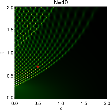
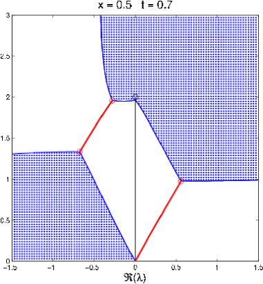
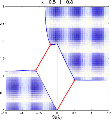
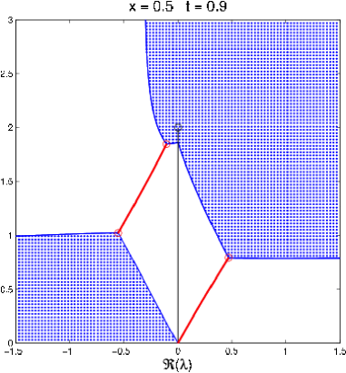
Figure 12. Evolution of the contour configuration for $G=2$. Here $x=0.5$ and $t=0.7$ through $t=0.9$ in steps of $\Delta t=0.1$. See the text for a full explanation.

Although a collision of one of the endpoints with the interval $[0,iA]$ would imply a failure of the genus-two ansatz in its original formulation (that is, without the modification described in § 3.9), it is clear by comparison with the corresponding $(x,t)$-plane plots that the secondary caustic is still far off.

Figure 13 continues the evolution. Note that between the first two frames, the band $I_{1}$ collides with the interval $[0,iA]$, so we must switch to the modified version of the genus-two ansatz described in § 3.9. Thus, a new contour arc $K_{-3}$ must be included and a new inequality $\Re(\phi(\lambda)-2i\theta^{0}(\lambda))<0$ must be satisfied along this contour. The region where this inequality is satisfied is shaded in green. Thus, the contour arc $K_{-3}$ must lie in the green shaded region, while the gaps of $K_{-1}\cup K_{-2}$ must lie in the blue shaded regions. Furthermore, the contour $C$ must from this time onward be deformed somewhat to the right to admit the passage of the band endpoint $\lambda_{1}(x,t)$ “through the branch cut”. The deformed contour $C$ we choose here, somewhat arbitrarily, is the union of the two indicated solid black line segments.

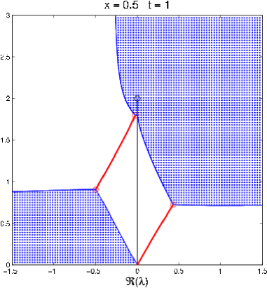
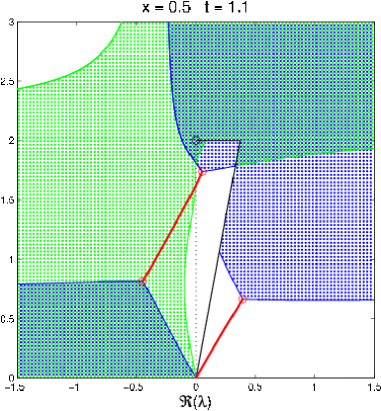
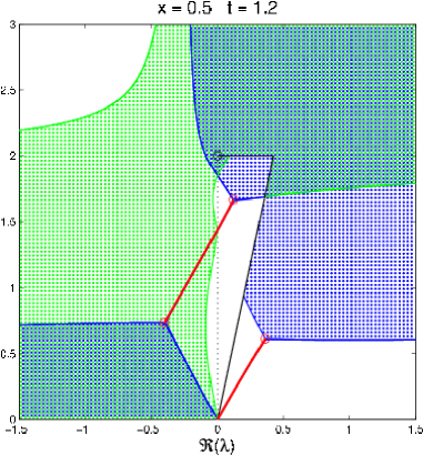
Figure 13. Same as in Figure 12 but with $t=1.0$ through $t=1.2$ in steps of $\Delta t=0.1$. See the text for a full explanation.

It is clear that in each case the bands may be complemented with gaps in the blue regions to form (along with a small interval $(-\epsilon,0)$) a closed loop. In cases where this loop necessarily cannot enclose the poles of ${\bf m}(\lambda)$ accumulating in $[0,iA]$, it is clear that a curve $K_{-3}$ lying entirely in the green shaded region may be added that passes over the top of $[0,iA]$ and forms along with parts of the above closed loop the boundary of a region containing the poles.

In Figure 14 we continue the evolution toward a curve in the $(x,t)$-plane at which the asymptotic behavior abruptly changes for the second time, where we expect to find a mathematical explanation for the secondary caustic. Note that between the last two snapshots there is a pinch-off of the green shaded region where $\Re(\phi(\lambda)-2i\theta^{0}(\lambda))<0$. When this happens, a contour lobe $K_{-3}$ that serves to bound the region containing the poles of ${\bf m}(\lambda)$ (soliton eigenvalues) and also along which the inequality $\Re(\phi(\lambda)-2i\theta^{0}(\lambda))<0$ holds can no longer exist. This is the mathematical mechanism for the development of the secondary caustic.

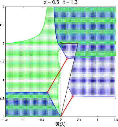
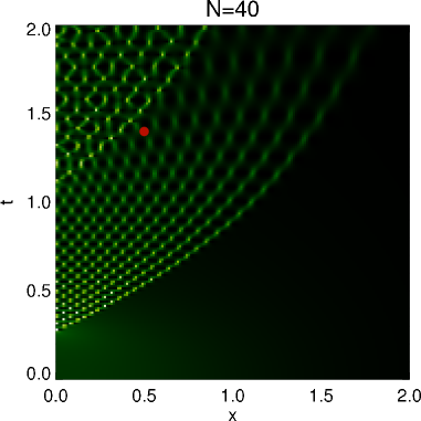
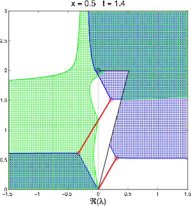
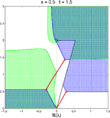
Figure 14. Same as in Figure 13, but with $t=1.3$ through $t=1.5$ in steps of $\Delta t=0.1$. See the text for a full explanation.

To demonstrate more convincingly that the secondary caustic in the numerical reconstructions of the $N$-soliton solution for large $N$ actually corresponds to the curve in the $(x,t)$-plane along which the region in which the inequality $\Re(\phi(\lambda)-2i\theta^{0}(\lambda))<0$ is pinched off at a point, we used a secant method to find, for a given $x$, the $t$-value at which $\Re(\phi(\hat{\lambda})-2i\theta^{0}(\hat{\lambda}))=0$ where $\hat{\lambda}$ is a complex root of $\phi^{\prime}(\lambda)-2i\theta^{0\prime}(\lambda)$. Level curves of $\Re(\phi(\lambda)-2i\theta^{0}(\lambda))$ passing through simple critical points like $\hat{\lambda}$ necessarily exhibit a characteristic perpendicular crossing singularity. This method yields (approximate) coordinates of points in the $(x,t)$-plane at which the configuration of level curves makes a transition between the two types of configurations illustrated in the final two frames of Figure 14. These points lie along a curve $t=t_{2}(x)$ that defines the location of the secondary caustic. Configurations corresponding to three of the points we obtained in this way are illustrated in Figure 15.

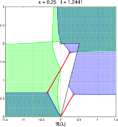
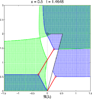
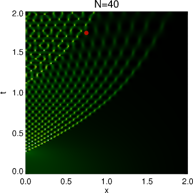
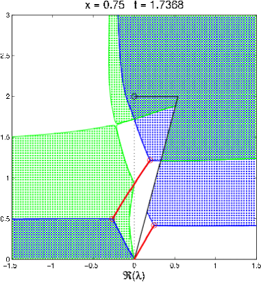
Figure 15. Configurations in which the region where the inequality $\Re(\phi(\lambda)-2i\theta^{0}(\lambda))<0$ holds is “pinched-off” delineate the secondary caustic.

6. Transition to Higher Genus

6.1. Violation of the new inequality.

According to the numerics explained in § 5, the failure of the genus-two ansatz at the secondary caustic corresponds to the equations (compare with (199)):

(214) $$\phi^{\prime}(\hat{\lambda})-2i\theta^{0\prime}(\hat{\lambda})=0\,,\hskip 14.45377pt\Re(\phi(\hat{\lambda})-2i\theta^{0}(\hat{\lambda}))=0\,.$$

We expect the critical point $\hat{\lambda}$ arising from these equations to be the origin of a new band, and to show this we need to develop the genus-four ansatz within the framework of the modified approach given in § 3.9, but where the new band appears on the contour $K_{-3}$. This gives the equations implicitly defining the endpoints as functions of $x$ and $t$ a different appearance than if the new band were assumed to lie on $K_{-1}\cup K_{-2}$. These equations turn out to define a previously unknown branch of solutions of the quasilinear system of Whitham equations (as defined in § 3.4.1).

6.2. On and beyond the secondary caustic.

6.2.1. Endpoint equations for genus four with a band on $K_{-3}$.

The modification described in § 3.9 leads to a new inequality that must be satisfied for $\lambda\in K_{-3}$. Moreover, the numerical computations in § 5 indicate that the failure of the genus-two ansatz is due to the violation of this new inequality. We then expect, similarly as in the case of the transition from genus zero to genus two across the primary caustic, that the pinching off of the inequality region $\Re(\phi(\lambda)-2i\theta^{0}(\lambda))<0$ leads to the birth of a new band and a phase transition.

In this section we describe the modifications to the endpoint equations that arise when we allow a band to lie on the arc $K_{-3}$. In particular, we suppose that there is a single band in each of the arcs $K_{0}$, $K_{-2}$, and $K_{-3}$, and we develop equations corresponding to (131) and (133)–(134) in this special case. The resulting contours of discontinuity for ${\bf P}(\lambda)$ in this situation are illustrated in Figure 16.

Figure 16. The discontinuity contours for ${\bf P}(\lambda)$ in the genus-four configuration with a band on the outer contour lobe $K_{-3}$.

To begin, consider the analytic matrix $\mathbf{M}(\lambda)$ obtained as in § 3.9 from the triple interpolation procedure. As before we introduce the function $g(\lambda)$, but now we suppose that $g(\lambda)$ is analytic except on $K_{0},K_{-1},K_{-2}$, and $K_{-3}$ along with the complex conjugates of these arcs. We then define a new unknown via $\mathbf{N}(\lambda):=\mathbf{M}(\lambda)e^{-g(\lambda)\sigma_{3}/\hbar}$. All the jump conditions relating boundary values are as before with the exception of the condition regarding boundary values on $K_{-3}$. In place of (193), we find

(215) $$\mathbf{N}_{+}(\lambda)=\mathbf{N}_{-}(\lambda)\begin{bmatrix}e^{-[g_{+}(\lambda)-g_{-}(\lambda)]/\hbar}&0\\ iP(\lambda)e^{[2iQ(\lambda)-3i\theta^{0}(\lambda)-g_{+}(\lambda)-g_{-}(\lambda)]/\hbar}&e^{[g_{+}(\lambda)-g_{-}(\lambda)]/\hbar}\end{bmatrix}.$$

Continuing to follow the steps of our earlier analysis, we arrive at a Riemann-Hilbert Problem for an unknown matrix $\mathbf{O}(\lambda)$ which has no jump discontinuities on the real intervals $(-\epsilon,0)$ and $(0,\epsilon)$, satisfies the jump conditions (91)–(92), (195), and also satisfies

(216) $$\mathbf{O}_{+}(\lambda)=\mathbf{O}_{-}(\lambda)\begin{bmatrix}e^{-[g_{+}(\lambda)-g_{-}(\lambda)]/\hbar}&0\\ iS(\lambda)e^{[2iQ(\lambda)+L(\lambda)-i\theta^{0}(\lambda)-g_{+}(\lambda)-g_{-}(\lambda)-2i\theta^{0}(\lambda)]/\hbar}&e^{[g_{+}(\lambda)-g_{-}(\lambda)]/\hbar}\end{bmatrix},\quad\text{for}\,\lambda\in K_{-3}.$$

From (216), the band and gap conditions for the arc $K_{-3}$ are slightly different from those in (96) and (97) which continue to hold in the arcs $K_{0},K_{-1}$, and $K_{-2}$. Namely, for a band in $K_{-3}$, we require

(217) $$\phi(\lambda)-2i\theta^{0}(\lambda)\equiv\,\text{imaginary constant},\quad\theta(\lambda)=\,\text{real decreasing function,}$$

while for a gap in $K_{-3}$, there must hold

(218) $$\Re(\phi(\lambda)-2i\theta^{0}(\lambda))<0,\quad\theta(\lambda)\equiv\,\text{real constant}.$$

Then, we note that $g^{\prime}(\lambda)$ must satisfy (98) in the bands not on $K_{-3}$, (99) in all gaps, (100), (101), and

(219) $$g_{+}^{\prime}(\lambda)+g_{-}^{\prime}(\lambda)=2iQ^{\prime}(\lambda)+L^{\prime}(\lambda)-3i\theta^{0\prime}(\lambda),\quad\text{for $\lambda$ in the band on $K_{-3}$}.$$

These conditions amount to a scalar Riemann-Hilbert Problem for $g^{\prime}(\lambda)$. We (re)define $C_{f}$ to be the contour $K_{0}\cup K_{-1}\cup K_{-2}\cup(-\epsilon,0)\cup C$, and we define $f(\lambda)$ as before by (102) and (103). We then make the change of variables

(220) $$h(\lambda):=g^{\prime}(\lambda)+f(\lambda).$$

We see that the function $h(\lambda)$ is characterized by (113) for bands not in $K_{-3}$, (114)–(116), and

(221) $$h_{+}(\lambda)+h_{-}(\lambda)=2iQ^{\prime}(\lambda)-3i\theta^{0\prime}(\lambda),\quad\text{in the band on $K_{-3}$}.$$

We have thus traded our scalar Riemann-Hilbert Problem to determine the unknown $g^{\prime}(\lambda)$ for one in which the unknown is $h(\lambda)$. We suppose that the endpoints of the bands

$$\lambda_{0},\lambda_{1},\ldots,\lambda_{4}$$

are known, and we define $R(\lambda)$ by

(222) $$R(\lambda)^{2}=\prod_{n=0}^{4}(\lambda-\lambda_{n})(\lambda-\lambda_{n}^{*}),$$

and the conditions (i) the branch cuts are the bands in $K_{0}$, $K_{-2}$, and $K_{-3}$ and (ii) $R(\lambda)=\lambda^{5}+O(\lambda^{4})$ as $\lambda\to\infty$. We denote the bands by $I_{0}$, $I_{1}$, and $I_{2}$. Note that $I_{2}$ has the same orientation as $K_{-3}$. Finally, we are able to solve for $h(\lambda)$ by writing it as the product of $R(\lambda)$ and a new unknown function $k(\lambda)$ as in (119). From the definition of $R(\lambda)$, the conditions on $h(\lambda)$ translate to conditions on $k(\lambda)$ as in (120)–(124) with

(223) $$k_{+}(\lambda)-k_{-}(\lambda)=\frac{2iQ^{\prime}(\lambda)-3i\theta^{0\prime}(\lambda)}{R_{+}(\lambda)},\quad\text{for $\lambda$ in the band on $K_{-3}$}.$$

Now, using the differences of boundary values of $k(\lambda)$ in (120)–(122) and (223), we can write down an explicit formula for $k(\lambda)$. We define $k_{U}(\lambda):=k_{U}^{(1)}(\lambda)+k_{U}^{(2)}(\lambda)$ where

(224) $$k_{U}^{(1)}(\lambda) :=\frac{1}{\pi}\int_{\text{bands}\subset C_{f}}\frac{Q^{\prime}(\eta)}{R_{+}(\eta)(\eta-\lambda)}\,d\eta+\frac{1}{\pi}\int_{I_{2}}\frac{Q^{\prime}(\eta)-\frac{3}{2}\theta^{0\prime}(\eta)}{R_{+}(\eta)(\eta-\lambda)}\,d\eta,$$

(225) $$k_{U}^{(2)}(\lambda) :=-\frac{1}{2i}\int_{C_{f}\setminus\text{bands}}\frac{d\eta}{R(\eta)(\eta-\lambda)}.$$

We note that we can rewrite $k_{U}^{(1)}$ as

$$k_{U}^{(1)}(\lambda)=\frac{1}{\pi}\int_{\text{bands}}\frac{Q^{\prime}(\eta)}{R_{+}(\eta)(\eta-\lambda)}\,d\eta\underbrace{-\frac{3}{2\pi}\int_{I_{2}}\frac{\theta^{0\prime}(\eta)}{R_{+}(\eta)(\eta-\lambda)}\,d\eta}_{\mathcal{I}_{U}(\lambda)}$$

Finally, $k(\lambda)$ must have the following form:

(226) $$k(\lambda):=k_{U}(\lambda)-k_{U}(\lambda^{*})^{*}.$$

A residue calculation shows that

$$k_{U}^{(1)}(\lambda)-k_{U}^{(1)}(\lambda^{*})^{*}=\frac{iQ^{\prime}(\lambda)}{R(\lambda)}+\mathcal{I}_{U}(\lambda)-\mathcal{I}_{U}(\lambda^{*})^{*},$$

hence

(227) $$k(\lambda)=\frac{iQ^{\prime}(\lambda)}{R(\lambda)}+\mathcal{I}_{U}(\lambda)-\mathcal{I}_{U}(\lambda^{*})^{*}+k_{U}^{(2)}(\lambda)-k_{U}^{(2)}(\lambda^{*})^{*}.$$

Finally, we derive the analogues of (131) by enforcing the decay condition (124). We expand the integrals appearing in (227) for large $\lambda$. We note that $\theta^{0\prime}(\lambda)\equiv i\pi$, so

$$\mathcal{I}_{U}(\lambda)=\sum_{p=0}^{5}\left[\frac{3i}{2}\int_{I_{2}}\frac{\eta^{p}}{R_{+}(\eta)}\,d\eta\right]\lambda^{-1-p}+O(\lambda^{-7})\quad\text{as}\;\lambda\to\infty.$$

Starting from the notation (129), we introduce modified moments

(228) $$\tilde{M}_{p}(\lambda_{0},\ldots,\lambda_{4}):=M_{p}(\lambda_{0},\ldots,\lambda_{4})-3\Re\left(\int_{I_{2}}\frac{\eta^{p}}{R_{+}(\eta)}\,d\eta\right)\,,$$

and we thus find that

(229) $$0=\tilde{M}_{p}(\lambda_{0},\ldots,\lambda_{4})\,,\quad\text{for $p=0,1,2$},$$

(230) $$2t=\tilde{M}_{3}(\lambda_{0},\ldots,\lambda_{4})\,,$$

(231) $$x+2t\sum_{n=0}^{4}a_{n}=\tilde{M}_{4}(\lambda_{0},\ldots,\lambda_{4})\,,$$

(232) $$x\sum_{n=0}^{4}a_{n}+2t\left(\sum_{n=0}^{4}\left(a_{n}^{2}-\frac{1}{2}b_{n}^{2}\right)+\sum_{n=0}^{4}\sum_{m=n+1}^{4}a_{m}a_{n}\right)=\tilde{M}_{5}(\lambda_{0},\ldots,\lambda_{4})\,.$$

These equations amount to real constraints that must be satisfied by the 5 complex endpoints in the upper half plane.

To ensure that $\Im(\theta(\lambda))=0$ in the gaps, we require as before that (recall that $A_{n}$ is a small counter-clockwise oriented closed contour surrounding the band $I_{n}$)

(233) $$\Re\left(\oint_{A_{n}}g^{\prime}(\eta)\,d\eta\right)=0,\quad n=1,2.$$

Additionally, we need to enforce that $\Re(\phi(\lambda))=0$ for $\lambda$ in the bands $I_{0}$ and $I_{1}$ and that $\Re(\phi(\lambda)-2i\theta^{0}(\lambda))=0$ for $\lambda\in I_{2}$. The condition

(234) $$\Re\left(\int_{\lambda_{0}}^{\lambda_{1}}[2g^{\prime}(\eta)-2iQ^{\prime}(\eta)-L^{\prime}(\eta)+i\theta^{0\prime}(\eta)]\,d\eta\right)=0\,,$$

where the contour of integration is arbitrary in the domain of analyticity of the integrand, will guarantee that $\phi(\lambda)$ is purely imaginary in the band $I_{1}$. On the other hand, we know that $\phi(\lambda)-2i\theta^{0}(\lambda)$ is guaranteed to be constant on $I_{2}$ by our construction. To ensure that this constant has zero real part, we require that the net change of the real part of $\phi(\lambda)$ across the second gap is equal to the real part of $2i\theta^{0}(\lambda_{3})$. The second vanishing condition is

(235) $$\Re\left(\int_{\lambda_{2}}^{\lambda_{3}}[2g^{\prime}(\eta)-2iQ^{\prime}(\eta)-L^{\prime}(\eta)+i\theta^{0\prime}(\eta)]\,d\eta-2i\theta^{0}(\lambda_{3})\right)=0\,,$$

where again the path of integration is arbitrary within the domain of analyticity of the integrand. Together with (229)–(232), equations (233)–(235) make up 10 real equations for the real and imaginary parts of the endpoints $\lambda_{0},\ldots,\lambda_{4}$.

The conditions (233)–(235) can be written in a simpler form that is useful for subsequent calculations. Define

(236) $$\tilde{Y}_{U}(\lambda):=Y_{U}(\lambda)+i\oint_{A_{2}}\frac{d\eta}{R(\eta)(\eta-\lambda)}\,,$$

and then set $\tilde{Y}(\lambda):=\tilde{Y}_{U}(\lambda)-\tilde{Y}_{U}(\lambda^{*})^{*}$. Therefore $\tilde{Y}(\lambda)$ is a function that is analytic where $Y(\lambda)$ is with the exception of the contours $A_{2}$ and $A_{2}^{*}$. Then, the conditions (233) are equivalent to

(237) $$\tilde{R}_{n}(\lambda_{0},\ldots,\lambda_{4}):=\Re\left(\int_{\lambda_{2n-1}}^{\lambda_{2n}}R(\eta)\tilde{Y}(\eta)\,d\eta\right)=0\,,$$

for $n=1$ and $n=2$. Similarly, the condition (234) is equivalent to

(238) $$\tilde{V}_{1}(\lambda_{0},\ldots,\lambda_{4}):=\Re\left(\int_{\lambda_{2n-2}}^{\lambda_{2n-1}}R(\eta)\tilde{Y}(\eta)\,d\eta\right)=0\,.$$

In all of these formulae, the contour of integration is arbitrary as long as it lies within the domain of analyticity of the integrand. Let $\lambda_{M}$ denote a point on $A_{2}$. Then, the condition (235) may be written as

(239) $$\tilde{V}_{2}(\lambda_{0},\ldots,\lambda_{4}):=\Re\left(\int_{\lambda_{2}}^{\lambda_{M}}R(\eta)\tilde{Y}(\eta)\,d\eta+\int_{\lambda_{M}}^{\lambda_{3}}R(\eta)\tilde{Y}(\eta)\,d\eta+2i\theta^{0}(\lambda_{2})-2\pi\int_{\lambda_{2}}^{\lambda_{M}}d\eta\right)=0\,.$$

Here the paths of integration lie in each case within the domain of analyticity of the integrand.

6.2.2. Birth of a new band upon crossing the secondary caustic.

Here we show that when $(x,t)$ is a point on the secondary caustic, so that the equations (214) hold, the equations derived above that determine the endpoints of the genus-four ansatz with band $I_{2}$ on the outer contour lobe $K_{-3}$ admit the solution where $\lambda_{0}(x,t)$, $\lambda_{1}(x,t)$, and $\lambda_{2}(x,t)$ are all equal to the corresponding endpoints for the genus-two ansatz at the same point in the $(x,t)$-plane, while $\lambda_{3}(x,t)=\lambda_{4}(x,t)=\hat{\lambda}$.

To show this we first note that the conditions defining the function $g^{\prime}(\lambda)$ in terms of the endpoints yield the same function in both the genus-two case (ignoring $\lambda_{3}$ and $\lambda_{4}$) and in the genus-four case described above (assuming $\lambda_{3}=\lambda_{4}$). Since $\lambda_{0}$, $\lambda_{1}$, and $\lambda_{2}$ are such that $g^{\prime}(\lambda)=O(\lambda^{-2})$ as $\lambda\rightarrow\infty$ (because the genus-two version of $g^{\prime}(\lambda)$ satisfies the appropriate suite of four moment conditions), we also know that the genus-four version of $g^{\prime}(\lambda)$ satisfies the corresponding suite of six moment conditions (see (229)–(232)).

It therefore remains to verify the remaining integral conditions (233)–(235) involving $g^{\prime}(\eta)$. Since the function $g^{\prime}(\eta)$ is the same whether we consider the genus-two or degenerate genus-four version, the conditions $\tilde{R}_{1}=0$ and $\tilde{V}_{1}=0$ are automatically satisfied, as these are equivalent to the conditions $R_{1}=0$ and $V_{1}=0$ satisfied by the genus-two version of $g^{\prime}(\eta)$. Furthermore, since $g^{\prime}(\eta)$ is analytic in a neighborhood of $\hat{\lambda}$, we have by Cauchy’s Theorem

(240) $$\oint_{A_{2}}g^{\prime}(\eta)\,d\eta=0\,,$$

which in particular implies that the real part is zero, so $\tilde{R}_{2}=0$ is satisfied as well. Finally, we observe that the second vanishing condition (235) is, when the point $\hat{\lambda}$ is taken as the second endpoint of the gap $\Gamma_{2}$, satisfied as a consequence of the definition (214) of the critical point characteristic of the secondary caustic. This completes the proof that each point on the secondary caustic, as defined by (214) for the genus-two ansatz, corresponds to a degeneration of an admissible genus-four configuration with $\lambda_{3}=\lambda_{4}=\hat{\lambda}$.

Showing that the points $\lambda_{3}$ and $\lambda_{4}$ separate in a direction admitting a new band $I_{2}$ between them as $t$ increases beyond the secondary caustic is slightly complicated by the fact that the Jacobian of the system of endpoint equations is singular in this case. However, a direct calculation shows that the $8\times 8$ Jacobian of all endpoint equations with the exception of (233) for $n=2$ and (235) taken with respect to the independent variables $\lambda_{0}$, $\lambda_{1}$, $\lambda_{2}$, $(\lambda_{3}+\lambda_{4})/2$, and their complex conjugates is nonsingular in the degenerate configuration when the remaining independent variables $\delta:=(\lambda_{4}-\lambda_{3})/2$ and $\delta^{*}:=(\lambda_{4}^{*}-\lambda_{3}^{*})/2$ both vanish. This reduces the problem to the study of two equations and two unknowns. It follows that near the degenerate configuration, the eliminated variables are all analytic functions of $x$, $t$, $\delta$, and $\delta^{*}$, and it can be checked that all are invariant under $\delta\rightarrow-\delta$ and $\delta^{*}\rightarrow-\delta^{*}$ independently. This actually makes them analytic functions of $x$, $t$, $\delta^{2}$, and $\delta^{*2}$.

The remaining equations are $\tilde{R}_{2}=0$ and $\tilde{V}_{2}=0$, and the left-hand sides of these are now to be considered functions of $x$, $t$, $\delta$, and $\delta^{*}$. Knowing that they admit the solution $\delta=\delta^{*}=0$ when $(x,t)$ is a point on the secondary caustic, we wish to solve them for the variables $\delta$ and $\delta^{*}$ for nearby $(x,t)$. We will show that there is a unique solution satisfying the condition that $\delta$ and $\delta^{*}$ are complex conjugates of each other for real $x$ and $t$ (there are other solutions that bifurcate from $\delta=\delta^{*}=0$ that do not have this symmetry, which is the primary source of difficulty). We define polar coordinates by

(241) $$\delta=re^{i\theta}\,,\hskip 14.45377pt\delta^{*}=re^{-i\theta}\,,$$

and consider the equations $\tilde{R}_{2}=0$ and $\tilde{V}_{2}=0$ naturally complexified (that is, the left-hand sides extended as analytic functions of four complex variables $x$, $t$, $r$, and $\theta$. Being as the complexification of $\tilde{R}_{2}$ can be written as the average of two integrals, one on a path surrounding the two endpoints $\lambda_{3}$ and $\lambda_{4}$ and the other on a path surrounding the two endpoints $\lambda_{3}^{*}$ and $\lambda_{4}^{*}$, it is easy to see that $\tilde{R}_{2}$ is an even function of $\delta$ and $\delta^{*}$ individually that vanishes when $\delta=\delta^{*}=0$, and therefore the equation $\tilde{R}_{2}=0$ has the form

(242) $$0=\alpha(x,t)r^{2}\cos(2(\theta-\beta(x,t)))+\text{quartic (and higher order) terms in $r$.}$$

This equation clearly defines two analytic curves crossing orthogonally at the origin in the real polar plane, with angles $\theta=\beta(x,t)+\pi/4+n\pi/2$.

Now, the complexified form of $\tilde{V}_{2}$ defines a multivalued function of $\delta$ and $\delta^{*}$, even when we restrict to the real subspace where these two variables are complex conjugates of each other. This comes about because the value of the integral terminating at $\lambda_{3}$ in $\tilde{V}_{2}$ can change its value if $\lambda_{3}$ and $\lambda_{4}$ are permuted. This monodromy effect can, however, be removed in the real subspace, because the deformation $(\delta,\delta^{*})\rightarrow(\delta e^{i\tau},\delta^{*}e^{-i\tau})$ for $\tau$ going from zero to $\pi$ (which exchanges the endpoints and their conjugates) simply adds to $\tilde{V}_{2}$ a copy of the function $\tilde{R}_{2}$. This suggests that in place of $\tilde{V}_{2}=0$ we can solve an equivalent modified equation that is single-valued in the real subspace. Indeed, we opt to replace $\tilde{V}_{2}=0$ by $\tilde{V}^{\#}_{2}=0$ where

(243) $$\begin{array}[]{rcl}\tilde{V}_{2}^{\#}&:=&\displaystyle\Re\left(\int_{\lambda_{M}}^{\lambda_{3}}R(\eta)\tilde{Y}(\eta)\,d\eta\right)-\frac{1}{4\pi i}\log\left(\frac{\delta}{\delta^{*}}\right)\cdot\Re\left(\oint_{A_{2}}R(\eta)\tilde{Y}_{+}(\eta)\,d\eta\right)\\ \\ &&\hskip 14.45377pt+\,\,\,\displaystyle\Re\left(\int_{\lambda_{2}}^{\lambda_{M}}R(\eta)\tilde{Y}(\eta)\,d\eta+2i\theta^{0}(\lambda_{2})-2\pi\int_{\lambda_{2}}^{\lambda_{M}}d\eta\right)\,.\end{array}$$

Here $\tilde{Y}_{+}(\eta)$ refers to the boundary value taken by $\tilde{Y}(\eta)$ on $A_{2}$ from the interior of this closed contour. Clearly the equation $\tilde{V}^{\#}_{2}=0$ has the same solutions as does $\tilde{V}_{2}=0$, subject to the condition $\tilde{R}_{2}=0$. But the function $\tilde{V}^{\#}_{2}$ has the advantage of being single-valued in the real polar plane of $(r,\theta)$. Moreover, we may write $\tilde{V}^{\#}_{2}$ in the form

(244) $$\begin{array}[]{rcl}\tilde{V}^{\#}_{2}&=&\displaystyle\Re\left(\int_{\lambda_{M}}^{\lambda_{3}}R(\eta)\tilde{Y}(\eta)\,d\eta-\frac{1}{2\pi i}\log(\delta)\oint_{A_{2}}R(\eta)\tilde{Y}_{+}(\eta)\,d\eta\right)+\frac{1}{2\pi}\log(r)\cdot\Im\left(\oint_{A_{2}}R(\eta)\tilde{Y}_{+}(\eta)\,d\eta\right)\\ \\ &&\hskip 14.45377pt+\,\,\,\displaystyle\Re\left(\int_{\lambda_{2}}^{\lambda_{M}}R(\eta)\tilde{Y}(\eta)\,d\eta+2i\theta^{0}(\lambda_{2})-2\pi\int_{\lambda_{2}}^{\lambda_{M}}d\eta\right)\,.\end{array}$$

Here we see that the first term of $\tilde{V}^{\#}_{2}$ is complexified as an analytic function of $\delta^{2}$ and $\delta^{*2}$ individually. Therefore it has an expression in the real polar plane of the form $f(x,t)+O(r^{2})$. The complexification of the second term, while single-valued when $\delta$ and $\delta^{*}$ are complex conjugates of one another, is not single-valued in a full $\mathbb{C}^{2}$ neighborhood of $\delta=\delta^{*}=0$. Therefore it cannot have a two-variable Taylor expansion; however the factor multiplying $\log(r)$ clearly is an even analytic function of both $\delta$ and $\delta^{*}$ that vanishes when $\delta=\delta^{*}=0$ (this is of course just the complexification of the harmonic conjugate $\tilde{R}_{2}$). Consequently, in the real polar plane we have

(245) $$\tilde{V}^{\#}_{2}=\frac{\alpha(x,t)}{2\pi}r^{2}\log(r)\sin(2(\theta-\beta(x,t)))+\gamma(x,t)+O(r^{2})\,,$$

where $\gamma(x,t)$ is an analytic function of $x$ and $t$ that vanishes to first order on the secondary caustic; it is the value of $\tilde{V}^{\#}_{2}$ given by (244) evaluated with all endpoints in the degenerate configuration. Equating this to zero, we see that the balance must occur between the $r^{2}\log(r)$ term and the constant term, so the the distance from the secondary caustic scales as $r^{2}\log(r)$ as the new band is born. The curve described by (245) near the origin in the polar plane consists of two approximately hyperbolic branches with asymptotes rotated from the curves described by the equation $\tilde{R}_{2}=0$ by $\pi/4$. Thus, we obtain for each point $(x,t)$ sufficiently close to the secondary caustic a pair of opposite solutions for $\delta=re^{i\theta}$. As $\gamma(x,t)$ changes sign, the two points come together at $\delta=0$ and then go back out along the perpendicular direction.

Determination of the sign of $\gamma(x,t)$ analogous to what is carried out in [10] is then needed to show that the points $\lambda_{3}(x,t)$ and $\lambda_{4}(x,t)$ separate in the direction conducive to the completion of a genus-four ansatz as long as $x$ decreases (or $t$ increases) as the secondary caustic is crossed. Combining these steps completes the proof that upon crossing the secondary caustic the asymptotic description of the $N$-soliton is given in terms of Riemann theta functions of genus four.

We also note that the equations $\tilde{R}_{2}=0$ and $\tilde{V}_{2}=0$ imply that the new band $I_{2}$ and the boundary curves of the region where the inequality $\Re(\phi(\lambda)-2i\theta^{0}(\lambda))<0$ holds are trajectories of the quadratic differential $R(\eta)^{2}\tilde{Y}_{+}(\eta)^{2}\,d\eta^{2}$, while the other two bands and the boundaries of the region where the inequality $\Re(\phi(\lambda))<0$ holds are trajectories of $R(\eta)^{2}Y_{-}(\eta)^{2}\,d\eta^{2}$.

6.2.3. Whitham equations.

Recall from § 3.4.1 that for arbitrary even genus $G$ (including $G=4$ as a special case), if the endpoints occur along $K_{0}\cup K_{-1}$ or $K_{0}\cup K_{-1}\cup K_{-2}$, then the endpoints implicitly defined as functions of $(x,t)$ via the relations $E_{1}=\cdots=E_{2G+2}=0$ satisfy a universal set of quasilinear partial differential equations, namely the Whitham equations (159) with complex characteristic velocities given as functions of the endpoints only via (160).

We have just seen, however, that with

(246) $$\begin{array}[]{rcl}\tilde{E}_{1}&:=&\tilde{V}_{1}\,,\\ \\ \tilde{E}_{2}&:=&\tilde{R}_{1}\,,\\ \\ \tilde{E}_{3}&:=&\tilde{V}_{2}\,,\\ \\ \tilde{E}_{4}&:=&\tilde{R}_{2}\,,\\ \\ \tilde{E}_{n}&:=&\tilde{M}_{n-5}\,,\hskip 14.45377pt\text{for $n=5,6,7$}\,,\\ \\ \tilde{E}_{8}&:=&\tilde{M}_{3}-2t\,,\\ \\ \tilde{E}_{9}&:=&\displaystyle\tilde{M}_{4}-x-2t\sum_{n=0}^{4}a_{n}\,,\\ \\ \tilde{E}_{10}&:=&\displaystyle\tilde{M}_{5}-x\sum_{n=0}^{4}a_{n}-2t\left(\sum_{n=0}^{4}\left(a_{n}^{2}-\frac{1}{2}b_{n}^{2}\right)+\sum_{n=0}^{4}\sum_{m=n+1}^{4}a_{m}a_{n}\right)\,,\end{array}$$

the conditions $\tilde{E}_{1}=\cdots=\tilde{E}_{10}=0$ determining the endpoints $\lambda_{0},\ldots,\lambda_{4}$ in the genus-four configuration just beyond the secondary caustic have a different form than the relations $E_{1}=\cdots=E_{10}=0$ (for $G=4$) from § 3.4.1. In particular, a configuration $\lambda_{0}(x,t),\ldots,\lambda_{5}(x,t)$ satisfying $E_{1}=\cdots=E_{10}=0$ does not satisfy the equations $\tilde{E}_{1}=\cdots=\tilde{E}_{10}=0$. Nonetheless, these latter conditions also determine implicitly functions $\lambda_{0}(x,t),\ldots,\lambda_{5}(x,t)$ satisfying exactly the same Whitham equations.

Theorem 1.

Any continuously differentiable solution $\lambda_{0}(x,t),\ldots,\lambda_{4}(x,t)$ of $\tilde{E}_{1}=\cdots=\tilde{E}_{10}=0$ satisfies the Whitham equations (159) with complex characteristic velocities given by (160) in any region of the $(x,t)$-plane where the endpoints are distinct.

Proof.

We complexify the functions $\tilde{E}_{n}$, letting $\vec{v}$ denote the vector $(\lambda_{0},\ldots,\lambda_{4},\lambda_{0}^{*},\ldots,\lambda_{4}^{*})^{T}$ of endpoints and their complex conjugates, viewed as independent variables. Then, direct calculations show that, by analogy with (153),

(247) $$\frac{\partial}{\partial v_{k}}(R(\eta)\tilde{Y}(\eta))=-\frac{1}{2}\tilde{Y}(v_{k})\frac{R(\eta)}{\eta-v_{k}}\,,$$

and by analogy with (154) we have

(248) $$\tilde{Y}(v_{k})=4i\frac{\partial\tilde{M}_{0}}{\partial v_{k}}\,,$$

so that

(249) $$\frac{\partial\tilde{E}_{n}}{\partial v_{k}}=-i\frac{\partial\tilde{M}_{0}}{\partial v_{k}}\left[\int_{\lambda_{n-1}}^{\lambda_{n}}\frac{R(\eta)\,d\eta}{\eta-v_{k}}-\int_{\lambda_{n}^{*}}^{\lambda_{n-1}^{*}}\frac{R(\eta)\,d\eta}{\eta-v_{k}}\right]=J_{nk}(\vec{v})\frac{\partial\tilde{M}_{0}}{\partial v_{k}}\,,$$

for $n=1$, $n=2$, and $n=4$, where $J_{nk}(\vec{v})$ are exactly the same matrix elements as defined for $G=4$ by (155). The corresponding calculation for partial derivatives of $\tilde{E}_{3}=\tilde{V}_{2}$ is slightly more complicated due to the appearance of terms explicitly depending on $\lambda_{2}$ and $\lambda_{2}^{*}$; however since

(250) $$\frac{\partial}{\partial\lambda_{2}}\left[2i\theta^{0}(\lambda_{2})-2\pi\int_{\lambda_{2}}^{\lambda_{M}}d\eta\right]=0\,,$$

in fact (249) holds for $n=3$ as well. Next, by another direct calculation, we find that by analogy with (156),

(251) $$\frac{\partial\tilde{E}_{n}}{\partial v_{k}}=\frac{1}{2}\tilde{E}_{n-1}+v_{k}\frac{\partial\tilde{E}_{n-1}}{\partial v_{k}}\,,\hskip 14.45377pt\text{for $6\leq n\leq 10$}$$

so that on a solution we have

(252) $$\frac{\partial\tilde{E}_{n}}{\partial v_{k}}=v_{k}^{n-1}\frac{\partial\tilde{E}_{5}}{\partial v_{k}}=v_{k}^{n-1}\frac{\partial\tilde{M}_{0}}{\partial v_{k}}=J_{nk}(\vec{v})\frac{\partial\tilde{M}_{0}}{\partial v}\,,\hskip 14.45377pt\text{for $5\leq n\leq 10$\,,}$$

where again the matrix elements $J_{nk}(\vec{v})$ are precisely the same as defined by (157). Therefore, the elements $\partial\tilde{E}_{n}/\partial v_{k}$ are assembled into the Jacobian matrix having the factorized form:

(253) $$\frac{\partial\vec{\tilde{E}}}{\partial\vec{v}}={\bf J}(\vec{v})\cdot\text{diag}\left(\frac{\partial\tilde{M}_{0}}{\partial v_{1}},\dots,\frac{\partial\tilde{M}_{0}}{\partial v_{10}}\right)\,,$$

where the factor ${\bf J}(\vec{v})$ is exactly the same function of $\vec{v}$ as in the case studied in § 3.4.1. Noting that the partial derivatives $\partial\tilde{E}_{n}/\partial x$ and $\partial\tilde{E}_{n}/\partial t$ are all identical expressions in terms of $\vec{v}$ as in § 3.4.1, it then follows by application of Cramer’s rule that

(254) $$\frac{\partial v_{k}}{\partial t}+c_{k}(\vec{v})\frac{\partial v_{k}}{\partial x}=0\,,\hskip 14.45377pt\text{for $k=1,\ldots,10$\,,}$$

where the characteristic speeds are exactly the same functions of $\vec{v}$ (see (160)) as in § 3.4.1.

To reiterate, the only difference between the derivation here and that in the case when no endpoints lie on $K_{-3}$ is in the diagonal factor of the Jacobian consisting of the partial derivatives $\partial\tilde{M}_{0}/\partial v_{k}$, which certainly are different functions of $\vec{v}$ than the derivatives $\partial M_{0}/\partial v_{k}$. However, this diagonal factor cancels out of the Cramer’s rule formula for the characteristic velocities $c_{k}(\vec{v})$. Note that the condition that the diagonal factor is nonsingular is, due to (248), equivalent to the function $R(\eta)\tilde{Y}(\eta)$ which defines the bands vanishing exactly like a square root at the band endpoints. ∎

7. Conclusion

In this paper we have done the following things.

• We used a numerical linear algebra method for computing the $N$-soliton for several values of $N$ as large as $N=40$, plotted the results and described the phenomena of macrostructure, microstructure, and phase transitions (caustic curves) that become more well-defined as $N\rightarrow\infty$.

• We have described a new modification of the asymptotic technique first used in [10] to analyze the $N$-soliton for large $N$ that gives an improved error estimate of $O(N^{-1})$ over the cruder estimate of $O(N^{-1/3})$ reported in [10].

• We analyzed the Fourier power spectrum of the $N$-soliton in the genus-zero region before the primary caustic and related the results to supercontinuum generation of coherent broadband spectra from narrow-band sources in optical fibers with weak anomalous dispersion.

• We computed numerically for the first time the bands of discontinuity of $g^{\prime}(\lambda)$ in the genus-two region beyond the primary caustic and pointed out the phenomenon of a band crossing the locus of accumulation of discrete eigenvalues for the $N$-soliton.

• We introduced a new multi-interpolant asymptotic procedure that allows the genus-two ansatz for $g(\lambda)$ to be continued through the discrete eigenvalues, proving that this phenomenon is not the cause of the secondary caustic.

• We observed numerically the failure of a new inequality associated with the multi-interpolant approach that becomes necessary once a band crosses the discrete spectrum, and we gave evidence that this failure is the mathematical mechanism for the secondary caustic phase transition.

• We have shown that, under the assumption that the new inequality indeed fails as we have observed numerically, the secondary caustic represents a change of genus from $G=2$ to $G=4$ but with new topological features of the genus-four ansatz for $g(\lambda)$ that have not been seen before. We also proved that despite the unusual appearance of the implicit relations defining the band endpoints in this case, the endpoints still satisfy the Whitham equations.

The nature of the mathematical mechanism for the secondary caustic leads us to hypothesize that there could easily be an infinite number of caustic curves in the $(x,t)$-plane of the $N$-soliton in the large $N$ limit. The scenario we imagine is the following: as $t$ increases for fixed $x>0$, the new band $I_{2}$ that we have shown opens up upon crossing the secondary caustic drifts toward the imaginary interval $[0,iA]$ of accumulation of discrete eigenvalues. When $I_{2}$ meets this interval, the analysis fails once again until it is rescued (in analogy with the modification we introduced in § 3.9) by adjoining a new contour lobe, $K_{-5}$, enclosing a region $D_{-5}$ adjacent to $D_{-3}$ in which the correct interpolation formula to use is the analogue of (192) with the term $-3i\theta^{0}(\lambda)$ in the exponent replaced by $-5i\theta^{0}(\lambda)$. Along $K_{-5}$ we require a new inequality, namely $\Re(\phi(\lambda)-4i\theta^{0}(\lambda))<0$. The region in which this inequality holds eventually pinches off (a tertiary caustic), and the situation is resolved by introducing a new band $I_{3}$ on $K_{-5}$ which results in local dynamics described by Riemann theta functions of genus six. The reader can then imagine that the process repeats again and again. The $k$th caustic curve is described by eliminating $\hat{\lambda}$ from the equations

(255) $$\phi^{\prime}(\hat{\lambda})-2i(k-1)\theta^{0\prime}(\hat{\lambda})=0\,,\hskip 14.45377pt\Re(\phi(\hat{\lambda})-2i(k-1)\theta^{0}(\hat{\lambda}))=0\,.$$

The formula for $\phi(\lambda)$ of course changes each time a caustic is crossed and a new band is added. Thus, a harbinger of a developing caustic curve is a recently born band meeting the imaginary axis. This can be detected just by observing the wave field as long as (like we see in the numerical constructions of $g(\lambda)$ in the genus-two case) the endpoint crossing the imaginary axis has an imaginary part much larger than those of all other endpoints. In this case, the wave field, although locally described by Riemann theta functions of some even genus $G>0$, is well-approximated by a complex exponential function $e^{i(kx-\omega t)/\hbar}$ (because the genus is “almost” zero), and the real part of the dominant endpoint is proportional to the wavenumber $k$. Thus a sign change of $k$, which could be detected by local spectral analysis, indicates the dominant endpoint crossing the imaginary axis, an event that precedes the formation of a new caustic.

We want to stress that the mechanism for all of the caustics beyond the primary caustic depends in a crucial way on the discrete nature of the spectrum for the $N$-soliton, which causes us to reinvent our method of analysis each time a band wants to cross the discrete spectrum. Significantly, if we chose to begin our analysis by assuming that there is no essential cost in the limit $\hbar\rightarrow 0$ for analyzing the formal continuum-limit problem for $\tilde{\bf P}(\lambda)$ (in which we simply neglect the difference between the discrete spectral measure and its weak limit as $N\rightarrow\infty$) in place of the exact Riemann-Hilbert problem for ${\bf P}(\lambda)$, we would not need to modify our analysis if a band crosses the spectrum, and we would not need to introduce the new inequality $\Re(\phi(\lambda)-2i\theta^{0}(\lambda))<0$ that leads to the secondary caustic. In other words, the formal continuum-limit problem corresponds to a solution $\tilde{\psi}_{N}(x,t)$ of the focusing nonlinear Schrödinger equation (3) that accurately resembles the $N$-soliton $\psi_{N}(x,t)$ for $(x,t)$ in the region before the secondary caustic, but not beyond. In particular, the solution obtained from the formal continuum-limit problem does not experience any phase transition at all when the $N$-soliton experiences the secondary caustic. Of course, as the formal continuum-limit problem may break the even symmmetry of the $N$-soliton (recall § 3.2.2) we have no solid grounds for expecting any similarity between $\psi_{N}(x,t)$ and $\tilde{\psi}_{N}(x,t)$ for any $x$ and $t$, and therefore it seems to us that we must therefore regard the correspondence before the secondary caustic as a lucky coincidence.

8. Acknowledgements

Both authors would like to thank Jinho Baik, Tony Bloch, Jeff DiFranco, and Guada Lozano for contributing to this work through discussions in meetings of a weekly Working Group in Integrable Systems and Asymptotics held at the University of Michigan; these meetings provided a great forum for our thought process. The second author gratefully acknowledges the support of the National Science Foundation under grants DMS-0103909 and DMS-0354373.

References

-
[1]
J. Baik, T. Kriecherbauer, K. T.-R. McLaughlin, and P.
D. Miller, Discrete Orthogonal Polynomials: Asymptotics and
Applications, accepted for publication in the Annals of
Mathematics Studies, Princeton University Press, 2005. Draft from
2003 posted on
arXiv:math.CA/0310278. - [2] J. C. Bronski and J. N. Kutz, “Numerical simulation of the semi-classical limit of the focusing nonlinear Schrödinger equation”, Phys. Lett. A, 254, 325–336, 2002.
- [3] H. D. Ceniceros, “A semi-implicit moving mesh method for the focusing nonlinear Schrödinger equation”, Comm. Pure Appl. Anal. 1, 1–18, 2002.
- [4] H. D. Ceniceros and F.-R. Tian, “A numerical study of the semi-classical limit of the focusing nonlinear Schrödinger equation”, Phys. Lett. A, 306, 25–34, 2002.
- [5] S. R. Clarke and P. D. Miller, “On the semi-classical limit for the focusing nonlinear Schrödinger equation: sensitivity to analytic properties of the data,” Proc. R. Soc. Lond. A, 458, 135–156, 2002.
- [6] I. Cristiani, R. Tediosi, L. Tartara, and V. Degiorgio, “Dispersive wave generation by solitons in microstructured optical fibers”, Optics Express, 12, 124–135, 2004.
- [7] P. Deift and X. Zhou, “A steepest-descent method for oscillatory Riemann-Hilbert problems: asymptotics for the mKdV equation”, Ann. Math., 137, 295–368, 1993.
- [8] J. M. Dudley and S. Coen, “Coherence properties of supercontinuum spectra generated in photonic crystal and tapered optical fibers”, Optics Lett., 27, 1180–1182, 2002.
- [9] A. Ferrando, E. Silvestre, J. J. Miret, and P. Andrés, “Nearly zero ultraflattened dispersion in photonic crystal fibers”, Optics Lett., 25, 790–792, 2000.
- [10] S. Kamvissis, K. T.-R. McLaughlin, and P. D. Miller, Semiclassical Soliton Ensembles for the Focusing Nonlinear Schrödinger Equation, Annals of Mathematics Studies, volume 154, Princeton University Press, Princeton, 2003.
- [11] P. D. Miller, “Asymptotics of semiclassical soliton ensembles: rigorous justification of the WKB approximation”, Internat. Math. Res. Notices, 383–454, 2002.
- [12] P. D. Miller and S. Kamvissis, “On the semiclassical limit of the semiclassical focusing nonlinear Schrödinger equation”, Phys. Lett. A, 247, 75–86, 1998.
- [13] J. Satsuma and N. Yajima, “Initial value problems of one-dimensional self-modulation of nonlinear waves in dispersive media”, Supp. Prog. Theo. Phys., 55, 284–306, 1974.
- [14] A. Tovbis and S. Venakides, “The eigenvalue problem for the focusing nonlinear Schrödinger equation: new solvable cases”, Phys. D, 146, 150–164, 2000.
- [15] A. Tovbis, S. Venakides, and X. Zhou, “On semiclassical (zero dispersion limit) solutions of the focusing nonlinear Schrödinger equation”, Comm. Pure Appl. Math., 57, 877–985, 2004.
- [16] V. E. Zakharov and A. B. Shabat, “Exact theory of two-dimensional self-focusing and one-dimensional self-modulation of waves in nonlinear media”, Sov. Phys. JETP, 34, 62–69, 1972.