Chaotic and Regular Motion in Dissipative Gravitational Billiards

Abstract

We consider the motion of a particle subjected to the constant gravitational field and scattered inelasticaly by hard boundaries which possess the shape of parabola, wedge, and hyperbola. The billiard itself performs oscillations. The linear dependence of the restitution coefficient on the particle velocity is assumed. We demonstrate that this dynamical system can be either regular or chaotic, which depends on the billiard shape and the oscillation frequency. The trajectory calculations are compared with the experimental data; a good agreement has been achieved. Moreover, the properties of the system has been studied by means of the Lyapunov exponents and the Kaplan-Yorke dimension. Chaotic and nonuniform patterns visible in the experimental data are interpreted as a result of large embedding dimension.

From the mathematical point of view, billiards constitute an interesting class of dynamical systems because they exhibit – despite their simplicity – a variety of nonlinear phenomena, including both regular tori and completely chaotic, dense trajectories. Some of them are quite realistic and have a direct physical importance. An example of such a system is the gravitational billiard in which a point-mass particle bounces within a container of a given shape and its motion between the bounces is not free but ballistic. Obviously, the dynamics depends on the billiard shape. For the parabolic boundary the system is integrable and all orbits are regular and stable. Historically, the first study on the gravitational billiards has been performed for the two-dimensional wedge, defined as two intersecting straight lines leh ; mil . The motion in the wedge is fully chaotic if its vertex angle is larger than $\pi/2$ woj , otherwise there is a coexistence of regular and chaotic behaviour. Those findings were successfully tested experimentally miln . The chaotic, as well as regular, dynamics is present also for the hyperbolic shape of the gravitational billiard which involves both the wedge and the parabola as its asymptotic limits fer . The chaotic component prevails for shapes close to the wedge.

All the above approaches assumed that the collisions between the particle and the billiard boundary were elastic. It is natural to require that, in order to make the problem more realistic, one should take into account the energy loss and allow for the energy exchange between the particle and the wall. Such handling of the dissipation is known in nuclear physics as the wall formula blo , derived in the framework of the liquid drop model. The atomic nucleus can then be modeled as a billiard possessing the oscillating boundary given by the Legendre polynomials of various kinds blo1 which lead to both regular and chaotic motion blo2 . Similar investigations for the gravitational billiards were lacking. Only recently they have been studied – experimentally – under the assumption that the energy loss during the collisions is to be compensated, on the average, by the motion of the container fel . The authors of Ref.fel constructed three aluminum containers with parabolic, wedge, and hyperbolic shape which exercised the horizontal oscillations. Inside a ball of steel was scattered from the boundaries and a camera registered the position of each bounce and the ball velocity. The results clearly indicate the regular motion for the parabola and the chaotic one for the wedge; they also suggest some sort of regularity for the hyperbola at a small driving frequency.

In this Letter we present a theoretical study of the inelastic gravitational billiards with a time-dependent driving. To the best of our knowledge, it is the first theoretical approach to these – very realistic – systems. The billiard shapes and parameters of the dynamical system have been so chosen to enable us a direct comparison with the experimental data fel . Then we assume the following boundaries: $f(x)=a(x-\bar{x})^{2}+c$ (the parabola), $f(x)=b|x-\bar{x}|+c$ (the wedge), and $f(x)=\sqrt{\alpha(1+\beta(x-\bar{x})^{2})}-\delta$ (the hyperbola), where $a=0.26$ cm^-1, $b=1.85$, $c=0.63$ cm, $\alpha=40.3$ cm², $\beta=0.08$ cm^-2, and $\delta=4.45$ cm. The containers oscillate horizontally: $\bar{x}(t)=-A\sin\omega t$, where $A$ is the amplitude and $\omega=2\pi f$ is the oscillation frequency. Inside the container the particle is subjected to the constant gravitational acceleration $g$. Collisions with the boundaries result in the energy loss, quantified by the restitution coefficient $r\in[0,1]$ which is defined as a ratio of the absolute values of the velocity after and before the collision. The case $r=1$ corresponds to the elastic collision. It is difficult to decide a priori which value for $r$ should be assumed. An experiment with steel particles bounced on a steel block gives $r=0.93$ kud . However, taking into account effects connected with the sharing of energy between rotation and translation during the collision reduces this coefficient substantially and the effective $r$ appears of about 0.7. Moreover, $r$ can depend on the velocity and on the scattering angle kud . The authors of Ref.fel suggest $r=0.9$. In the following, we will try to draw some conclusions about the restitution coefficient from the comparison of our results with the experimental data of Ref.fel .

Let us assume that the particle hits the boundary at the time $t_{0}$ with the velocity ${\bf v}^{C}_{0}$, determined in respect to the frame connected with the billiard, and the collision point is $(x^{C}_{0},y^{C}_{0}=f(x^{C}_{0}))$. The transformation of particle velocities at this point, ${\bf v}^{C}_{0}\to{\bf v}^{C}_{1}$, has the following form

$${\bf v}^{C}_{1}=r({\bf v}^{C}_{0}-2{\bf u}({\bf v}^{C}_{0}\cdot{\bf u})),$$ (1)

where the components of the versor normal to the boundary, ${\bf u}$, depend on $x^{C}_{0}$ and are given by: $u_{x}=-f^{\prime}(x^{C}_{0})/h(x^{C}_{0})$ and $u_{y}=1/h(x^{C}_{0})$ with $h(x^{C}_{0})=\sqrt{1+f^{\prime 2}(x^{C}_{0})}$. The particle, after being reflected from the boundary, moves along the ballistic trajectory:

$$\begin{split}&x^{C}(t)=x^{C}_{0}+v^{C}_{x,1}(t-t_{0})+A\sin\omega t-A\sin\omega t_{0}\\ &y^{C}(t)=y^{C}_{0}+v^{C}_{y,1}(t-t_{0})-g(t-t_{0})^{2}/2,\end{split}$$ (2)

for $t>t_{0}$, up to the next section of this curve with the boundary: $(x^{C}(t_{1}),y^{C}(t_{1}))=(x^{C}_{1},y^{C}_{1})$. The subsequent applying of Eqs.(1) and (2) produces a set of collision events which take place at times $t_{n}$. The time evolution can be characterized by the vector ${\bf X}_{n}=(x^{C}_{n},y^{C}_{n},v^{C}_{x,n},v^{C}_{y,n})$ in the four-dimensional phase space, where the velocities are taken just before the consecutive bounces. Therefore, we can restrict the dynamics to the billiard boundary and describe it in terms of the following time-dependent mapping:

$${\bf X}_{n+1}={\cal P}_{n}({\bf X}_{n}).$$ (3)

The above expressions have been formulated in the billiard coordinates because then the simple velocity transformation rule (1) holds. The transformation to the laboratory frame is straightforward: $x=x^{C}-A\sin\omega t$ and $v_{x}=v^{C}_{x}-A\omega\cos\omega t$; $y$-components remain the same. The equation for the boundary $f(x)$ reduces the 4-dimensional phase space, in which ${\cal P}_{n}$ is defined, to the 3-dimensional manifold.

For various shapes of the billiard and various driving forces, the mapping ${\cal P}_{n}$ can represent either a regular cycle or a strange attractor. The static, elastic billiard with the parabolic shape is always regular and possesses two stable orbits: the horizontal orbit, connected with the symmetric bouncing between the left and the right part of the boundary at the same height, and the vertical one which involves the top of the parabola kor . In our case the limit cycle corresponds to the fixed point of the mapping ${\cal P}_{n}^{2}$ and can be obtained analytically by solving the equation ${\bf X}^{*}={\cal P}^{2}({\bf X}^{*})$. The detailed equations are complicated and will not be presented here. As a result, we yield the stable horizontal orbit which moves to and fro together with the container. The vertical orbit of the elastic billiard shrinks now to a single point. The time interval between consecutive bounces of the horizontal orbit (2-point attractor on the boundary) $\tau^{*}=\pi/\omega$, moreover $v_{y}=\pi g/2\omega$; these quantities depend neither on the restitution coefficient $r$ nor on the billiard shape. For the parabolic shape the agreement of $\tau^{*}$ with the data fel is very good. For $r=0.9$ we get the height of the orbit $y=158$ cm which exceeds by far the experimental value $y\approx 7.5$ cm. The latter value can be obtained if we assume $r=0.43$. Therefore, the restitution coefficient seems to be well established by the experiment at the value $r=0.43$ and we can try to apply it in numerical calculations for the other shapes. However, all trajectories calculated in this way, both for the wedge and for the hyperbola, do collapse to the bottom of the billiard instantly. Apparently, the assumption that the restitution coefficient can be approximated by a constant cannot be maintained in the present problem.

In the following we assume that the damping factor depends linearly on the particle velocity and then the restitution coefficient is of the form:

$$r=1-|{\bf v}^{C}|/v_{cr}$$ (4)

if $r>0.01$; otherwise (for very large velocities) $r=0.01$. The parameter $v_{cr}$ can be determined by comparison with the data. The parabola case is especially useful for that purpose because it must be characterized by a simple cycle. The data fel seem to confirm the presence of a cycle though it appears in a strongly diffused form which may result both from the low resolution in the experiment (e.g. due to the surface roughness) and from the rotational degree of freedom, not taken into account in the calculations. We get the position of the 2-point attractor in agreement with the data for $v_{cr}=390$ cm/s. We apply this value in the calculations for the other shapes.

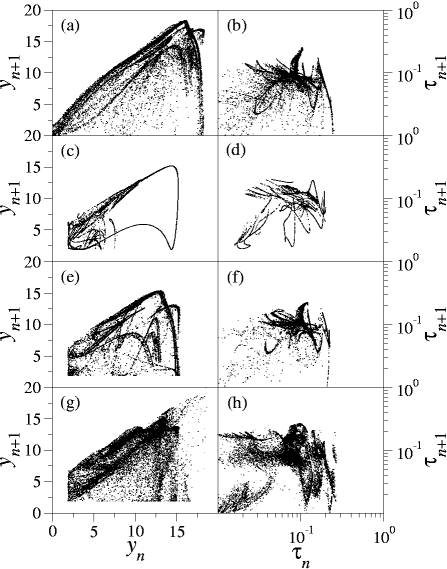
Figure 1: The coordinate $y$ of a collision point vs. $y$ for the previous collision (left column) and the time of flight between two subsequent collisions (right column). The following cases are presented: the wedge with $f=6.6$ Hz ((a) and (b)) and the hyperbola with: $f=4.5$ Hz ((c) and (d)), $f=5.8$ Hz ((e) and (f)), and $f=8$ Hz ((g) and (h)). The units are: [cm] for $y$ and [s] for the time.

Fig.1 presents some properties of the map ${\cal P}_{n}$ – the height $y$ and the time interval between consecutive bounces $\tau_{n}=t_{n}-t_{n-1}$ – for the wedge and the hyperbola which is driven by three different frequencies. Each figure represents a single trajectory, evolved up to $t=2\cdot 10^{3}$ s which corresponds to about $2\cdot 10^{4}$ collisions with the boundary. The plot of $y$ for the wedge is strongly nonuniform and indicates a high degree of chaoticity. The most of the points is concentrated just above the line $y_{n+1}=y_{n}$ and the fractal structure is hardly visible. The figure can be directly compared with the data (see Fig.3 in Ref.fel ); the similarity is striking though the calculated quantities are extended to slightly larger values than the data. The nonuniformity is clearly visible also in the plot of the time intervals and the region close to the point $(0.09,0.09)$ is distinguished. The experimental data exhibit the same pattern. The hyperbola involves the wedge as well as the parabola as its limiting shapes and one can expect both shapes influence the results of the dynamical calculations for the hyperbola. For the low driving frequency $f=4.5$ Hz (Fig.1c, d) the particle abides close to the bottom of the billiard which can be well approximated by the parabola. That results in apparently regular pattern. However, a stochastic ingredient, similar as in Fig.1a which corresponds to the wedge, is also visible in Fig.1c. In the experimental data the chaotic component connected with the wedge seems to be absent completely. Instead, long-time tails in the plot of time intervals, possessing the intermittent structure, are observed, as well as very small values of the height $y$. Then the experimental results suggest a more regular motion than the calculations predict. For the larger frequency $f=5.8$ Hz (Fig.1e, f) the chaotic behaviour is overwhelming. The bands typical for the strange attractors are visible; it is not the case for the experimental data but such subtle structures may be smeared due to the low resolution. The bands vanish completely if we make the frequency still larger. Fig.1 g, h shows that it happens for $f=8$ Hz (the case not studied experimentally) and the picture is similar to that for the wedge. However, it is not generally true that the degree of chaoticity rises with the frequency: for $f>8$ Hz the motion becomes regular again.

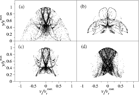
Figure 2: The normalized coordinate $y$ of a collision point vs. the normalized tangential velocity $v_{t}$ at the same point for the following cases: the wedge with $f=6.6$ Hz (a) and the hyperbola with $f=4.5$ Hz (b), with $f=5.8$ Hz (c), and with $f=8$ Hz (d).

Some additional information about the phase space structure can be obtained by plotting the position $y$ versus the tangential velocity after the collision, $v_{t}$, at collision points, normalized by $y^{max}$ and $v_{t}^{max}$, respectively. The quantities $y^{max}$ and $v_{t}^{max}$ mean the largest possible values of $y$ and $v_{t}$ at each collision, obtained under the assumption that the particle is either at rest or bounces almost horizontally at the bottom of the billiard. Therefore, the region around $v_{t}=0$ corresponds to the head-on collisions which may result in instability of the motion and the onset of the chaotic behaviour. For the parabolic shape we have obtained 2-point limiting cycle, corresponding to very small values of the tangential velocity: $(v_{t}/v_{t}^{max},y/y^{max})=(\pm 0.044,0.39)$. The experimental result presents itself as a narrow band, due to the noise in the system. Results of the calculations for the other shapes are presented in Fig.2. The case of the hyperbola for the largest frequency $f=8$ Hz shows the greatest disorder (Fig.2d) whereas the trajectory for the wedge (Fig.2a) is able to fill the entire region which is allowed by the energy partition rule fel . The figure for the hyperbola at the intermediate frequency $f=5.8$ Hz (Fig.2c) indicates, in turn, a pronounced fractal structure. On the other hand, the pattern for $f=4.5$ Hz is predominantly regular (Fig.2b). However, a vertical strip at small $|v_{t}|$ bears apparent signs of chaos. Indeed, a magnification of this region reveals the fractal structure. Also the experiment fel distinguishes the region of small tangential velocities for this case but the lack of any fine structure in the data prevents detailed comparisons.

Table 1: The Liapunov exponents for the mapping ${\cal P}_{n}$ and the Kaplan-Yorke dimension for the parabola (p), the wedge (w), and the hyperbola with frequencies: f=4.5 Hz (h1), f=5.8 Hz (h2), and f=8 Hz (h3).

	$\lambda_{1}$	$\lambda_{2}$	$\lambda_{3}$	$\lambda_{4}$	$D_{KY}$
p	$-0.408$	$-0.579$	$-0.579$	$-2.17$	$0.00$
w	$0.447$	$-0.288$	$-1.17$	$-1.98$	$2.14$
h1	$0.208$	$-0.579$	$-1.05$	$-1.42$	$1.36$
h2	$0.367$	$-0.394$	$-1.21$	$-1.78$	$1.93$
h3	$0.611$	$-0.0637$	$-1.05$	$-2.08$	$2.52$

A picture which has emerged so far is not complete yet because we do not have any quantitative knowledge – like the degree of instability and the attractor dimensionality – about the chaotic motion visible in the figures. Then we calculate the Liapunov exponents for the mapping ${\cal P}_{n}$ which characterize the evolution of dynamical systems in the tangent space. Since the billiard is not smooth and the direct linearization of the equations of motion is not possible, we resort to an approximate method ben ; ben1 by utilizing the fact that the distance between two close trajectories is governed by the linearized equations. Then we perform the time evolution of two trajectories, whose initial conditions differ by $\delta r$, by the time interval $\delta t$ which must be small enough to keep the trajectories close. In the next step we renormalize the relative distance to $\delta r$ and continue the procedure for a long time. In order to get the entire spectrum of four Liapunov exponents $\lambda_{i}$ we need to evolve five trajectories and utilize the Gramm-Schmidt orthogonalization scheme at each renormalization step to sort manifolds connected with subsequent unstable and stable directions shi . Finally, we have to multiply the exponents by the mean time between successive bounces, different for each case. The results are summarized in Table I. All presented cases are characterized by one positive exponent, except the parabola for which all exponents are negative. For the hyperbola, the instability rises with the frequency and even the trajectory for the smallest frequency is chaotic despite the apparent regularity visible in the figures.

Having all Liapunov exponents calculated, we can determine the Kaplan-Yorke dimension which in many cases may be identified with the Hausdorff dimension (the Kaplan-Yorke conjecture pei ). The definition is the following

$$D_{KY}=j+\frac{\sum_{i}^{j}\lambda_{i}}{-\lambda_{j+1}},$$ (5)

where $j$ is the largest integer such that $\lambda_{1}+\lambda_{2}+\dots+\lambda_{j}>0$. The results, presented in Table I, indicate that the embedding dimension of the attractor for the cases $w$ and $h3$ equals 3, i.e. it is equal to the entire available manifold. This conclusion explains the nature of chaotic, but also nonuniform and diffused, pattern observed in the figures for those cases, in respect both to the theoretical predictions and to the experimental data: for so high dimensionality of the attractor its structure cannot be clearly visible in the plane. For the wedge that diffused, nonfractal pattern is restricted to the area just above the line $y_{n+1}=y_{n}$ but in the case $h3$ it extends to the almost whole picture. On the other hand, the fractal structure is apparent for the case $h2$.

We have demonstrated that the inelastic gravitational billiard with the time-dependent driving, possessing the shape of the wedge and the hyperbola, constitutes the strange attractor, whereas the parabolic shape is characterized by the regular motion. We have proposed a simple dependence of the restitution coefficient on the velocity. Such dependence appears to be essential to get results consistent with the experimental data. Some complicated patterns, revealed by the experiment, can be explained by the attractor dimensionality and its dependence on the billiard shape and parameters. Generally, the model predictions agree quite well with the data. However, the values of the height $y$ are slightly too large, which results in the more irregular motion than the experiment shows, for the hiperbolic shape with small driving frequency. This discrepancy may be a token of too weak damping and a suggestion that the simple formula (4) should be refined at small velocities. For that purpose some experimental effort is necessary: the resolution of the data should be improved and, first of all, the restitution coefficient, which is the essential quantity in the model, should be determined in the wide range of the ball velocity.

References

- (1) H. E. Lehitet and B. N. Miller, Physica D 21, 93 (1986).
- (2) B. N. Miller and K. Ravishakar, J. Stat. Phys. 53, 1300 (1988).
- (3) M. P. Wojtkowski, Commun. Math. Phys. 126, 507 (1990).
- (4) V. Milner, J. Hansen, W. Campbell, and M. Raizen, Phys. Rev. Lett. 86, 1514 (2001).
- (5) M. Ferguson, B. Miller, and M. Thompson, Chaos 9, 841 (1999).
- (6) J. Błocki, Y. Boneh, J. R. Nix, J. Randrup, M. Robel, A. J. Sierk and W. J. Swiatecki, Ann. Phys. (N.Y.) 113, 330 (1978).
- (7) J. Błocki, F. Brut and W. J. Świa̧tecki, Nucl. Phys. A554, 107 (1993).
- (8) J. Błocki, F. Brut, T. Srokowski and W. J. Świa̧tecki, Nucl. Phys. A545, 511 (1992).
- (9) S. Feldt and J. S. Olafsen, Phys. Rev. Lett. 94, 224102 (2005).
- (10) A. Kudrolli, M. Wolpert, and J. P. Gollup, Phys. Rev. Lett. 78, 1383 (1997).
- (11) H. J. Korsh and J. Lang, J. Phys. A 24, 45 (1991).
- (12) G. Benettin, L. Galgani, and J.-M. Strelcyn, Phys. Rev. A14, 2338 (1976).
- (13) G. Benettin and J.-M. Strelcyn, Phys. Rev. A17, 773 (1978).
- (14) I. Shimada and T. Nagashima, Prog. Theor. Phys. 61, 1605 (1979).
- (15) H. O. Peitgen and H. O. Walther (eds.), Functional Differential Equations and Approximation of Fixed Points (Springer, Heidelberg-New York, 1979).
- (16) A. J. Lichtenberg and M. A. Lieberman, Regular and Chaotic Dynamics (Springer, Heidelberg-New York, 1992).
- (17)