Discrete optic breathers in zigzag chain: analytical study and computer simulation

Abstract

We present analytical and numerical study of discrete breathers identified as localized deformations of valence angles accompanied by change of valence bonds in crystalline polyethylene (PE). It is shown that such breathers can exist inside the optic wave number band and can propagate along the macromolecule chain with subsonic velocities. Analytical results are confirmed by numerical simulation using Molecular Dynamics procedure. We examine also stability of the breathers relative to thermal excitations and mutual collisions as well as to collisions with acoustic non-topological and topological solitons. The conditions of breathers existence depend strongly on their generating frequency, relationship between stiffnesses of valence bonds and valence angles as well as on type of nonlinear characteristics of intrachain interactions.

L. I. Manevitch,    A. V. Savin

Semenov Institute of Chemical Physics

Russian Academy of Sciences, Moscow, 117977, Russia

lmanev@center.chph.ras.ru     asavin@center.chph.ras.ru

and

C.-H. Lamarque

ENTPE/DGCB/LGM

3, rue Maurice Audin,F69518 Vaulx-en-Velin Cedex France

lamarque@entpe.fr

1 Introduction

In spite of growing interest to study of localized nonlinear oscillatory excitations, almost all studies in this field are devoted to straight chains. The reason is that even the most simple realistic models of strongly anisotropic systems, e.g. polymer crystals, turn out to be substantially more complicated systems than commonly considered one-dimensional models.

Two-dimensional linear dynamics of planar zigzag chain was considered more than 60 years ago by Kirkwood [1] in application to polyethylene macromolecule. From the other side zigzag and helix chains can be also considered as the discrete models of corrugated and spiral mechanical systems [2]. Growing interest to nonlinear dynamics of polymer chains and crystals in last decades is stimulated by numerous applications to such physical problems as dielectric relaxation [3, 4, 5], premelting and melting [6], heat conductivity [7, 8], polarization [9], fracture [10, 11], plastic deformation [12, 13, 14, 15], reading the information in DNA [16]. All these applications are based on two types of solitons : supersonic solitons of tension and compression [10, 17, 18] and combined soliton of tension (compression) and torsion [10, 19, 20, 21, 22], both types being in long wavelength region.

Besides there are two examples of breathers in the models of polymer chains.

First one is localized nonlinear vibration of C–H valence bond in carbon-hydrogen chains due to anharmonicity of corresponding potential [23]. Such a breather has rather high frequency ($\simeq 3100$ cm^-1) because it is higher than lower optic branch of IR spectrum. Second example is localized periodic change of valence angles in PE chains accompanied by change of valence bonds [24]. This breather revealed by numerical simulation has significantly lower fundamental frequency ($\simeq 800$ cm^-1) that is close to lower boundary of first optic zone for PE crystals. However, one type of motion (namely transversal one) turned out to be predominant in the localization region of this breather because its spatial frequency is close to boundary value of wave number ($k=\pi$). Besides, only stationary breathers have been revealed. Meanwhile, the valences angle potential for PE chain presented in [20] demonstrates the case when lower boundary of optic dispersion curve is inside of wave number diapason and is not close to its boundaries. It means that possible breather in this case has not a predominant component (longitudinal or transversal) and its study becomes much more complicated.

In this paper we remove both restrictions mentioned above. Besides, we present first analytical description of short wavelength nonlinear dynamics of PE chain in all diapason of optic frequencies alongside with numerical investigation of breathers stability relative to thermal excitations as well as mutual collisions and collisions ith acoustic non-topological and topological solitons. It worth mentioning that optic breathers in PE crystal weakly depend on interchain interaction (contrary to topological solitons). However, this interaction was taken into account in the course of numerical studies.

The commonly studied breathers in attenuation band can be, in principle, linearly stable [25], [27]. However as it was shown in [24], their nonlinear interaction with extended modes (phonons) leads to finite times of life in realistic models of polymer crystals for breathers. Therefore, in such models there is not qualitative difference between the breathers in attenuation and propagation bands, if naturally they can exist in propagation band at all. From other side, the finite time of life does not mean that such breathers are not of physical importance. They can be manifested in different physical properties [26] and their instability relative to interaction with phonons leads to non-monotonous dependence of breathers contribution with increasing the temperature [24].

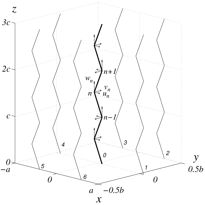
Figure 1: Schematic presentation of monoclinic structure of crystalline PE. The considered chain (curve 0) with local coordinates and 6 neighbor chains (curves 1-6) are shown.

2 Description of the model

Because in numerical study we deal not only with planar motion of the chain but take also into account the spatial movement and interchain interactions, three-dimensional hamiltonian is presented below.

It is suggested that the zig-zag initial structure of PE macromolecule is directed along the $z$-axis in plane ($x,z$), while $y$-axis is perpendicular to the plane $(x,z)$ so that $(x,y,z)$ is the positive global reference of the problem, $\theta_{0}$ being the angle of the zigzag chain.

Initial coordinates of the $n$-th mass of the chain are :

$$z_{n}^{0}=nl_{z},~{}~{}~{}x_{n}^{0}=(-1)^{n+1}l_{x}/2,$$ (1)

where $l_{z}=s\rho_{0}$ and $l_{x}=c\rho_{0}$ [$s=\sin(\theta_{0}/2)$, $c=\cos(\theta_{0}/2)$) are longitudinal and transversal dimensions of the initial zigzag chain. We use approximation of ”united atoms” because relative motions of hydrogen atoms are non-significant when dealing with backbone deformation predominantly. So the magnitude of every mass is supposed to be equal to 14 a.u. It is convenient to introduce the relative coordinates

$$u_{n}=x_{n}-x_{n}^{0},~{}~{}~{}w_{n}=z_{n}-z_{n}^{0},$$ (2)

where $w_{n}$, $u_{n}$, $v_{n}$ determine the longitudinal, transversal and out-of-plane displacements of the $n$-th mass from its equilibrium state. Let us denote by $\rho_{n}$ and $\theta_{n}$ the current length of the valence bond and current valence angle respectively. We introduce also $\phi_{n}$ as the angle between $d_{n-1}$ and the plane generated by $d_{n}$ and $d_{n+1}$ (conformation angle).

The dynamics of the chain is governed by the following hamiltonian function of the chain [24]:

$$H = \sum_{n=-\infty}^{+\infty}\{\frac{1}{2}m(\dot{u}_{n}^{2}+\dot{v}_{n}^{2}+\dot{w}_{n}^{2})$$ (3)

$$+[p_{1}+p_{2}\cos(\phi_{n})+p_{3}\cos(3\phi_{n})]$$

$$+\frac{1}{2}\Lambda[\cos(\theta_{n})-\cos(\theta_{0})]^{2}$$

$$+{\cal D}[1-e^{-q(\rho_{n}-\rho_{0})}]^{2}\}+Z(u_{n},v_{n},w_{n})$$

where dots denote the time derivation, $\Lambda$ and ${\cal D}$ correspond to energies of valence angles and valence bonds respectively, and the last term the energy of interaction of the n^th unit with six neighboring chains (substrate potential). Parameters $p_{1},p_{2},p_{3}$ satisfy conditions $p_{1}=p_{2}+p_{3}$, $p_{2},p_{3}>0$, so that undeformed state corresponds to $\phi_{n}=\pi$. Let us set $k_{1}=2{\cal D}q^{2}$ and $k_{2}=\Lambda\sin^{2}\theta_{0}$. Then

$$\rho_{n}^{2}=(u_{n+1}-u_{n}-l_{x})^{2}+(v_{n+1}-v_{n})^{2}+(w_{n+1}-w_{n}+l_{z})^{2}.$$ (4)

We have also:

$$\cos\theta_{n} = (-a_{n-1,1}a_{n,1}-a_{n-1,2}a_{n,2}$$ (5)

$$-a_{n-1,3}a_{n,3})/\rho_{n}\rho_{n-1},$$

$$\cos\phi_{n} = (b_{n,1}b_{n+1,1}+b_{n,2}b_{n+1,2}$$ (6)

$$+b_{n,3}b_{n+1,3})/\beta_{n}\beta_{n+1},$$

where

$$b_{n,1} = a_{n-1,2}a_{n,3}-a_{n,2}a_{n-1,3},$$

$$b_{n,2} = a_{n-1,3}a_{n,1}-a_{n,3}a_{n-1,1},$$

$$b_{n,3} = a_{n-1,1}a_{n,2}-a_{n,1}a_{n-1,2}$$

are related to inner product vector coordinates, and $\beta_{n}=(b_{n,1}^{2}+b_{n,2}^{2}+b_{n,3}^{2})^{1/2}$ are norms of corresponding vectors with

$$a_{n,1} = u_{n+1}-u_{n}+l_{x},$$

$$a_{n,2} = v_{n+1}-v_{n},$$

$$a_{n,3} = w_{n+1}-w_{n}+l_{z},$$

$$\rho_{n} = (a_{n,1}^{2}+a_{n,2}^{2}+a_{n,3}^{2})^{1/2},$$

which are the vector coordinates. The substrate potential

$$Z(u,v,w)=\varepsilon_{w}\sin^{2}(\pi w/l_{z})+{1\over 2}K_{u}[1+\varepsilon_{u}\sin^{2}({{\pi w}\over{l_{z}}})]\{u-{1\over 2}l_{x}[1-\cos(({{\pi w}\over{l_{z}}})]\}^{2}+{1\over 2}K_{v}[1+\varepsilon_{v}\sin^{2}({{\pi w}\over{l_{z}}})]v^{2},$$

where $\varepsilon_{u}=0.0674265$ kJ/mol, $\varepsilon_{v}=0.0418353$ kJ/mol, $\varepsilon_{w}=0.1490124$ kJ/mol, $K_{u}=2.169513$ kJ/ $\AA$ mol², $K_{v}=13.683865$ kJ/ $\AA$ mol².

3 Planar motion of zigzag chain

We consider further analytically only in-plane dynamics of zigzag. In both linear and nonlinear problems such a dynamics can be fully separated from out-of-plane motion. Therefore, general Hamiltonian can be simplified and one can obtain in both physically and geometrically nonlinear approach:

$$H = \sum_{n=-\infty}^{+\infty}\frac{1}{2}m(\dot{u}_{n}^{2}+\dot{w}_{n}^{2})\mbox{ terms up to order 4 from}$$ (7)

$$\Biggl{\{}\sum_{n=-\infty}^{+\infty}\frac{1}{2}\Lambda[\cos(\theta_{n})-\cos(\theta_{0})]^{2}$$

$$+\sum_{n=-\infty}^{+\infty}{\cal D}[1-e^{-q(\rho_{n}-\rho_{0})}]^{2}\Biggr{\}}$$

There are two systems of parameters describing PE macromolecules which are supposed in [19] and [20] respectively which differ by value of parameter $k_{2}$ ($k_{2}/\sin^{2}\theta_{0}=130.1$ kJ/mol in [19] and 529 kJ/mol in [19]). We will consider both systems supposing [18, 19] that $k_{1}/q^{2}=334.7$ kJ/mol, $q=19.1$ nm^-1, $\theta_{0}=113^{\circ}$, $\rho_{0}=1.54$ Å  so that $\delta=k_{2}/k_{1}\rho_{0}^{2}=0.019$ [19] or 0.078 [20].

The deformations are presented by their power expansions including the terms of first and second order with respect to displacements:

$$\Delta\rho_{n} = \rho_{n}-\rho_{0}=$$ (8)

$$(u_{n}-u_{n+1})c+(w_{n+1}-w_{n})s+{1\over{2\rho_{0}}}((u_{n}-u_{n+1})c+(w_{n+1}-w_{n})s)^{2}+\dots,$$

$$\Delta\theta_{n} = \theta_{n}-\theta_{0}=$$ (9)

$$\frac{s}{\rho_{0}}(2u_{n}-u_{n-1}-u_{n+1})+\frac{c}{\rho_{0}}(w_{n-1}-w_{n+1})$$

$$+\frac{cs}{\rho_{0}^{2}}[(u_{n}-u_{n+1})^{2}+(u_{n}-u_{n-1})^{2}-(w_{n}-w_{n+1})^{2}-(w_{n}-w_{n-1})^{2}]$$

$$+\frac{c^{2}-s^{2}}{\rho_{0}^{2}}[(w_{n}-w_{n-1})(u_{n}-u_{n-1})+(w_{n+1}-w_{n})(u_{n}-u_{n+1})]+...$$

Equations of motion are obtain in the form:

$$m{\displaystyle{{{\partial^{2}}\over{\partial t^{2}}}}}{u}_{n}=-\frac{\partial H}{\partial u_{n}},~{}~{}~{}m{\displaystyle{{{\partial^{2}}\over{\partial t^{2}}}}}{w}_{n}=-\frac{\partial H}{\partial w_{n}}$$ (10)

for the $n$th particle. Linearized equations are given by

$$m{\displaystyle{{{\partial^{2}}\over{\partial t^{2}}}}}u_{n} + k_{1}sc(w_{n+1}-w_{n-1})+k_{1}c^{2}(2u_{n}-u_{n-1}-u_{n+1})$$ (11)

$$+ k_{2}cs(w_{n-2}+2w_{n-1}-2w_{n+1}-w_{n+2})/\rho_{0}^{2}$$

$$+ k_{2}s^{2}(u_{n-2}-4u_{n-1}+6u_{n}-4u_{n+1}+u_{n+2})/\rho_{0}^{2}=0$$

$$m{\displaystyle{{{\partial^{2}}\over{\partial t^{2}}}}}w_{n} - k_{1}s^{2}(w_{n+1}-2w_{n}+w_{n-1})+k_{1}sc(u_{n+1}-u_{n-1})$$ (12)

$$- k_{2}c^{2}(w_{n-2}-2w_{n}+w_{n+2})/\rho_{0}^{2}$$

$$+ k_{2}s^{2}(-u_{n-2}+2u_{n-1}-2u_{n+1}+u_{n+2})/\rho_{0}^{2}=0$$

4 Dispersion relations

The linear dispersion curves have well known form (see, e.g. [24]), which is described by relation :

$$\omega^{2}(k)=f(k)=\omega_{0}^{2}(k)\pm\sqrt{\omega_{0}^{4}(k)-\omega_{1}^{4}(k)}$$ (13)

where

$$\omega_{0}^{2}(k) = C_{1}(1-\cos\theta_{0}\cos k)$$ (14)

$$+2C_{2}(1-\cos k)(1+\cos k\cos\theta_{0}),$$

$$\omega_{1}^{4}(k) = 8C_{1}C_{2}(1-\cos k)\sin^{2}k.$$

Here, $C_{1}=k_{1}/m$, $C_{2}=k_{2}/m\rho_{0}^{2}$, $k=\tilde{k}l_{z}$, $\tilde{k}$ is wave number. Signs ”minus” and ”plus” correspond to acoustic and optic branches respectively. We consider further the optic branch only. Corresponding asymptotic representations of the linear frequencies can be presented as follows in the vicinity of arbitrary wave number $k^{\star}$:

$$\omega^{2}(k)=\Omega^{2}+\nu(k-k^{\star})+\mu(k-k^{\star})^{2}+\dots=f(k),$$ (15)

with

$$\Omega^{2} = 2C_{1}[1-\cos(\theta_{0})\cos(k^{\star})]-{{4C_{2}\cos^{2}(k^{\star})\sin^{2}(\theta_{0})}\over{1-\cos(\theta_{0})\cos(k^{\star})}}[1-\cos(k^{\star})],$$

$$\nu = 2C_{1}\sin(k^{\star})\cos(\theta_{0})$$ (16)

$$+{{2C_{2}\sin(2k^{\star})\sin^{2}(\theta_{0})}\over{(1-\cos(\theta_{0})\cos(k^{\star}))^{2}}}[(1-\cos(k^{\star}))(2\cos(k^{\star})-1)+\cos(\theta_{0})\cos(k^{\star})-1],$$

$$\mu = C_{1}\cos(\theta_{0})\cos(k^{\star})+{{C_{2}\sin^{2}(\theta_{0})}\over{(\cos(\theta_{0})\cos(k^{\star})-1)^{3}}}[-4+12\cos(k^{\star})$$

$$+4\cos^{2}(k^{\star})(2-3\cos(\theta_{0}))-2\cos^{3}(k^{\star})(-2\cos^{2}(\theta_{0})+3\cos(\theta_{0})+9)$$

$$+2\cos^{4}(k^{\star})\cos(\theta_{0})(\cos(\theta_{0})+11)-8\cos^{5}(k^{\star})\cos^{2}(\theta_{0})].$$

Table 1 provides values of $\Omega^{2},\nu,\mu$ for some particular $k$.

Table 1: Values of $\Omega^{2},\nu,\mu$ for some particular $k$.

$k$	$\Omega^{2}$	$\nu$	$\mu$
$0$	$4s^{2}C_{1}$	0	$C_{1}(\cos(\theta_{0})+4c^{2}\delta)$
$\pi$	$4C_{1}(c^{2}+4s^{2}\delta)$	0	$-C_{1}\displaystyle{{{\cos(\theta_{0})c^{2}+20c^{2}s^{2}\delta}\over{c^{2}+4s^{2}\delta}}}$
$\pi/2$	$2C_{1}$	$2C_{1}\cos(\theta_{0})$	$\displaystyle{4C_{1}C_{2}{{\sin^{2}(\theta_{0})}\over{C1-2C_{2}}}}$

Analysis of general expressions of dispersion curves in application to realistic values of chain parameters reveals two types of behavior. The corresponding plots of dispersion curves are presented in Fig. 2.

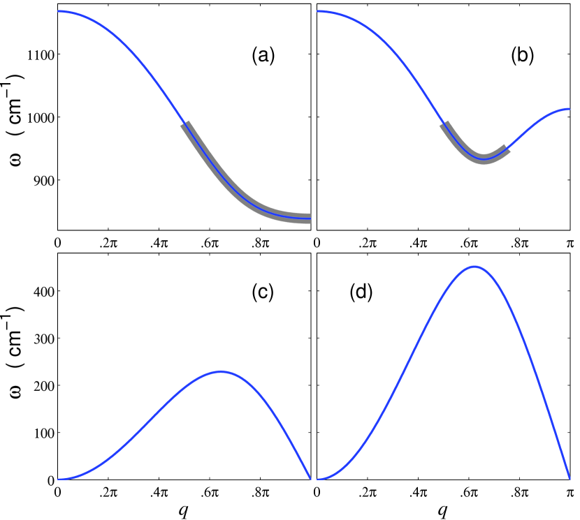
Figure 2: Dispersion curves: optic (a, b) and acoustic (c, d) branches for $\delta=0.019$ (a, c) and for $\delta=0.078$ (b, d) (parameter $C_{2}=\delta C_{1}$). Thick part of the dispersion curves correspond to possible existence of the breathers.

Let us introduce $C_{2}=\delta C_{1}$. The signs of numerical values of optic dispersion curves curvature $\cal{H}$ are:

• $\delta=0.019$, ${\cal H}(0)<0$, ${\cal H}(\pi)>0$, ${\cal H}(\pi/2)<0$,

• $\delta=0.078$, ${\cal H}(0)<0$, ${\cal H}(\pi)<0$, ${\cal H}(\pi/2)>0$.

We can see that for $k\approx 0$ curvature is negative in both cases. For $k\approx\pi$, $k\approx\pi/2$ it could be both positive or negative depending on the magnitude of $\delta$. The signs of the curvature determine as we will see the signs of second spatial derivatives in final continuum equations of motion. Let us define $k_{0}\in]0,\pi[$ so that the corresponding coefficient $\nu$ is equal to zero: $f^{\prime}(k_{0})=0$ ($k_{0}$ is defined only for $\delta=0.078$, because for $\delta=0.019$ the value $\nu=0$ at boundaries of wave number diapason only).

5 Introduction of modulating functions

In this section we introduce slow modulating functions in order to extend analysis based on normal modes that can be done for linearized equations to the nonlinear case. So we consider equations for $u_{n},w_{n}$ both with modulating continuous space functions $W,{\tilde{W}}$ expanded close to arbitrary n^th particle:

$$u_{n+m}=\cos(mk)[U+m\epsilon{{\partial U}\over{\partial\xi}}+{1\over 2}m^{2}\epsilon^{2}{{\partial^{2}U}\over{\partial\xi^{2}}}]+\sin(mk)[{\tilde{U}}+m\epsilon{{\partial{\tilde{U}}}\over{\partial\xi}}+{1\over 2}m^{2}\epsilon^{2}{{\partial^{2}{\tilde{U}}}\over{\partial\xi^{2}}}]+\dots$$ (17)

$$w_{n+m}=\cos(mk)[W+m\epsilon{{\partial W}\over{\partial\xi}}+{1\over 2}m^{2}\epsilon^{2}{{\partial^{2}W}\over{\partial\xi^{2}}}]+\sin(mk)[{\tilde{W}}+m\epsilon{{\partial{\tilde{W}}}\over{\partial\xi}}+{1\over 2}m^{2}\epsilon^{2}{{\partial^{2}{\tilde{W}}}\over{\partial\xi^{2}}}]+\dots$$ (18)

where $\epsilon$ is a small parameter characterizing distance between particles in the units $\xi=\varepsilon^{-1}z/l_{z}$, $z$ being dimensional distance.

In the same spirit, we consider equations for $u_{n+1},w_{n+1}$, both with the modulating functions expanded close to the ${n+1}^{th}$ particle (i.e. now with $u_{n+1}={\tilde{U}}$, $w_{n+1}={\tilde{W}}$):

$$u_{n+1+m}=\sin(-mk)[U+m\epsilon{{\partial U}\over{\partial\xi}}+{1\over 2}m^{2}\epsilon^{2}{{\partial^{2}U}\over{\partial\xi^{2}}}]+\cos(mk)[{\tilde{U}}+m\epsilon{{\partial{\tilde{U}}}\over{\partial\xi}}+{1\over 2}m^{2}\epsilon^{2}{{\partial^{2}{\tilde{U}}}\over{\partial\xi^{2}}}]+\dots$$ (19)

$$w_{n+1+m}=\sin(-mk)[W+m\epsilon{{\partial W}\over{\partial\xi}}+{1\over 2}m^{2}\epsilon^{2}{{\partial^{2}W}\over{\partial\xi^{2}}}]+\cos(mk)[{\tilde{W}}+m\epsilon{{\partial{\tilde{W}}}\over{\partial\xi}}+{1\over 2}m^{2}\epsilon^{2}{{\partial^{2}{\tilde{W}}}\over{\partial\xi^{2}}}]+\dots$$ (20)

Necessity to consider the expansions in the vicinities of two points is caused by twice degeneration of linear normal normal modes spectrum (except the boundary values of wave number). By substituting modulating functions in the linearized equations for $u_{n}$, $u_{n+1}$, $w_{n}$, $w_{n+1}$ (11), (12), one obtains 4 partial differential equations in the general case that take into account linear part of the equations for modulations of normal modes. Linearized equations for modulations of normal modes have to be in accordance with dispersion relations presented above. We present them below for special case $k=\pi/2$.

$$\matrix{\displaystyle{{{\partial^{2}U}\over{\partial t^{2}}}-2(C_{1}c^{2}+4C_{2}s^{2})\epsilon{{\partial\tilde{U}}\over{\partial\xi}}-4csC_{2}\epsilon{{\partial W}\over{\partial\xi}}-4C_{2}s^{2}\epsilon^{2}{{\partial^{2}U}\over{\partial\xi^{2}}}}\cr\quad\cr\displaystyle{+sc(2C_{2}+C_{1})\epsilon^{2}{{\partial^{2}{\tilde{W}}}\over{\partial\xi^{2}}}+2(c^{2}C_{1}+2s^{2}C_{2})U+2sc(2C_{2}-C_{1}){\tilde{W}}=0,}\cr}$$ (21)

$$\matrix{\displaystyle{{{\partial^{2}W}\over{\partial t^{2}}}-2C_{1}s^{2}\epsilon{{\partial\tilde{W}}\over{\partial\xi}}+4csC_{2}\epsilon{{\partial U}\over{\partial\xi}}+4C_{2}c^{2}\epsilon^{2}{{\partial^{2}W}\over{\partial\xi^{2}}}}\cr\quad\cr\displaystyle{+sc(2C_{2}-C_{1})\epsilon^{2}{{\partial^{2}{\tilde{U}}}\over{\partial\xi^{2}}}+2(s^{2}C_{1}+2c^{2}C_{2})W+2sc(2C_{2}-C_{1}){\tilde{U}}=0,}\cr}$$ (22)

$$\matrix{\displaystyle{{{\partial^{2}{\tilde{U}}}\over{\partial t^{2}}}+2(C_{1}c^{2}+4C_{2}s^{2})\epsilon{{\partial U}\over{\partial\xi}}+4scC_{2}\epsilon{{\partial{\tilde{W}}}\over{\partial\xi}}-4C_{2}s^{2}\epsilon^{2}{{\partial^{2}{\tilde{U}}}\over{\partial\xi^{2}}}}\cr\quad\cr\displaystyle{+sc(2C_{2}-C_{1})\epsilon^{2}{{\partial^{2}W}\over{\partial\xi^{2}}}+2(c^{2}C_{1}+2s^{2}C_{2}){\tilde{U}}+2sc(2C_{2}-C_{1})W}=0,\cr}$$ (23)

$$\matrix{\displaystyle{{{\partial^{2}{\tilde{W}}}\over{\partial t^{2}}}+2C_{1}s^{2}\epsilon{{\partial W}\over{\partial\xi}}-4csC_{2}\epsilon{{\partial{\tilde{U}}}\over{\partial\xi}}+4C_{2}c^{2}\epsilon^{2}{{\partial^{2}{\tilde{W}}}\over{\partial\xi^{2}}}}\cr\quad\cr\displaystyle{+sc(2C_{2}-C_{1})\epsilon^{2}{{\partial^{2}U}\over{\partial\xi^{2}}}+2(s^{2}C_{1}+2c^{2}C_{2}){\tilde{W}}+2sc(2C_{2}-C_{1})U=0.}\cr}$$ (24)

Then we introduce operator approximation for ${\displaystyle{{{\partial^{2}}\over{\partial t^{2}}}}}u_{n}$ and ${\displaystyle{{{\partial^{2}}\over{\partial t^{2}}}}}u_{n+1}$ in corresponding equations using previous Taylor expansions and expansion of dispersion relation according to

$$\left\{\matrix{\displaystyle{{\displaystyle{{{\partial^{2}}\over{\partial t^{2}}}}}u_{n}\simeq-\omega^{2}U=-\Omega^{2}U+\nu\epsilon{{\partial{\tilde{U}}}\over{\partial\xi}}+\mu\epsilon^{2}{{\partial^{2}U}\over{\partial\xi^{2}}}\dots}\cr\displaystyle{{\displaystyle{{{\partial^{2}}\over{\partial t^{2}}}}}u_{n+1}\simeq-\omega^{2}{\tilde{U}}=-\Omega^{2}{\tilde{U}}-\nu\epsilon{{\partial U}\over{\partial\xi}}+\mu\epsilon^{2}{{\partial^{2}{\tilde{U}}}\over{\partial\xi^{2}}}+\dots}\cr}\right.$$ (25)

Substitution of (23), (24) into starting nonlinear equation (9) leads to four nonlinear partial differential equations (NPDE) with respect to functions $W$, $\tilde{W}$, $U$, $\tilde{U}$. To reduce the order of this system one can express the functions $U$, $\tilde{U}$ via $W$, $\tilde{W}$ using the equations for $U$ and $\tilde{U}$, and taking into account the terms up to third degree. As this takes place, we have to replace the nonlinear terms with respect $U$, $\tilde{U}$ by their expressions via $W$, $\tilde{W}$ obtained from (21), (23), (24). Then NPDE for $U$ and $\tilde{U}$ provide two independent linear relations relative these functions that can be solved to obtain $U$ and ${\tilde{U}}$ versus $W$ and ${\tilde{W}}$. Indeed truncation of the full NPDE at order 3 are used. At this step, one can notice that for $k=\pi/2$ or $k=k_{0}$ displacements $u_{n}$ and $w_{n}$ are of same order: we have longitudinal and transversal motions. If measuring the length in units $l_{z}$ we have $k\sim\pi/2:~{}u_{n}\sim w_{n}$. In strongly coupled general case, the relations can be written as:

$$U=A_{1}W+A_{2}{\tilde{W}}+{\cal F}_{12}(W,{\tilde{W}})+{\cal F}_{13}(W,{\tilde{W}})+A_{3}\epsilon{{\partial W}\over{\partial\xi}}+A_{4}\epsilon{{\partial{\tilde{W}}}\over{\partial\xi}}+A_{5}\epsilon^{2}{{\partial^{2}W}\over{\partial\xi^{2}}}+A_{6}\epsilon^{2}{{\partial^{2}{\tilde{W}}}\over{\partial\xi^{2}}}+\dots,$$ (26)

$${\tilde{U}}=B_{1}W+B_{2}{\tilde{W}}+{\cal F}_{22}(W,{\tilde{W}})+{\cal F}_{23}(W,{\tilde{W}})+B_{3}\epsilon{{\partial W}\over{\partial\xi}}+B_{4}\epsilon{{\partial{\tilde{W}}}\over{\partial\xi}}+B_{5}\epsilon^{2}{{\partial^{2}W}\over{\partial\xi^{2}}}+B_{6}\epsilon^{2}{{\partial^{2}{\tilde{W}}}\over{\partial\xi^{2}}}+\dots,$$ (27)

with ${\cal F}_{ij},i=1,2$ of degree $j$ in $W,{\tilde{W}}$. $A_{k},B_{k}$, $k=1,\dots,6$ are given constants. For example, if $k=\pi/2$, one has:

$$\left\{\matrix{\displaystyle{A_{1}=0,A_{2}=-{c\over s},{\cal F}_{12}(W,{\tilde{W}})=D(W^{2}+{\tilde{W}}^{2}),}\cr\quad\cr\displaystyle{B_{2}=0,B_{1}=-{c\over s},{\cal F}_{22}(W,{\tilde{W}})=-D(W^{2}+{\tilde{W}}^{2}),}\cr\quad\cr\displaystyle{D={{3cq\rho_{0}C_{1}}\over{2s^{4}(C_{1}-2C_{2})}}}\cr}\right.$$ (28)

For $k=0$ or $k=\pi$, degeneracy of order occurs: $u$ or $w$ displacements dominate. We have:

$$\matrix{k\sim 0:~{}u_{n}\sim kw_{n}\sim\varepsilon w_{n},\hbox{ we suppose that }k\sim\varepsilon<<1\cr k\sim\pi:~{}w_{n}\sim(\pi-k)u_{n}\sim\varepsilon u_{n}.\cr}$$

Then modulating functions introduced in equations for $u_{n}$ and $w_{n}$ provide only 2 NPDE. In these two particular cases, one needs only to consider equation for $u_{n}$ (or respectively $w_{n}$). The relations, connecting $u_{n}$ and $w_{n}$ are obtained in the form

$$u_{n}=U=\varepsilon\left[\frac{c}{s}\frac{\partial W}{\partial\xi}+\frac{c}{\rho_{0}s^{2}}(2-3c^{2}+3s^{2}\rho_{0}q-8\delta s^{2})W^{2}\right]+\dots$$ (29)

for $k=0$ and

$$w_{n}=W=-\frac{sc}{2}\frac{1-4\delta}{4\delta s^{2}+c^{2}}\varepsilon\frac{\partial U}{\partial\xi}+\dots$$ (30)

for $k=\pi$.

6 Nonlinear partial equations

Let us introduce new non-dimensional time by relation $\tau=\Omega t$, where $\Omega$ is linear frequency for considered normal mode. After substitution of the expressions of the displacements via modulating functions into equations for $w_{n}$ and $w_{n+1}$, one can obtain corresponding nonlinear partial differential equations for modulating functions in the form:

$$\matrix{\displaystyle{{{\partial^{2}W}\over{\partial\tau^{2}}}+{{f^{\prime}(k)}\over\Omega^{2}}\epsilon{{\partial\tilde{W}}\over{\partial\xi}}-{{f^{\prime\prime}(k)}\over\Omega^{2}}\epsilon^{2}{{\partial^{2}W}\over{\partial\xi^{2}}}+W}\cr\quad\cr\displaystyle{+{1\over{\Omega^{2}}}[D_{1}W^{2}+D_{2}W{\tilde{W}}+D_{3}{\tilde{W}}^{2}+D_{4}W^{3}+D_{5}W^{2}{\tilde{W}}+D_{6}W{\tilde{W}}^{2}+D_{7}{\tilde{W}}^{3}]+\dots=0,}\cr}$$ (31)

$$\matrix{\displaystyle{{{\partial^{2}{\tilde{W}}}\over{\partial\tau^{2}}}-{{f^{\prime}(k)}\over\Omega^{2}}\epsilon{{\partial W}\over{\partial\xi}}-{{f^{\prime\prime}(k)}\over\Omega^{2}}\epsilon^{2}{{\partial^{2}{\tilde{W}}}\over{\partial\xi^{2}}}+{\tilde{W}}}\cr\quad\cr\displaystyle{+{1\over{\Omega^{2}}}[-D_{3}W^{2}-D_{2}W{\tilde{W}}-D_{1}{\tilde{W}}^{2}+D_{7}W^{3}+D_{6}W^{2}{\tilde{W}}+D_{5}W{\tilde{W}}^{2}+D_{4}{\tilde{W}}^{3}]+\dots=0,}\cr}$$ (32)

where $D_{j}$,$j=1,\dots,7$ are constants depending on $C_{1},C_{2},\rho_{0},q,\theta_{0}$. For $k=\pi/2$, the expressions are given in table 2. They are not given for the general case because of size of expressions. Numerical values for $K=K_{0}$, in re-scaled nondimensional form corresponding to $\varepsilon=0.05$ are given in table 2.

Table 2: Values of constants $D_{j}$, $j=1,\dots,7$ for $k=\pi/2$ and numerical values for $k=k_{0}$, corresponding to $\varepsilon=0.05$.

$j$	$k=\pi/2$	$k=k_{0}$
$1$	$\displaystyle{{{(C_{1}-2C_{2})Dcs}/{C_{1}}}}$	2.25
$2$	0	-5.74
$3$	$\displaystyle{{{(C_{1}-2C_{2})Dcs}/{C_{1}}}}$	2.57
$4$	-$\displaystyle{{{D(3C_{1}q\rho_{0}+C_{1}-2C_{2})}/{C_{1}}}}$	1.89
$5$	$\displaystyle{{{D(3C_{1}q\rho_{0}+C_{1}-2C_{2})}/{C_{1}}}}$	-1.14
$6$	-$\displaystyle{{{D(3C_{1}q\rho_{0}+C_{1}-2C_{2})}/{C_{1}}}}$	2.42
$7$	$\displaystyle{{{D(3C_{1}q\rho_{0}+C_{1}-2C_{2})}/{C_{1}}}}$	-1.14

Again, degeneracy of cases $k=0$ or $k=\pi$ leads to only one equation obtained from equation for $w_{n}$ as:

$$\left\{\matrix{\displaystyle{{{\partial^{2}\tilde{W}}\over{\partial\tau^{2}}}-\lambda_{1}\varepsilon^{2}{{\partial^{2}\tilde{W}}\over{\partial\xi^{2}}}+\tilde{W}}\displaystyle{+\alpha_{2}{\tilde{W}}^{3}=0,}\cr\quad\cr\displaystyle{\lambda_{1}={{C_{1}\cos(\theta_{0})+4c^{2}C_{2}}\over{4s^{2}C_{1}}},}\cr\quad\cr\displaystyle{\alpha_{2}={1\over{\rho_{0}^{2}}}[2(5c^{2}-4)c^{2}/s^{2}+{{14}\over 3}\rho_{0}^{2}q^{2}s^{2}-12\rho_{0}qc^{2}+32\delta c^{2}],}\cr}\right.$$ (33)

for $k=0$ and

$$\left\{\matrix{\displaystyle{{{\partial^{2}\tilde{U}}\over{\partial\tau^{2}}}-\lambda_{2}\epsilon^{2}{{\partial^{2}\tilde{U}}\over{\partial\xi^{2}}}+\tilde{U}+\alpha_{1}{\tilde{U}}^{2}+\alpha_{2}{\tilde{U}}^{3}=0,}\cr\quad\cr\displaystyle{\lambda_{2}=-{{C_{1}\cos(\theta_{0})c^{2}+20c^{2}s^{2}C_{2}}\over{4(c^{2}+4s^{2}\delta)^{2}}},}\cr\quad\cr\displaystyle{\alpha_{1}={3\over c}{{c^{2}(s^{2}-c^{2}q\rho_{0})+4s^{2}(1-4c^{2})\delta}\over{c^{2}+4s^{2}\delta}},}\cr\quad\cr\displaystyle{\alpha_{2}=-{{2[3c^{2}s^{2}(5c^{2}-1)+18c^{4}s^{2}q\rho_{0}-7c^{6}q^{2}\rho_{0}^{2}-12\delta s^{2}(48c^{4}-24c^{2}+1)]}\over{3c^{2}(c^{2}+4s^{2}\delta)}},}\cr}\right.$$ (34)

for $k=\pi$. In the last NPDE, nonlinear terms involving spatial derivatives can be neglected because they are of higher orders by $\epsilon$.

All these NPDE have been given in dimensional form. They could be re-scaled according to physical orders of the different variables (e.g. replacing the variables $U,{\tilde{U}},W,{\tilde{W}}$ by $\varepsilon\rho_{0}U$, $\varepsilon\rho_{0}{\tilde{U}}$, $\varepsilon\rho_{0}W$, $\varepsilon\rho_{0}\tilde{W}$). This has been done for numerical applications in the cases $k\approx 0$, $k\approx\pi$ and $k=k_{0}$ below. Such re-scaling makes the orders of nonlinear terms to be similar to those of the terms containing second spatial derivatives.

7 Transition to complex variables

The NPDE of previous section can be written under first order by time if setting

$$\matrix{k\sim 0,~{}~{}\Psi(\xi,\tau)=(W^{\prime}+i{W}),~{}~{}\Psi^{\star}(\xi,\tau)=(W^{\prime}-i{W}),\cr\quad\cr k\sim\pi,~{}~{}\Psi(\xi,\tau)=(U^{\prime}+i{U}),~{}~{}\Psi^{\star}(\xi,\tau)=(U^{\prime}-iU),\cr\quad\cr k\sim\pi/2\hbox{ or }k_{0},~{}~{}\left\{\matrix{\Psi_{1}(\xi,\tau)=(W^{\prime}+iW),~{}~{}\Psi_{1}^{\star}(\xi,\tau)=(W^{\prime}-iW),\cr\quad\cr\Psi_{2}(\xi,\tau)=({\tilde{W}}^{\prime}+i\tilde{W}),~{}~{}\Psi_{2}^{\star}(\xi,\tau)=({\tilde{W}}^{\prime}-i\tilde{W}).\cr}\right.\cr}$$ (35)

We obtain two NPDE, for $k=0$:

$$\left\{\matrix{\displaystyle{-i{{\partial\Psi}\over{\partial\tau}}=\Psi-{\lambda_{1}\over 2}\epsilon^{2}{{\partial^{2}}\over{\partial\xi^{2}}}(\Psi-\Psi^{\star})-{\alpha_{2}\over 8}(\Psi-\Psi^{\star})^{3}+\dots}\cr\quad\cr\hbox{ Conjugate equation },\cr}\right.$$ (36)

and $k=\pi$ :

$$\left\{\matrix{\displaystyle{-i{{\partial\Psi}\over{\partial\tau}}=\Psi-{\lambda_{2}\over 2}\epsilon^{2}{{\partial^{2}}\over{\partial\xi^{2}}}(\Psi-\Psi^{\star})-{i\alpha_{1}\over 4}(\Psi-\Psi^{\star})^{2}-{\alpha_{2}\over 8}(\Psi-\Psi^{\star})^{3}+\dots}\cr\quad\cr\hbox{ Conjugate equation },\cr}\right.$$ (37)

In general case one can obtain four NDPE, e.g. for $k=\pi/2$ they have linear part

$$\left\{\matrix{\displaystyle{-i{{\partial\Psi_{1}}\over{\partial\tau}}=\Psi_{1}+{{f^{\prime}(k)}\over{\Omega^{2}}}\epsilon{{\partial^{2}}\over{\partial\xi^{2}}}(\Psi_{2}-\Psi_{2}^{\star})-{{f"(k)}\over{\Omega^{2}}}\epsilon^{2}{{\partial^{2}}\over{\partial\xi^{2}}}(\Psi_{1}-\Psi_{1}^{\star}),}\cr\quad\cr\hbox{ Conjugate equation,}\cr\quad\cr\displaystyle{-i{{\partial\Psi_{2}}\over{\partial\tau}}=\Psi_{2}-{{f^{\prime}(k)}\over{\Omega^{2}}}\epsilon{{\partial^{2}}\over{\partial\xi^{2}}}(\Psi_{1}-\Psi_{1}^{\star})-{{f"(k)}\over{\Omega^{2}}}\epsilon^{2}{{\partial^{2}}\over{\partial\xi^{2}}}(\Psi_{2}-\Psi_{2}^{\star}),}\cr\quad\cr\hbox{Conjugate equation}.\cr}\right.$$ (38)

Let us introduce the changes of variables

$$\tau_{0}=\tau,~{}~{}\tau_{1}=\varepsilon\tau_{0},~{}~{}\tau_{2}=\varepsilon^{2}\tau_{0},\dots$$ (39)

Setting $\psi=\phi e^{i\tau}$ (for $k=0$, $\pi$) and $\psi_{j}=\phi_{j}e^{i\tau}$, $j=1,2$ (for $k=\pi/2$) we use farther the power expansions

$$\phi=\varepsilon(\phi_{0}+\varepsilon\phi_{1}+\varepsilon^{2}\phi_{2}+\dots)$$ (40)

and respectively

$$\phi_{j}=\varepsilon(\phi_{j0}+\varepsilon\phi_{j1}+\varepsilon^{2}\phi_{j2}+\dots)$$ (41)

Then we obtain at order $\varepsilon^{0}$ the relations:

$$k=0:~{}-i\displaystyle{{{\partial\phi_{0}}\over{\partial\tau_{0}}}=0,}$$ (42)

$$k=\pi:~{}-i\displaystyle{{{\partial\phi_{0}}\over{\partial\tau_{0}}}=0,}$$ (43)

$$k=k_{0}:~{}-i\displaystyle{{{\partial\phi_{10}}\over{\partial\tau_{0}}}=0},~{}~{}-i\displaystyle{{{\partial\phi_{20}}\over{\partial\tau_{0}}}=0,}$$ (44)

It means that for $k=0$, $\pi$, $\phi_{0}=\phi_{0}(\xi,\tau_{1},\tau_{2})$ and for $k=k_{0}$, $\phi_{1,0}=\phi_{1,0}(\xi,\tau_{1},\tau_{2})$, $\phi_{2,0}=\phi_{2,0}(\xi,\tau_{1},\tau_{2})$. For $k=\pi/2$ presence of first space derivatives lead to different problem.

At order $\varepsilon^{1}$ we have the equations

$$k=0,\pi:~{}\displaystyle{{{\partial\phi_{1}}\over{\partial\tau_{0}}}+{{\partial\phi_{0}}\over{\partial\tau_{1}}}=0,}$$ (45)

$$k=k_{0}:~{}\displaystyle{{{\partial\phi_{1,1}}\over{\partial\tau_{0}}}+{{\partial\phi_{1,0}}\over{\partial\tau_{1}}}=0,}$$ (46)

$$\frac{\partial\phi_{2,1}}{\partial\tau_{0}}+\frac{\partial\phi_{2,0}}{\partial\tau_{1}}=0$$ (47)

Conditions of absence of resonances lead to equations

$$k=0,~{}\pi:~{}~{}\displaystyle{{{\partial\phi_{0}}\over{\partial\tau_{1}}}=0,}$$ (48)

$$k=k_{0}:~{}~{}\displaystyle{{{\partial\phi_{1,0}}\over{\partial\tau_{1}}}=0,\frac{\phi_{2,0}}{\partial\tau_{1}}=0.}\hfill\qquad$$ (49)

Therefore $\phi_{0}=\phi_{0}(\xi,\tau_{2},\tau_{3},\dots)$ for $k=0,\pi$ as for the case $k=k_{0}$, we can write that $\phi_{j,0}=\phi_{j,0}(\xi,\tau_{2},\dots)$, $j=1,2$.

At order $\varepsilon^{2}$ the conditions of absence of resonance terms lead to final complex equations in main approach:

$$\matrix{\displaystyle{k=0,\pi:~{}~{}-i{{\partial\phi_{0}}\over{\partial\tau_{2}}}+\beta{{\partial^{2}\phi_{0}}\over{\partial\xi^{2}}}+\alpha\mid\phi_{0}\mid^{2}\phi_{0}=0,}\cr\displaystyle{k=0:\alpha=-{{3\alpha_{2}}\over{8}},\beta=\displaystyle{{\lambda_{1}/2}},}\cr\displaystyle{k=\pi,\alpha=-{{3\alpha_{2}}\over{8}}+{{5\alpha_{1}^{2}}\over{12}},\beta=\displaystyle{{\lambda_{2}/2}}}.\cr}$$ (50)

which is Nonlinear Schrödinger Equation (NSE) for $k=0$ and $k=\pi$ respectively. For $k=k_{0}$, the resonant equations have the general form:

$$\matrix{\displaystyle{-i{{\partial\phi_{1,0}}\over{\partial\tau_{2}}}-{\lambda_{2}\over 2}{{\partial^{2}\phi_{10}}\over{\partial\xi^{2}}}+P_{1}{\mid\phi_{10}\mid}^{2}\phi_{10}+P_{2}{\mid\phi_{10}\mid}^{2}\phi_{20}+P_{5}{\mid\phi_{20}\mid}^{2}\phi_{10}}\cr+P_{6}{\mid\phi_{20}\mid}^{2}\phi_{20}+P_{4}\phi_{10}^{2}\overline{\phi_{20}}+P_{5}\phi_{20}^{2}\overline{\phi_{10}}=0,\cr}$$ (51)

$$\matrix{\displaystyle{-i{{\partial\phi_{2,0}}\over{\partial\tau_{2}}}-{\lambda_{2}\over 2}{{\partial^{2}\phi_{20}}\over{\partial\xi^{2}}}+P_{1}{\mid\phi_{20}\mid}^{2}\phi_{20}+P_{2}{\mid\phi_{20}\mid}^{2}\phi_{10}+P_{5}{\mid\phi_{10}\mid}^{2}\phi_{20}}\cr+P_{6}{\mid\phi_{10}\mid}^{2}\phi_{10}+P_{4}\phi_{20}^{2}\overline{\phi_{10}}+P_{5}\phi_{10}^{2}\overline{\phi_{20}}=0=0.\cr}$$ (52)

with $P_{i},i=1,6$ constants derived from NPDE (31) and (32):

$$P_{1} = {3\over 8}D_{4}-{5\over{12}}D_{1}^{2}+{5\over{24}}D_{2}D_{3},$$

$$P_{2} = {1\over 8}D_{5}+{1\over{2}}D_{3}^{2}-{5\over{12}}D_{1}D_{2}+{1\over{12}}D_{2}^{2},$$

$$P_{3} = -{1\over{12}}D_{3}^{2}-{5\over{24}}D_{1}D_{2}+{1\over{8}}D_{2}^{2}+{1\over{8}}D_{5},$$

$$P_{4} = -{1\over{24}}D_{1}D_{2}-{1\over{8}}D_{2}^{2}+{1\over{12}}D_{1}D_{3}+{1\over{4}}D_{2}D_{3}+{1\over{8}}D_{6},$$

$$P_{5} = {3\over{8}}D_{7}-{5\over{24}}D_{2}D_{3}+{5\over{12}}D_{1}D_{3},$$

$$P_{6} = -{1\over{2}}D_{1}D_{3}-{1\over{12}}D_{2}^{2}+{1\over{4}}D_{6}+{1\over{6}}D_{2}D_{3}+{1\over{4}}D_{1}D_{2}.$$

8 Soliton-like solutions

As it is known, the type of soliton-like (breather) solutions depends strongly on relationship between the signs of constants $\alpha$ and $\beta$ of NSE. When these signs are similar, NSE admits the envelope solitons. In opposite case, NSE admits ”dark” solitons. From this point of view there is a significant difference between two systems of zigzag parameters introduced above.

For the case $k\sim 0$, and both values of $\delta$, the signs of $\alpha$ and $\beta$ are the same ($<0$) (see numerical values in table 3).

Table 3: Values of $\alpha,\beta$ versus $\delta$ for $k\sim 0$ or $\pi$.

$k$	$\delta$	$\alpha$	$\beta$
$0$	$0.019$	$0.053$	$-0.07$
$0$	$0.078$	$0.054$	$-0.05$
$\pi$	$0.019$	$0.035$	$0.021$
$\pi$	$0.078$	$0.033$	$-0.23$

For the case ($k\sim\pi$, $\delta=0.019$) the dispersion curve has a form similar to Figure 2 (a). In such a case the signs of $\alpha$ and $\beta$ are the same ($>0$). Then one can obtain the the envelope solitons (or breathers) as particular solutions:

$$\phi_{0}(\xi,\tau_{2}) = (2A/\alpha_{s})^{1/2}\exp(iv\xi/2\sqrt{\beta_{s}}+i\omega\tau_{2})$$ (53)

$$\times\mbox{sech}[A^{1/2}(\xi/\sqrt{\beta_{s}}+v\tau_{2})],$$

where $\omega=v^{2}/4-A$.

For the second system ($k\sim\pi$, $\delta=0.078$) the dispersion curve has a form similar to Figure 2 (b) (optic branch) and dark solitons exist.

In the case $k\sim k_{0}$, breather or dark soliton can exist near minimal frequency. This fact has been confirmed by computer simulation. Looking for particular solutions of the form $\phi_{2,0}=\gamma\phi_{10}$, we obtain only two possible values for $\gamma$: $\gamma=\pm 1$. The two coupled complex NPDE (51) and (52) can be reduced to only one Schrödinger equation of the form

$${-i{{\partial\phi_{1,0}}\over{\partial\tau_{2}}}+\beta{{\partial^{2}\phi_{10}}\over{\partial\xi^{2}}}+\alpha{\mid\phi_{10}\mid}^{2}\phi_{10}=0,}$$ (54)

with $\beta=-\lambda_{2}/2$, $\alpha=P_{1}+P_{4}+P_{6}+\gamma(P_{2}+P_{3}+P_{5})$. Numerical values are given in table 4. The breathers exist for $\gamma=1$ and dark solitons for $\gamma=-1$.

Table 4: Values of $\alpha,\beta$ versus $\delta$ for $k\sim k_{0}$, $\gamma=\pm 1$.

$\gamma$	$\delta$	$\alpha$	$\beta$
$+1$	$0.078$	$-0.010$	$0.28$
$-1$	$0.078$	$2.47$	$0.28$

9 Numerical simulations

To check the validity of assumption made in the analytical study, we have undertaken a numerical treatment of the breathers existence as well as their stability in free motions, under collisions and thermal perturbations.

While numerical modeling the breathers and their dynamics, we consider the following system of equations corresponding to Hamiltonian (3):

$$m{\displaystyle{{{\partial^{2}}\over{\partial t^{2}}}}}{u}_{n}=-\frac{\partial H}{\partial u_{n}},~{}~{}~{}m{\displaystyle{{{\partial^{2}}\over{\partial t^{2}}}}}{v}_{n}=-\frac{\partial H}{\partial v_{n}},~{}~{}~{}m{\displaystyle{{{\partial^{2}}\over{\partial t^{2}}}}}{w}_{n}=-\frac{\partial H}{\partial w_{n}}$$ (55)

for $n=1,2,...,N$.

We use initial conditions in agreement with approximate analytical solution. Because of small difference from exact solution, there will be a phonon radiation. For its absorption, the viscous friction is introduced at the end of the chain. As it was mentioned above, we deal with two systems of parameters for PE crystal. One of them is[19]:

$$m=14m_{p},~{}~{}p_{1}=8.37\mbox{kJ/mol},~{}~{}p_{2}=1.675\mbox{kJ/mol},$$

$$p_{3}=6.695\mbox{kJ/mol},~{}~{}\Lambda=130.122\mbox{kJ/mol},$$ (56)

$$\theta_{0}=113^{\circ},~{}~{}D=334.72\mbox{kJ/mol},$$

$$q=1.91\mbox{\AA}^{-1},~{}~{}\rho_{0}=1.53\mbox{\AA},$$

where $m_{p}$ is the proton mass. Second system of parameters which is used in [20] differs with more high value of parameter

$$\Lambda=529\mbox{kJ/mol}.$$ (57)

When using the first system of parameters (56), a geometric nonlinearity plays a crucial role in nonlinear dynamics of the PE chain. In the second case (57) a physical nonlinearity becomes more essential. Moreover, the dispersion curves for these two cases have different view. Respectively, the optic breathers will have different view and different regions of existence in parametric space (Fig. 2). Therefore we study numerically their properties for both systems of parameters.

Numerical integration of the equation of motion (55) has confirmed that in accordance with analytical study, the optic breathers exist for both systems of parameters (56) and (57) near low boundaries of the frequencies of optic phonons. Typical distribution of relative displacements in the localization region of planar breather is presented in Fig. 3, 4, 5. One can see that shift of frequency (see Fig. 3 and 4) leads to narrowing of breather. Analogous effect is achieved also when increasing the intensity of excitation – see Fig. 5. Characteristics of breathers for the systems of parameters (56), (57). are essentially different – see Fig. 6 and 7. In the localization regions of breathers the local change of valence angles is accompanied by local extension of zigzag (average values of relative longitudinal displacements $w_{n+1}-w_{n}$ are positive).

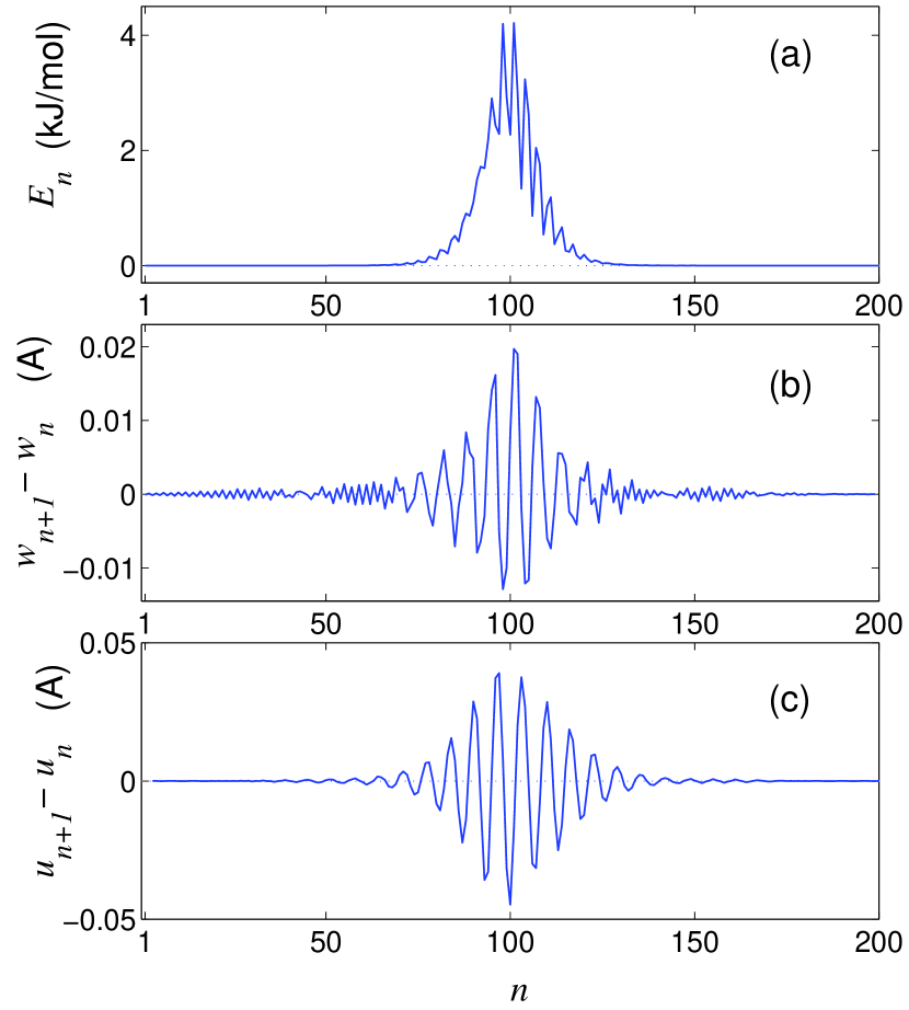
Figure 3: Optical breather in PE chain (parameter $\gamma=529$ kJ/mol). The distribution along the chain energy $E_{n}$ (a), longitudinal $w_{n+1}-w_{n}$ (b) and transversal $v_{n+1}-v_{n}$ (c) relative displacements of the chain segments is shown (breather energy $E=56.06$ kJ/mol, frequency $\omega=926$ cm^-1, velocity $s=0.15$ (1146 m/s).

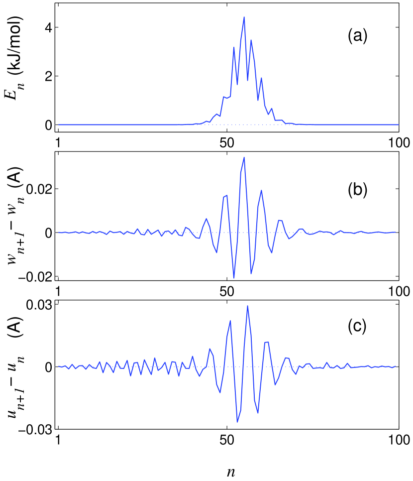
Figure 4: Optical breather in PE chain (parameter $\gamma=130.122$ kJ/mol). The distribution along the chain energy $E_{n}$ (a), longitudinal $w_{n+1}-w_{n}$ (b) and transversal $v_{n+1}-v_{n}$ (c) relative displacements of the chain segments is shown (breather energy $E=31.1$ kJ/mol, frequency $\omega=909$ cm^-1, velocity $s=0.48$ (3888 m/s).

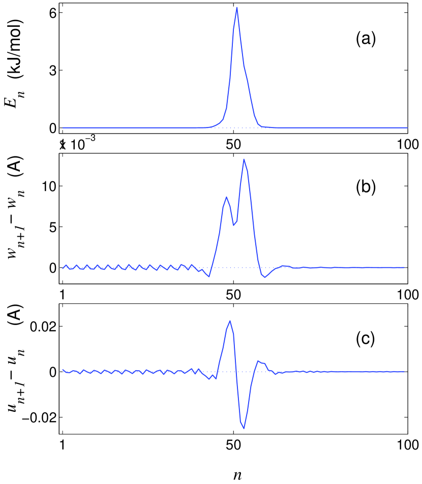
Figure 5: Optical breather in PE chain (parameter $\gamma=130.122$ kJ/mol). The distribution along the chain energy $E_{n}$ (a), longitudinal $w_{n+1}-w_{n}$ (b) and transversal $v_{n+1}-v_{n}$ (c) relative displacements of the chain segments is shown (breather energy $E=28.77$ kJ/mol, frequency $\omega=830$ cm^-1, velocity $s=0.16$ (1296 m/s).

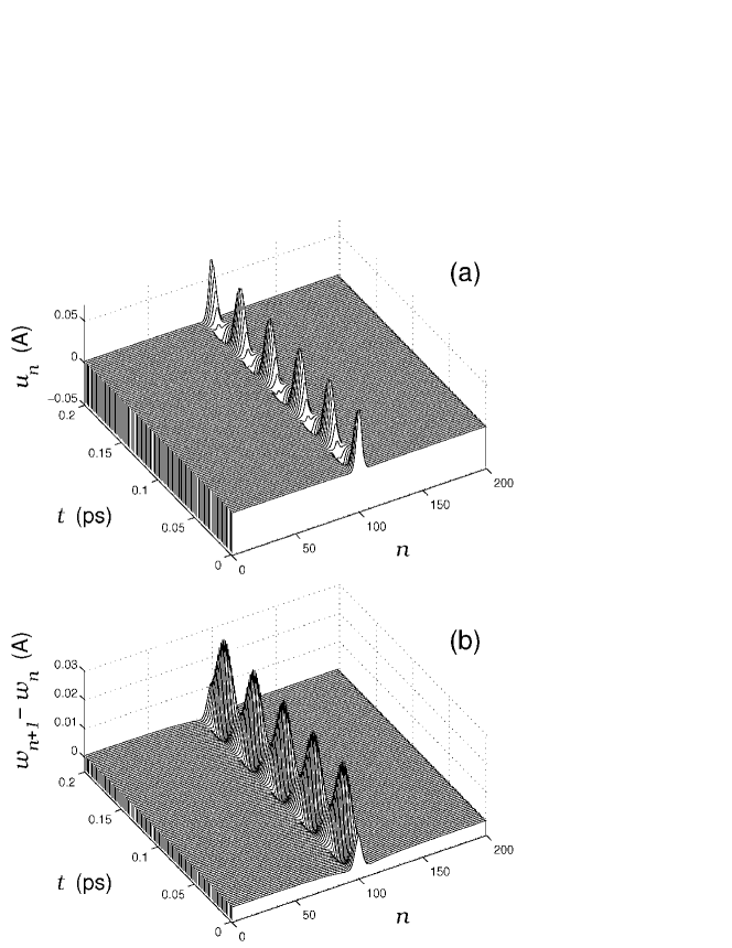
Figure 6: Periodic change of transversal $u_{n}$ and relative longitudinal displacements of zigzag $w_{n+1}-w_{n}$ in the localization region of optic breathers under parameters (56), $N=200$. Frequency of the breather $\omega=820.5$ cm^-1 is slightly lower than gap frequency.

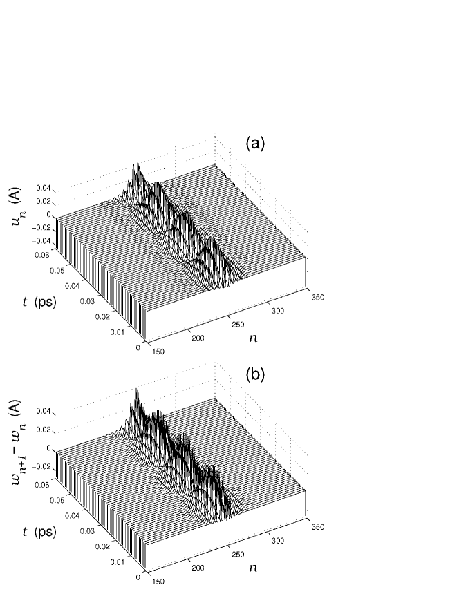
Figure 7: Periodic change of transversal $u_{n}$ and relative longitudinal displacements of zigzag chain $w_{n+1}-w_{n}$ in the localization region of optic breathers under parameter (57), $N=500$. Frequency of breather $\omega=928.4$ cm^-1 is slightly lower than frequency corresponding to low boundary of gap.

To consider an interaction of breathers with thermal vibrations of the chain, $N_{0}$ segments of the chain were inserted from every side into thermal bath with temperature T. Then the Langevin equations of motion

$$m{\displaystyle{{{\partial^{2}}\over{\partial t^{2}}}}}{u}_{n} = -\frac{\partial H}{\partial u_{n}}+\xi_{n}-\Gamma_{n}m\dot{u}_{n},$$

$$m{\displaystyle{{{\partial^{2}}\over{\partial t^{2}}}}}{v}_{n} = -\frac{\partial H}{\partial v_{n}}+\eta_{n}-\Gamma_{n}m\dot{u}_{n},$$ (58)

$$m{\displaystyle{{{\partial^{2}}\over{\partial t^{2}}}}}{w}_{n} = -\frac{\partial H}{\partial w_{n}}+\zeta_{n}-\Gamma_{n}m\dot{u}_{n},$$

where the Hamiltonian of the system H is given by Eq. (3), $\xi_{n}$, $\eta_{n}$, and $\zeta_{n}$ are random normally distributed forces describing the interaction of $n$th molecule with a thermal bath, coefficient of friction $\Gamma_{n}=0$, forces $\xi_{n}$, $\eta_{n}$, $\zeta_{n}=0$ for $N_{0}<n\leq N-N_{0}$ and $\Gamma_{n}=\Gamma$ for $n\leq N_{0}$ and $N-N_{0}<n\leq N$. Coefficient of friction $\Gamma=1/t_{r}$ , where $t_{r}$ is the relaxation of the velocity of the molecule. The random forces $\xi_{n}$, $\eta_{n}$, and $\zeta_{n}$ have correlation functions

$$\langle\xi_{n}(t_{1})\xi_{l}(t_{2})\rangle=\langle\eta_{n}(t_{1})\eta_{l}(t_{2})\rangle=\langle\zeta_{n}(t_{1})\zeta_{l}(t_{2})\rangle$$

$$=2m\Gamma k_{B}T\delta_{nl}\delta(t_{1}-t_{2}),$$

$$\langle\xi_{n}(t_{1})\eta_{l}(t_{2})\rangle=\langle\xi_{n}(t_{1})\zeta_{l}(t_{2})\rangle=\langle\eta_{n}(t_{1})\zeta_{l}(t_{2})\rangle=0,$$

$$1\leq n,l\leq N_{0},~{}~{}~{}N-N_{0}<n,l\leq N,$$

where $k_{B}$ is Boltzmann’s constant and $T$ is the temperature of heat bath.

The system (58) was integrated numerically by the standard forth-order Runge-Kutta method with a constant step of integration $\Delta t$. Numerically, the $\delta$-function was represented as $\delta(t)=0$ for $|t|>\Delta t/2$ and $\delta(t)=1/\Delta t$ for $|t|\leq\Delta t/2$, i.e. the step of numerical integration corresponded to the correlation time of the random force. In order to use the Langevin equation, it is necessary that $\Delta t\ll t_{r}$. Therefore, we chose $\Delta t=0.001$ ps and relaxation time $t_{r}=0.1$ ps.

To avoid an effect of friction coefficient on the behavior of breather, it was isolated from heat bath. For this, the stationary breather was situated at the center of the chain with $N_{0}=50$. In such a case, the breather can interact only with thermal phonons arising at the ends of the chain, which are connected with heat bath. The numerical integration of the equations (58) has shown that, contrary to isolated chain, the breathers in thermalized chain have a finite time of life. However, this time is large enough to provide a significant role of the breathers in different physical processes. Breaking of the breathers in thermalized chain is shown at Fig. 8 and 15 (a).

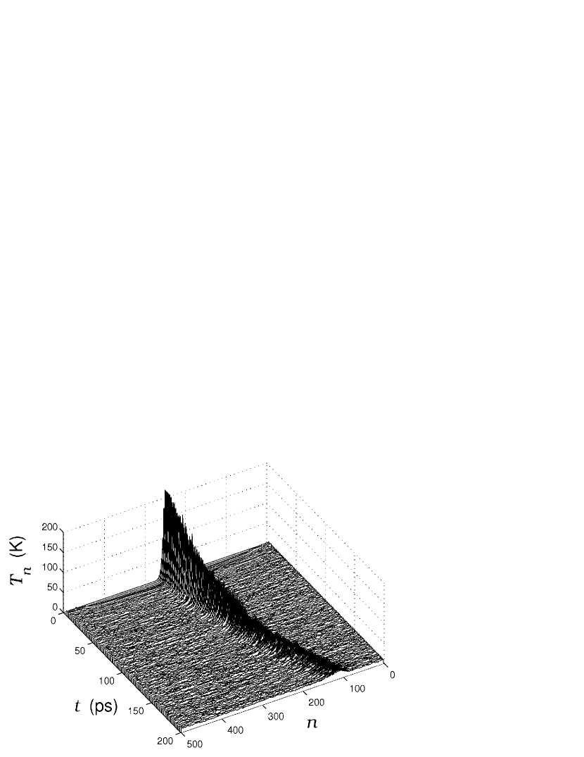
Figure 8: Breaking of the breather (frequency $\omega=928.4$ cm^-1) in thermalized chain ($N=500$, $T=10$ K, $\Lambda=529$ kJ/mol). Temporal dependence of current local magnitudes of temperature (kinetic energy of chain segments) $T_{n}$ is presented.

To estimate the breather time of life in thermalized chain let consider the temporal dependence of the energy (Fig. 9 and 13). It is seen, that the energy decreases monotonously by exponential low $E(t)=E(0)\exp(-\alpha t)$. One can determine the breather time of life as half of breaking period $t_{\alpha}=\ln 2/\alpha$b $(E(t_{\alpha})=E(0)/2)$. Dependence of $t_{\alpha}$ on the chain temperature $T$ is presented in table 5. We conclude, that breather time of life is proportional to ratio of its energy to temperature.

Table 5: Dependence of breathers time of life $t_{\alpha}$ on the chain temperature $T$ (frequency $\omega=820.5$ cm^-1, parameter $\Lambda=130.122$ kJ/mol and $\omega=928.4$ cm^-1, $\Lambda=529$ kJ/mol).

$\Lambda$ (kJ/mol)	$T$ (K)	1	2	3	5	10	20
130.122	$t_{\alpha}$ (ps)	180	94	68	46	33	22
529	$t_{\alpha}$ (ps)	1052	625	386	228	121	68

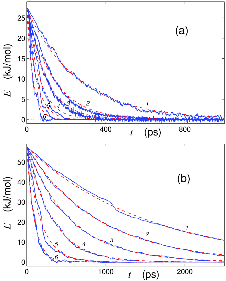
Figure 9: Decreasing the breather energy $E$ in thermalized chain with $\Lambda=130.1$ kJ/mol, $\omega=820.5$ cm^-1 (a) and $\Lambda=529$ kJ/mol, $\omega=928$ cm^-1 (b) under temperature $T=1$, 2, 3, 5, 10, 20 K (curves 1, 2,…,6). Solid lines determine temporal dependencies of breather energy for concrete realization of chain thermalization, dotted lines – corresponding exponential law $E(t)=E(0)\exp(-\alpha t)$.

Besides the considered breathers, the supersonic acoustic solitons can exist in PE chain [17]. Therefore, it is desirable to study their interaction with optic breathers [we choose further for definiteness the system of parameters (56)]. In such a case the acoustic solitons are caused by a local longitudinal compression of the chain (the properties of acoustic soliton were presented in [17]).

The collision of acoustic soliton with the stationary breather is shown at Fig. 10 (a). It is seen, that considered interaction does not lead to noticeable change of soliton energy, but the breather acquires a small momentum in the direction of the soliton motion. E.g., after collision of the soliton with velocity $s=1.024s_{0}$, where $s_{0}=7790$ m/s – velocity of long wavelength optic phonons, the breather with frequency $\omega=820.5$ cm^-1 becomes to move with constant velocity $s=0.0255s_{0}$. After every new collision, the breather velocity increases attaining the value $s=0.106s_{0}$ in limit.

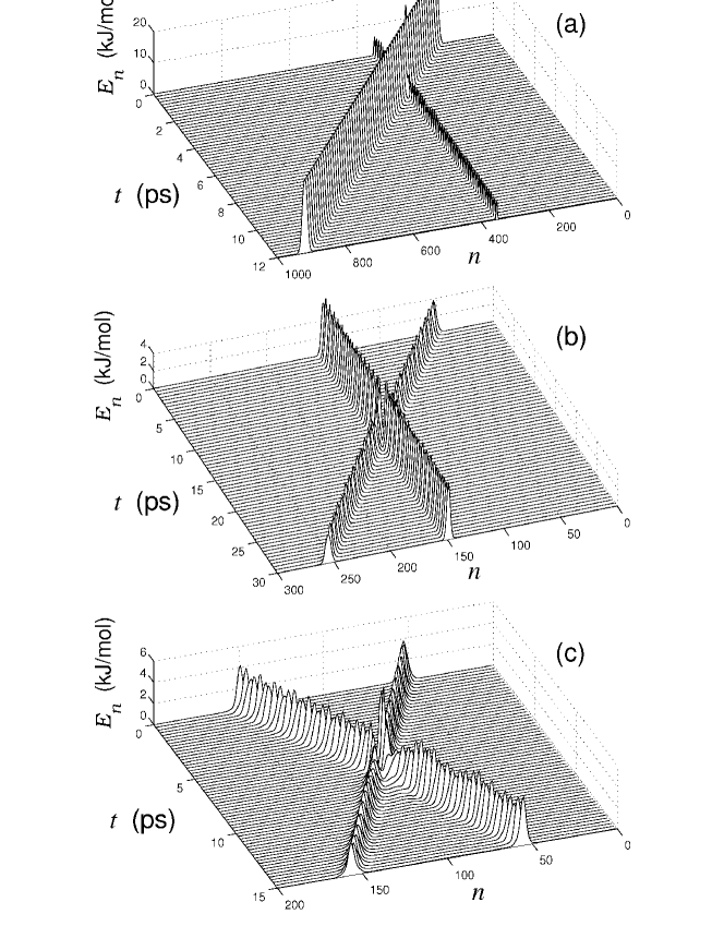
Figure 10: Collision of supersonic acoustic soliton with stationary optic breather ($\omega=820.5$ cm${}^{-}1$) (a), collision of moving breather (velocity $s=0.106s_{0}$) with stationary one (b) and elastic collision of two moving breathers (c). The temporal dependence of energy distribution $E_{n}$ along the chain is shown.

The motion of the breather is accompanied by phonon irradiation with low intensity that leads to decreasing of breather energy. The temporal dependence of the breather energy is shown at 11. It is well seen that change of velocity and energy decreasing may be fixed at very large time only ($\sim 10$ ns).

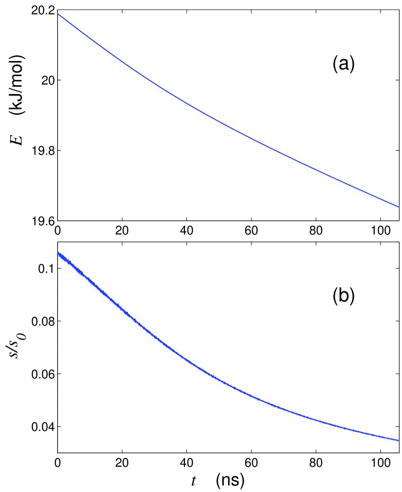
Figure 11: Decreasing the breather energy $E$ (a) and dimensionless breather velocity $s/s_{0}$ (b) in PE chain.

It is necessary to note that propagating breather has the frequency slightly exceeding the low boundary of frequency spectrum. So, we deal here with the breathers in the propagation zone of optic spectrum. However, the time of life in this case turns out also to be large enough as well as in the case of breather in the gap between acoustic and optic branches of the dispersion curve. Actually, let us consider the collision of propagating breather ($\omega=830$ cm^-1) with stationary one ($\omega=820$ cm^-1) [see Fig. 10 (b)] and collision of two propagating breathers ($\omega=830$ cm^-1) [see Fig. 10 (c)]. One can see that the breathers with frequency in propagation zone can move freely without any noticeable changes and interact with similar or stationary ones as elastic particles – they exchange by momentum without any energy decreasing.

In thermalized chain both propagating and stationary breathers have the time of life, which is proportional to ratio of breathers energy to temperature and does not noticeably depend on the breather velocity (Fig. 12).

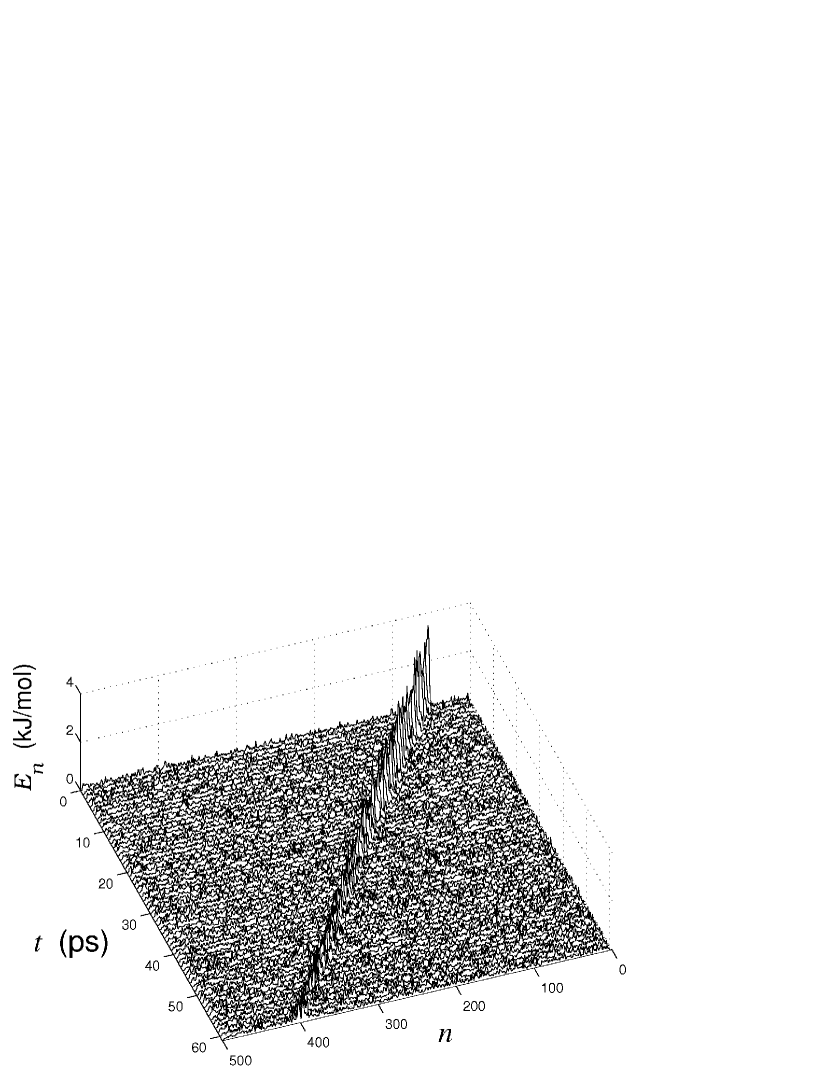
Figure 12: Breaking of moving breather (velocity $s=0.106s_{0}$) in thermalized chain (temperature $T=5$K). Temporal dependence of energy distribution along the chain $E_{n}$ is shown.

We have shown that the optic breathers can exist in both isolated chain and chain interacting with neighbor ones in the crystals. As this takes place the characteristics of the breather are not depend noticeably on the intermolecular interactions. In this case we can use approximation of immovable neighbor chains. Corresponding Hamiltonian (3) has a view

$$H = \sum_{n=-\infty}^{+\infty}\{\frac{1}{2}m[\dot{u}_{n}^{2}+\dot{v}_{n}^{2}+\dot{w}_{n}^{2}]$$

$$+[p_{1}+p_{2}\cos(\phi_{n})+p_{3}\cos(3\phi_{n})]$$

$$+\frac{1}{2}\Lambda[\cos(\theta_{n})-\cos(\theta_{0})]^{2}$$

$$+{\cal D}[1-e^{-q(\rho_{n}-\rho_{0})}]^{2}+W(u_{n},v_{n},w_{n})\},$$

where the function $W(u_{n},v_{n},w_{n})$ describes the interchain interaction. Detail description of this approach is given in [21].

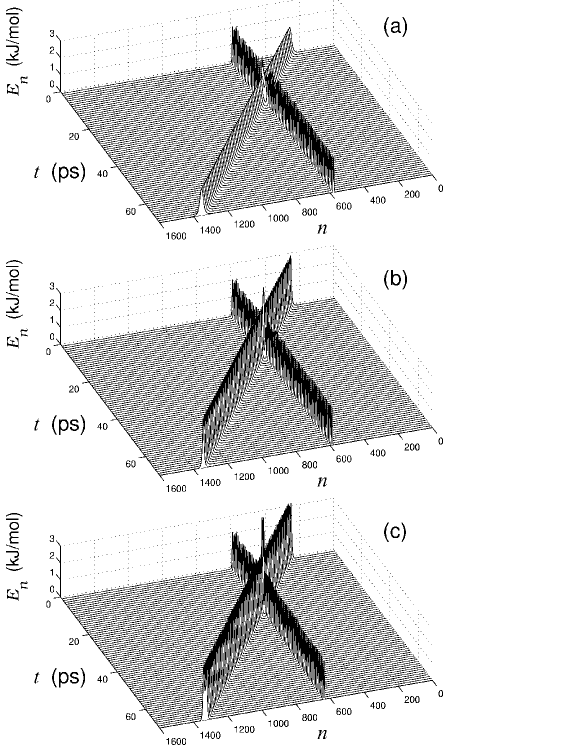
Figure 13: Passage of topological solitons (velocity $s=0.25s_{0}$) with charge ${\rm\bf q}=(1,0)$ (a), ${\rm\bf q}=(0.5,0.5)$ (b), and ${\rm\bf q}=(0,1)$ (c) through static breather (frequency $\omega=820.5$ cm^-1).

Figure 14: Breaking of the stationary breather (frequency $\omega=820.5$ cm^-1) as a result of collision with topological solitons with integer charge ${\rm\bf q}=(-1,0)$ (a) and half-integer charge ${\rm\bf q}=(-0.5,0.5)$ (b) (velocity of topological soliton $s=0.25s_{0}$).

Figure 15: Breaking of the stationary (a) and bound state (b) of the stationary breather with topological soliton [charge ${\rm\bf q}=(1,0)$] in thermalized chain with T=10K.

If taking into account interchain interaction, three types of topological solitons with topological charges ${\bf q}=(q_{1},q_{2})$ appear. Their properties are described in [21]. The solutions of the first type have topological charge q$=(\pm 1,0)$ and describe a localized longitudinal extension (compression) of the chain by one period. The solutions of the second type have the charge q$=(\pm 0.5,0.5)$ and describe a longitudinal extension (compression) of the chain by halved period and simulations twist by $180^{\circ}$. The solutions of the third type have the charge q$=(0,1)$ and describe the twist of the chain by $360^{\circ}$. All these topological solutions have subsonic spectra of velocities and can move without phonon irradiation.

We considered an interaction of stationary optic breather having frequency $\omega=820.5$ cm^-1 with moving topological solitons. As it is seen from Fig. 13 such an interaction is elastic one if first component of topological charge $q_{1}\leq 0$, i.e. if a compression in the localization region is absent. In opposite case, when $q_{1}<0$, the interaction with topological soliton leads to breaking the breather – see Fig. 14. Moreover, the bound state of breather and topological soliton ($q_{1}>0$) may be energetically profitable. Such a coupling increases the lifetime of breather in thermalized chain [compare Fig. 15 (a) and (b)].

10 Conclusion

The optic breathers which are localized coupled longitudinal-transversal nonlinear excitations can exist in both attenuation and propagation zones of PE crystal. In spite approximate analytical solution for breathers has been obtained using a model of isolated chain, we confirmed numerically not only validity of such a model but revealed also that the parameters of breathers change unnoticeably if taking into account interchain interaction. The reason is a weakness of interchain interaction in comparison to intrachain one. Such a weakness is especially clear for optic excitations. The breathers demonstrated stability to mutual collision and have large enough time of life in the presence of thermal excitations. The interaction of optic breathers with supersonic and subsonic (topological) solitons may be both elastic and inelastic dependent on their parameters.

The authors (L. I. M. and A. V. S.) thank the Region Rhone-Alpes and the Russian Foundation of Basic Research (awards 04-02-17306 and 04-03-32119), respectively for financial support.

References

• [1] J. Kirkwood, The Skeletal Modes of Vibration of Long Chain Molecules, J. Chem. Phys. 7, 506 (1939).
• [2] M. Magno and R. Lutz, Discrete buckling model for corrugated beam, European J. of Mechanics A/Solids 21, 661 (2002).
• [3] J. Skinner and P. Wolynes, Transition state and Brownian motion theories of solitons, J. Chem. Phys. 73, 4015 (1980).
• [4] R. Boyd, Relaxation processes in crystalline polymers: experimental behaviour - a review, Polymer 26, 323 (1985).
• [5] E. Zubova, N. Balabaev, and L. Manevitch, Diffusion of topological solitons and dielectric $\alpha_{c}$ relaxation in a polymeric crystal, J. Exp. Theor. Phys., 94, 759 (2002)
• [6] V. V. Ginzburg and L. I. Manevitch, On the theory of melting polymer crystals, Colloid and Polymer Science 269, 867 (1991).
• [7] O. V. Gendelman and L. I. Manevitch, Nonlinear dynamics of the diatomic Toda lattice and the problem of thermal conductivity of quasi-one-dimensional crystals, Soviet Phys. JETP 75, 271 (1992).
• [8] O. V. Gendelman and A. V. Savin, Normal Heat Conductivity of the One-Dimensional Lattice with Periodic Potential of Nearest-Neighbor Interaction Phys. Rev. Lett. 84, 2381 (2000).
• [9] H. Dvey-Aharon, P. Taylor, and A. Hopfinger, Dynamics of the Field-Induced Phase Transition to the Polar Alpha-Phase in Poly(vinylidene Fluoride), J. Appl. Phys, 51, 5184 (1980).
• [10] L. I. Manevitch, Solitons in Polymer Physics, Polymer Science C 4, 117 (2001).
• [11] L. I. Manevitch, L. Zarkhin, N. Enikolopyan, Nonlinear dynamics and the problem of polymer fracture, J. Appl. Polym. Science 39, 2245 (1990)
• [12] V. V. Ginzburg and L. Manevitch, On the theory of dislocation in polymer crystals, Polymer Science A 34, 91 (1992).
• [13] V. V. Ginzburg and L. Manevitch, Dislocation dipoles in polymer crystals, Polymer Science A 34, 98 (1992).
• [14] A. I. Musienko, N. K. Balabaev, L. I. Manevitch, Modeling of dynamics of screw dislocations in a crystalline polyethylene, Doklady Akademii Nauk 384, 213 (2002) [Doklady Physical Chemistry 384, 101 (2002)].
• [15] A. I. Musienko, N. K. Balabaev, L. I. Manevitch, Modeling of dynamics of edge dislocations in a crystalline polyethylene Doklady Akademii Nauk 372, 782 (2000) [Doklady Physical Chemistry 372, 92 (2000)].
• [16] L. I. Yakushevich, A. V. Savin, and L. I. Manevitch, Nonlinear dynamics of topological solitons in DNA. Phys. Rev. E 66, 016614 (2002).
• [17] L. I. Manevitch and A. V. Savin, Solitons in crystalline polyethylene: Isolated chains in the transconformation. Phys. Rev. E 55, 4713 (1997).
• [18] N. K. Balabaev, O. V. Gendelman, L. I. Manevitch, Supersonic motion of vacancies in a polyethylene crystal. Phys. Rev. E 64, 036702 (2001).
• [19] B. Sumpter, D. Noid, G. Liang, and B. Wunderlich, Adv. Polym. Sci. 116, 27 (1994).
• [20] F. Zhang, Molecular-dynamics simulation of solitary waves in polyethylene. Phys. Rev. E 56, 6077 (1997).
• [21] A. V. Savin, L. I. Manevitch, Solitons in crystalline polyethylene: A chain surrounded by immovable neighbors. Phys. Rev. B 58, 11386 (1998).
• [22] E. A. Zubova, N. K. Balabaev, L. I. Manevitch, A. Tsyqurov, Dynamics of point-like defects of torsion and tension in polymer crystal, JETP 91, 515 (2000).
• [23] G. Kopidakis and S. Aubry, Discrete breathers in realistic models:hydrocarbon structures. Physica B 296, 237 (2001).
• [24] A. V. Savin and L. I. Manevitch, Discrete breathers in a polyethylene chain. Phys.Rev. B 67, 144302 (2003).
• [25] S. Aubry, Breathers in nonlinear lattices: Existence, linear stability and quantization. Physica D 103, 201 (1997).
• [26] A. V. Savin and O. V. Gendelman, Heat conduction in one-dimensional lattices with on-site potential. Phys. Rev. E 67, 041205 (2003).
• [27] D.K. Campbell, S. Flach and Yuri S. Kivshar, Physics Today, 1, 43, (2004).