Bivariate $t$-distribution for transition matrix elements in Breit-Wigner to Gaussian domains of interacting particle systems

Abstract

Interacting many-particle systems with a mean-field one body part plus a chaos generating random two-body interaction having strength $\lambda$, exhibit Poisson to GOE and Breit-Wigner (BW) to Gaussian transitions in level fluctuations and strength functions with transition points marked by $\lambda=\lambda_{c}$ and $\lambda=\lambda_{F}$, respectively; $\lambda_{F}>>\lambda_{c}$. For these systems theory for matrix elements of one-body transition operators is available, as valid in the Gaussian domain, with $\lambda>\lambda_{F}$, in terms of orbitals occupation numbers, level densities and an integral involving a bivariate Gaussian in the initial and final energies. Here we show that, using bivariate $t$-distribution, the theory extends below from the Gaussian regime to the BW regime up to $\lambda=\lambda_{c}$. This is well tested in numerical calculations for six spinless fermions in twelve single particle states.

Two-body random matrix ensembles apply in a generic way to finite interacting many fermion systems such as nuclei Br-81 ; Ko-01 , atoms Fl-94 ; An-03 , quantum dots Al-01 , small metallic grains Pa-02 etc. A common feature of all these systems is that their hamiltonian ($H$) consists of a mean-field one-body [$h(1)]$ plus a complexity generating two-body [$V(2)$] interaction. With this, one has EGOE(1+2), the embedded Gaussian orthogonal ensemble of one plus two-body interactions operating in many particle spaces Ko-01 ; for more complete definition of EGOE(1+2) for $m$ fermions in $N$ single particle states see EGOE . Most significant aspect of EGOE(1+2) is that as $\lambda$, the strength of the random (represented by GOE) two-body interaction [in $H=h(1)+\lambda V(2)$], changes, in terms of state density, level fluctuations, strength functions and entropy DEN , the ensemble admits three chaos markers. Firstly, it is well known that the state densities take Gaussian form, for large enough $m$, for all $\lambda$ values Mo-75 . With $\lambda$ increasing, there is a chaos marker $\lambda_{c}$ such that for $\lambda\geq\lambda_{c}$ the level fluctuations follow GOE, i.e. $\lambda_{c}$ marks the transition in the nearest neighbor spacing distribution from Poisson to Wigner form Ja-97 . As $\lambda$ increases further from $\lambda_{c}$, the strength functions (for $h(1)$ basis states) change from Breit-Wigner (BW) to Gaussian form and the transition point is denoted by $\lambda_{F}$ Fl-97 . The $\lambda_{c}\leq\lambda\leq\lambda_{F}$ region is called BW domain and the $\lambda>\lambda_{F}$ region is called Gaussian domain. As we increase $\lambda$ much beyond $\lambda_{F}$, there is a chaos marker $\lambda_{t}$ around which different definitions of entropy, temperature etc. will coincide and also strength functions in $h(1)$ and $V(2)$ basis will coincide. Thus $\lambda\sim\lambda_{t}$ region is called the thermodynamic region Ks-02 ; Ko-03 .

With the three chaos markers $\lambda_{c}$, $\lambda_{F}$ and $\lambda_{t}$, EGOE generates statistical spectroscopy, i.e. smoothed forms for state densities, orbit occupancies, strength sums [for example Gamow-Teller (GT) sums in nuclei, electric dipole ($E1$) sums in atoms], transition strengths themselves [for example: electric quadrupole($E2$), magnetic dipole ($M1$) and GT strengths in nuclei, $E1$ strengths in atoms and molecules etc.], information entropy in wavefunctions and transition strengths etc. The EGOE Gaussian state densities are being used to generate a theory (valid for $\lambda>\lambda_{c}$) for level densities with interactions Ho-03 . Similarly, theory for orbit occupancies and strength sums, as valid in BW to Gaussian regimes (i.e. for $\lambda>\lambda_{c}$) has been developed Ko-03 . However, for transition strengths (experimentally they are most important for probing wavefunctions structure of a quantum system), a theory valid only in the Gaussian domain is available Fr-88 ; To-86 ; Ks-00 . Although a theory was given by Flambaum et al for BW domain Fl-94 ; Fl-96 ; Fl-98 , it is well known to underestimate the exact values by a factor of 2 Fl-96 ; Ks-00 . Thus, a major gap (see the discussion in Ks-00 ) in understanding transition strengths is in extending the theory that works in the Gaussian domain, well into the BW domain. The purpose of this paper is to show that the bivariate $t$-distribution known in statistics will bridge this gap. As in Refs. Fl-98 ; Ks-00 , we restrict ourselves to one-body transition operators.

Given a Hamiltonian $H$ and its $m$-particle eigenstates $\left|E\right\rangle$, the transition strengths generated by a one-body transition operator $\cal{O}$ are denoted by $\left|\left\langle E_{f}\mid{\cal{O}}\mid E_{i}\right\rangle\right|^{2}$; ${\cal O}=\sum_{\alpha,\beta}\;\epsilon_{\alpha\beta}a^{\dagger}_{\alpha}a_{\beta}$ where $a^{\dagger}_{\alpha}$ creates a particle in the single particle state $\alpha$ and $a_{\beta}$ destroys a particle in the state $\beta$. Now the bivariate strength densities are defined by

$$I^{H,m}_{biv;{\cal O}}(E_{i},E_{f})=\left\langle\left\langle{\cal O}^{\dagger}\delta(H-E_{f}){\cal O}\delta(H-E_{i})\right\rangle\right\rangle^{m}=\left\langle\left\langle{\cal O}^{\dagger}{\cal O}\right\rangle\right\rangle^{m}\;\rho^{H;m}_{biv;{\cal O}}(E_{i},E_{f})\;.$$ (1)

In Eq. (1), $\left\langle\left\langle\;\;\right\rangle\right\rangle$ denotes trace. Note that $I_{biv;{\cal O}}$ is square of the matrix elements of ${\cal O}$ in $H$ eigenstates weighted by the state densities at the initial and final energies and the corresponding $\rho_{biv;{\cal O}}$ is normalized to unity. Moreover, one-body transition operators ${\cal O}$ will not change $m$. The bivariate moments of $\rho_{biv;{\cal O}}$ are defined by $M_{pq}=\left\langle\left\langle{\cal O}^{\dagger}H^{q}{\cal O}H^{p}\right\rangle\right\rangle^{m}/\left\langle\left\langle{\cal O}^{\dagger}{\cal O}\right\rangle\right\rangle^{m}$. With $M_{10}=\epsilon_{i}$ and $M_{01}=\epsilon_{f}$ defining the centroids of its two marginals, the bivariate central moments of $\rho_{biv;{\cal O}}$ are given by

$$\mu_{pq}=\left\langle\left\langle{\cal O}^{\dagger}\;\left(H-\epsilon_{f}\right)^{q}\;{\cal O}\;\left(H-\epsilon_{i}\right)^{p}\right\rangle\right\rangle^{m}\;/\;\left\langle\left\langle{\cal O}^{\dagger}{\cal O}\right\rangle\right\rangle^{m}\;\;.$$ (2)

Most important of these are $\mu_{20}=\sigma_{i}^{2}$ and $\mu_{02}=\sigma_{f}^{2}$, the variances of the two marginals and $\zeta=\mu_{11}/\sigma_{i}\sigma_{f}$, the bivariate correlation coefficient.

For EGOE(1+2), going well into the Gaussian domain [then EGOE(1+2) will be effectively EGOE(2)], it is well established that the bivariate strength densities take bivariate Gaussian form (this applies to nuclei Fr-88 ; To-86 ),

$$\begin{array}[]{l}\rho_{biv;{\cal O}}(E_{i},E_{f})\stackrel{{\scriptstyle\lambda>>\lambda_{F}}}{{\longrightarrow}}\rho_{biv-{\cal G};{\cal O}}(E_{i},E_{f};\epsilon_{i},\epsilon_{f},\sigma_{i},\sigma_{f},\zeta)=\displaystyle\frac{1}{2\pi\sigma_{i}\sigma_{f}\sqrt{(1-\zeta^{2})}}\;\;\times\\ \exp-\displaystyle\frac{1}{2(1-\zeta^{2})}\left\{\left(\frac{E_{i}-\epsilon_{i}}{\sigma_{i}}\right)^{2}-2\zeta\left(\frac{E_{i}-\epsilon_{i}}{\sigma_{i}}\right)\left(\frac{E_{f}-\epsilon_{f}}{\sigma_{f}}\right)+\left(\frac{E_{f}-\epsilon_{f}}{\sigma_{f}}\right)^{2}\;\;\right\}\;.\end{array}$$ (3)

An immediate question is how to extend this result well into the BW domain and up to $\lambda_{c}$ (note that GOE fluctuations operate for $\lambda>\lambda_{c}$ and hence in this regime it is possible to consider smoothed transition strengths). In a recent work, Angom et al An-04 showed that strength functions covering the BW to Gaussian regimes can be well represented by Student’s $t$-distribution. Following this result, here we conjecture that the bivariate strength density $\rho_{biv;{\cal O}}$ in Eq. (1) can be represented by the bivariate $t$-distribution,

$$\begin{array}[]{l}\rho_{biv-t;{\cal O}}(E_{i},E_{f};\epsilon_{i},\epsilon_{f},\sigma_{1},\sigma_{2},\zeta;\nu)=\frac{1}{2\pi\sigma_{1}\sigma_{2}\sqrt{1-\zeta^{2}}}\;\;\times\\ \left[1+\frac{1}{\nu(1-\zeta^{2})}\left\{\left(\frac{E_{i}-\epsilon_{i}}{\sigma_{1}}\right)^{2}-2\zeta\left(\frac{E_{i}-\epsilon_{i}}{\sigma_{1}}\right)\left(\frac{E_{f}-\epsilon_{f}}{\sigma_{2}}\right)+\left(\frac{E_{f}-\epsilon_{f}}{\sigma_{2}}\right)^{2}\right\}\right]^{-\frac{\nu+2}{2}}\;\;,\;\nu\geq 1\;.\end{array}$$ (4)

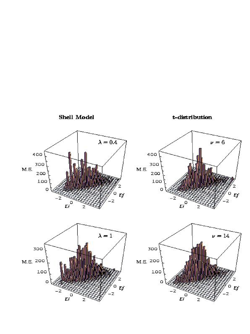
Figure 1: $E2$ transition strengths vs ($Ei$, $Ef$). The $E2$ transitions considered are $(0^{+},0)$ to $(2^{+},0)$; with $J$, $T$ and $\pi$ denoting angular momentum, isospin and parity, nuclear levels are denoted by $(J^{\pi},T)$. Calculations are for 6 valence nucleons in $(2s1d)$ shell and the hamiltonian matrix dimensions for these are 71 and 307 respectively. The hamiltonian employed is $H(\lambda)=h(1)+\lambda V(2)$ with the single particle energies defining $h(1)$ and two particle matrix elements defining $V(2)$ taken from Bw-88 and references therein (they define the so called Wildenthal’s W-interaction). The proton and neutron effective charges for the $E2$ operator are $e_{p}=1.29$ and $e_{n}=0.49$ respectively. All the calculations are carried out using the OXBASH computer code for Windows PC (2005-05 version) Ox-99 . In the figures the energies $Ei$ and $Ef$ are the energies of $(0^{+},0)$ and $(2^{+},0)$ levels respectively and they are zero centered and scaled to unit width. Similarly M.E. stands for $E2$ transition strengths and they are in units of $e^{2}fm^{4}$. The vertical bars in the figures give the total strength in a given bin area; in constructing the histograms bin size of 0.3 is taken for both $Ei$ and $Ef$. Although Eq. (4) is for EGOE(1+2), which is for spinless fermion systems, it can be applied directly to the shell model with good $(J^{\pi},T)$ states as described in Go-04 .

Properties of $\rho_{biv-t}$ are given in Jo-72 ; Hu-90 . Most important is that for $(\nu=1,\zeta=0)$, $\rho_{biv-t}$ gives bivariate BW (called bivariate Cauchy in statistics) distribution and as $\nu\rightarrow\infty$, $\rho_{biv-t}$ becomes bivariate Gaussian. Thus it has the correct limiting forms and the intermediate shapes are largely determined by the $\nu$ parameter. The marginal distributions of $\rho_{biv-t}$ are easily seen to be univariate $t$-distributions. In Eq. (4), in general $\epsilon_{i}$ and $\epsilon_{f}$ are the centroids of the two marginals of $\rho_{biv-t}$, however $\sigma_{1}$ and $\sigma_{2}$ will approach the marginal widths $\sigma_{i}$ and $\sigma_{f}$ only in the limit $\nu\rightarrow\infty$, i.e. for the bivariate Gaussian given in Eq. (3). In-fact, the second central moments $\mu_{20}=\sigma_{i}^{2}$ and $\mu_{02}=\sigma_{f}^{2}$ are related to $\sigma^{2}_{1}$ and $\sigma^{2}_{2}$ by $\mu_{20}=\frac{\nu}{\nu-2}\;\sigma_{1}^{2}$ and $\mu_{02}=\frac{\nu}{\nu-2}\;\sigma_{2}^{2}$ for $\nu>2$. However $\zeta$ remains to be the bivariate correlation coefficient. Exceptions to all these will occur for $\nu\leq 2$ and here (this happens only when $\lambda$ is very close to $\lambda_{c}$) one has to use quartiles (i.e. spreading widths) to define $\sigma_{1}$, $\sigma_{2}$ etc.; see Jo-72 ; Hu-90 for details. In order to test the applicability of the $t$-distribution, nuclear shell model calculations are performed for isoscalar $E2$ transitions in ²²Na nucleus. Fig. 1 shows the results for $\lambda=0.4$ and 1 in the shell model hamiltonian $H=h(1)+\lambda\,V(2)$; $\lambda=1$ gives realistic nuclear hamiltonian. The parameters $\sigma_{1}$ and $\sigma_{2}$ in Eq. (4) are determined via their relation to $\mu_{20}$ and $\mu_{02}$. The value of $\zeta=0.88$ is used as given by the exact $E2$ strengths. Clearly (ignoring the deviations near the ground states), the $t$-distribution gives a good description of the transition strengths with $\nu=6$ for $\lambda=0.4$ and with a large $\nu$ value, as expected, for $\lambda=1$.

In larger spectroscopic spaces, instead of using a single $t$-distribution, to represent transition strength densities, it is more appropriate to partition the space. Decomposing the space into subspaces defined by $h(1)$ eigenvalues ${\cal E}$, constructing the strength distribution generated by $h(1)$ alone, spreading this distribution by convolution with a $t$-distribution generated by $V(2)$ and then applying some simplifying assumptions, as described in detail in Ks-00 where this procedure is applied to bivariate Gaussian spreadings, it is seen that the transition strengths can be given by,

$$\left|\left\langle E_{f}\mid{\cal{O}}\mid E_{i}\right\rangle\right|^{2}=\sum_{\alpha,\beta}\;\left|\epsilon_{\alpha\beta}\right|^{2}\left\langle n_{\beta}(1-n_{\alpha})\right\rangle^{E_{i}}\overline{D(E_{f})}\;\;{\cal F}\;;$$ (5a)

$${\cal F}=\displaystyle\int^{+\infty}_{-\infty}\rho_{biv-t;{\cal{O}}}(E_{i},\;E_{f};\;{\cal{E}}_{i},\;{\cal{E}}_{f}={\cal{E}}_{i}-\epsilon_{\beta}+\epsilon_{\alpha},\;\sigma_{1},\;\sigma_{2},\;\zeta;\nu)\;d{\cal{E}}_{i}$$ (5b)

In Eq. (5a) $\overline{D}(E_{f})$ denotes mean-spacing at the energy $E_{f}$, $\epsilon_{\alpha\beta}$ are single particle matrix elements of ${\cal O}$ and $\left\langle n_{\beta}(1-n_{\alpha})\right\rangle^{E_{i}}\sim\left\langle n_{\beta}\right\rangle^{E_{i}}\,\left\langle(1-n_{\alpha})\right\rangle^{E_{i}}$ with $\left\langle n_{\alpha}\right\rangle^{E_{i}}$ giving occupation probability for the single particle state or orbital $\alpha$. Most remarkable is that the integral for ${\cal F}$ in Eq. (5b) can be carried out exactly for any $\nu$ and this gives,

$${\cal F}=\frac{\Gamma(\frac{\nu+1}{2})}{\sqrt{\pi}\Gamma(\frac{\nu}{2})}\;\;\frac{1}{\sqrt{\nu(\sigma_{1}^{2}+\sigma_{2}^{2}-2\zeta\sigma_{1}\sigma_{2})}}\;\;\left[1+\frac{\Delta^{2}}{\nu(\sigma_{1}^{2}+\sigma_{2}^{2}-2\zeta\sigma_{1}\sigma_{2})}\right]^{-\frac{\nu+1}{2}}\;;\;\;\Delta=E_{f}-E_{i}+\epsilon_{\beta}-\epsilon_{\alpha}$$ (6)

Note that, for $\nu>2$, $\sigma_{1}$ and $\sigma_{2}$ are related (as given above) to the marginal variances $\mu_{20}$ and $\mu_{02}$ of $\left|\left\langle E_{f}\mid{\cal{O}}\mid E_{i}\right\rangle\right|^{2}$. Also, the correlation coefficient $\zeta\sim\left\langle{\cal O}^{\dagger}V{\cal O}V\right\rangle/\left\langle{\cal O}^{\dagger}{\cal O}\right\rangle\left\langle VV\right\rangle$; see Fr-88 . More importantly, as $\nu\rightarrow\infty$, Eq. (6) goes exactly to Eq. (6) of Ks-00 as it should be.

To test the theory given by Eqs. (5a) and (6), numerical calculations are carried out for various $\lambda$ values using 25 member EGOE(1+2) ensemble $\{H\}=h(1)+\lambda\{V(2)\}$ in the 924 dimensional $N=12$, $m=6$ space; $h(1)$ is defined by the single particle energies $\epsilon_{i}=(i)+(1/i)$, $i=1,2,\ldots,12$ and the variance of $V(2)$ matrix elements in two-particle spaces is chosen to be unity. The one-body transition operator employed in the calculations is ${\cal O}=a^{\dagger}_{2}a_{9}$ as in Ks-00 . For the system considered, $\lambda_{c}\sim 0.06$, $\lambda_{F}\sim 0.2$ and $\lambda_{t}\sim 0.3$. Results for six different $\lambda$ values, going from BW to Gaussian domains, are shown in Fig. 2. Clearly Eqs. (5a) and (6) obtained via the $t$-distribution describe the exact EGOE(1+2) transition strengths as we go from the BW domain with $\lambda=0.08$ to the Gaussian domain with $\lambda=0.3$ with $\nu$ changing from 2.4 to 14; $\nu\sim 2-6$ for $\lambda_{c}<\lambda<\lambda_{F}$ and $\nu\sim 6-15$ for $\lambda_{F}<\lambda<\lambda_{t}$. The exact distributions give $\zeta\simeq 0.5$ but in the fits $\zeta$ is also varied (see Fig. 2) and this to some extent takes into account some of the approximations that led to the simple form given by Eqs. (5a) and (6). More importantly, the results in Fig. 2 confirm that we have a good method for the calculation of transition strengths in BW domain. A calculation is also performed for $\lambda=0.06$ by fixing $\sigma_{1}$ and $\sigma_{2}$ using the spreading widths of the marginals of the strength distribution and using $\zeta$ value same as that obtained for $\lambda=0.08$. Then the deduced $\nu$ value is $1.5$. This and the comparisons in Fig. 2 clearly emphasize the role of the bivariate correlation coefficient $\zeta$ in BW domain and without $\zeta$ it is not possible to get a meaningful description (it should be mentioned that the theory in the BW domain given before Fl-98 ; Ks-00 uses only the marginals of the $t$-distribution with $\nu=1$ and $\zeta=0$). Thus all the problems seen before Ks-00 ; Fl-96 in the BW domain are cured by the bivariate-$t$ distribution with the two parameters $(\nu,\,\zeta)$.

In conclusion, random matrix ensembles generated by a mean-field plus a random two-body interaction generate three chaos markers. They in-turn provide a basis for statistical spectroscopy. The theory for transition strengths is now extended (from Gaussian domain) to BW domain down up to the $\lambda_{c}$ marker by employing bivariate $t$-distribution. With atoms exhibiting a clear transition from BW to Gaussian domain (an example for CeI to SmI atoms was shown in An-04 ), it is expected that the theory given by Eqs. (5a) and (6) will be useful in the calculation of dipole transition strengths in the quantum chaotic domain of atoms.

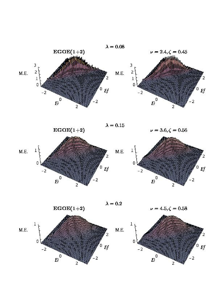
Figure 2: Transition strengths $\left|\left\langle E_{f}\mid{\cal O}\mid E_{i}\right\rangle\right|^{2}$ vs $(Ei,Ef)$ for $\lambda=0.08$, 0.15, 0.2, 0.25, 0.28 and 0.3. In the figures $Ei={\hat{E}}_{i}=(E_{i}-\epsilon)/\sigma$ and $Ef={\hat{E}}_{f}=(E_{f}-\epsilon)/\sigma$ where $\epsilon$ and $\sigma$ are the centroids and widths of the state densities. Similarly M.E. stands for the strengths $\left|\left\langle E_{f}\mid{\cal O}\mid E_{i}\right\rangle\right|^{2}$. The EGOE(1+2) system and the one-body transition operator ${\cal O}$ are defined in the text. In all the calculations the strengths in the window ${\hat{E}}_{i}\pm\frac{\Delta^{\prime}}{2}$ and ${\hat{E}}_{f}\pm\frac{\Delta^{\prime}}{2}$ are summed and plotted at (${\hat{E}}_{i}$, ${\hat{E}}_{f}$); $\Delta^{\prime}$ is chosen to be $0.1$. It should be noted that the total strength is 252. As $\lambda$ changes from 0.08 to 0.3, the $\nu$ value changes from 2.4 to 14 and the bivariate correlation coefficient $\zeta$ changes from 0.45 to 0.62. Note the change in the scales for M.E. in the figures.

FIG. 2 (Cont’d)

References

- (1) T.A. Brody, J. Flores, J.B. French, P.A. Mello, A. Pandey, and S.S.M. Wong, Rev. Mod. Phys. 53, 385 (1981).
- (2) V.K.B. Kota, Phys. Rep. 347, 223 (2001).
- (3) V.V. Flambaum, A.A. Gribakina, G.F. Gribakin, and M.G. Kozlov, Phys. Rev. A 50, 267 (1994); V.V. Flambaum, A.A. Gribakina, G.F. Gribakin, and I.V. Ponomarev, Physica D 131, 205 (1999).
- (4) D. Angom and V. K. B. Kota, Phys. Rev. A 67, 052508 (2003); 71, 042504 (2005).
- (5) Y. Alhassid, Ph. Jacquod, and A. Wobst, Phys. Rev. B 61, R13357 (2000); Physica E9, 393 (2001); Ph. Jacquod and A.D. Stone, Phys. Rev. Lett. 84, 3938 (2000); Phys. Rev. B 64, 214416 (2001); Y. Alhassid and A. Wobst, Phys. Rev. B 65, 041304 (2002).
- (6) T. Papenbrock, L. Kaplan, and G.F. Bertsch, Phys. Rev. B 65, 235120 (2002).
- (7) The EGOE(2) for () spin-less fermion systems with the particles distributed say in single particle states (, ) is generated by defining the Hamiltonian H, which is two-body, to be GOE in the 2-particle space and then propagating it to the -particle spaces by using the geometry (direct product structure) of the -particle spaces. Then EGOE(1+2) is defined by where denotes an ensemble. The mean-field one-body Hamiltonian is a fixed one-body operator defined by the single particle energies with average spacing (note that is the number operator for the single particle state ). The is EGOE(2) with unit variance for the two-body matrix elements and is the strength of the two-body interaction (in units of ). Thus, EGOE(1+2) is defined by the four parameters and without loss of generality we put .
- (8) state densities where denotes average. Given the mean-field basis states , the strength functions (one for each ) . Similarly the number of principle components NPC and the closely related information entropy .
- (9) K.K. Mon and J.B. French, Ann. Phys. (N.Y.) 95, 90 (1975); L. Benet, T. Rupp, and H.A. Weidenmüller, Ann. Phys. (N.Y.) 292, 67 (2001).
- (10) S. Aberg, Phys. Rev. Lett. 64, 3119 (1990); Ph. Jacquod and D.L. Shepelyansky, Phys. Rev. Lett. 79, 1837 (1997).
- (11) V.V. Flambaum and F.M. Izrailev, Phys. Rev. E 56, 5144 (1997); Phys. Rev. E 61, 2539 (2000); V.K.B. Kota and R. Sahu, Phys. Rev. E 64, 016219 (2001); preprint nucl-th/0006079; Ph. Jacquod and I. Varga, Phys. Rev. Lett. 89, 134101 (2002).
- (12) V.K.B. Kota and R. Sahu, Phys. Rev. E 66, 037103 (2002); M. Horoi, V. Zelevinsky, and B.A. Brown, Phys. Rev. Lett. 74, 5194 (1995).
- (13) V.K.B. Kota, Ann. Phys. (N.Y.) 306, 58 (2003).
- (14) J.B. French and V.K.B. Kota, Phys. Rev. Lett. 51, 2183 (1983); V.K.B. Kota and D. Majumdar, Nucl. Phys. A604, 129 (1996); M. Horoi, J. Kaiser, and V. Zelevinsky, Phys. Rev. C 67, 054309 (2003); M. Horoi, M. Ghita, and V. Zelevinsky, Phys. Rev. C 69, 041307(R) (2004).
- (15) J.B. French, V.K.B. Kota, A. Pandey, and S. Tomsovic, Phys. Rev. Lett. 58, 2400 (1987); Ann. Phys. (N.Y.) 181, 235 (1988).
- (16) S. Tomsovic, Ph. D. Thesis, University of Rochester (1986) (unpublished); V.K.B. Kota and D. Majumdar, Z. Phys. A 351, 365 (1995); 351, 377 (1995).
- (17) V.K.B. Kota and R. Sahu, Phys. Rev. E 62, 3568 (2000).
- (18) V.V. Flambaum, G.F. Gribakin, and F.M. Izrailev, Phys. Rev. E 53, 5729 (1996).
- (19) V.V. Flambaum, A.A. Gribakina, and G.F. Gribakin, Phys. Rev. A 58, 230 (1998).
- (20) D. Angom, S. Ghosh, and V.K.B. Kota, Phys. Rev. E 70, 016209 (2004).
- (21) N.L. Johnson and S. Kotz, Distributions in Statistics: Continuous Multivariate Distributions (John Wiley & Sons, Inc., New York, 1972).
- (22) T.P. Hutchinson and C.D. Lai, Continuous Bivariate Distributions, Emphasizing Applications (Rumsby Scientific publishing, Adelaide, 1990).
- (23) B.A. Brown and B.H. Wildenthal, Ann. Rev. Nucl. Part. Sci. 38, 29 (1988).
- (24) B.A. Brown, A. Etchegoyen, N.S. Godwin, W.D.M. Rae, W.A. Richter, W.E. Ormand, E.K. Warburton, J.S. Winfield, L. Zhao, and C.H. Zimmerman, MSU-NSCL report number 1289 (2005); B.A. Brown, private communication.
- (25) J.M.G. Gómez, K. Kar, V.K.B. Kota, R.A. Molina and J. Retamosa, Phys. Rev. C 69, 057302 (2004).