Variational method for locating invariant tori

Abstract

We formulate a variational fictitious-time flow which drives an initial guess torus to a torus invariant under given dynamics. The method is general and applies in principle to continuous time flows and discrete time maps in arbitrary dimension, and to both Hamiltonian and dissipative systems.

I Introduction

Analysis of dynamical systems in terms of invariant phase space structures provides important insights into the behavior of physical systems. The simplest such invariants are equilibria, points in phase space which are stationary solutions or 0-dimensional invariants of the flow. They and their stable/unstable manifolds yield information about the topology of the flow. The role that the next class of flow invariants, periodic orbits, play in the topological organization of phase space and the computation of long time chaotic dynamics averages is well known (for an overview, see Ref. Bchaos ). A periodic orbit is topologically a circle or an invariant 1-torus for a flow, and a set of discrete points or an invariant 0-torus for a map, embedded in a $d$-dimensional phase space. Higher dimensional invariant tori also frequently play an important role in the dynamics; we refer the reader to Ref. WysMeis05 for some of the references to this literature. Invariant tori of dimension lower than the dimension of the dynamical flow can be normally hyperbolic Treshev94 ; hir77inv . KAM theory implies that invariant tori occur in Cantor sets, and such tori play key roles in the phase-space transport mac84tr ; mac84st . For 2-degree of freedom Hamiltonian flows (i.e., 4-dimensional phase space), 2-dimensional invariant tori act as barriers to diffusion through phase space, and for higher dimensional flows such structures act as effective barriers (Arnold diffusion). In dissipative systems such as Newtonian fluids, quasi-periodic motion on two or higher dimensional tori is one of the routes to the eventual turbulent motion cvt89b ; nhouse78 .

There are many methods for determining periodic orbits available in the literature Bchaos ; chen87orb ; mes87new . The lack of comparably effective methods for the determination of higher dimensional invariant structures has stymied the exploration of the phase spaces of high-dimensional flows, a focus of much recent research WysMeis05 ; delaLlave04:348 .

Signal processing methods like frequency analysis laskar ; lask92 , based on the analysis of trajectories, can detect elliptic invariant tori since these tori influence significantly the behavior of nearby trajectories. Bailout methods cart02bail ; bab00dyn can effectively locate the elliptic regions in a non-integrable system, by embedding the dynamical system into a larger phase space. Ref. bot95find describes a variational technique designed to find regular orbits in a phase space with mixed dynamics. However, these methods can only detect trajectories with non-positive Lyapunov exponents. They single out regular motions in a phase space but can not exactly determine a torus unless it is stable. Due to their relative ease of identification, in particular cases periodic orbits are used to study invariant tori and their breakup. For example, in Greene’s criterion approach gree79 ; mack92 ; tom96num one studies a sequence of periodic orbits which converges to a given invariant torus. Such approaches have been mainly applied to the determination of tori of Hamiltonian systems with 2 degrees of freedom.

Other techniques to determine invariant tori are specific to the phase space dynamics of the system under consideration, most often a Hamiltonian system. Early attempts like spectral balance method were based on the computation of quasi-periodic orbits park89num ; Simo90 , the closure of which constitutes the invariant torus. To overcome the small divisor problems associated with the flow on a torus, recent research employed a geometric point of view and focused on the invariant torus itself. Efforts are devoted to find the solution of the so-called invariance condition which ensures the invariance of a parametrized object in phase space. Invariance conditions are functional equations for maps kev85num ; deb94num ; moo96com ; vel87new ; br97alg ; die91num and first-order partial differential equations (PDEs) for flows min97com ; ge98con ; sch05con . These equations can be solved by Newton’s method or Hadamard graph transform technique hir77inv . In view of the periodicity in the angle variables, Fourier transforms are widely used in the computation lop05rel ; war87inv ; CasJorb00 ; jor03inv ; sh05fou ; kaa95con ; war91clo . For Hamiltonian systems, the action principle and the Hamilton-Jacobi equation are also frequently used in the calculation of periodic and quasi-periodic orbits per74var ; per79var ; kook89 ; war87inv ; Mather91 ; gab92iter .

In this paper we introduce a method to solve the invariance condition equation and obtain invariant $m$-tori of flows and maps embedded in $d$-dimensional phase spaces. It has a variational structure which guarantees the global convergence. The method is a generalization of the variational “Newton descent” method originally developed to locate periodic orbits of flows CvitLanCrete02 ; lanVar1 , which can be viewed as a variant of multi-shooting method in boundary value problems kellbv ; bl ; nr . When the representative points on the guess torus achieve a near-continuous distribution, a PDE is derived which governs their evolution to a true invariant torus. In spirit, this is similar to the approach used in Ref. war87inv and thus high accuracy is expected. However, our method is stable and thus applies to more general cases, including the searches for partially hyperbolic tori embedded in the chaotic regions of phase space. In a general dynamical system, the phase space structure can be extremely complex, and the global stability of our algorithm is of key importance for the the efficiency of our searching program. In our numerical computation, an adaptive scheme is used which keeps changing the step size according to the smoothness of the evolution. In addition to the adaptive step size, we further speed up our searches by utilizing the continuity of the variational evolution equations. These points will be explained in detail in what follows.

In Sec. II we derive the variational equation which governs the fictitious time dynamics. The numerical implemention of this equation is discussed in Sec. III. The method is further illustrated in Sec. IV through its application to the determination of 1-tori of the standard map, of 2-tori of a forced pendulum flow (3-dimensional phase space), of 1- and 2-tori of two coupled standard maps (a four dimensional symplectic map), and of 2-tori of the Kuramoto-Sivashinsky system (infinite dimensional phase space). In particular, we provide evidence that the method converges up to the threshold of existence of a given invariant torus and yields estimates of the critical thresholds of the breakup of invariant tori of 2-degree of freedom Hamiltonian systems.

II Newton descent method for invariant tori

We start by deriving a variational fictitious time evolution equation for the determination of a 1-dimensional invariant torus of a $d$-dimensional map ${\bf f}:\mathbb{R}^{d}\to\mathbb{R}^{d}$. The method can be extended to the determination of invariant $m$-tori of $d$-dimensional maps and flows.

A fixed point (0-dimensional invariant torus) ${\bf x}={\bf f}({\bf x})$ is a point which is mapped into itself under the action of ${\bf f}$. Likewise, a 1-dimensional invariant torus of ${\bf f}$ is a loop in $\mathbb{R}^{d}$ which is mapped into itself under the action of ${\bf f}$. If points on the invariant 1-torus are parametrized by a cyclic variable $s\in[0,2\pi]$, with ${\bf x}(s)={\bf x}(s+2\pi)$, a point ${\bf x}(s)$ is mapped into another point on the invariant torus

$${\bf f}({\bf x}(s))={\bf x}(s+\omega(s))\,,$$ (1)

where $\omega(s)$ is the local parametrization $s$-dependent shift. In other words, the full phase space dynamics ${\bf f}$ induces a 1-dimensional circle map on the invariant 1-torus

$$s\mapsto s+\omega(s)\qquad\mbox{mod}~{}2\pi\,.$$ (2)

We also parametrize our guess for the invariant 1-torus, the loop ${\bf x}(s,\tau)$, by $s\in[0,2\pi]$, with ${\bf x}(s,\tau)={\bf x}(s+2\pi,\tau)$. Together with the “fictitious time” $\tau$, to be defined below, this parametrizes a continuous family of guess loops. However, for an arbitrary loop there is no unique definition of the shift $\omega$, as the loop is not mapped into itself under action of ${\bf f}$. Intuitively, $\omega$ should be fixed by requiring that the $d$-dimensional distance vector between the circle map image of a point on the loop at $s$, and the “closest” point on the iterate of the loop

$${\bf F}(s,\tau)={\bf x}(s+\omega(s,\tau),\tau)-{\bf f}({\bf x}(s,\tau)),$$ (3)

is minimized. For example, if the guess loop is sufficiently close to the desired invariant 1-torus, $\omega(s,\tau)$ can be fixed by intersecting the loop with a hyperplane normal to the loop and cutting through the image of loop ${\bf f}({\bf x}(s,\tau))$.

Compared with fixed point and periodic orbit searches for iterates of maps, the new aspect here is that we are searching for $m$-dimensional compact invariant hyper-surfaces, with points on such hyper-surfaces parametrized by $m$ cyclic variables. We have encountered this situation already for the continuous time flows, for which a periodic orbit $p$ is an invariant 1-torus, with $x(t)\in p$ naturally parametrized by the cyclic time variable $t\in[0,T_{p}]$. For other cyclic coordinates we are free to choose a parametrization $s$ that best suits our purposes.

In this exploratory foray into the world of compact higher-dimensional invariant manifolds we shall make the simplest choice at each turn. In particular, we are free to choose any parametrization $s$ which preserves ordering of points along the invariant 1-torus, i.e. any circle map (2) that is strictly monotone, $1+d\omega/ds>0$. For an irrational rotation number a strictly monotone circle map can be conjugated to a constant shift, so in what follows we define the $s$ parametrization dynamically, by requiring that the action of the dynamics ${\bf f}$ for both the guess loop and the target invariant 1-torus is rotation with a constant shift $\omega$,

$$s\mapsto s+\omega\qquad\mbox{mod}~{}2\pi\,.$$ (4)

The invariance condition (1) with conjugate dynamics (4) has been used previously in the literature CasJorb00 ; jor03inv . We now design a stable scheme which yields a parametrization ${\bf x}(s)$ satisfying Eq. (1) together with Eq. (4).

Following the approach of Refs. CvitLanCrete02 ; lanVar1 originally developed to locate periodic orbits of flows, we now introduce the simplest cost functional that measures the average distance squared (3) of the guess loop from its iterate

$$\mathcal{F}^{2}[\tau]=\oint\!\frac{ds}{2\pi}{\bf F}(s,\tau)^{2}\,.$$ (5)

Similar functional was used in the stochastic path extremization Onsager53 . Here $\mathcal{F}^{2}[\tau]=\mathcal{F}^{2}[{\bf x},\omega]$ is a functional, as it depends on the infinity of the points ${\bf x}(s,\tau)$ that constitute the loop for a given $\tau$. If the loop is an invariant 1-torus, $\mathcal{F}^{2}=0$, otherwise $\mathcal{F}^{2}>0$. At fictitious time $\tau$ we compute cost due to the two mappings: one is the iterate ${\bf f}({\bf x}(s,\tau))$ of the loop, and the other the circle map $s\mapsto s+\omega(\tau)$ along the loop. The fictitious time evolution should monotonically decrease the distance between a loop and its iterate, as measured by the functional $\mathcal{F}^{2}[\tau]$, by moving both the totality of loop points ${\bf x}(s,\tau)$ and modifying the shift $\omega(\tau)$.

With constant shift circle map (4) the variation of $\mathcal{F}^{2}[\tau]$ under the (yet unspecified) fictitious time variation $d\tau$ is

$$\frac{d~{}}{d\tau}\mathcal{F}^{2}[\tau]\,=\,2\,\oint\!\frac{ds}{2\pi}\left({\bf F}(s,\tau)\cdot\frac{d{\bf F}}{d\tau}(s,\tau)\right)\,,$$ (6)

where

$$\frac{d~{}}{d\tau}{\bf F}(s,\tau) = \frac{\partial{\bf x}}{\partial\tau}(s+\omega(\tau),\tau)\,+\,{\bf v}(s+\omega(\tau),\tau)\frac{d\omega(\tau)}{d\tau~{}}$$

$$\qquad\qquad\,-\,J({\bf x}(s,\tau))\frac{\partial{\bf x}}{\partial\tau}(s,\tau)\,,$$

$${\bf v}(s,\tau) = \frac{\partial{\bf x}}{\partial s}(s,\tau)\,.$$

The adjustment in the loop tangent direction ${\bf v}$ is needed to redistribute points along the loop in order to ensure the constant shift parametrization $s$, and the $[d\!\times\!d]$ Jacobian matrix of the map $J={\partial{\bf f}}/{\partial{\bf x}}$ moves the loop point ${\bf x}(s,\tau)$ in the “Newton descent” direction.

Again we design a fictitious time flow in the space of loops by taking the simplest choice, in the spirit of the Newton method:

$$\frac{d\,{\bf F}}{d\tau}=-{\bf F}\,,$$ (7)

for which $\mathcal{F}^{2}[{\bf x},\omega]$ decreases exponentially with fictitious time $\tau$:

$$\mathcal{F}^{2}[\tau]=\mathcal{F}^{2}[0]e^{-2\tau}\,.$$ (8)

The “Newton descent” PDE (7) which evolves loop points in fictitious time $\tau$ and along loop direction $s$ is the main result of this paper. Written out in detail, the Newton descent equation for a guess loop,

$$\frac{\partial{\bf x}}{\partial\tau}(s+\omega,\tau)+\frac{\partial{\bf x}}{\partial s}(s+\omega,\tau)\frac{\partial\omega}{\partial\tau}(\tau)$$ (9)

$$\;\;\;-J({\bf x}(s,\tau))\frac{\partial{\bf x}}{\partial\tau}(s,\tau)\,=\,{\bf f}({\bf x}(s,\tau))-{\bf x}(s+\omega,\tau)\,,$$

evolves points ${\bf x}(s,0)$ on the $\tau=0$ initial guess loop to the points ${\bf x}(s)={\bf x}(s,\infty)$, $s\mapsto s+\omega$, $\omega=\omega(s,\infty)$, on the target 1-torus, provided that the $\tau$ flow does not get trapped in a local minimum with $\mathcal{F}^{2}[\infty]>0$.

The Eq. (9) can also be derived via a multi-shooting argument as has been done in Ref. lanVar1 . Instead of a blind minimization of the cost functional (5), the method uses the vector equation (3) and its first derivative to find the zeros of the cost functional. The momotonicity of (8) with $\tau$ ensures the global convergence. A similar argument has been used in the derivation of a globally convergent modified Newton’s method in Ref. nr .

Generalization to searches for invariant $m$-tori is immediate: the guess $m$-torus is parametrized by ${\bf s}=(s_{1},s_{2},\ldots,s_{m})\in[0,2\pi]^{m}$, periodic in each cyclic coordinate

$${\bf x}({\bf s}+2\pi{\bf k})={\bf x}({\bf s})\,\quad\mbox{ for all }{\bf k}\in{\mathbb{Z}}^{m}\,,$$ (10)

with $m$ incommensurate shifts ${\bm{\omega}}=(\omega_{1},\omega_{2},\ldots,\omega_{m})$ arn89m . Now the fictitious time flow (9) has an $[d\!\times\!m]$ invariant surface tangent tensor ${\bf v}$. The fictitious time flow searches (9) for invariant tori can also be adopted to continuous time flows, by reducing the flow to a Poincaré return map on any local Poincaré section which intersects the trajectories on the guess ($m$+1)-torus transversally. We will provide examples in what follows.

In general, each tangent vector of an invariant $m$-torus transformation along given cyclic parameter $s_{k}$ has a unit eigenvalue, and requires a constraint. For example, for the Jacobian matrix of a continuous time periodic orbit (a 1-torus) the velocity vector is an eigenvector with a unit eigenvalue, and Newton descent equations need to be supplemented with a constraint (a Poincaré section) in order to determine the period of the orbit. In addition, if the flow is Hamiltonian, and the invariant $m$-torus is located on a fixed energy surface $H({\bf p},{\bf q})=E$, the constraint $d{H}/d\tau=0$ is needed to ensure the conservation of the energy by the fictitious time dynamics.

In case at hand, there are two alternative ways to impose the constraint: We may or may not fix $\omega$ a priori.

(a) If we are searching for an invariant 1-torus of a fixed shift $\omega$, the fictitious time flow should not change the shift along the loop,

$${d\omega}/{d\tau}=0\,.$$ (11)

.

(b) If we are searching for an invariant 1-torus of a given topology, the shift $\omega=\omega(\tau)$ varies with the fictitious time $\tau$, and is to be determined simultaneously with the 1-torus itself. In this case we impose the phase condition sch05con

$$\oint ds\!\left({\bf v}(s,\tau)\cdot\frac{\partial{\bf x}}{\partial\tau}(s,\tau)\right)=0\,,$$ (12)

which ensures that during the fictitious time evolution the average motion of the points along the loop equals zero. Empirically, for this global loop constraint the fictitious time dynamics is more stable than for a single-point constraint such as $\delta{\bf x}(0,\tau)=0$. For $m$-torus, ${\bf v}(s,\tau)$ is a $[d\times m]$ tensor and Eq. (12) yields $m$ constraints. For energy conserving Hamiltonian systems, one phase condition has to be replaced by the energy condition

$$\frac{1}{2\pi}\oint ds\!\nabla H({\bf x}(s,\tau))\cdot\frac{\partial{\bf x}(s,\tau)}{\partial\tau}=E-\frac{1}{2\pi}ds\oint H({\bf x}(s,\tau))\,,$$ (13)

where a fixed $E$ fixes the energy shell under consideration.

The two cases are analogous to continuous time Hamiltonian flow periodic orbit constraints: case (a) corresponds to fixing the period and varying the energy shell, and case (b) to fixing the energy and computing the period of a periodic orbit of a given topology.

The examples of Secs. IV.1, IV.2 and IV.3 illustrate the constant shift $\omega$ constraint (11); the examples of Fig. 4 and Sec. IV.4 illustrate the phase condition (12).

III Numerical implementation

Due to the periodic boundary condition (4) it is convenient to expand the loop point ${\bf x}$, the Jacobian matrix $J$, the map ${\bf f}$, and the loop tangent ${\bf v}$ as a discrete Fourier series

$${\bf x}(s,\tau) = \sum_{k}{\bf a}_{k}(\tau)e^{iks}$$

$$J({\bf x}(s,\tau)) = \sum_{k}J_{k}(\tau)e^{iks}$$

$${\bf f}({\bf x}(s,\tau)) = \sum_{k}{\bf b}_{k}(\tau)e^{iks}$$

$${\bf v}(s,\tau) = i\sum_{k}k\,{\bf a}_{k}(\tau)e^{iks}$$ (14)

(${\bf a}_{k}^{*}={\bf a}_{-k}$ due to the reality of ${\bf x}(s,\tau)$, and similar relations hold for $J_{k}$ and ${\bf b}_{k}$), and rewrite the Newton descent PDE (9) as an infinite ladder of ordinary differential equations:

$$\left(\frac{d{\bf a}_{k}}{d\tau}+ik{\bf a}_{k}\frac{d\omega}{d\tau}\right)e^{ik\omega}-\sum_{l}J_{k-l}\frac{d{\bf a}_{l}}{d\tau}={\bf b}_{k}-{\bf a}_{k}e^{ik\omega}\,.$$ (15)

Finally, the unit stability eigenvalue along the loop tangent direction ${\bf v}(s,\tau)$ needs to be eliminated by adding to (15) either the constant shift $\omega$ constraint (11), or the phase condition (12) . in the Fourier representation the phase condition is given by $\sum_{k}k{\bf a}_{k}^{*}\cdot\partial{\bf a}_{k}/\partial\tau=0$ .

The monotone decrease with $\tau$ of the functional ${\mathcal{F}}^{2}$, given by (6), guarantees that the solution of (15) approaches a fixed point which, provided that ${\mathcal{F}}^{2}\to 0$, is the Fourier representation of the target invariant torus.

In our numerical calculations, we represent the loop by a discrete set of points $\{{\bf x}(s_{1}),\cdots,{\bf x}(s_{2N})\}$. The search is initialized by a $2N$-point guess loop. The Fourier transforms of ${\bf x}$, ${\bf v}$ and $J$ are computed numerically, yielding $M$ complex Fourier coefficients ${\bf a}_{k}$, ${\bf b}_{k}$, and $J_{k}$, respectively. To maintain numerical accuracy, we choose $M\leq N$ and set ${\bf a}_{k}=0$, ${\bf b}_{k}=0$, and $J_{k}=0$ for $|k|\geq M$. We terminate the numerical integration of the fictitious time dynamics (18) when the distance (3) falls bellow a specified cutoff. In the Fourier representation, we stop when distance reaches the termination value $\Delta$ defined as

$$\max_{k}\|{\bf F}_{k}\|=\max_{k,j}|b_{k,j}-a_{k,j}e^{ik\omega}|<\Delta\,,$$ (16)

where $a_{k,j}$ and $b_{k,j}$ denote the $j$th component of ${\bf a}_{k}$ and ${\bf b}_{k}$.

While the algorithm is more efficient the better the initial guess, in practice it often works for rather inaccurate initial guesses. If the initial guess is bad, or the target invariant torus does not exist, the evolution diverges. Then another search is initiated, with a new guess. This guess torus can either be derived from the integrable limit, like the examples of Secs. IV.1, IV.2 and IV.3, or from numerical exploration, like the example of Sec. IV.4. If the invariant torus is isolated or partially hyperbolic, it can be a challenging problem to initialize the search for an embedded invariant torus. However, once provided with a reasonable guess, our method is able to reliably locate the torus with relatively high accuracy.

Another concern is related to the numerical efficiency. If we try to find a higher order torus (large $m$) in a high dimensional phase space (large $d$) with high accuracy, we have to repeatedly invert a very large $[((2M)^{m}d+m)\times((2M)^{m}d+m)]$ matrix when carrying out the integration of Eq. (15). This may constitute a major bottleneck in such calculations. In our numerical implementation, the matrix invertsion by the LU decomposition nr consumes most of the computational time. We employ a speed-up scheme, based on the continuity of the evolution of Eq. (15). Once we have the LU decomposition at one step, we use it to approximately invert the matrix in the next step, with accurate inversion achieved by iterative approximate inversion nr . In practice, we find that one LU decomposition can be used for many $\delta\tau$ evolution steps. The more steps we go, the more iterations at each step are needed to get the accurate inversion. After the number of such iterations exceeds some fixed given maximum number, another LU decomposition is performed. The number of integration steps following one decomposition is an indication of the smoothness of the evolution, and we further accelerate our program by adjusting accordingly the step size $\delta\tau$: the greater the number, the bigger the step size. Near the final stage of convergence, the evolution becomes so smooth that the step size can be brought all the way up to $\delta\tau=1$, recovering the full undamped Newton-Raphson step and acquiring the desired quadratic convergence.

IV Examples

We now test the Newton descent method for determining invariant tori on a series of systems of increasing dimensionality: a two-dimensional area-preserving standard map, a Hamiltonian flow with one and half degrees of freedom (a forced pendulum), a 4-dimensional symplectic map (two coupled standard maps), and a dissipative PDE (the Kuramoto-Sivashinsky system). In the following, the representative points are uniformly distributed on the initial guess torus.

IV.1 Critical tori of the standard map

As our first example we search for invariant 1-tori of a two-dimensional area-preserving map, the standard map

$$q_{n+1} = q_{n}+p_{n+1}\,\qquad\mbox{ mod }2\pi$$

$$p_{n+1} = p_{n}+K\sin q_{n}\,,$$ (17)

where $K$ is the nonlinearity parameter. For $K=0$ the map is a constant rotation in $q$, and for $K>0$ its phase space is a mixture of KAM tori and chaotic regions. In the Fourier space the initial guess loop ${\bf x}=(q,p)$ and its image ${\bf f}({\bf x})=(q+p+K\sin q,p+K\sin q)$ are expanded as

$${\bf x}(s,\tau) = {\bf s}+\sum_{k}{\bf a}_{k}(\tau)e^{iks}\,,\qquad{\bf s}=(s,0)$$

$${\bf f}({\bf x}(s,\tau)) = {\bf s}+\sum_{k}{\bf b}_{k}(\tau)e^{iks}\,.$$

The linear term ${\bf s}$ in Eq.(15) is needed to compensate the modulus $2\pi$ operation on $q$ in Eq.(17). Substitution into (9) yields

$$\left(\frac{d{\bf a}_{k}}{d\tau}+ik{\bf a}_{k}\frac{d\omega}{d\tau}\right)e^{ik\omega}+\delta_{0\,k}\frac{d\omega}{d\tau}{\bf e}_{1}-\sum_{l}J_{k-l}\frac{d{\bf a}_{l}}{d\tau}$$

$$\qquad\qquad\,=\,{\bf b}_{k}-{\bf a}_{k}e^{ik\omega}-\delta_{0\,k}\omega{\bf e}_{1}\,,$$ (18)

where ${\bf e}_{1}=(1,0)$. If we denote by ${\bf F}_{k}$ the distance (3) on the right hand side of (18), the invariant torus condition for constant shift (11) is ${\bf F}_{k}={\bf 0}$ for all $k$, i.e ${\bf b}_{k}={\bf a}_{k}e^{ik\omega}$ for $k\not=0$ and ${\bf b}_{0}={\bf a}_{0}+\omega{\bf e}_{1}$.

As the first test of our variational method, we apply it to the determination of the golden-mean invariant torus, with shift fixed to $\omega_{g}=2\pi(\sqrt{5}-1)/2$, and the fixed shift constraint (11). We use as the initial guess for the fictitious time dynamics the invariant torus of the linear standard map with $K=0$ and the golden-mean shift ${\bf x}(s,0)=(s,\omega_{g})$ , represented by the straight line in Fig.1. In order to test that the method works for a smooth invariant torus we set $K=0.5$ and integrate the fictitious time dynamics (18) with $2N=256$ point discretization of the torus, $M=64$ complex Fourier mode truncation, and $\Delta=2\times 10^{-6}$ termination value (16). The resulting invariant torus is shown by the dotted line in Fig. 1.

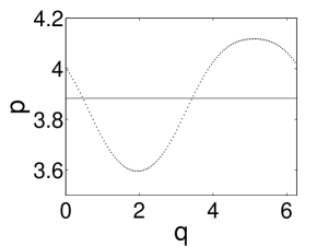
Figure 1: The $\omega=\omega_{g}=3.883\cdots$ golden mean invariant torus of the standard map (17) for $K=0.5$; the straight line represents the initial condition.

Next, we apply the method to a sequence of golden-mean invariant tori with increasing $K$. Numerics indicates that there exists a critical value $\tilde{K}_{c}$ such that when $K<\tilde{K}_{c}$, the fictitious time dynamics converges exponentially, as in (8), but for $K>\tilde{K}_{c}$, it diverges. The critical value $\tilde{K}_{c}$ depends sensitively on the torus discretization $2N$ and the termination value $\Delta$. $\tilde{K}_{c}(N)$ computed for $\Delta=2\times 10^{-6}$ and several values of $N$ is

$2N$	64	128	256	512	1024
$\tilde{K}_{c}(N)$	0.34	0.80	0.93	0.9656	0.9762

The golden-mean critical invariant torus is depicted in Fig. 2(a) for $2N=1024$ points discretization of the torus. Small oscillating structures in the critical torus whose resolution would require higher frequency Fourier components are already visible. The uneven distribution of representative points ($s$ parametrization’s embedding into the $(q,p)$ plane) along the torus indicates the drastically varying stretching rate on the invariant torus close to the breakup kada81 ; shen82 . Our variational method of estimating the critical $K_{c}$ parameter is in agreement with the Greene’s estimate gree79 that the golden-mean invariant torus breaks up at the critical value $K_{c}\approx 0.9716$. Moreover, we find that for large values of $2N$ points discretization of the torus, $\tilde{K}_{c}(N)$ approaches $K_{c}$ approximately as $N^{-1}$.

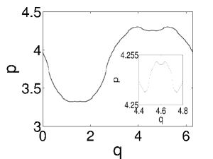
(a)  (b) 

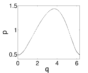
Figure 2: Invariant tori for the standard map (17) for: (a) $\omega=\omega_{g}$ at $K=\tilde{K}_{c}(512)=0.9762$ close to the golden-mean torus critical value $\tilde{K}_{c}$, termination value $\Delta=2\times 10^{-6}$. The inset enlargement of the curve around $q=4.6$ illustrates the fine structure of the nearly critical torus. (b) irrational shift $\omega=2\pi(\pi-3)$ at the estimated critical value $\tilde{K}_{c}(512)=0.4313$, termination value $\Delta=4\times 10^{-6}$. $2N=1024$ torus points discretization.

As Newton descent method does not depend on the specific arithmetical properties of the invariant torus shift, it should work for arbitrary irrational shifts. As an example, we study the family of invariant tori with shift $\omega=2\pi(\pi-3)$. The critical value of convergence of our algorithm is $\tilde{K}_{c}\approx 0.4313$ for $2N=1024$ and $\Delta=4\times 10^{-6}$. The critical torus, depicted on Fig. 2(b) exhibits non-uniform $s$-parametrization and oscillating structure, though much less so than the golden-mean critical torus.

In order to assess the sensitivity of the method to the choice of the termination value $\Delta$, we have studied its influence on the estimation of the critical $\tilde{K}_{c}$. For the golden-mean example, a decrease in the termination value to $\Delta=10^{-6}$ for $\omega=\omega_{g}$ and $2N=1024$ points discretization of the torus, yields $\tilde{K}_{c}=0.6188$ much smaller than the value of $\tilde{K}_{c}=0.9762$ obtained for $\Delta=2\times 10^{-6}$. The corresponding invariant torus for $\Delta=10^{-6}$ is depicted in Fig. 3(a). We notice that this torus looks much smoother than the one obtained for $\Delta=2\times 10^{-6}$ (see Fig. 2(a)). Similarly, for $\omega=2\pi(\pi-3)$ a decrease of the termination value to $\Delta=2\times 10^{-6}$, yields a much smaller critical value $\tilde{K}_{c}=0.3004$. The corresponding invariant torus for $\Delta=2\times 10^{-6}$ is shown in Fig. 3(b). The points are distributed more evenly than in Fig. 2(b), indicating that the invariant torus obtained using this termination value is far from criticality.

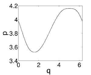
(a)  (b) 

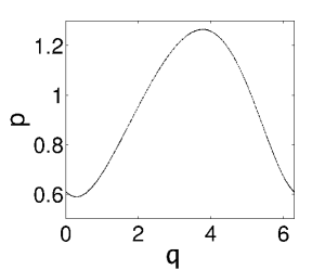
Figure 3: The invariant tori for the standard map (17) with smaller termination values $\Delta$ than in Fig. 2, the same number of torus points $2N=1024$: (a) $\omega=\omega_{g}$ with $\tilde{K}_{c}=0.6188$ and $\Delta=10^{-6}$; and (b) $\omega=2\pi(\pi-3)$ with $\tilde{K}_{c}=0.3004$ and $\Delta=2\times 10^{-6}$.

In summary: For fixed $2N$ points discretization of the torus, if $\Delta$ is too small, then $\tilde{K}_{c}(N)<K_{c}$, while if $\Delta$ is too large, then $\tilde{K}_{c}(N)>K_{c}$. At the threshold of criticality the invariant torus is fractal and thus cannot be resolved by a smooth finite Fourier truncation. The discrepancy between the invariant torus and its numerical discretization has a complicated influence on the fictitious time dynamics, not elucidated in this investigation. If $\Delta$ is too small, the discrepancy leads to an estimate of $\tilde{K}_{c}$ lower than the true $K_{c}$, making the torus appear smoother. If $\Delta$ is too large, the discretization will average out the small features, converging to a grid beyond the critical value. With increasingly refined $2N$ point-discretization of the torus, the value of $\Delta$ needs to be chosen carefully in order to improve the $K_{c}$ estimate.

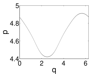
Figure 4: An invariant torus of the standard map (17) for $K=0.352$ obtained by the fictitious time dynamics with the phase condition (12). The method yields shift $\omega\approx 4.67857$. $2N=256$ points discretization of the torus, termination value $\Delta=2\times 10^{-6}$.

So far we have determined invariant tori of the standard map by imposing a constant shift condition (11). An alternative is the phase condition (12) which requires that the motion of representative points along the torus during the fictitious time dynamics averages to zero. In this case the shift $\omega$ is not fixed, but is determined by the fictitious time dynamics. We test this condition by starting with an initial torus ${\bf x}(s)=(s,9\omega_{g}/10)$ discretized on $2N=256$ points, with termination value $\Delta=2\times 10^{-6}$. For $K=0.352$ the Newton descent method yields the invariant torus of the standard map shown in Fig. 4, with shift $\omega\approx 4.67857$.

IV.2 A periodically forced Hamiltonian system

As our second test case, we consider the forced pendulum

$$H(p,x,t)={p^{2}}/{2}-\varepsilon(\cos x+\cos(x-t))\,,$$ (19)

a time-dependent Hamiltonian flow with 1.5 degrees of freedom. $H(p,x,t)$ is a periodic function of the angle variable $x$ and the time variable $t$, with dynamics on $\mathbb{R}\times\mathbb{T}^{2}$. The Poincaré return map for the stroboscopic section $t=0\;\;\mathrm{mod~{}}2\pi$ is a reversible area-preserving map. The Jacobian $J$ required for the fictitious time dynamics (9) is evaluated by integrating

$$\dot{J}=AJ\,,\;A=\left(\begin{array}[]{lr}0&1\\ -\epsilon(\cos x+\cos(x-t))&0\end{array}\right)\,,\;J(0)=1\,.$$ (20)

We apply the fixed shift condition (11) Newton descent to the determination of the invariant torus with the golden-mean shift $\omega=\bar{\omega}_{g}=(\sqrt{5}-1)/2$. For the initial guess torus we take the golden-mean torus of Hamiltonian (19) with $\varepsilon=0$, i.e. ${\bf x}(s)=(s,\bar{\omega}_{g})$. We define $\tilde{\varepsilon}_{c}(N)$ to be the minimum value of the parameter of the model at which the algorithm defining the fictitious time dynamics with $2N$ sampling points fails to converge at fixed $\Delta$. The critical values $\tilde{\varepsilon}_{c}(N)$ computed for different numbers of sampling points (termination value $\Delta=2\times 10^{-6}$) are

$2N$	64	128	256	512	1024
$\tilde{\varepsilon}_{c}$	0.01688	0.02312	0.02594	0.02750	0.02781

For $2N=512$ and $2N=1024$ the $\tilde{\varepsilon}_{c}(N)$ values that we find are are close to the threshold $\varepsilon_{c}\approx 0.02759$ estimated in Ref. PRchan . The invariant torus with $\varepsilon=0.02781$, $2N=1024$ and $\Delta=2\times 10^{-6}$ shown in Fig. 5(a) exhibits non-smoothness and an uneven distribution of discretization points characteristic of criticality. Setting $\Delta=10^{-6}$ leads to the invariant torus with the critical value estimate $\tilde{\varepsilon}_{c}=0.01844$, displayed in Fig. 5(b). It looks smooth, indicating that it is far from criticality and thus that the termination value is too small.

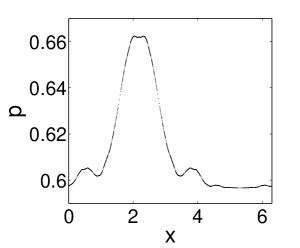
(a)  (b) 

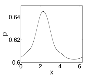
Figure 5: Invariant tori of Hamiltonian (19) with $\omega=\bar{\omega}_{g}$ obtained by the fictitious time dynamics with $2N=1024$ and two different termination values: (a) $\Delta=2\times 10^{-6}$ yields a critical value $\tilde{\varepsilon}_{c}=0.02781$, and (b) $\Delta=10^{-6}$ yield to an underestimate $\tilde{\varepsilon}_{c}=0.01844$.

IV.3 Two coupled standard maps

In principle, the Newton descent method is applicable to determination of invariant tori of arbitrary dimension for flows or maps of arbitrary dimension. In practice, one is severely limited by computational constraints.

In order to test the feasibility of the method in higher dimensions, here we consider two coupled standard maps kan85arn ,

$$I_{n+1} = I_{n}+\epsilon_{1}\sin\theta_{n}+\epsilon_{3}\sin(\theta_{n}+\psi_{n})$$

$$\theta_{n+1} = \theta_{n}+I_{n+1}$$ (21)

$$J_{n+1} = J_{n}+\epsilon_{2}\sin\psi_{n}+\epsilon_{3}\sin(\theta_{n}+\psi_{n})$$

$$\psi_{n+1} = \psi_{n}+J_{n+1}\,,$$

with 4-dimensional phase space, and demonstrate that the method can determine 1- and 2-dimensional invariant tori. The fictitious time dynamics (15) acts on the ${\bf x}=(\theta_{n},I_{n},\Psi_{n},J_{n})$ phase space, with dynamics ${\bf f}({\bf x})$ defined by (21).

First, we apply the fixed shift (18) fictitious time dynamics to determination of the 1-dimensional golden mean invariant torus with shift $\omega=\omega_{g}$. For the initial guess torus we take the integrable case torus $\epsilon_{1}=\epsilon_{2}=\epsilon_{3}=0$ :

$${\bf x}(s)=(s,\omega_{g},s,\omega_{g}).$$ (22)

In the numerical experiment we then search for a typical 1-$d$ invariant torus, for (arbitrarily chosen) small coupling values $\epsilon_{1}=0.1$, $\epsilon_{2}=0.15$, $\epsilon_{3}=0.005$ .

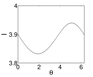
(a)  (b) 

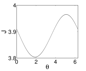
Figure 6: A 1-dimensional invariant torus with shift $\omega_{g}$ of (21) with $\epsilon_{1}=0.1$, $\epsilon_{2}=0.15$ and $\epsilon_{3}=0.005$ : (a) $I-\theta$ projection; (b) $J-\theta$ projection. $2N=512$ points discretization of the torus, termination value $\Delta=10^{-6}$.

The invariant torus obtained by the fictitious time dynamics in this case is shown in Fig. 6. Numerically $\theta=\psi$, indicating that for this 1-dimensional torus the two phases are entrained. The torus appears very smooth, indicating that for the parameter values chosen it is far from the critical values.

Next, we apply the Newton descent to the determination of a 2-dimensional torus with non-resonant frequencies $\omega_{1}$ and $\omega_{2}$. In this case, we need two cyclic parameters $(s_{1},s_{2})\in[0,2\pi]^{2}$ to locate a point on the torus. In (18) we take

$${\bf k}=\left(\begin{array}[]{c}k_{1}\\ k_{2}\end{array}\right),\;{\bm{\omega}}=\left(\begin{array}[]{c}\omega_{1}\\ \omega_{2}\end{array}\right),\;{\bf s}=\left(\begin{array}[]{c}s_{1}\\ 0\\ s_{2}\\ 0\end{array}\right),\;{\bf e}_{1}=\left(\begin{array}[]{cc}1&0\\ 0&0\\ 0&1\\ 0&0\end{array}\right).$$

The initial guess is chosen as in the integrable $\epsilon_{i}=0$ case

$${\bf x}(s_{1},s_{2})=(s_{1},\omega_{1},s_{2},\omega_{2}).$$ (23)

In the numerical experiment we then search for (arbitrarily chosen) $\epsilon_{1}=0.07$, $\epsilon_{2}=0.1$ and $\epsilon_{3}=0.004$ 2-dimensional invariant torus with (also arbitrarily chosen) frequencies $\omega_{1}=\omega_{g}$ and $\omega_{2}=\pi(\sqrt{3}-1)$. In order to reduce the computational time, we take a rather coarse $2N=32$ grid, with $(2N)^{2}=1024$ points representing the torus.

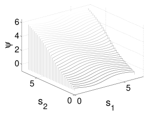
(a)  (b) 

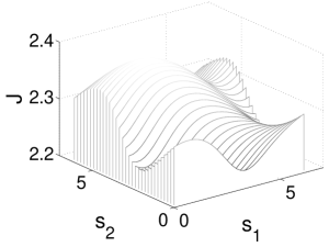
Figure 7: The 2-dimensional invariant torus of the coupled standard maps (21) with incommensurate frequencies $\omega_{1}=\omega_{g}$ and $\omega_{2}=\pi(\sqrt{3}-1)$ for $\epsilon_{1}=0.07$, $\epsilon_{2}=0.1$ and $\epsilon_{3}=0.004$. $(2N)^{2}=1024$ points discretization of the torus, termination value $\Delta=10^{-4}$.

Two projections of the resulting invariant torus for $\Delta=10^{-4}$ termination value are shown in Fig. 7. While the $\psi(s_{1},s_{2})$ and $J(s_{1},s_{2})$ dependence on $s_{1}\,,s_{2}$ shown in Fig. 7 follows in shape the integrable case (23) dependence, the small coupling terms induce significant oscillations. The smoothness of the invariant torus indicates that the parameters are not close to the critical values. For $(2N)^{2}=1024$ points discretization of the torus, $\Delta$ can be as low as $5.1\times 10^{-5}$, and for $(2N)^{2}=4096$, as low as $1.6\times 10^{-5}$. However, the computation takes at least $100$ times longer, and in this exploratory study the larger $(2N)^{2}$ resolutions were out of reach.

IV.4 Kuramoto-Sivashinsky system

In our last example, we apply the Newton descent to determination of an invariant 2-torus embedded in a high-dimensional strongly contracting flow. Special tori that can be converted to periodic orbits in a rotating or moving frame have previously been computed for the complex Ginzburg-Landau equation lop05rel , and for the 2-d Poiseulle flow cas00num . Here we shale determine a generic 2-torus of the Kuramoto-Sivashinsky equation kuturb78 ; siv ; HLBcoh98 parametrized by the system size $L$,

$$u_{t}=(u^{2})_{x}-u_{xx}-u_{xxxx}\,,\qquad x\in[0,L]\,.$$ (24)

The Kuramoto-Sivashinsky equation describes the interfacial instabilities in a variety of contexts, like the flame front propagation, the two fluid model and the liquid film on an inclined plane.

In the study of flame fluttering on a gas ring as the system size $L$ increases, the “flame front” becomes increasingly unstable and turbulent. As shown in Refs. ruell71 ; nhouse78 , in dissipative systems $2$-dimensional tori often result from a Hopf bifurcation while $3$- (or higher-) dimensional tori are a rare occurrence. In the following we restrict our search to the antisymmetric solution space of (24) with periodic boundary conditions, i.e. $u(-x,t)=-u(x,t)$ and $u(x+L,t)=u(x,t)$, with $u(x,t)$ Fourier-expanded as

$$u(x,t)=\sum_{k=-\infty}^{\infty}ia_{k}e^{ikqx},$$ (25)

where $q=2\pi/L$ is the basic wavenumber and $a_{-k}=-a_{k}\in\mathbb{R}$. Accordingly, (24) becomes a set of ordinary differential equations :

$$\dot{a}_{k}=((kq)^{2}-(kq)^{4})a_{k}-kq\sum_{m=-\infty}^{\infty}a_{m}a_{k-m}\,.$$ (26)

In the asymptotic regime of (26) for $k$ large $a_{k}$’s decay faster than exponentially, so a finite number of $a_{k}$’s yields an accurate representation of the long-time dynamics. In our calculation, a truncation at $d=16$ suffices for a quantitatively accurate calculation.

In the current example, $2N=128$ points are used to represent the torus on the Poincaré section $a_{1}=0.06$. Numerical experimentation indicates that for $L=40.95$ trajectories spend significant fraction of time in a toroidal neighborhood, suggesting that a (partially hyperbolic?) invariant 2-torus exists at this system size: Poincaré section returns of a typical orbit fall close to a closed curve. The initial guess for the Newton descent is constructed by choosing 128 points to represent this curve and their Fourier transform is used to initialize the search with (18). In this case the shift $\omega$ is fixed by dynamics, and in order to compute it we impose the phase condition (12).

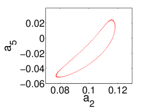
(a)  (b) 

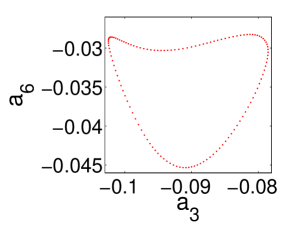
Figure 8: The projections of the 2-dimensional invariant torus of (26) on the Poincaré section $a_{1}=0.06$ with shift $\omega=0.5968$ for $L=40.95$ : Projection on (a) $(a_{2},a_{5})$ and (b) $(a_{3},a_{6})$. The Poincaré section return times are in the range $T=24.18\pm 0.3$. $2N=128$ torus points parametrization, $\Delta=10^{-4}$ termination value.

Fig. 8 shows two Poincaré section projections, in the Fourier space, of the invariant 2-torus of the Kuramoto-Sivashinsky flow determined by the Newton descent method. The method yields the shift $\omega=0.5968$. Even though the invariant torus is very smooth and discretization points are evenly distributed, surprisingly many points are required to resolve the torus. For attempts with fewer discretization points, for example $2N=64$, the search did not converge even with $\Delta=10^{-2}$.

V Summary

We have generalized the “Newton descent” variational method to determination of invariant $m$-tori in general $d$-dimensional dynamical systems, and provided numerical evidence that the method converges in a large domain of existence of invariant tori, up to their breakups. In case of maps and flows with invariant tori such as standard maps, the approach offers an alternative method for determining critical thresholds. While in principle the method is applicable to flows or maps in arbitrary dimension, computation can be expensive for invariant objects larger than 1- and 2-tori. We have utilized the smoothness of the fictitious time evolution to introduce acceleration schemes which improve the efficiency of the method.

In our numerical work, we have implemented the method in the constant shift (4) parametrization, Fourier representation of an $m$-torus. Other discretizations could be better suited to specific applications. For instance, if an invariant torus is close to its critical threshold, representation of small fractal structures requires inclusion of slowly decaying high wavenumber Fourier modes, and a large number of Fourier modes is needed to obtain an accurate representation. Furthermore, the discretization points distribute very non-uniformly when close to criticality. In this limit, other non-constant shift parametrizations of the torus dynamics might be more appropriate. For example, our method is of modest accuracy compared to some of current studies of critical tori, in particular Haro and de la Llave delaLlave04:348 computation of critical tori to 100 digits precision.

In periodic orbit searches we have found the Newton descent approach robust, and very useful for finding periodic orbits in high-dimensional phase-spaces where good guesses for multi-shooting Newton routines are hard to find CvitLanCrete02 ; lanVar1 . Examples worked out here suggest that the method is also a robust starting point for $m$-dimensional invariant tori searches. Once an approximate invariant torus is found by the Newton descent method, it can be used a starting guess for a high precision method, such as some of the currently used Newton’s methods in Fourier space representations of invariant tori.

References

- (1) P. Cvitanović, R. Artuso, R. Mainieri, G. Tanner and G. Vattay, Chaos: Classical and Quantum, ChaosBook.org (Niels Bohr Institute, Copenhagen 2006)
- (2) D. B. Wysham and J. D. Meiss, “Numerical Computation of the Stable and Unstable Manifolds of Invariant Tori”, nlin.CD/0504054, and references therein
- (3) D.V. Treshev, Russian J. of Math. Physics 2, 93 (1994); S.V. Bolotin and D.V. Treshev, Regular and Chaotic Dynamics 5, 401 (2000); INTAS preprint
- (4) M. W. Hirsch, C. C. Pugh and M. Shub, Invariant Manifolds, Lecture Notes in Mathematics V. 583, (Springer-Verlag New York, 1977)
- (5) R. S. Mackay, J. D. Meiss and I. C. Percival, Physica D 13, 55 (1984)
- (6) R. S. Mackay, J. D. Meiss and I. C. Percival, Phys. Rev. Lett. 52, 697 (1984)
- (7) P. Cvitanović, Universality in Chaos (Adam Hilger, Bristol, 1989)
- (8) S. E. Newhouse, D. Ruelle and F. Takens, Commun. Math. Phys. 64, 35 (1978)
- (9) Q. Chen, J. D. Meiss and I. C. Percival, Physica D 29, 143 (1987)
- (10) B. Mestel and I. Percival, Physica D 24, 172 (1987)
- (11) A. Haro and R. de la Llave, “A parameterization method for the computation of invariant tori and their whiskers in quasi periodic maps: rigorous results”, mp_arc 04-348; “A parameterization method for the computation of invariant tori and their whiskers in quasi periodic maps: numerical algorithms”, mp_arc 04-350; “Manifolds at the verge of a hyperbolicity breakdown”, mp_arc 05-96; “A parameterization method for the computation of invariant tori and their whiskers in quasi-periodic maps: numerical implementation and examples”, mp_arc 05-246
- (12) J. Laskar, in C. Simò, ed., Hamiltonian Systems with Three or More Degrees of Freedom, (Kluwer Academic Publishers, Dordrecht, 1999)
- (13) J. Laskar, C. Froeschlé, and A. Celletti, Physica D 56, 253 (1992)
- (14) J. H. E. Cartwright, M. O. Magnasco and O. Piro, Phys. Rev. E 65, 045203 (2002)
- (15) A. Babiano, J. H. E. Cartwright, O. Piro and A. Provenzale, Phys. Rev. Lett. 84, 5764 (2000)
- (16) J. Botina and H. Rabitz, Phys. Rev. Lett. 75, 2948 (1995)
- (17) J.M. Greene, J. Math. Phys. 20, 1183 (1979)
- (18) S. Tompaidis, Exper. Math. 5, 211 (1995)
- (19) R.S. MacKay, Nonlinearity 5, 161 (1992)
- (20) T. S. Parker and L. O. Chua, Practical Numerical Algorithms for Chaotic Systems, (Springer-Verlag New York, 1989)
- (21) C. Simó, in D. Benest and C. Froeschlé, eds., Les Méthodes Modernes de la Mechánique Céleste (Editions Frontiéres, Paris 1990), pp. 285–329. Available on www.dynamicalsystems.org/tu/
- (22) I. G. Kevrekidis, R. Aris, L. D. Schmidt and S. Pelikan, Physica D 16, 243 (1985)
- (23) L. Debraux, hopf bifurcation point”, Contemp. Math. 172, 169 (1994)
- (24) G. Moore, SIAM J. of Numer. Anal 33, 2333 (1996)
- (25) M. van Veldhuizen, SIAM J. Sci. Stat. Comput. 8, 951 (1987)
- (26) H. W. Broer, H. M. Osinga and G. Vegter ZAMP 48, 480 (1997)
- (27) L. Dieci, J. Lorenz and R. D. Russell, SIAM J. Sci. Stat. Comput. 12, 607 (1991)
- (28) H. Mingyou, T. Küpper and N. Masbaum, SIAM J. Sci. Compt. 18, 918 (1997)
- (29) T. Ge and A. Y. T. Leung, Fourier transform approach”, Nonlinear Dynamics 15, 283 (1998)
- (30) F. Schilder. H. M. Osinga and W. Vogt, SIAM J. Appl. Dyn. Syst. 4, 459-488 (2005)
- (31) V. López, P. Boyland, M. T. Heath and R. D. Moser, SIAM J. Appl. Dyn. Syst. 4, 1042 (2005)
- (32) R. L. Warnock and R. D. Ruth, Physica D 26, 1 (1987)
- (33) E. Castellà and À. Jorba, Cel. Mech. and Dynam. Astro. 76, 35 (2000).
- (34) À. Jorba and M. Ollé, Nonlinearity 17, 691 (2004)
- (35) F. Schilder, W. Vogt, S. Schreiber and H. M. Osinga, “Fourier methods for quasi-periodic osillations”, Preprint (2005)
- (36) M. Kaasalainen, Phys. Rev. E 52, 1193 (1995)
- (37) R. L. Warnock, Phys. Rev. Lett. 66, 1803 (1991)
- (38) I. C. Percival, J. Phys. A 7, 794 (1974)
- (39) I. C. Percival, J. Phys. A 12, L57 (1979)
- (40) H-T. Kook and J. D. Meiss, Physica D 35, 65 (1989)
- (41) J. N. Mather, J. Am. Math. Soc. 4, 207 (1991)
- (42) W. E. Gabella, R. D. Ruth and R. L. Warnock, Phys. Rev. A 46, 3493 (1992)
- (43) P. Cvitanović and Y. Lan, in N. Antoniou, ed., Proceed. of 10. Intern. Workshop on Multiparticle Production: Correlations and Fluctuations in QCD (World Scientific, Singapore 2003); nlin.CD/0308006
- (44) Y. Lan and P. Cvitanović, Phys. Rev. E 69, 016217 (2004); nlin.CD/0308008
- (45) H. B. Keller, Numerical Methods for Two-Point Boundary-Value Problems, (Dover, New York 1992)
- (46) J. Stoer and R. Bulirsch, Introduction to Numerical Analysis, (Springer-Verlag, New York 1983)
- (47) W. H. Press, S. A. Teukolsky, W. T. Vetterling, B. P. Flannery, Numerical Recipes in C, (Cambridge University Press, Cambridge, England 1992)
- (48) L. Onsager and S. Machlup, Phys. Rev. 91, 1505 (1953)
- (49) V. I. Arnold, Mathematical Methods for Classical Mechanics, (Spring-Verlag, New York, 1989)
- (50) L.P. Kadanoff, Phys. Rev. Lett. 47, 1641 (1981)
- (51) S.J. Shenker and L.P. Kadanoff, J. Stat. Phys. 27, 631 (1982)
- (52) C. Chandre and H.R. Jauslin, Phys. Rep. 365, 1 (2002)
- (53) K. Kaneko and R. J. Bagley, Phys. Lett. 110A, 435 (1985)
- (54) P. S. Casas and À. Jorba, International Conference on Differential Equations 2, 884 (2000)
- (55) Y. Kuramoto, Suppl. Progr. Theor. Phys. 64, 346 (1978)
- (56) G. I. Sivashinsky, Acta Astr. 4, 1177 (1977)
- (57) P. Holmes, J. L. Lumley and G. Berkooz, Turbulence, Coherent Structures, Dynamical Systems and Symmetry (Cambridge University Press, Cambridge, 1998)
- (58) D. Ruelle and F. Takens, Commun. Math. Phys. 20, 167 (1971)