Scaling properties of $q$-breathers in nonlinear acoustic lattices

Abstract

Recently $q$-breathers - time-periodic solutions which localize in the space of normal modes and maximize the energy density for some mode vector $q_{0}$ - were obtained for finite nonlinear lattices. We scale these solutions together with the size of the system to arbitrarily large lattices. We generalize previously obtained analytical estimates of the localization length of $q$-breathers. The first finding is that the degree of localization depends only on intensive quantities and is size independent. Secondly a critical wave vector $k_{m}$ is identified, which depends on one effective nonlinearity parameter. $q$-breathers minimize the localization length at $k_{0}=k_{m}$ and completely delocalize in the limit $k_{0}\rightarrow 0$.

I Introduction

Spatially extended nonlinear Hamiltonian systems serve as starting models for the study of excitations in many branches in physics, e.g. anharmonic vibrations of crystal lattices, mesoscopic and nanoscopic systems, molecules, but also of electromagnetic, acoustic and other waves in nonlinear media, to name a few. They have been studied over many decades in order to understand such intriguing material properties as heat conductivity, thermal expansion, turbulence, confinement of light, but also general mathematical aspects such as thermalization, mode-mode interactions, etc. While in any realistic situation damping and energy input have to be considered as well, these dissipative effects are often weak enough to allow the observation of the underlying Hamiltonian excitations.

Recently it was shown QB1 , that a one-dimensional anharmonic atomic chain allows for exact time-periodic solutions which localize exponentially in the space of normal modes and have their maximum energy on a mode with mode number $q_{0}$. A $q$-breather, being periodic in time, can be viewed as one normal mode which is dressed by several other normal modes in a neighbourhood of $q_{0}$ and has an infinite lifetime. The existence and properties of these $q$-breathers allowed to explain all major ingredients of the famous Fermi-Pasta-Ulam problem (FPU) fpu ; Ford ; chaosfpu in a clear and constructive way. The FPU problem concerns the nonequipartition of normal mode energies on time scales which can be many orders of magnitude larger than the characteristic vibration periods. The key ingredient for the construction of $q$-breathers is a finite nonlinear system QB1 . This is a very general condition and may apply to many other systems as well. It has been recently successfully tested by considering FPU models with lattice dimension $d=2,3$ QB23D and also discrete nonlinear Schrödinger models (DNLS) in various lattice dimensions QB-DNLS . Further studies also revealed the persistence of $q$-breathers in thermal equilibrium QB1 , which shows their relevance for statistical properties of extended systems. Previous studies of the FPU problem suggested that the effect of nonequipartition will disappear for large system sizes Ford ; chaosfpu . That seems to imply a disappearance of $q$-breathers in that limit. Here we show that $q$-breathers persist and have invariant properties for large system sizes. These results are particularly important because they apply to macroscopic systems.

Consider a generic model of a $D$-dimensional nonlinear lattice of size $N_{1}\times\dots\times N_{D}$, defined by a Hamiltonian

$$H=\sum_{\boldsymbol{n}}\left[\frac{p_{\boldsymbol{n}}^{2}}{2}+U(x_{\boldsymbol{n}})+\sum_{l=1}^{D}V(x_{\boldsymbol{n}+\boldsymbol{e}_{l}}-x_{\boldsymbol{n}})\right]$$ (1)

where $x_{\boldsymbol{n}}$, $p_{\boldsymbol{n}}$ are canonical variables. $U(x)$ and $V(x)$ are anharmonic on-site and interaction potentials, respectively. Their Taylor expansion around $x=0$ starts with quadratic terms. $\boldsymbol{n}=\{n_{1},\dots,n_{D}\}$ is a $D$-dimensional lattice vector with $n_{l}=\overline{1,N_{l}}$. $\boldsymbol{e}_{l}$ denotes a unitary lattice vector along the dimension $l$. Note that $x_{\boldsymbol{n}}=0$ is an equilibrium state of the system. We will consider the case of fixed boundary conditions (BC). We have also studied free and periodic BC with similar results.

This Hamiltonian can be expressed in terms of normal modes $P_{\boldsymbol{q}}$, $Q_{\boldsymbol{q}}$ of the linearized problem, obtained by skipping all anharmonic terms in the potentials:

$$H=\sum_{\boldsymbol{q}}E_{\boldsymbol{q}}+H^{int}(Q_{\boldsymbol{q}})\;,\;E_{\boldsymbol{q}}=\frac{1}{2}\left(P_{\boldsymbol{q}}^{2}+\omega_{\boldsymbol{q}}^{2}Q_{\boldsymbol{q}}^{2}\right)$$ (2)

where $E_{\boldsymbol{q}}$ is the energy of a given normal mode and $H^{int}$ is the mode interaction part of the Hamiltonian which appears due to anharmonicity. The integer components of the mode vector $\boldsymbol{q}$ enumerate the modes. That is a class of models for which exact $q$-breather solutions may exist QB1 ; QB23D . Such solutions are time-periodic and the normal mode energies are exponentially localized around a mode vector $\boldsymbol{q}_{0}$.

We search for a way of scaling a given solution $Q_{\boldsymbol{q}}(t)$ of a system (2) of size $N$ to a solution $\tilde{Q}_{\tilde{\boldsymbol{q}}}(t)$ of a system of scaled size. It consists of scaling the values of mode variables $\sqrt{r}$ times and scaling their indices $r$ times, filling the gaps with zeros:

$${\tilde{Q}}_{\tilde{q}_{l}}(t)=\begin{cases}\sqrt{r}Q_{q_{l}}(t),&\tilde{q}_{l}=rq_{l}\\ 0,&\tilde{q}_{l}\neq rq_{l}\end{cases},$$ (3)

where we omitted all mode indices except the $l$-th component. For fixed BC $q_{l}=\overline{1,N_{l}}$, and the scaled system size is assumed $\tilde{N}_{l}+1=r(N_{l}+1)$. The phase space of the scaled system then possesses an invariant subspace (also coined a bush of modes bushes ). This procedure can be applied to construct a solution to a system of arbitrarily large size, increasing $r$. In order to identify the applicability of (3), we will use a renormalization in real space which is equivalent to (3).

Consider $D=1$ in (1). The equations of motion read

$$\ddot{x}_{n}=f(x_{n})+\varphi(x_{n+1}-x_{n})-\varphi(x_{n}-x_{n-1})\;.$$ (4)

Here $f(x)=-U^{\prime}(x)$, $\varphi(x)=V^{\prime}(x)$ and $\quad n=\overline{1,N}$. For fixed BC $x_{0}=x_{N+1}=0$. We further assume an odd restoring force $f(x)=-f(-x)$. Then (4) is invariant under the following combined parity and sign reversal symmetry: $x_{n}\rightarrow-{x}_{N+1-n}$. The transformation (3) is given by an alternation of spatial blocks, obtained from the previous by parity and sign reversal transform. The blocks are separated by additional nonexcited lattice sites (see Fig. 1):

$$\tilde{x}_{n}(t)=\{{x}_{1}(t),\dots,{x}_{N}(t),0,-{x}_{N}(t),\dots,-{x}_{1}(t),0,\dots\}.$$

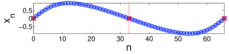
Figure 1: Constructing a solution in a chain of double size in real space. Boundaries and the additional lattice site in the center are marked with crosses. Initial size is N=32. The momentary displacements versus lattice site are shown. (color online)

It is straightforward to observe that if ${x}_{n}(t)$ is a solution to the initial system, then $\tilde{x}_{n}(t)$ is a solution to the scaled-size system. The scaling rule (3) is thus confirmed for 1D chains (4).

We generalize the above results to higher lattice dimensions. The transformation to mode variables is a superposition of 1D transforms. Then, the transformation (3) along a lattice direction $l$ corresponds to the real-space transform already discussed for the $D=1$ case. It yields a solution to a scaled-size system if both $f(x)$ and $\varphi(x)$ are odd functions.

Given a $q$-breather solution for the original finite system, we can thus scale the $q$-breather solution to larger system sizes. Its total energy is scaled in all cases like $\tilde{E}=r{E}$, which is ensured by the block structure of the scaling and the local structure of the coupling in the Hamiltonian (1). The time-dependent mode energies $E_{q}$ are transformed as $\tilde{E}_{\tilde{q}}(t)=r{E}_{q}(t)$ for $\tilde{q}=rq$, and $\tilde{E}_{q}=0$ for other $q$. Introducing the energy density as $\varepsilon=E/(N+1)$ and wave number $k=\pi q/(N+1)$, it is straightforward to observe that the scaling procedure leaves the energy density and the wave number (vector) of a $q$-breather invariant. Together with the rigorous proof of existence of $q$-breathers for finite systems QB1 we arrive at a rigorous proof of existence of these excitations for infinite system sizes, with proper scaling and under certain restrictions for the potential functions. Since the scaled solutions are embedded on mode bushes bushes , the question arises whether $q$-breathers with other (or any) values of $k_{0}$ exist in large systems as well. The fact that the scaling preserves the localization properties of the scaled excitations suggests a positive answer. Below we will address this question. We also note that we needed certain symmetry properties of the potentials for the scaling to work. It however does not imply that for cases with less symmetries $q$-breathers do not exist.

The localization properties of $q$-breathers in the normal mode space have been obtained analytically using asymptotic expansions for FPU-models in various lattice dimensions. For $f=0$ and $\varphi=x+\beta x^{3}$, the result from QB1 ; QB23D is expressed in total energies and mode numbers $E_{(2n+1)q_{0}}=\lambda^{n}E_{q_{0}}$ with $\sqrt{\lambda}=3\beta E_{q_{0}}(N+1)/(8\pi^{2}q_{0}^{2})$ for $D=1$ and $q_{0}\ll N$. We conclude that it must be possible to substitute densities and wave numbers instead, and obtain an expression which is independent of the actual system size. Indeed the outcome of our substitution is written in the following way:

$$\ln\varepsilon_{k}=\left(\frac{k}{k_{0}}-1\right)\ln\sqrt{\lambda}+\ln\varepsilon_{k_{0}},\quad\sqrt{\lambda}=\frac{3\beta}{2^{2+D}}\frac{\varepsilon_{k_{0}}}{k_{0}^{2}}.$$ (5)

Note that these results hold actually for $D=1,2,3$ QB23D . We observe the same scaling properties of (5) as suggested by the real space renormalization procedure from above. Equation (5) implies a smooth dependence of $\lambda$ on $\varepsilon_{k_{0}}$ and $k_{0}$. We thus test whether the scaling can be observed, when the size of the system takes different values, and the new wave number $\tilde{k}_{0}$ is chosen to be the nearest one to the original $k_{0}$ value.

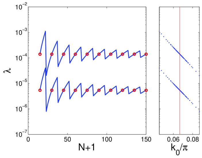
Figure 2: Dependence of the localization parameter $\lambda$ on the system size $N$ of a $q$-breather (left panel) for the $\beta$-FPU chain at constant energy density, $\varepsilon=4\cdot 10^{-4}$ and $2\cdot 10^{-3}$ (for lower and upper curves, respectively) and $\beta=1$. $q_{0}$ is chosen to be the nearest integer to $k_{0}(N+1)/\pi$, $k_{0}=\pi/15$. Open circles mark system sizes $N+1=r(N_{0}+1)$, $N_{0}=15$, for which the prediction is that $\lambda$ should be invariant on the integer $r$. The right panel shows the smooth dependence of the measured $\lambda$ values on the actual wave numbers $k_{0}$ used in the left panel. (color online)

We compute $q$-breathers for that model with $D=1$ for various system sizes starting with $N_{0}=15$ and plot the numerically found $\lambda$ as a function of $N$ in the left panel in Fig.2. The mode number $q_{0}$ is chosen to be the nearest integer to $k_{0}(N+1)/\pi$, $k_{0}=\pi/15$. We obtain $\lambda$ from the ratio of the energy densities $\varepsilon_{5q_{0}}/\varepsilon_{3q_{0}}$. First we observe that $\lambda$ is independent on $N$ when $N+1=r(N_{0}+1)$. Secondly we observe fluctuations of $\lambda$ around a mean value for other values of $N$ due to the fact that for these system sizes the closest wave number to $k_{0}$ will nevertheless be slightly different. These deviations decrease with increase of the system size, and thus the fluctuation amplitude in Fig.2 decreases as well. The piecewise smooth curves show that $\lambda$ depends smoothly on $k_{0}$, since by construction we probe $\lambda$ with wavenumbers slightly varying around $k_{0}$. That is nicely confirmed in the right panel in Fig.2.

Let us analyze the $k$-dependence of (5) for $D=1$. For $q$-breathers at fixed average energy density $\varepsilon$ it follows within the approximation of exponential localization that $\varepsilon_{k_{0}}=(1-\lambda)\varepsilon$. Together with the definition of $\lambda$ in (5) we find, that the inverse localization length in $k$-space is given by the absolute value of the slope $S$:

$$S=\frac{1}{k_{0}}\ln\sqrt{\lambda}\;,\;\sqrt{\lambda}=\frac{\sqrt{1+4\nu^{4}/k_{0}^{4}}-1}{2\nu^{2}/k_{0}^{2}}\;,\;\nu^{2}=\frac{3\beta}{8}\varepsilon\;.$$ (6)

$\lambda$ depends both on $k_{0}$ and $\varepsilon_{k_{0}}$. $S$ vanishes for $k_{0}\rightarrow 0$ and has its largest absolute value $max(|S|)\approx 0.7432/\nu$ at $k_{min}\approx 2.577\nu$. For a fixed effective nonlinearity parameter $\nu$ the $q$-breather with $k_{0}=k_{min}$ shows the strongest localization. Especially for $k_{0}\rightarrow 0$ the $q$-breather delocalizes completely. With increasing $\nu$, the localization length of the $q$-breather for $k_{0}=k_{min}$ increases. For $k_{0}\gg\nu$ it follows $S\approx 2/k_{0}\ln(\nu/k_{0})$ and for $k_{0}\ll\nu$ we find $S\approx-k_{0}/(2\nu^{2})$.

We plot in Fig.3 the dependence $S(k_{0})$ for the $\beta$-FPU chain at three different energy densities.

Figure 3: The slope $S$ as a function of $k_{0}$ for the $\beta$-FPU chain and three different energy densities $\varepsilon=6.08\cdot 10^{-4},9.6\cdot 10^{-4},1.57\cdot 10^{-3}$ and $\beta=1$ (dashed curves, from bottom to top). Symbols and eye-guiding solid lines: estimate of the slope from numerical computations of $q$-breathers for $N=149$ and $N=359$. (color online)

If $\nu$ or $N$ are small enough, then the first nonzero $k_{0}$ value will appear for $k_{0}>k_{min}$. Increasing $\nu$ or $N$ we shift some allowed low lying $k$ values to the left of the minimum $k_{0}<k_{min}$. For very large systems (dense filling of the $x$-axis in Fig.3 with allowed $k_{0}$ values) we thus expect that among them there is an optimum wavelength which provides strongest localization.

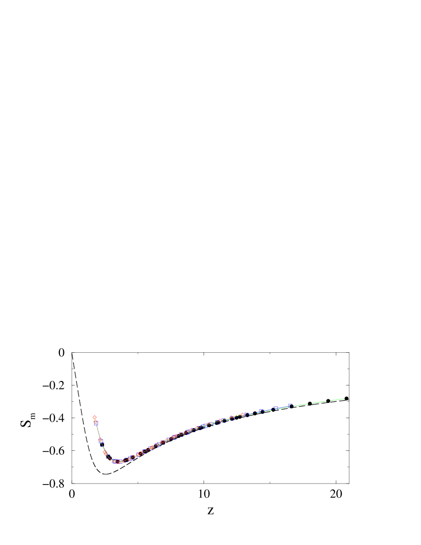
Figure 4: The master slope function $S_{m}(z)$ (dashed line). Different symbols correspond to the numerically obtained slopes from Fig.3 which are scaled accordingly and fall on a single curve. (color online)

We test our prediction by computing the slope for various $q$-breathers of the $\beta$-FPU chain. The results are shown in Fig.3 (symbols).

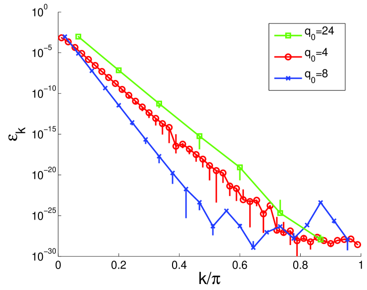
Figure 5: The profiles of $q$-breather solutions for $N=359$, $\beta=1$, $\varepsilon=9.6\cdot 10^{-4}$ and three different values of $q_{0}$ which yield $k_{0}/\pi=0.011,0.022,0.067$ and correspond to the most left point on the middle curve in Fig.3, its minimum and a point to the right of it. Symbols denote the mode energies at the moment of vanishing coordinates $x_{l}=0$. The vertical bars denote the range of mode energy values taken during one period of the $q$-breather. (color online)

We nicely observe an optimum value of $k_{0}$ for localization. Increasing the nonlinearity parameter (by either increasing the nonlinearity strength or the energy density) the critical wavenumber is shifted further away from the edge of the spectrum and gets shallower, as predicted. Deviations from the theoretical curves for small $k_{0}$ are due to strong nonlinear corrections to our estimates, while deviations at larger $k_{0}$ are finite size corrections to the analytical estimates. Note the smooth dependence of $S$ on $k_{0}$ which does not depend on the system size, thus confirming the scaling results from above. We plot in Fig.4 the single master slope function $S_{m}(z)=\nu S$ with $z=k_{0}/\nu$ and scale all numerically obtained slopes as well. The numerical data all condense on one single curve at small $k_{0}$. Thus higher order corrections to the decay law do not alter the scaling properties of $q$-breathers in the limit of small $k_{0}$.

The profiles of three $q$-breather solutions for $\varepsilon=9.6\cdot 10^{-4}$ are shown in Fig.5. The symbols correspond to normal mode energies at the moment when all coordinates vanish. Among them is the $q$-breather with the strongest localization. The precision of computation is $10^{-8}$ (see QB1 for details). Since the normal mode energies are not conserved quantities, we show as well the fluctuation range for each of them. These fluctuations become stronger at particular $k$-values and are possibly due to a closely nearby lying resonance, which nevertheless does not destroy the localization profile.

Let us discuss the obtained results. The reason for the weaker localization of $q$-breathers when $k_{0}\gg\nu$ is the increasing distance $3k_{0}$ between modes excited in consecutive orders of perturbation theory. The delocalization for $k_{0}\rightarrow 0$ however is due to an approaching of resonances $n\omega_{k_{0}}\rightarrow\omega_{k}$ for some integer $n$ QB1 . Note that the same approaching of resonances holds at the upper frequency cutoff where the frequency detuning is quadratic in $k$ and the relevant integer $n=1$. We computed the dependence of the slope $S$ there and obtained a behaviour similar to the one in Fig.3. We expect the above results to qualitatively hold independent of the dimension $D$. It remains a challenging task to perform computations for e.g. $D=2$, since one needs about $10^{5}$ lattice sites, which is presently not reachable with our numerical tools.

We fixed the average energy density in order to ensure finite temperatures. If the energy density $\varepsilon_{k_{0}}$ is fixed, then $q$-breathers will delocalize for some nonzero value of $k_{0}$. For a finite lattice $\varepsilon\approx N\varepsilon_{k_{0}}$ at that point.

We derived similar results for the $\alpha$-FPU model with $\varphi=x+\alpha x^{2}$ using the estimates from QB1 . We obtain strongest localization for $k_{m}\approx 2.39\xi$ and $max(|S|)\approx 1.5/\xi$ with the effective nonlinearity parameter $\xi=\sqrt{\alpha/\pi}\varepsilon^{1/4}$. For small $k_{0}$ the slope $S\sim-(2k_{0}/\xi)^{1/3}$. In all cases the localization becomes meaningless when $|S|^{-1}\approx\pi$ which is the size of the first Brilloin zone. That happens at $\tilde{k}_{0}\approx 3\beta\varepsilon/(4\pi)$ ($\beta$-FPU) and at $\tilde{k}_{0}\approx\alpha^{2}\varepsilon/(2\pi^{5})$ ($\alpha$-FPU). Well defined and localized $q$-breathers exist for $k_{0}\gg\tilde{k}_{0}$. Strong resonances destroy them for $k_{0}\ll\tilde{k}_{0}$ and lead to an effective redistribution of mode energy in that hydrodynamic regime. The same reasoning defines a critical nonlinearity value, for which $k_{m}$ reaches the center of the band. It can be roughly estimated as $\nu,\xi\sim 1$. For larger values of $\nu,\xi$ the system will enter a regime of strong nonlinearity, where $q$-breathers may become meaningless.

We considered standing waves. We expect the results to be also of importance for travelling waves which are reflected at boundaries or inhomogeneities.

We thank Tiziano Penati for stimulating discussions. M.I., O.K. and K.M. appreciate the warm hospitality of the Max Planck Institute for the Physics of Complex Systems. M.I. and O.K. also acknowledge support of the "Dynasty" foundation.

References

- (1) S. Flach, M. V. Ivanchenko and O. I. Kanakov, Phys. Rev. Lett. 95, 064102 (2005); S. Flach, M. V. Ivanchenko and O. I. Kanakov, Phys. Rev. E 73, 036618 (2006).
- (2) E. Fermi, J. Pasta, and S. Ulam, Los Alamos Report LA-1940, (1955); also in: Collected Papers of Enrico Fermi, ed. E. Segre, Vol. II (University of Chicago Press, 1965) p.978; Many-Body Problems, ed. D. C. Mattis (World Scientific, Singapore, 1993).
- (3) J. Ford, Phys. Rep. 213, 271 (1992).
- (4) CHAOS 15 Nr.1 (2005), Focus Issue The Fermi-Pasta-Ulam problem - The first fifty years, Eds. D. K. Campbell, P. Rosenau and G. M. Zaslavsky.
- (5) M. V. Ivanchenko, O. I. Kanakov, K. G. Mishagin and S. Flach, Phys. Rev. Lett., in press; nlin.PS/0604075.
- (6) K. G. Mishagin, M. V. Ivanchenko, O. I. Kanakov and S. Flach, unpublished.
- (7) R. L. Bivins, N. Metropolis, and J. R. Pasta, J. Comput. Phys. 12, 65 (1973); G. M. Chechin, N. V. Novikova and A. A. Abramenko, Physica D 166, 208 (2002); B. Rink, Physica D 175, 31 (2003).