Controlling transitions in a Duffing oscillator by sweeping parameters in time.

Abstract

We consider a high-$Q$ Duffing oscillator in a weakly non-linear regime with the driving frequency $\sigma$ varying in time between $\sigma_{i}$ and $\sigma_{f}$ at a characteristic rate $r$. We found that the frequency sweep can cause controlled transitions between two stable states of the system. Moreover, these transitions are accomplished via a transient that lingers for a long time around the third, unstable fixed point of saddle type. We propose a simple explanation for this phenomenon and find the transient life-time to scale as $-(\ln{|r-r_{c}|})/\lambda_{r}$ where $r_{c}$ is the critical rate necessary to induce a transition and $\lambda_{r}$ is the repulsive eigenvalue of the saddle. Experimental implications are mentioned.

Even the simplest of non-linear dynamical systems, such as those described by second order ODEs are notorious for exhibiting rich phenomenology Strogatz . One of the features of such systems is multi-stability, which strictly exists when all parameters are time-independent. In the case of adiabatically varying parameters, a system initially situated at one of the quasi-fixed points will remain close to it. What happens when the parameters vary faster then the time scales determined by eigenvalues around the fixed points (FP) will be explored here on the case of a damped, driven Duffing oscillator. When the variation of parameters is sufficiently rapid, transitions occur, such that after the rapid variation is finished, the system finds itself at the FP different from the one at which it was initially situated.

Statement of the Problem. We will consider an oscillator obeying the following equation of motion:

$$2f\cos{\phi(t)} = \ddot{x}+2\lambda\dot{x}+\omega_{0}^{2}x\left(1+\alpha x^{2}\right)$$ (1)

$$\dot{\phi} = \gamma(t)$$

where $\omega_{0}$ is the angular frequency of infinitesimal vibrations, $\lambda$ is the damping coefficient, which for a quality factor $Q$ is given by $\lambda=\frac{\omega_{0}}{2Q}$, $\alpha$ is a non-linear coefficient, $f$ is the driving strength, and $\gamma$ is the driving frequency. Upon non-dimensionalizing and re-scaling we obtain the following equation which has the form of a perturbed simple harmonic oscillator:

$$\ddot{x}+x = \epsilon\left(2F\cos{\phi(t)}-\dot{x}-x^{3}\right)$$ (2)

$$\dot{\phi} = 1+\epsilon\sigma(t)$$

For the case of time-independent parameters $F$ and $\sigma$ the amplitude response has the well-known frequency-pulled form  LL ; Nayfeh . For $F>F_{cr}$ there is a region of tri-valuedness with two stable branches and one unstable (middle) branch (Fig. 1). Such response curves have recently been measured for NEMS Ali , indicating their Duffing-like behavior. For a constant $\sigma$ but different $F$ there is also a response function with tri-valuedness for $\sigma>\sigma_{cr}$. To each case there corresponds also a tri-valued phase response (not shown).

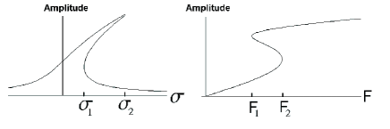
Figure 1: Left: constant $F$. Right: constant $\sigma$.

We would like to explore what happens if the driving frequency, starting from the single-valued region (at $\sigma_{i}$) is rapidly varied in time, into the tri-valued region (ending at $\sigma_{f}$), at a constant F. We will also explore the phenomenology resulting from varying $F$ at a constant $\sigma$ in a similar manner - from a single-valued regime into the tri-valued regime. The variation will take place via a function with a step - either smooth (such as $\tanh$) or piece-wise linear - Fig. 2.

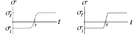
Figure 2: $\sigma(t)$.

In this article we will explore the situation when $F/F_{cr}\sim O(1)$, for instance $F=2F_{cr}$. When $F\sim F_{cr}$, the size of the hysteresis $(\sigma_{2}-\sigma_{1})$ is also of order $1$ and the perturbation method is especially simple. The more complicated case of $F\gg F_{cr}$ (but small enough that r.h.s. of Eq. (2) is still a perturbation over harmonic oscillator equation) may be considered in a future work.

Phenomenology. We discover the following: upon sweeping $\sigma$ from lower values into the hysteresis, depending on other parameters, the solution of Eq. (2) may jump unto the lower branch. The transitions have a peculiar feature of having lifetimes much longer then the slow time scale of Eq. (2) - the damping time-scale of order $\epsilon$.

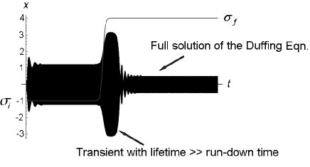
Figure 3: Example of a transition.

Now, there are four relevant ”control knobs”: $F$, $\sigma_{i}$, $\sigma_{f}$ and $r$ defined here as $1/($sweeping time$)$. Consider a set of imaginary experiments, each experiment performed for a different sweep rate $r$, with all three other parameters fixed. As $r$ gets larger, depending on the value of other parameters there may be a critical sweep rate $r_{cr}$ beyond which transitions will be induced. Moreover for $r$ approaching very close to $r_{cr}$ the life-time of transitions, $\tau$, will grow. We will sample these lifetimes and $r-\sigma_{f}$ configuration space numerically and explain the finding theoretically below. However one more observation, depicted in Fig. 4 is in order. For $r$ close to $r_{cr}$, not only do the life-times, $\tau$ of transients tend to grow, but also the amplitudes and phases of these long transients tend to approach that of the middle (unstable) branch of the static Duffing oscillator.

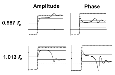
Figure 4: Solutions kiss the unstable branch - envelope of the full numerical solution of Eq. (1) along with quasi fixed points (solutions to Eq. (3)-(4) below with lhs set to $0$) are shown. The function $\sigma(t)$ is displayed as a dotted curve.

We learn that for $r$ close $r_{cr}$ the solution moves unto the unstable branch, lives there for a time period $\tau$ and then either moves unto the top branch if $r<r_{cr}$ or performs the transition unto the bottom branch if $r>r_{cr}$. The jump unto either the top or the bottom branch takes place long after reaching the static conditions (see Fig. 3). A numerical experiment performed at particular parameter values (see Fig. 5) demonstrates the typical situation: plotted on the semi-log plot, the life-time versus $|r-r_{c}|$ nearly follows a straight line. Thus, we learn that $\tau\propto-\ln\left|r-r_{c}\right|$.

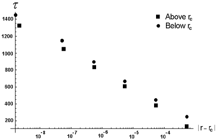
Figure 5: Transient lifetime versus $|r-r_{cr}|$ for $F\approx 2.8F_{cr}$, $\sigma_{i}=-2$, $\sigma_{f}=0.5(\sigma_{1}+\sigma_{2})$

Another numerical experiment was performed to measure $r_{c}$ versus $\sigma_{f}$ for $F\approx 2.8F_{cr}$ and $\sigma_{i}=-2$ (see Fig. 6).

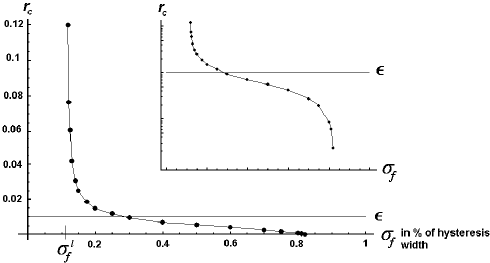
Figure 6: $F=2.8F_{cr}$, $\sigma_{i}=-2$. There is a singularity at $\sigma^{l}_{f}$. The size of the hysteresis was calculated with the first-order theory and therefore it is an over-estimation - the point where $r_{c}$ goes to zero (i.e. at infinitessimal sweep rates) is the exact right edge of the hysteretic region. The existence of singularity at $\sigma^{l}_{f}$ is a genuine effect, since the first-order theory predicts the lower end of the hysteresis more accurately.

Two interesting features are immediately observed: (i) the critical rate necessary to induce a transition is not simply determined by the small parameter $\epsilon$ in the Eq. (2); (ii) when sweeping not deeply enough into the tri-valued region no transitions can be induced for any value of the sweep rate. Increasing $\sigma_{i}$ moves the singularity of $r(\sigma_{f})$ to larger values and varying $F$ does not significantly affect the shape of the $r(\sigma_{f})$ curve. It is somewhat surprising to see singularities in this rather simple problem, especially before the onset chaotic regime. Transitions may occur by sweeping $\sigma$ down; also by sweeping $F$ and holding $\sigma$ constant. Transition phenomenon persists for $F$ large enough that the hysteresis is large (see note in Discussion below).

Theory for small $\Delta\sigma$ case. The regime of $F/F_{cr}\sim O(1)$ guarantees that $(\sigma_{2}-\sigma_{1})\sim O(1)$, thus if $\sigma_{i}$ is chosen sufficiently close to the hysteretic region, the jump in frequency during the sweep, $\Delta\sigma$ is also $\sim O(1)$. This paves way for a simple perturbation method. For example, we write the ”multiple-scales” perturbative solution to Eq. (2) as $X=X_{0}(t,T,...)+\epsilon X_{1}(t,T,...)+O(\epsilon^{2})$ where the slow time scale $T=\epsilon t$, and in general $T^{(n)}=\epsilon^{n}t$. Plugging this into the equation and collecting terms of appropriate orders of $\epsilon$ teaches us that $x_{0}=A(T)e^{it}+c.c.$, i.e. the solution is essentially a slowly modulated harmonic oscillator, with the modulation function satisfying the following Amplitude Equation (AE):

$$Fe^{i\delta(T)}-2i\frac{\partial A}{\partial T}-iA-3\left|A\right|^{2}A=0$$

where $\frac{d\delta}{dT}=\epsilon\sigma(t(T))$. Such AE holds for any sweep rate as long as $\Delta\sigma\sim O(1)$. The AE, broken into real, $x=Re[A]$, and imaginary, $y=Im[A]$, parts are:

$$\frac{dx}{dT} = -\frac{1}{2}x+\sigma(T)y-\frac{3}{2}\left(x^{2}+y^{2}\right)y$$ (3)

$$\frac{dy}{dT} = -\sigma(T)x-\frac{1}{2}y+\frac{3}{2}\left(x^{2}+y^{2}\right)x-\frac{F}{2}$$ (4)

These AE are well known and appear in similar forms in literature Nayfeh ; BM . For a certain range of parameters these equations give rise to a two-basin dynamics with a stable fixed point (FP) inside each basin. The basins are divided by a separatrix which happens to be the stable manifold of the unstable FP of saddle type.

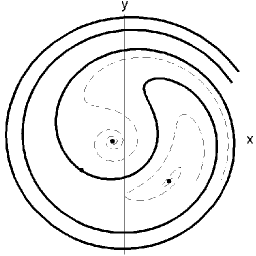
Figure 7: AE dynamics - an example. Typical solutions are shown as dashed curves. Black dots indicate fixed points.

Such basins have recently have been mapped for a certain type of NEMS BasinMapping . Next, consider a set of thought experiments, each sweeping $\sigma$ at a different sweep rate $r$. Immediately after the sweep, the system will find itself somewhere in the two-basin space corresponding to conditions at $\sigma_{f}$, call it a point $(x_{f}(r),y_{f}(r))$. If $(x_{f}(r),y_{f}(r))$ lies in the basin which has evolved from the basin in which the system began before the sweep then there will be no transition. If $(x_{f}(r),y_{f}(r))$ lies in the opposite basin, then that corresponds to a transition! For very low $r$, during the sweep the system will follow closely to the quasi-FP and there will be no transition. In the opposite extreme - infinite $r$, at the end of the sweep the system will not have moved at all, due to continuity of a dynamical system. This endpoint of $\{(x_{f}(\infty),y_{f}(\infty))\}$ may lie in either basin depending on the $\sigma_{f}$.

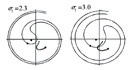
Figure 8: Real examples at $F=2.8F_{cr}$, $\sigma_{i}=-2$. The locus $\{x_{f},y_{f}\}$ is shown by dotted curves.

In the numerical experiments that we considered the first point of the $\{(x_{f}(r),y_{f}(r))\}$ curve to cross the separatrix happens to be this tail at $r=\infty$. This explains the singularity mentioned earlier (see Fig. 6).

Calculation of lifetimes. The point $(x_{f}(r),y_{f}(r))$ serves as an initial condition for subsequent evolution at fixed $\sigma_{f}$. The $(x_{f}(r),y_{f}(r))$ close to the separatrix (i.e. for $r$ close to $r_{c}$) will flow towards the saddle and linger around it for a while. Because this lingering will take place close to the saddle, the linearized dynamics around the saddle should be a good approximation: $\mathbf{r}(T)=\delta l\mathbf{v}_{r}e^{\lambda_{r}T}+R\mathbf{v}_{a}e^{\lambda_{a}T}$, where, for example, $\mathbf{v}_{r}$ and $\lambda_{r}$ are a repulsive eigenvector and eigenvalue, $\delta l$ is the distance of $(x_{f}(r),y_{f}(r))$ away from the separatrix along $\mathbf{v}_{r}$ and R is the characteristic radius of linearization around the saddle. The times at which the system crosses this circular boundary is given by $R=\sqrt{\mathbf{r}\cdot\mathbf{r}}$. The first time, $T_{in}$, is of the order of $\delta l$. The second time is $T_{out}\approx\frac{1}{\lambda_{r}}\ln{\left(\frac{R}{\delta l}\right)}$ (neglecting effects of $\mathbf{v}_{r}$). The lingering time is $\tau=T_{out}-T_{in}\approx T_{out}$. So,

$$\tau=-\frac{1}{\lambda_{r}}\ln{\left(\frac{\delta l}{R}\right)}=-\frac{1}{\lambda_{r}}\ln{\left(\frac{\frac{dl}{dr}|r-r_{c}|}{R}\right)}$$ (5)

Thus we capture the logarithmic dependence of the transient time versus $|r-r_{c}|$.

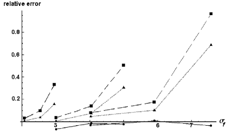
Figure 9: Dotted lines: Fractional errors between the slope of $\tau$ vs. $\ln|r-r_{cr}|$ from exact Duffing and $1/(\epsilon\lambda_{r})$ where $\lambda_{r}$ are computed using the first order perturbation theory in $\epsilon$ (Eqns. (2)-(4)). Dashed lines: same comparison but with $\lambda_{r}$ computed to second order. In both cases, $F=1.5$, $F=2$, $F=2.5$ from left to right. Solid lines: the comparison of $1/(\epsilon\lambda_{r})$ with the same slope from the AE, not full Duffing (only for $F=2$ and $F=2.5$) - remaining errors may be due to inexactness of linearized approximation and omission of $\mathbf{v}_{r}$.

We found that calculating the eigenvalues $\lambda_{r}$ using the second order theory as described in BM systematically lowers the discrepancy in the slope of $\tau$ vs. $|r-r_{cr}|$ computed from exact Duffing and theoretical predictions, Fig. 9, which leads us to conclude that the errors are due to inexactness of the first order AE, not due to the incorrectness of the explanation of the cause of the transition phenomenon.

Experimental Significance. One can propose to use the transition phenomenon with its long transients to position Duffing-like systems unto the unstable (middle) branch (see Fig. 1) - the desire to do this has been expressed by workers in the NEMS community HenkUnstBr . The first question is whether a necessary $r_{c}$ is attainable. We see from Fig. 6 and related discussion that for a vast range of parameters $r_{c}$ is less then $0.1$. Recall that in this paper $r$ is defined simply as $1/($sweep time$)=1/\Delta T$. The more experimentally relevant quantity is $\Delta\sigma/\Delta T$. In the present paper we are concerned with hysteresis widths of order $1$, so $\Delta\sigma$ in question is $\sim 10$ or less. Hence $\Delta\sigma/\Delta T$ necessary to create a transition is, for a vast range of parameters, less then $1$ resonant widths per run-down time (but close to the high-end of the hysteresis this figure falls rapidly - see Fig. 6), which in conventional units corresponds to the sweep rate of $(\omega_{0}/Q)^{2}$ $Hz/sec$. One can also use this as a guide to prevent unwanted transitions in experiments in which $\sigma$ depends on time. The second question is how small must $|r-r_{c}|$ be to induce a transient of time $\tau$. From Eq. (LABEL:eqn:Eq5) we see that $|r-r_{c}|\approx\frac{\omega_{0}}{Q}(dr/dl)\times\exp{\left[-\tau\lambda_{r}(\sigma_{f},F)\right]}$ sec^-1. For any $F$, $\lambda_{r}$ reaches maximum approximately in the middle of the hysteresis where $\lambda_{r}(\sigma_{f}=\frac{\sigma_{2}+\sigma_{1}}{2},F)\approx 0.64(F-F_{cr})/F_{cr}$. So the smaller the $F$, the easier it is to attain a longer transient. The quantity $dr/dl$, at the point of crossing the separatrix diverges at $\sigma_{f}=\sigma^{l}_{f}$ and becomes small ($<1$) for $\sigma_{f}$ close to $\sigma_{2}$ (this explains why the life-time $\tau$ is very sensitive to $|r-r_{c}|$ in this region (see Eq. (5)). The functional form of $dr/dl$ versus parameters is not fundamental - it depends on the form of the ramping function, for example, and can be computed from the set $\{x_{f}(r),y_{f}(r)\}$.

Discussion. Our theoretical hypothesis claims that the point at which the system finds itself at the end of the ramp, $(x_{f},y_{f})$ determines whether there will be a transition or not. However one may be inquire whether this set of points does not consistently cross the separatrix in some special way, for example, always tangentially or always perpendicular to the separatrix. If it does, there must be something happening during the ramp that situates these final points in this special way. Then the theory based on just the final position $\{(x_{f},y_{f})\}$, although is true, would be incomplete. This issue may be addressed in a future work by analyzing the effect of a generic perturbation of either the ramping function or the system on $\{(x_{f},y_{f})\}$. This might also pave the way to understanding the generality of the phenomenon - whether it holds in a large class of two-basin models and ramping functions. Also, we would like to explore the phenomenology for large $\Delta\sigma$ case when the AE (3)-(4) do not hold, yet the system is still in a weakly non-linear regime.

The author thanks Professor Baruch Meerson for suggesting this problem and for ideas and time spent in subsequent discussions and Professor Michael Cross for pointing out the usefulness of thinking about the set $\{(x_{f},y_{f})\}$ and its behavior, as well as for general advice. We acknowledge the support of the PHYSBIO program with the funds from the European Union and NATO as well as the NSF grant award number DMR-0314069.

References

- (1) S. Strogatz, Nonlinear Dynamics and Chaos, Addison Wesley, (1994)
- (2) L. Landau and Y. Lishitz, Mechanics, Addison-Wesley Pub. Co.,(1960)
- (3) A. H. Nayfeh and D. T. Mook, Nonlinear Oscillations, Wiley (1979)
- (4) A. Husain et. al, Appl. Phys. Lett., 83, 1240 (2003)
- (5) Bogoliubov, N.N. and Mitropolsky, Y.A., ”Asymptotic Methods in the Theory of Nonlinear Oscillations”, Gordon and Breach Science Publishers 1961.
- (6) H. W. Ch. Postma et. al., To be submitted
- (7) H. Postma, I. Kozinsky, Private Communication