A spatially extended model for residential segregation

Abstract.

In this paper we analyze urban spatial segregation phenomenon in terms of the income distribution over a population, and inflationary parameter weighting the evolution of housing prices. For this, we develop a discrete, spatially extended model based in a multi–agent approach. In our model, the mobility of socioeconomic agents is driven only by the housing prices. Agents exchange location in order to fit their status to the cost of their housing. On the other hand, the price of a particular house changes depends on the status of its tenant, and on the neighborhood mean lodging cost, weighted by a control parameter. The agent’s dynamics converges to a spatially organized configuration, whose regularity we measured by using an entropy–like indicator. With this simple model we found a nontrivial dependence of segregation on both, the initial inequality of the socioeconomic agents and the inflationary parameter. In this way we supply an explanatory model for the segregation–inequality thesis putted forward by Douglas Massey.

Mathematics Subject Classification: 91D10, 91B72

1. Introduction

The spatial structure of a city is the result of a wide and complex set of factors. The way in which different economic activities and social groups spread over the urban space is the matter of different and complementary theories in Sociology, Geography, Politics and Economy [5, 9, 15, 34]. Housing patterns can be understood as the result of the complex interrelationship between individuals’ actions constrained by social, political and economical rules [9, 36]. Residential segregation is the degree to which two or more groups live separately from one to another in different parts of the urban space [19, p. 282]. This phenomenon is concurrent to several social problems as the concentration of low opportunities to get a well earned job, low scholar development in children of segregated areas, premature parenthood between young people, and the emergence of criminality [21, 22].

Residential segregation has been the subject of extensive research in social sciences for many years. It is a multifactorial phenomenon mainly determined by socioeconomic factors like race and income distribution, as well as factors associated to the structure of the urban space [7, 13, 17, 21, 22].

There are two main quantitative approaches to segregation, the phenomenological one, which relies on segregation measures and indexes [10, 12, 19, 23], and the theoretical one, based on computational or mathematical models [3, 14, 25, 17, 18, 20, 21, 22, 30, 31, 32, 28].

In this paper we propose a spatially extended model based in ideas of Portugali [28] and Schelling [30, 31, 32], to study the relationship between income inequality and residential segregation. The basic thesis proposed by Massey and colleagues [21] is that the degree of spatial segregation experienced by a society increases with its level of inequality. This relationship has been reformulate by Morrison [24] as the segregation–inequality curve.

The organization of the article is as follows. In the next section we briefly expose the main theoretical studies concerning the residential segregation, emphasizing only the ideas and concepts that are relevant to our research. In section 3, we present the mathematical model and the tools needed to analyze our numerical simulation, which we do in section 5. Previous to this, in section 4 we study of asymptotic behavior of the model, and derive some theoretical estimates which we consider for the numerical study. Finally, we conclude with a discussion about the potential of our model as an explanation tool.

2. The segregated city

Residential segregation is a complex phenomenon with several dimensions of analysis, whose governing mechanisms are hard to identify. In a first approximation we can however assume that the phenomenon is governed by a set of structural and behavioral rules which determine the possibility of one individual to get a particular kind of house in a specific location of the city. Since those rules are no evident, simplifying hypotheses are required.

One point of view, based in human ecology, postulates that residential segregation occurs because individuals in a city are in mutual competition for the space and its resources. According to this approach, competition is the main force driving the residential segregation [9, p.86]. The outcome of this competition is determined by the ability of individuals to struggle for advantageous locations in the urban space, i.e. their dominant capacity, which is constrained by sociocultural and socioeconomic rules [9, pp. 85–88].

There are three main hypothesis about the sociocultural rules governing the residential segregation. The first one concerns with the class–selective emigration from poor regions. In a region where coexist both poor and less poor people, the latter tend to emigrate to a more wealthy region. This mechanism tends to isolate and concentrate poor people, increasing in this way the poverty rate of the region. The second hypothesis establishes that neighborhood concentration of poor people reflects the general poverty of the urban area. When the average shows a downward trend, neighborhood poverty rates increase. Finally, the third is related the the racial segregation experienced by poor people. Racial bias causes racial segmentation of the urban housing markets, which concurs with high rates of poverty in specific ethnic groups to concentrate poverty geographically [22, pp. 426–428, and references therein]. These hypotheses are complementary, and were developed to explain segregation in north–american cities, where they have been tested. Perhaps in the Latin–american case racial and sociocultural factors have a less relevant role, making possible to build an explicative model over socioeconomic considerations only.

Taking into account that “markets are not mere meetings between producers and consumers, whose relations are ordered by the interpersonal laws of supply and demand” [15, p. 1], we can formulate socioeconomic rules as market mechanisms. The housing market is formed by two kinds of agents: residents which are interested in the social and individual value or use of the land commodity, and the entrepreneurs which are interested in the exchange value of the land. There is a natural conflict between these two of valuations of land.

There is a set of structural factors that are relevant to housing market dynamics: a) the housebuilding industry; b) the government’s housing policy; c) the structure of the property of land; d) the actual spatial structure of city, i.e. location of labor area, residential areas, and trade–commerce areas; and e) the income structure of the society. The last one has been considered as the most significant for the residential segregation phenomenon. Indeed, Urban Economic theory explains the formation of segregated cities through two main arguments. The first one establishes that a population of households with heterogeneous income competing for the occupation of urban land traditionally results in an income–based stratification of the urban space according to the distance to the city center [1]. The second one links the concentration of low incomes households in some areas, to the existence of local externalities like ethnicity. As a consequence of this, there is a households’ preference to live in relative homogeneous neighborhoods with respect to either income or ethnic similarity [2, 4, 32].

Two levels of analysis may be considered in the study of residential segregation. At the macro level, several structural transformations in the society (changes in income level, tendency to racial exclusion, levels of social integration, etc.) are assumed to determine the spatial concentration of poverty. This is the level of analysis in [7, 13, 16, 22]. At the micro level, specific discriminatory individual behaviors related individual characteristics (sex, age, religion, ethnic group, nationality, etc.) influence the choice of a place to live. This is the point of view in [6, 28, 27, 30, 31, 32], and it is also the one we adopt here.

Our model was developed with the purpose of studying Massey’s thesis [21, p. 400], which relates the degree of spatial segregation experienced by a society, to its inequality degree (income disparity). This thesis was reformulated as the segregation–inequality curve (see Figure 1) by Morrison [24]. More precisely, we intend to determine the relationship between these two quantifiable phenomena, inequality and segregation, in a situation where the whole dynamics is governed basic rules of socioeconomic nature.

Figure 1. Segregation–inequality curve according to Morrison et al. [24]

3. Model Structure

Our model is inspired in the works of Schelling [30, 31] and Portugali et. al [28]. Like Portugali’s models, the physical infrastructure of our “simplified city” is modeled by a two–dimensional lattice of finite size $\Lambda_{m,n}=\{1,2,\ldots,m\}\times\{1,2,\ldots,n\}$. A two–dimensional integer vector $\hbox{\bf x}=(\hbox{\bf x}_{1},\hbox{\bf x}_{2})\in\Lambda_{m,n}$ represent spatial coordinates. At each time step, the price of the house at location x is a positive real number. Each house is occupied by a householders or agent, who can be distinguished only by his/her socioeconomic status. We quantify this status with a real number taking one of three possible values $p<m<r$ (which stands for poor, middle class, and rich respectively). At time $t$, each agent occupies one specific house of the city. Houses are identical in their characteristics but differentiable by their prices.

There are two main mechanism setting up the house’s prices dynamics: the neighborhood influence, and the householder’s economic status. On the other hand, the agents change position subject to availability, under the pressure of their housing situation. Agents can move inside the city to achieve an optimal match between their status and the price of the house they inhabit. Agents try to live in houses with prices, but not too much, that their economic status.

At time $t$, the prices of houses are encoded in a $m\times n$ matrix $V^{t}:=(V^{t}(\hbox{\bf x}))_{\hbox{\bf{\tiny x}}\in\Lambda_{m,n}}$, while the spatial distribution of agents is stored in a $m\times n$ matrix $A^{t}:=(A^{t}(\hbox{\bf x}))_{\hbox{\bf{\tiny x}}\in\Lambda_{m,n}}$ with values in $\{p,c,r\}$. The price of that house at time $t+1$ is given by:

(1) $$V^{t+1}(\hbox{\bf x})=A^{t+1}(\hbox{\bf x})+\lambda\frac{\sum_{|\hbox{\bf{\tiny x}}(1)-\hbox{\bf{\tiny y}}(1)|+|\hbox{\bf{\tiny x}}(2)-\hbox{\bf{\tiny y}}(2)|\leq 2}V^{t}(\hbox{\bf y})}{\#\{\hbox{\bf y}\in\Lambda_{m,n}:\ |\hbox{\bf x}(1)-\hbox{\bf y}(1)|+|\hbox{\bf x}(2)-\hbox{\bf y}(2)|\leq 2\}}$$

The parameter $\lambda$ weights the influence of the mean price on the neighborhood over the house price, and can be thought as an inflationary parameter: the larger $\lambda$ the higher the asymptotic mean value of the houses in the city.

The distribution of the agents at time $t+1$ differs from its distribution at time $t$ only by a single place exchange between two agents of different status, i. e., at time $t$ we randomly choose two sites $\hbox{\bf x},\hbox{\bf y}\in\Lambda_{m,n}$ and define

(2) $$\delta(\hbox{\bf x},\hbox{\bf y}):=\left(A^{t}(\hbox{\bf x})-V^{t}(\hbox{\bf x})\right)^{2}-\left(A^{t}(\hbox{\bf y})-V^{t}(\hbox{\bf x})\right)^{2}+\left(A^{t}(\hbox{\bf y})-V^{t}(\hbox{\bf y})\right)^{2}-\left(A^{t}(\hbox{\bf x})-V^{t}(\hbox{\bf y})\right)^{2}.$$

This quantity should be interpreted as the economic improvement due to the house exchange between agents a locations x and y. At each unite time, only two agents can participate in such a house exchange. We have $A^{t+1}(\hbox{\bf z})=A^{t}(\hbox{\bf z})$ for $\hbox{\bf z}\not\in\{\hbox{\bf x},\hbox{\bf y}\}$ and

(3) $$A^{t+1}(\hbox{\bf x})=\left\{\begin{array}[]{ll}A^{t}(\hbox{\bf y})&\text{ if }\delta(\hbox{\bf x},\hbox{\bf y})>0,\\ A^{t}(\hbox{\bf x})&\text{ otherwise,}\end{array}\right.$$

and similarly for y. The economic improvement due to a house exchange leads to the reduction on the economic tension

(4) $$T(A,V)=|A-V|:=\sqrt{\sum_{\hbox{\bf{\tiny x}}\in\Lambda_{m,n}}\left(A(\hbox{\bf x})-V(\hbox{\bf x})\right)^{2}}.$$

Agents try to minimize economic tension generated by difference between housing price and status. In our model this difference plays the same role as the dissatisfaction or the unhappiness in the Schelling’s model [26, 30].

3.1. Analytical Tools

The segregation–inequality curve gives the relation between two characteristics of the system: inequality and segregation. The income distribution can be interpreted as a probability vector. The proportions of the population in each income group would be the probability for an individual to belong to that income group. With this idea, income inequality can be measure by using Theil’s inequality index [35, pp. 91–96]. Adapting this index to our situation, we define inequality of a $m\times n$ agents’ distribution $A$ as follows:

(5) $$I(A)=\log(3)+\sum_{i=p,m,r}q_{i}\ \log\left(q_{i}\right),$$

where for $i=p,m,r$, $q_{i}=\#\{\hbox{\bf x}\in\Lambda_{m,n}:\ A(\hbox{\bf x})=i\}/(m\times n)$ is the proportion of agents in each income group. The inequality so defined is an entropy–like indicator taking values in the interval $[0,\log(3)]$. The minimum $I$ corresponds to the case where the total population is equally distributed among all the income groups, and maximum to the limit case of a single income group concentrating the whole population. This last limit would be obtained from distributions where a given income group includes most of the population.

The other characteristic we need to determine the segregation curve is the spatial segregation itself. Though measures of segregation have been the subject of several works in sociology [18, p. 283 and references therein], it is more suitable to our approach to quantify this characteristic by using the degree of order of a given spatial distribution. The idea is to associate the maximum degree of order to a spatial distribution which can be easily described, like a single cluster or a periodic distribution. On the other hand, a random distribution would have a low degree of order. We use an image segmentation technique, the bi–orthogonal decomposition, to associate a degree of disorder (the entropy of the bi–orthogonal decomposition), to a given spatial distribution which we treat as an image [8, p. 131]. Thus, to quantify the segregation (ordering) of the city, we compare the entropy of the bi–orthogonal decomposition of the ordered distribution with that corresponding to a random distribution.

The bi–orthogonal decomposition is the bi–dimensional generalization of the Karhunen–Loève transform, but with the advantage that it is sensible to changes in the spatial structure of one image. To a bi–orthogonal decomposition it is associate an entropy, which measures the amount of information of the image [8, p. 133]. The interpretation is that in an orderer image, i. e. an in–homogeneous distribution of pixels showing a spatial pattern, has low entropy, while to a random distribution of pixels corresponds highest entropy.

Consider a $m\times n$ positive matrix $U$, which is supposed to codify an image or a two–dimensional distribution. The associate covariance matrix $Q:=U^{{\dagger}}U$ is symmetric, and hence its eigenvalues $\{\lambda_{i}:\ i=1,\ldots,m\}$ are real, and the corresponding eigenvectors $\{\phi_{i}:\ i=1,\ldots,m\}$ define an orthonormal basis. The bi–orthogonal decomposition allows us to rewrite the matrix $U$ as,

(6) $$U=\sum_{i=1}^{m}\psi_{i}\phi^{{\dagger}}_{i},$$

where $\psi_{i}=U\phi_{i}$ for $i=1,2,\ldots,m$. The contribution of the submatrix $\psi_{i}\phi^{{\dagger}}_{i}$ to the sum is of the order of the corresponding eigenvalue $|\lambda_{i}|$. The information of the matrix $U$ is concentrate in the submatrices associated to eigenvalues with the highest absolute value. For positive $U$, we neglect the largest eigenvalue $\lambda_{1}$, which can be associated to an spatially homogeneous mode. Using the eigenvalue structure of the bi–orthogonal decomposition, we define the information contents of $U$ by

(7) $$H_{\rm BO}(U)=-\sum_{i=2}^{m}p_{i}\ln p_{i}$$

where

(8) $$p_{i}=\frac{|\lambda_{i}|}{\sum_{k=2}^{m}|\lambda_{i}|}.$$

For an agent distribution $A$, the segregation index is

(9) $$S_{\rm BO}(A)={\mathbb{E}}(H_{\rm BO})-H_{\rm BO}(A),$$

where ${\mathbb{E}}(H_{\rm BO})$ is the expected value of $H_{\rm BO}$ with respect to a random distribution of agents in the $m\times n$–dimensional lattice. We have numerically found that ${\mathbb{E}}(H_{\rm BO})\approx\log(3/5\times\min(m,n))$ for $\min(m,n)\leq 1000$.

4. Asymptotic behavior of the model

In order to understand the asymptotic behavior of the model, let us rewrite (1) and(3) in matrix form as follows:

(10) $$V^{t+1} = A^{t}+\lambda DV^{t}$$

(11) $$A^{t+1} = P^{t}A^{t}$$

Where both $V^{t}$ and $A^{t}$ have to be considered as $m\times n$–dimensional vectors, $D$ is the averaging matrix whose action is defined by (1), and $P^{t}$ is a permutation matrix which permutes at most two coordinates. If for the chosen coordinates $\hbox{\bf x},\hbox{\bf y}\in\Lambda_{m,n}$ we have $\delta(\hbox{\bf x},\hbox{\bf y})>0$, then $P^{t}$ is the matrix permuting those coordinates, otherwise $P^{t}$ is the identity matrix.

After a sufficiently large number of iterations, name $T$, the agents achieve a spatial distribution $A^{*}$ which cannot be improved. From that point on, the distribution of housing prices follows the affine evolution $V^{T+t}=A^{*}+\lambda DV^{T+t-1}$, so that

(12) $$V^{T+t}=(\lambda D)^{t}V^{T}+\left(\sum_{s=0}^{t-1}(\lambda D)^{s}\right)A^{*}=(\lambda D)^{t}V^{T}+\left(\hbox{\rm Id}-(\lambda D)^{t}\right)\left(\hbox{\rm Id}-\lambda D\right)^{-1}A^{*}.$$

The long–term distribution of housing prices is therefore $V^{*}:=\left(\hbox{\rm Id}-\lambda D\right)^{-1}A^{*}$, so that the economic tension associate to the asymptotic distribution of agents is

(13) $$T^{*}(A^{*}):=T(A^{*},V^{*})=|A^{*}-\left(\hbox{\rm Id}-\lambda D\right)^{-1}A^{*}|=\lambda\times|\left(\hbox{\rm Id}-\lambda D\right)^{-1}(DA^{*})|.$$

Because of the non–deterministic nature of the evolution of our system, the asymptotic distribution $A^{*}$ is not uniquely determined by initial conditions. Nevertheless, it has to satisfy the following “variational principle”

(14) $$T^{*}(A^{*})=\min_{P}\left|\left(P-\left(\hbox{\rm Id}-\lambda D\right)^{-1}\right)A^{*}\right|,$$

where the minimum is taken over the set of all two–sites permutations. This is equivalent to say that asymptotically no location exchange can diminish the economic tension.

4.1. Critical $\lambda$

For $\lambda$ small, a spatially disordered initial distribution of agents $A^{0}$ remains unchanged, and the system evolves following an affine law, converging to $A^{*}=A^{0},V^{*}=(\hbox{\rm Id}-\lambda D)^{-1})A^{0}$. For each spatially disordered initial distribution $A^{0}$, there exists a critical value $\lambda_{c}$ for which $A^{0}$ evolves towards an spatially organized state $A^{*}$. This distribution is composed by relatively small number of clusters, each one of them consisting of a nucleus of rich agents surrounded by middle class ones, while the lower class agents occupy the space left by the clusters. In our numerical experiments, which we describe below, we have found that $\lambda_{c}$ essentially depends on the proportion of $r$, $m$, and $p$ in $A^{0}$.

A two sites permutation $A^{*}\mapsto PA^{*}$ produces a change in the economic tension

$$T^{*}(A^{*})\mapsto|\lambda\ (\hbox{\rm Id}-\lambda D)^{-1}(DA^{*})+(A^{*}-PA^{*})|.$$

According to Equation (14), this change does not make the economic tension to decrease. In order for this to be so, it is necessary that

(15) $$|PA^{*}-A^{*}|^{2}\geq 2\lambda((\hbox{\rm Id}-\lambda D)^{-1}(DA),PA^{*}-A^{*}),$$

for each two sites permutation $A^{*}\mapsto PA^{*}$. We may decompose $DA^{*}=\overline{A^{*}}\ {\bf 1}+f$, as the sum of a constant vector and a fluctuating one. Since

$$(\hbox{\rm Id}-\lambda D)^{-1}{\bf 1}=\frac{{\bf 1}}{1-\lambda}$$

and $({\bf 1},PA^{*}-A^{*})=0$, then Equation (15) can be written as

$$|PA^{*}-A^{*}|^{2}\geq 2\lambda((\hbox{\rm Id}-\lambda D)^{-1}f,PA^{*}-A^{*}).$$

Taking this into account, we may define $\lambda_{c}$ as,

(16) $$\lambda_{c}=\min\left\{\lambda>0:\ \frac{1}{2}<\max_{P}\frac{\lambda\ ((\hbox{\rm Id}-\lambda D)^{-1}f,PA^{*}-A^{*})}{|PA^{*}-A^{*}|^{2}}\right\},$$

where the maximum is taken over the two–sites permutations. For $P$ interchange coordinates $\hbox{\bf x},\hbox{\bf y}$, we have,

(17) $$\frac{\lambda\ ((\hbox{\rm Id}-\lambda D)^{-1}f,PA^{*}-A^{*})}{|PA^{*}-A^{*}|^{2}}\equiv\frac{((\hbox{\rm Id}-\lambda D)^{-1}f)_{\hbox{\bf{\tiny x}}}-((\hbox{\rm Id}-\lambda D)^{-1}f)_{\hbox{\bf{\tiny y}}}}{2(A^{*}_{\hbox{\bf{\tiny y}}}-A^{*}_{\hbox{\bf{\tiny x}}})}.$$

4.2. An a priori estimate for $\lambda_{c}$

A reasonably good estimate for $\lambda_{c}$ can be obtained as follows. Considering $A^{*}$ as a random field, the Central Limit Theorem ensures that, with very high probability $DA^{*}_{\hbox{\bf{\tiny x}}}\in[\overline{A^{*}}-2\tilde{\sigma},\overline{A^{*}}+2\tilde{\sigma}]$, where

$$\tilde{\sigma}=\frac{1}{\sqrt{N}}\sqrt{{\mathbb{E}}((A^{*}_{\hbox{\bf{\tiny x}}}-\overline{A^{*}})^{2})}.$$

Here $N$ is the number of sites in the computation of the local mean $DA^{*}_{\hbox{\bf{\tiny x}}}$, which in our case is $25$. Hence, with very high probability,

$$\max_{\hbox{\bf{\tiny x}},\hbox{\bf{\tiny y}}}|f_{\hbox{\bf{\tiny x}}}-f_{\hbox{\bf{\tiny y}}}|=4\tilde{\sigma}=\frac{4}{5}\sqrt{\rho_{r}(r-\overline{A^{*}})^{2}+\rho_{m}(m-\overline{A^{*}})^{2}+\rho_{p}(p-\overline{A^{*}})^{2}},$$

where $\rho_{r},\rho_{m},\rho_{p}$ are the proportions of $r,m$ and $p$ in $A^{*}$ respectively. By using the upper bound

$$\max_{\hbox{\bf{\tiny x}},\hbox{\bf{\tiny y}}}|((\hbox{\rm Id}-\lambda D)^{-1}f)_{\hbox{\bf{\tiny x}}}-((\hbox{\rm Id}-\lambda D)^{-1}f)_{\hbox{\bf{\tiny y}}}|\lesssim\frac{\max_{\hbox{\bf{\tiny x}},\hbox{\bf{\tiny y}}}|f_{\hbox{\bf{\tiny x}}}-f_{\hbox{\bf{\tiny y}}}|}{1-\lambda},$$

we obtain

$$\max_{P}\frac{\lambda\ ((\hbox{\rm Id}-\lambda D)^{-1}f,PA^{*}-A^{*})}{|PA^{*}-A^{*}|^{2}}\lesssim\frac{\lambda}{1-\lambda}\times\frac{2\ \sqrt{\rho_{r}(r-\overline{A^{*}})^{2}+\rho_{m}(m-\overline{A^{*}})^{2}+\rho_{p}(p-\overline{A^{*}})^{2}}}{5\ (m-p)}.$$

According to Eq. (16), for $\lambda\geq\lambda_{c}$ we have

$$\frac{1}{2}<\frac{\lambda}{1-\lambda}\times\frac{2\ \sqrt{\rho_{r}(r-\overline{A^{*}})^{2}+\rho_{m}(m-\overline{A^{*}})^{2}+\rho_{p}(p-\overline{A^{*}})^{2}}}{5\ (m-p)}.$$

Taking this into account, we propose

(18) $$\lambda^{*}:=\frac{5\ (m-p)}{4\ \sqrt{\rho_{r}(r-\overline{A^{*}})^{2}+\rho_{m}(m-\overline{A^{*}})^{2}+\rho_{p}(p-\overline{A^{*}})^{2}}+5\ (m-p)}$$

as an estimate for $\lambda_{c}$.

4.3. An priori estimate for $S_{\rm BO}(A^{*})$ at $\lambda_{c}$

Suppose that $A^{*}$ is composed by $N_{c}$ clusters of comparable size, and suppose also that all of them are symmetric with respect to the coordinate axes. In this case $A^{*}$ has a cluster decomposition

(19) $$A^{*}:=\sum_{i=1}^{N_{c}}Q_{i}P_{i}^{{\dagger}},$$

where $Q_{i}P_{i}^{{\dagger}}$ corresponds to the $i$-th cluster. The vectors $P_{i}$ and $Q_{i}$ have a belled form with maximal value at coordinates where the cluster is located. The vectors $\{P_{i}\}_{i=1}^{N_{c}}$ span a vector space of dimension $n_{c}\leq N_{c}$, for which $\{p_{k}\}_{k=1}^{n_{c}}$ is an orthonormal bases obtained from $\{P_{i}\}_{i=1}^{N_{c}}$ by the Gram–Schmidt process. Using this orthonormal base, we can rewrite $A^{*}:=\sum_{k=1}^{n_{c}}q_{k}p_{k_{i}}^{{\dagger}}$, where the vectors $q_{k}$ are obtained form $Q_{i}$ after the change of basis. With respect to this new basis, $A^{*}$ can be considered a random $n_{c}$ dimensional matrix, therefore $H_{\rm BO}(A^{*})\approx\log(2*n_{c}/3)$, and hence

(20) $$S_{\rm BO}(A^{*})\approx\log(\min(m,n)/n_{c}).$$

Let $N_{\rm min}$ be the cardinality of the less numerous class of agents, i. e.,

$$N_{\rm min}=\min_{i=p,m,r}\#\{\hbox{\bf x}\in\Lambda_{m,n}:\ A^{*}(\hbox{\bf x})=i\}.$$

For small values of the inequality index, i. e., for large $N_{\rm min}$, we have numerically found that $n_{c}\approx\sqrt{N_{\rm min}}$. This is consistent with an agents’ distribution $A^{*}$ formed by $N_{c}\propto N_{\rm min}$ clusters, each cluster containing nearly the same number of agents of the less numerous class. The corresponding cluster decomposition would be obtained from a collection $\{Q_{i}\}_{i=1}^{n_{1}}$ of $n_{1}\propto\sqrt{N_{\rm min}}$ bell shaped vectors, and another collection $\{P_{j}\}_{j=1}^{n_{2}}$ of $n_{2}\approx\sqrt{N_{\rm min}}$ nearly orthonormal bell shaped vectors, as

$$A^{*}=\sum_{i=1}^{n_{1}}\sum_{j=1}^{n_{2}}Q_{i}P_{j}^{{\dagger}},$$

In this case we have $N_{c}=n_{1}\times n_{2}\propto N_{\rm min}$, and $n_{c}=n_{2}\approx\sqrt{N_{\rm min}}$. Hence, for low values of the inequality index $I$, we may expect

(21) $$S_{\rm BO}(A^{*})\approx S^{*}:=\log(\min(m,n)/\sqrt{N_{\rm min}}).$$

Note that $N_{\rm min}$ does not determine the value of $I$. If this value is large enough, the variability of $N_{\rm min}$ inside the collection of agents’ distributions with the same $I$ value produces a large dispersion in $S^{*}$. For this reason it is not possible to define $S^{*}$ as a function of $I$, therefore there is not a unique inequality–segregation curve.

5. Numerical Results

We performed a set of numerical experiments in the $n\times n$ lattice, for $n=64$ and $128$. Each lattice node represents a house location in our virtual city, where agents and values of houses are distributed. At time $t$, theses distributions are codified by $n\times n$ real valued matrices. The agent’s matrix $A^{t}$ takes only three values, $r=1$, $m=1/2$ and $p=1/10$, representing the income of rich, middle class and poor agents respectively. The distribution of house prices $V^{t}$ is a positive matrix, which at time $t=0$ takes values in the interval $[0,1]$. Both spatial distributions, $V^{t}$ and $A^{t}$, evolve interrelatedly according to Eqs. (1) and (3). The unevenness of an agent’s distribution $A$ is measured by using Theil’s index $I(A)$ defined in Eq. (5). Since this indicator depends only on the proportions of rich, middle class and poor agents, then $I(A^{t})=I(A^{0})$ for all $t\geq 0$.

Modeling the demographic composition of a city in a developing country, we have considered “demographic scenarios”, i. e., a given number $N_{p}$ of poor, $N_{m}$ of middle class, and $N_{r}$ of rich agents $N_{r}$, such that $N_{r}<N_{m}<N_{p}$. In order to obtain an inequality–segregation curve, we have chosen a one parameter family of demographic scenarios where $N_{p}$ increases from half to the total population, while the ratio $\alpha=N_{r}/N_{m}<1$ is kept constant. In this way we obtain the family of demographic scenarios

$${\mathcal{F}}_{\alpha}:=\{(N_{p},N_{m},N_{r})\simeq(\eta n^{2},(1-\alpha)(1-\eta)n^{2},\alpha(1-\eta)n^{2}):\ 1/2<1\},$$

which we call “regular”. In our numerical simulation we found no qualitative difference among different regular families. Instead, we have contrasted the behavior shown by ${\mathcal{F}}_{\alpha}$, with that of the family of demographic scenarios obtained as follows: for each value of $I$ we choose, among the demographic scenarios with this inequality index, the most probable one subject to the condition $N_{p}<N_{m}<N_{r}$. For this we first consider the uniform distribution in $\{(N_{p},N_{m},N_{r}):\ 1\leq N_{i}\leq n^{3},\ i=p,m,r\}$, then under conditions $\sum_{i=p,m,r}N_{i}=n^{3}$, $N_{p}<N_{m}<N_{r}$, and $I(A^{*})=I$, we distinguish the most probable one with respect to the conditional probability distribution. In this way we obtain a family ${\mathcal{F}}_{\rm mp}$ of demographic scenarios which we call “most probable”.

For the regular family and for each lattice size $n=64$ and 128, we have considered 10 different demographic scenarios. The demographic scenario thus determines the value of the inequality index $I$. These demographic scenarios have been chosen in order to have 10 nearly equally spaced values for $I$ in the interval of possible values $[I_{\alpha},\log(3)]$. Note how the minimum possible value $I_{\alpha}:=\log(3)+1/2\log(1/2)+\alpha/2\log(\alpha/2)+(1-\alpha)/2\log((1-\alpha)/2)$, depends on the parameter $\alpha$ of the regular family. Now, for each demographic scenario we have chosen 5 different values for the parameter $\lambda$ around our estimate $\lambda^{*}$. Once fixed the demographic scenario and the value of $\lambda$, we performed 20 experiments in both, the $64\times 64$ and the $128\times 128$–lattices. The purpose of these experiments was: 1) to determine $\lambda_{c}$ and compared it to our estimate; and 2) to compute the value of the segregation index at $\lambda=\lambda_{c}$. By doing so, we were able to determine a functional relation between the inequality index and the segregation index, which allows us to draw the segregation–inequality curve. The same experimental protocol was implemented for the family of most probable scenarios. In this case we produce 9 demographic scenarios, corresponding to 9 equally spaced values of $I$ in the interval $[0,\log(3)]$.

Each experiment started with spatial distributions $V^{0}$ and $A^{0}$ randomly generated. The entries of $V^{0}$ were always taken independent and uniformly distributed in the interval $[0,1]$, while for $A^{0}$ the agents determining a given demographic scenario were randomly distributed in the lattice. The experiment consisted in the iteration of the evolution rule, Eqs. (1) and (3), until a stationary distribution $A^{*}$ was reached. In Figure 2 we show the asymptotic distributions of agents $A^{*}$, obtained from the same initial condition $A^{0}$ by using 4 different values of $\lambda$. Note how the asymptotic distribution acquires a more regular structure as we increase $\lambda$.

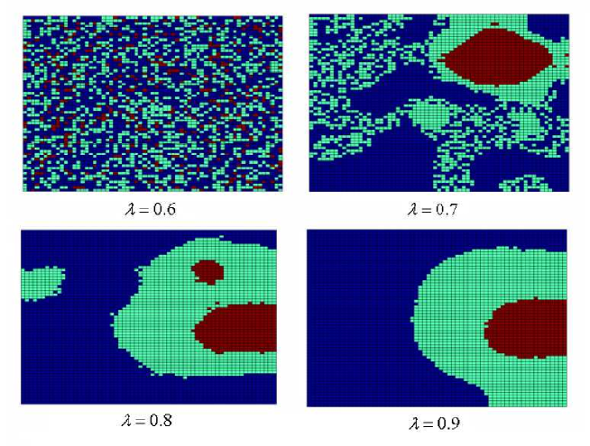
Figure 2. Asymptotic agent’s distribution for different values of $\lambda$ in the $64\times 64$–lattice. Here $I(A^{*})\approx 0.25$ and $\lambda_{c}\approx 0.6$

In order to determine $\lambda_{c}$, for a given initial agents’ distribution $A^{0}$, we compute the evolution of the bi–orthogonal decomposition entropy $H_{\rm BO}(A^{t})$, considering increasing values of $\lambda$. If $\lambda$ is small, $H_{\rm BO}(A^{t})$ remains practically constant along the evolution, while for sufficiently large values of $\lambda$, this entropy undergoes a monotonous decreasing until a definite time that we call segregation time, at which it attains its limiting value. We illustrate this in Figure 3, where we show $H_{\rm BO}(A^{t})$ for $\lambda<\lambda_{c}$ and $\lambda>\lambda_{c}$. Hence, the segregation time may be considered infinite for small values of $\lambda$, and taking finite values for $\lambda\geq\lambda_{c}$. We determine $\lambda_{c}$ corresponding to a initial agents’ distribution $A^{0}$, by computing $H_{\rm BO}(A^{t})$ for $\lambda=\lambda^{*}-0.05,\lambda^{*},\ldots,\lambda^{*}+0.15$, and taking the smallest of these values for which segregation time is smaller than the empirically determined convergence time. The time $T$ an initial configuration $A^{0}$ needs to attain the asymptotic distribution $A*$, increases with both $I(A^{0})$ and $\lambda$. Nevertheless, for the $64\times 64$–lattice and $\lambda<1$, this time never exceeded $1200$ iteration in our simulations. For the $128\times 128$–lattice, this convergence time at $\lambda_{c}$ was always smaller than $2000$, and never exceeded $3200$ for the other values of $\lambda$. The convergence time $T$ appears to increase in proportion to $n\log(n)$, where $n$ is the lattice size.

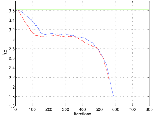
Figure 3. Evolution of the segregation index $H_{\rm BO}(A^{t})$. We show two experiments in the $64\times 64$–lattice, for an agents’ distribution with inequality index $I=0.5$ and $\lambda^{*}\approx 0.68$. The green horizontal line corresponds to $\lambda=0.65$, the blue line was computed with $\lambda=0.75$, and the red was obtained using $\lambda=0.8$.

In Figure 4 we show the behavior of $\lambda_{c}$ as the inequality index changes, for the regular family in the $64\times 64$–lattice, and we compare it to the behavior of our a priori estimate $\lambda^{*}$. In Figure 5 we display the same comparison for to the $128\times 128$–lattice. Since $\lambda^{*}$ depends only on the proportions of rich, middle class and poor agents, it is lattice size independent. According to our numerical results, our a priori estimate is a reasonably tight lower bound for $\lambda_{c}$. Let us remark that the numerical value of $\lambda_{c}$ slightly depends on the initial condition of the experiment, hence we plot the mean value of $\lambda_{c}$ and the corresponding error bars.

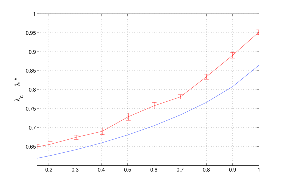
Figure 4. In red $\lambda_{c}$ with its error bars, also as function of Theil’s inequality index $I$. In blue $\lambda^{*}$ also as a function of $I$. Both curves correspond to the regular family, with $\alpha=0.4$, in the $64\times 64$–lattice.

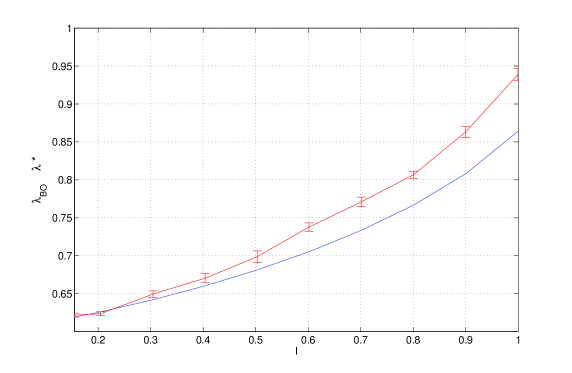
Figure 5. In red $\lambda_{c}$, with its error bars, as function of Theil’s index $I$. In blue $\lambda^{*}$ also as a function of $I$. Both curves correspond to the the regular family, with $\alpha=0.4$, in the $128\times 128$–lattice.

For the family ${\mathcal{F}}_{\rm mp}$, we show in figures 6 and 7 the behavior of $\lambda_{c}$ as a function of the inequality index, in the $64\times 64$ and $128\times 128$–lattices respectively. We compare this to the behavior of our a priori estimate $\lambda^{*}$. Since $\lambda_{c}$ slightly depends on the initial condition, we show $\lambda_{c}$ with the corresponding error bars. Once again, $\lambda^{*}$ is a reasonably tight lower bound for the actual value of $\lambda_{c}$.

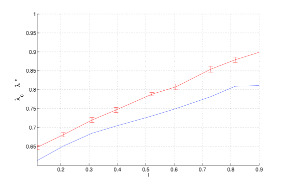
Figure 6. In red $\lambda_{c}$ with its error bars, as a function of $I$. In blue $\lambda^{*}$ also as a function of Theil’s inequality index $I$. Both curves correspond to the the family ${\mathcal{F}}_{\rm mp}$ in the $64\times 64$–lattice.

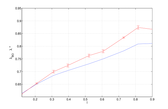
Figure 7. In red $\lambda_{c}$ with its error bars, as a function of Theil’s inequality index $I$. In blue $\lambda^{*}$ also as a function of $I$. Both curves correspond to the family ${\mathcal{F}}_{\rm mp}$ in the $128\times 128$–lattice.

In figures 8 and 9 we plot the segregation index $S_{\rm BO}$ as function of the inequality index, for the regular family in the $64\times 64$ and $128\times 128$–lattices respectively. These are the inequality–segregation curves our model produces. We compare those curves to our a priori upper bound estimate $S^{*}:=\log(n/\sqrt{N_{r}})$ with $n=64$ and 128, which we derived at the end of Section 4. In figures 10 and 11 we plot the same data, corresponding to the family of most probable demographic scenarios. Our numerical results show that, in the case of the regular family, our prediction holds for inequality indices in the interval $0\leq I\leq 0.5$. For the family of the most probable demographic scenarios, the a priori upper bound holds up to $I=0.7$. The exact value of $S_{\rm BO}(A^{*})$ depends on the initial condition $A^{0}$, therefore we show its mean value with the corresponding error bars.

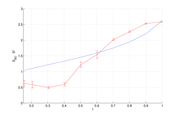
Figure 8. In red the segregation index $S_{\rm BO}$ with its error bars, as function of $I$. In blue $S^{*}=\log(64/\sqrt{N_{r}})$ also as a function of $I$. These inequality–segregation curves correspond the ${\mathcal{F}}_{\alpha}$ family, with $\alpha=0.40$, in the $64\times 64$–lattice.

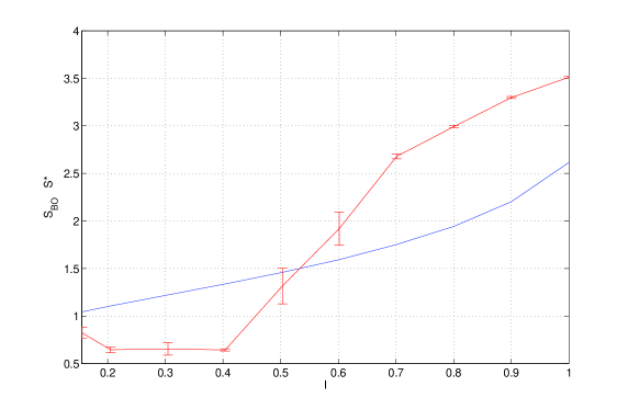
Figure 9. In red the inequality–segregation curve, $S_{\rm BO}$ as function of $I$. Here the segregation index $S_{\rm BO}$ is plotted with its error bars. In blue $S^{*}=\log(128/\sqrt{N_{r}})$ also as a function of $I$. Both curves correspond to the ${\mathcal{F}}_{\alpha}$ family, with $\alpha=0.40$, in the $128\times 128$–lattice.

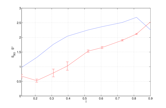
Figure 10. In red the segregation index $S_{\rm BO}$, with the respective error bars, as function of $I$. In blue $S^{*}=\log(64/\sqrt{N_{r}})$ as a function of Theil’s inequality index $I$. Both curves correspond the ${\mathcal{F}}_{\rm mp}$ family in the$64\times 64$–lattice.

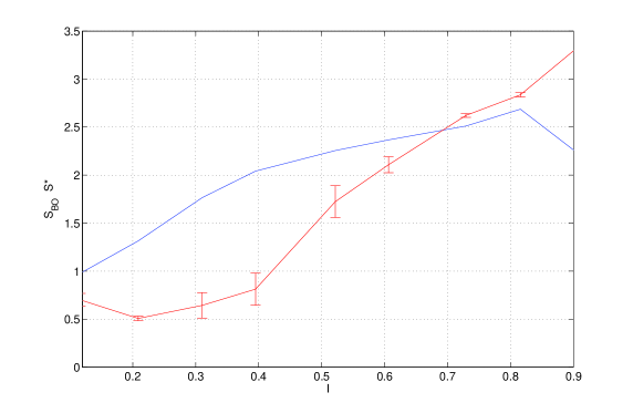
Figure 11. In red the segregation index $S_{\rm BO}$, with the respective error bars, as function of Theil’s inequality index $I$. In blue $S^{*}=\log(128/\sqrt{N_{r}})$ also as a function $I$. Both curves correspond to the ${\mathcal{F}}_{\rm mp}$ family in the $128\times 128$–lattice.

6. Discussion and Conclusions

The model proposed here is intended as a tool towards the explanation of the well–known and accepted thesis of Massey about the relationship between income inequality and spatial distribution of individuals in a city. Build upon basic rules governing the dynamics of house prices and house holders, this model is able to produce spatial patterns whose degree of order grows with the income inequality of the virtual city. Thus we have a mathematical model of segregation, showing a behavior in accordance to the Massey’s thesis. This model introduces a control parameter which we relate to the adjustments of the house prices during the evolution, in a way that segregation occurs only for large enough values of this parameter.

The model does not use a sophisticated housing prices theory, but simple interaction rules similar to those proposed by Portugali and Benenson. Regardless to its validity inside the economic theory, we believe this is a good first approximation for the housing prices dynamics. The mechanism responsible for the segregation is a location exchange process similar the one proposed by Schelling. This process is driven by the economic tension resulting from the difference between the “economic power” of the house holders and prices of the houses they occupy.

Though our model retains many of the Schelling’s ideas, the main difference is nature of the location exchange decision. In Schelling’s original model, this decision is taken based on a satisfaction function that takes in account the number of neighbors of the same kind around a given agent. In our case, an agent decides to exchange is location according to the difference between its income and the price of its house. We think that this is a more realistic situation in the sense that that economic tension can be measure in real life. This mechanism is also better suited for a model of a society where ethnic differences are less determinant than differences imposed by the income.

From the theoretical point of view, the model is interesting by its own. It exhibits an order–disorder phase transition via clustering produced from a very simple exchange mechanism. It also appears to present some finite size scaling behavior which would be pertinent to further explore.

Concerning the indicators we use, Theil’s is a widely accepted inequality index, with the advantage that it is easy to compute and has a direct interpretation. Our segregation index, on the other hand, have never been used in this context. Besides this indicator, we previously tried other entropy–like measures of the degree of order in a spatial distribution, as well as some direct clustering measures. We chose the entropy of the bi–orthogonal decomposition because it is almost as easy to compute as the Theil’s index, and it has a natural interpretation as the information contents of a picture. We are convinced that other segregation measures commonly used in the sociological literature are no suited for our purposes, mainly because they are built from a previous organization of the data, e. g., the census tracks. In our case, the structuration of the urban space is a result only of the location exchange dynamics.

Summarizing, our model is built from a very simple location exchange rule, based on interaction between agents through an economic tension produced by the difference between the agents’ economic capacity and the prices of the houses they occupy. This simple mechanism is sufficient to produce spatial segregation in accordance to Massey’s thesis: segregation is an increasing function of the inequality. With this we were able to furnish key components of an explanatory model of spatial segregation in a situation where the economic factors are more significant than either ethnic or cultural ones.

References

- [1] Alonso, W. Location and Land Use, Harvard University Press, Cambridge, Massachusetts. 1964.
- [2] Benabou, R. (1993). “Workings of a City: Location, Education, and Production”, Quarterly Journal of Economics, Vol. 108 No. 3: (Aug.,1993),
- [3] Benenson, I. “Multi–agent simulations of residential dynamics in the city”, Computer, Environment and Urban Systems, Vol. 22, No. 1. (1998), pp. 25-42.
- [4] Borjas G. “Ethnicity, neighborhood and human-capital externalities”, American Economic Review, Vol. 85, No. 3.(Jun, 1995), pp. 365-390.
- [5] Bourne, L.S. “Urban structure and Land Use Decisions”, Annals of the Association of American Geographers, Vol. 66, No. 4. (Dec., 1976), pp. 531–547.
- [6] Clark, W.A.V. “Residential Preferences and Neighborhood Racial Segregation:A Test of the Schelling Segregation Model”, Demography. Vol. 28, No. 1. (Feb., 1991), pp. 1-19.
- [7] Cloutier, N.R. “Urban residential segregation and black income”, The Review of Economics and Statistics, Vol. 64, No. 2. (May, 1982), pp. 282-288.
- [8] Dente, J.A., Vilela–Mendes, R., Lambert, A. & Lima, R. “The bi-orthogonal decomposition in image processing: Signal analysis and texture segmentation”. Signal Processing: Image Communication 8. (1996) pp. 131-148.
- [9] Duncan, T. The urban mosaic: Towards a theory of residential differentiation. Cambridge University Press, Cambridge, 1971.
- [10] Duncan, O. D. and Duncan, B. “A methodological analysis of segregation indexes”, American Sociological Review, Vol. 20, No. 2. (Apr. 1955), 210-217.
- [11] Farley, Reynolds, et al, 1979, “Barriers to the Racial Integration of Neighborhoods: The Detroit Case”, Annals of the American Academy 441: 97.
- [12] James, D.R. and Taeuber, K.E. (1985) “Measures of segregation”, Sociological Methodology, Vo. 15, 1-32.
- [13] Jargoswky, P.A. “Take the money and run: Economic Segregation in U.S. Metropolitan Areas”. American Sociological Review, Vol. 61, No. 6. (Dec., 1996), pp. 984-998.
- [14] Lieberson, S. and Carter, D.K. “A model for inferring the voluntary and involuntary causes of residential segregation”, Demography, Vol. 19, No. 4. (Nov., 1982), pp. 511-526.
- [15] Logan, J.R., and Molotch, H.L. Urban fortunes: The political economy of place, Berkeley, University of California Press, 1987.
- [16] Massey, D.S. and Fisher, M.J. “How segregation concentrates poverty”, Ethnic and Racial Studies, Vol. 23, No.4. (2000), pp. 670-691.
- [17] Massey, D.S. “Effects of socioeconomic factors on the residential segregation of blacks and Spanish Americans in U.S. urbanized areas”. American Sociological Review, Vol. 44, No. 6. (Dec., 1979), pp. 1015-1022.
- [18] Massey, D.S. and Denton, N.A. “Spatial assimilation as a socioeconomic outcome”, American Sociological Review, Vol. 50, No.1. (Feb., 1985), pp. 94-106.
- [19] Massey, D. S. and Denton, N.A. (1988) “The dimensions of residential segregation”. Social Forces, Vol. 67, No. 2. (Dec., 1988), pp. 281-315.
- [20] Massey, D.S. (1990) “American apartheid: Segregation and the making of the underclass”. The American Journal of Sociology, Vol. 96, No. 2 (Sep.), 329-357.
- [21] Massey, D.S., A.B. Gross and M.L. Eggers 1991 “Segregation, the concentration of poverty, and the life chances of individuals”, Social Science Research 20. (1991), pp. 397-420.
- [22] Massey, D.S., Gross, A.B. and Shibuya, K. “Migration, segregation and the geographic concentration of poverty”, American Sociological Review, Vol. 59, No. 3. (Jun., 1994), pp. 425-445.
- [23] Massey, D.S., White, M. J. and Phua, V. (1996) “The Dimensions of segregation revisited”, Sociological Methods & Research, Vol. 25, No. 2. (Nov., 1996), pp. 172–206.
- [24] Morrison, P.S., P. Callister and J. Rigby “The spatial separation of work–poor and work–rich households in New Zealand 1986-2001: an introduction to a research project”. School of Earth Sciences Research Report No. 17 (Apr., 2003), New Zealand, Victoria University of Wellington.
- [25] Omer., I. “Demographic Processes and Ethnic Residential Segregation”. Discrete Dynamics in Nature and Society, Vol. 3. (1999), pp. 171-184
- [26] Pollicot, M. and Weiss, H. “The dynamics of Schelling–type segregation models and a nonlinear graph Laplacian variational problems” Advances in Applied Mathematics 27. (2001), pp. 17-40.
- [27] Portugali, J. Self–organization and the city. Berlin: Springer-Verlag, 2000.
- [28] Portugali, J., Benenson, I., and Omer, I. “Spatial cognitive dissonance and sociospatial emergence in a self–organizing city”. Environment and Planning B: Planning and Design 27. (1997), pp. 263-285.
- [29] Savage, M. and Warde, A. (1993) Urban Sociology, Capitalism and Modernity. Houndmills: Macmillan Press, Ltd. London.
- [30] Schelling, T.C. “Models of segregation”, The American Economic Review, Vol. 59, No. 2. (May, 1969), pp. 488–493.
- [31] Schelling, T.C. “Dynamic Models of Segregation”, Journal of Mathematical Sociology 1 (1971), pp. 143–186.
- [32] Schelling, T.C. , 1978, Micromotives and Macrobehavior. New York: W.W. Norton.
- [33] Stears, L.B. and Logan, J.R. (1986) “The racial structuring of the housing market and segregation in suburban area”. Social Forces, Vol. 65, No. 1 (Sep.), 28-42.
- [34] Tickamyer, A. R. (2000) “Space matters Spatial Inequality in future sociology”, Contemporary Sociology, Vol. 29, No. 6 (Nov. 2000), pp. 805–813.
- [35] Theil H. Economic and Information Theory. Amsterdam: North Holland, 1967.
- [36] Wilson, A. (2001). Complex Spatial Systems: the modeling foundations of urban and regional analysis. England: Pearson Education Limited. 2001.