Dynamical systems on infinitely sheeted Riemann surfaces

Abstract

This paper is part of a program that aims to understand the connection between the emergence of chaotic behaviour in dynamical systems in relation with the multi-valuedness of the solutions as functions of complex time $\tau$. In this work we consider a family of systems whose solutions can be expressed as the inversion of a single hyperelliptic integral. The associated Riemann surface ${\mathcal{R}}\to{\mathbb{C}}=\{\tau\}$ is known to be an infinitely sheeted covering of the complex time plane, ramified at an infinite set of points whose projection in the $\tau$-plane is dense. The main novelty of this paper is that the geometrical structure of these infinitely sheeted Riemann surfaces is described in great detail, which allows to study global properties of the flow such as asymptotic behaviour of the solutions, periodic orbits and their stability or sensitive dependence on initial conditions. The results are then compared with a numerical integration of the equations of motion. Following the recent approach of Calogero, the real time trajectories of the system are given by paths on $\mathcal{R}$ that are projected to a circle on the complex plane $\tau$. Due to the branching of $\mathcal{R}$, the solutions may have different periods or may not be periodic at all.

Keywords: Complex dynamics, Riemann surface, inversion of hyperelliptic integrals, isochronicity, sensitive dependence.

1 Introduction

It has now become a classical subject to study the connections between the integrability of a dynamical system (or the absence of it) and the singularity structure and multi-valuedness of its solutions. The discovery of this relation dates back to the work of Painlevé and his collaborators [29, 22], who classified all second order ODEs whose solutions have movable poles as their only singularities (now known as the Painlevé property) and are therefore single-valued functions. Then Kowalewskaya found a new integrable case of the heavy top by requiring that the solutions have the Painlevé property [23, 24]. A number of techniques collectively known as Painlevé-Kowalewskaya analysis have been developed over the last thirty years (for a review see, for instance, [31]) to test for this property of the solutions, essentially by seeking for a formal solution near a singularity in terms of a Laurent series, introducing it in the equations and determining the leading orders and resonances (terms in the expansion at which arbitrary constants appear). Painlevé analysis has been extended to test for the presence algebraic branching (weak Painlevé property,[31, 30]) by considering a Puiseaux series instead of a Laurent series. These analytic techniques (which have been algorithmized and are now available in computer packages) constitute a useful tool in the investigation of integrability: in many non-linear systems where no solution in closed form is known, Painlevé analysis provides information on the type of branching the general solution or special families might have. It has also proved to be useful to identify special values of the parameters for which generically chaotic systems such as Hénon-Heiles or Lorenz become integrable.

It is also natural to investigate the singularity structure of solutions of chaotic dynamical systems. Tabor and his collaborators initiated this study in the early eighties for the Lorenz system [32] and the Henon-Heiles Hamiltonian[18]. They realized that the singularities of the solutions in complex-time are important for the real-time evolution of the system. The complex time analytic structure was studied by extensions of the Painlevé analysis involving the introduction of logarithmic terms in the expansion — the so called $\Psi$-series — which provides a local representation of the solutions in the neighbourhood of a singularity in the chaotic regime. Their local analytic approach was complemented by numerical techniques developed for finding the location of the singularities in complex time and determining the order of branching [16]. In all the chaotic systems under study, they observed numerically that the singularities in complex time cluster on a natural boundary with self-similar structure [17]. An analytic argument to explain the mechanism that leads to recursive singularity clustering was given in [26]. Similar studies relating singularity structure, chaos and integrability have been performed by Bountis and his collaborators. Going beyond the local techniques described above, the emphasis was put on a global property of the complex solutions: whether their Riemann surface has a finite or an infinite number of sheets. The authors of [10] proposed to classify the system as integrable in the first case and as non-integrable for the second case.

These ideas actually go back to the work of Kruskal and his poly-Painlevé test to detect non-integrability [25]. Combining analytical and numerical results for a simple ODE, Bountis and Fokas [21] identified a chaotic behaviour with the property that the singularities or branch points of their solutions are dense. In their work, however, it is not too clear whether the criterion is that such points should be dense on the Riemann surface itself or that the projection of the branch points is dense on the complex plane. The second condition is obviously much weaker.

In fact, as was indicated in [1, 2], there exists a wide class of completely integrable Hamiltonian systems whose solutions live on an infinitely sheeted covering of the complex time plane with an infinite number of branch points that are projected onto a dense set on the complex plane and yet are isolated on the covering surface.

Painlevé analysis is a local technique and does not provide information on the global properties of the Riemann surfaces of the solutions (the number and location of the movable branch points, how the different sheets of the Riemann surface are connected together, etc.), which can be important for understanding of the dynamics of the system.

Aware of this limitation, F. Calogero initiated a new line of research by studying the real time dynamics of a system as a path on the Riemann surface of its solution in complex time. In particular, Calogero and Françoise have shown that many isochronous systems can be written by a suitable modification of a large class of complex ODEs [11]. Using local analysis and numerical integration in two many-body systems in the plane [13, 15], it was discovered that the periodic solutions could have a very high period, and the mechanism for the period increase was conjectured. However, in those systems it was not possible to achieve a complete description of the Riemann surface. Although it was proved that all singularities are finite order branch points, the presence of an infinite number of them could still produce aperiodic motion as the solution visits an infinite number of sheets. In the subsequent work [14], the Riemann surface of the solution was infinitely sheeted for generic values of the parameters, yet it could be described in full detail. Using these rather novel techniques, Calogero et al. were able to derive analytic expressions for the periods and prove sensitive dependence on initial conditions. In [14] the projection of square-root branch points of the infinitely sheeted Riemann surface cover densely a circle on the complex plane for generic values of the parameters. As a further step on the way to understand the connection between chaotic behaviour and analytic structure, it was natural to extend the study to Riemann surfaces whose branch points projected onto $\mathbb{C}$ do not cover densely a one-dimensional curve in $\mathbb{C}$, but the whole complex plane. The candidate objects for this study are the Riemann surfaces associated to the inversion of hyper-elliptic integrals, first described by Jacobi [27].

This is precisely the case of the dynamical systems treated in this paper. The text is organized as follows: in Section 2 we introduce a family of simple, generally nonautonomous, dynamical systems whose solutions can be understood as lifting a circular path to a Riemann surface associated to the inversion of a hyperelliptic integral. Global geometrical properties of such surfaces for different cases are described in Section 3. The algorithm that performs the lift of the circular contour on the Riemann surface and possible behaviours of the corresponding solutions are described in Section 4. Here we make a conjecture that all the solutions are either periodic or singular (i.e., they escape to infinity in finite time).

The trajectories of the system for different initial conditions are shown in Section 5, where the path on the Riemann surface is compared with a numerical integration of the equations of motion. Note that trajectories of complex Hamiltonians have been also studied numerically by Bender et al. in [7]. Although the systems they study are different from the ones treated here, their approach is related to the one we propose and the observed complexity of the orbits is similar to the results of Section 5. Finally, conclusions and directions of future work are outlined in Section 6.

2 Two classes of dynamical systems whose solutions travel on the Riemann surface describing inversion of a hyperelliptic integral

In [20] Flashka drew attention to a simple class of integrable Hamiltonian systems in ${\mathbb{R}}^{4}=(x,y,p_{x},p_{y})$ with real time $t$, whose Hamiltonians and additional commuting integrals are given by the real and imaginary parts of arbitrary complex polynomials $H(\zeta,\mu)$, $\zeta=x+iy$, $\mu=p_{x}+ip_{y}$. In contrast to the case of the Liouville integrability, the generic real level surfaces

$${\mathcal{I}}_{E}=\{x,y,p_{x},p_{y}\mid H(\zeta,\mu)=E,E\in{\mathbb{C}}\}$$

are not 2-dimensional tori or products of lines and circles, but algebraic Riemann surfaces with some points removed. Then, instead of straight line motion on the tori, one has flows on such surfaces, which may have a rather complicated behaviour. Solutions of such systems are given by inversion of Abelian integrals on ${\mathcal{I}}_{E}$ and posesses the weak Painlevé property.

Motivated by problems of mechanics and mathematical physics, we restrict ourselves to complex Hamiltonians

$$H=\frac{1}{2}(\zeta^{\prime})^{2}+V(\zeta),$$ (1)

which generate second order complex ODE

$$\zeta^{\prime\prime}=-\frac{dV(\zeta)}{d\zeta}$$ (2)

where $\zeta=\zeta(\tau)$, both $\zeta$ and $\tau$ are complex and the prime denotes differentiation of $\zeta$ with respect to $\tau$.

By fixing the energy, $H=E$, the complex solution is formally obtained as the inversion of the following quadrature

$$\tau-\tau_{0}=\int_{\zeta_{0}}^{\zeta}\frac{d\eta}{\sqrt{2(E-V(\eta))}},$$ (3)

where $\tau_{0}$ is the initial time and $\zeta_{0}=\zeta(\tau_{0})$. Whenever the potential $V(\zeta)$ is a polynomial or a rational function of $\zeta$, the above integral is in general hyperelliptic, and $\zeta(\tau)$ is a multi-valued or even infitely-valued function on the complex plane $\tau$.

We emphasize that a single hyperelliptic integral often appears as a quadrature in various integrable problems of mechanics and mathematical physics, and the last decade the problem of its inversion revokes increasing attention, [1, 3, 19, 33].

On the other hand, by introducing real time $t$ such that $\tau=\varkappa t+\tau_{0}$, $\varkappa$ being arbitrary nonzero complex constant, the real and imaginary parts of $\zeta(\tau(t))$ give a solution of the Hamiltonian system in ${\mathbb{R}}^{4}=(x,y,p_{x},p_{y})$ with a real Hamiltonian proportional to $\mbox{Re}\,\varkappa\mbox{Re}H+\mbox{Im}\varkappa\,\mbox{Im}H$ and describe flows on the hyperelliptic curve $H(\zeta,\mu)=E$.

Some properties of such flows were studied in [4] and, from the algebraic topology point of view, in [28] (see also references therein).

In our paper we focus on a similar yet different class of systems that describe not straight-line, but circular motion on the complex plane $\tau$.

Calogero’s circular motion

F. Calogero has shown that a large class of complex ODEs can be modified in such a way that the resulting system posseses a large number of periodic solutions [12]. Following Calogero’s approach, let us construct another class of systems associated to the quadrature (3) by performing the following change of independent and dependent variables,

$$\tau-\tau_{0} = \frac{1}{{\rm i}\omega}\,\left({\rm e}^{{\rm i}\omega t}-1\right),$$ (4)

$$\zeta(\tau) = {\rm e}^{{\rm i}\alpha\omega t}\,z(t),$$ (5)

where $\omega>0$ is a real parameter that plays the role of a frequency to which the fundamental period $T=2\pi/\omega$ is associated and $\alpha\in\mathbb{R}$ is a parameter still to be determined. The effect of the transformation (5) is to introduce the real time evolution as a parametrization of a circle in the complex $\tau$-plane. Thus the name circular motion as opposed to the straight line motion studied by Flaschka. If the solutions of the complex ODE were analytic or meromorphic functions of $\tau$, then the resulting real time evolution would be periodic, but if the solutions are multi-valued functions of $\tau$ (possibly infinitely-valued) more complex behaviours are possible.

In what follows, for the sake of simplicity, we concentrate on the case

$$V(\zeta)=\zeta^{k+1},\qquad k\in\mathbb{Z}^{+}.$$

The restriction of $V(\zeta)$ to a single power rather than an arbitrary polynomial is by no means essential for the analysis of the geometrical properties of the Riemann surface performed in Section 3. As a matter of fact, the results of this Section are valid for an arbitrary polynomial function $V(\zeta)$.

Under the transformation (4)–(5), the complex ODE (2) with potential $V(\zeta)=\zeta^{k+1}$ transforms into

$${\rm e}^{{\rm i}\omega(\alpha-2)t}\left[\ddot{z}+{\rm i}\omega(2\alpha-1)\dot{z}+\alpha(1-\alpha)\omega^{2}\,z\right]=-(k+1){\rm e}^{{\rm i}\alpha k\omega t}\,z^{k}.$$ (6)

If we require the transformed system to be autonomous then, necessarily,

$$\alpha=\frac{2}{1-k},\qquad k\in{\mathbb{Z}}^{+}.$$ (7)

In this case we obtain the following second order non-linear ODE for the function $z=z(t)$:

$$\ddot{z}+{\rm i}\left(\frac{3+k}{1-k}\right)\,\omega\dot{z}-\frac{2+2k}{(1-k)^{2}}\,\omega^{2}z=-(k+1)z^{k},$$ (8)

where $z\in\mathbb{C}$ but now $t\in\mathbb{R}$ is an ordinary (real) time variable, and dots denote derivative of $z(t)$ with respect to its argument. The complex variable $\zeta(t)\equiv\zeta(\tau(t))$ evolves in time according to the following non-autonomous ODE:

$$\ddot{\zeta}-{\rm i}\omega\dot{\zeta}=-(k+1)\,{\rm e}^{2{\rm i}\omega t}\,\zeta^{k},$$ (9)

which corresponds to setting $\alpha=0$ in (6). The solutions of (9) and (8) are of course related by the simple transformation (4), a change into a rotating frame of reference with constant angular velocity, and the relation between the initial data is:

$$\zeta(0)=z(0),\qquad\zeta^{\prime}(0)=\dot{z}(0)+{\rm i}\alpha\omega z(0).$$ (10)

If the potential $V(\zeta)$ were not a simple power $\zeta^{k+1}$ but a polynomial in $\zeta$, Calogero’s trick would lead to a system with non-autonomous $t$-periodic terms which can be interpreted as external periodic forcing. The geometrical description of the Riemann surface associated to the inversion of (3) when $V(\zeta)$ is an arbitrary polynomial of degree $5$ is given in the following section.

Three different examples.

We will choose three different integer values of $k$ in (8) which lead to systems with quite different properties.

1. If we set $k=2$ in (8) and write it out in terms of its real and imaginary components $z=x+{\rm i}y$, we obtain the following system of two coupled second order real ODEs:

   $$\ddot{x}+5\omega\dot{y}-6\omega^{2}x =-3(x^{2}-y^{2})\,,$$ (11)

   $$\ddot{y}-5\omega\dot{x}-6\omega^{2}y =-6xy.$$

   This system has one surprising property: it is isochronous, i.e., for any set of initial data $\{x(0),y(0),\dot{x}(0),\dot{y}(0)\}$ the solution $\{x(t),y(t)\}$ is a periodic function of time with period $T=\frac{2\pi}{\omega}$. The remarkable fact is that isochronicity is compatible with the non-linear character of (11).

   Indeed, as follows from the quadrature (3) for $k=2$, its inversion $\zeta(\tau)$ is an elliptic function of $\tau$, therefore meromorphic and single-valued. Since $\tau(t)$ is periodic in $t$ with period $T=2\pi/\omega$, it follows from (5), (7) that the solution $z(t)={\rm e}^{2{\rm i}\omega t}\,\zeta(\tau(t))$ is also periodic with the same period.

2. In the second example, we set $k=4$ in (8) which leads to the system

   $$\ddot{x}+(7\omega/3)\dot{y}-(10\omega^{2}/9)x =-5\,(x^{4}+y^{4}-6x^{2}y^{2})\,,$$ (12)

   $$\ddot{y}-(7\omega/3)\dot{x}-(10\omega^{2}/9)y =-20\,xy(x^{2}-y^{2}).$$

   In this case it is no longer true that all the solutions have the same period, moreover, they may be not periodic at all, since the function $\zeta(\tau)$ obtained by inverting the hyperelliptic integral

   $$\tau-\tau_{0}=\int_{\zeta_{0}}^{\zeta}\frac{d\eta}{\sqrt{2(E-\eta^{5}})},$$ (13)

   is no longer single-valued. In fact (see Section 3) it can be considered as a function on an infinitely sheeted ramified covering $\mathcal{R}\to{\mathbb{C}}=\{\tau\}$ such that the projections of the branch points at the complex plane form a dense set [27]. This example motivates the study of geometric properties of the Riemann surface $\mathcal{R}$ and its covering of $\mathbb{C}$. As we shall see, the evolution of the dynamical system (12) can be analyzed by following a circular contour $\tau(t)$ lifted to the infinitely sheeted covering $\mathcal{R}$.

3. For the third example we choose $k=5$ in (8). The equations defining the dynamical system are now

   $$\ddot{x}+2\,\omega\dot{y}-3/4\,\omega^{2}x =-6x(x^{4}+5y^{4}-10x^{2}y^{2})\,,$$ (14)

   $$\ddot{y}-2\,\omega\dot{x}-3/4\,\omega^{2}y =-6y(y^{4}+5x^{4}-10x^{2}y^{2}).$$

   and the function $\zeta(\tau)$ is obtained by inverting the integral

   $$\tau-\tau_{0}=\int_{\zeta_{0}}^{\zeta}\frac{d\eta}{\sqrt{2(E-\eta^{6})}}\,.$$ (15)

   Despite the similarity between this case and the preceding one, the behaviour of the solutions is very different. As we shall see in Remark 3.1 below, for any initial condition the solution of (14) is periodic with period either $T$ or $2T$.

The above examples illustrate the importance of studying the detailed structure of the Riemann surface that describes the inversion of a hyperelliptic integral.

3 Inversion of a single hyperelliptic integral and the associated Riemann surface

We first recall some necessary basic facts of the theory of algebraic Riemann surfaces. Let $\eta_{b}^{(1)},\dots,\eta_{b}^{(5)}$ be arbitrary distinct complex numbers. The genus 2 surface

$$\Gamma=\{(\eta,\mu)|\,\mu^{2}=P_{5}(\eta)\},\qquad P_{5}(\eta)=-(\eta-\eta_{b}^{(1)})\cdots(\eta-\eta_{b}^{(5)}),$$ (16)

can be represented as 2-fold covering of the Riemann sphere $\bar{\mathbb{C}}=\{\eta\}\cup\infty$ ramified at six branch points

$$Q_{1}=(\eta_{b}^{(1)},0),\quad\dots,\quad Q_{5}=(\eta_{b}^{(5)},0),\quad\infty.$$

Points on different $\bar{\mathbb{C}}$-sheets that have the same $\eta$-coordinate have $\mu$-coordinates with opposite signs. For this reason we denote the sheets as $\bar{\mathbb{C}}^{+}$ (upper sheet) and $\bar{\mathbb{C}}^{-}$ (lower sheet).

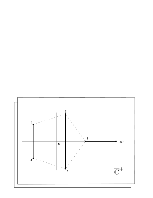
Figure 1: The two sheets $\bar{\mathbb{C}}^{\pm}$ of $\Gamma_{5}$ with the branch points and cuts (solid lines).

The passage from one $\bar{\mathbb{C}}$-sheet to the other is realized through any of the three cuts that join the pairs $(Q_{2},Q_{5})$, $(Q_{3},Q_{4})$ and $(Q_{1},\infty)$ on $\bar{\mathbb{C}}^{+}$ and $\bar{\mathbb{C}}^{-}$ and that do not intersect each other. Let us fix a canonical basis of cycles $a_{1},a_{2},b_{1},b_{2}$ on $\Gamma$ such that

$${a}_{i}\circ{a}_{j}={b}_{i}\circ{b}_{j}=0,\quad a_{i}\circ b_{j}=\delta_{ij},\qquad i,j=1,2,$$

where $\gamma_{1}\circ\gamma_{2}$ denotes the intersection index of the cycles $\gamma_{1},\gamma_{2}$. Following the common convention, $a$-cycles lie entirely on the upper sheet $\bar{\mathbb{C}}^{+}$ and embrace one of the cuts while $b$-cycles run through both sheets. We assume that $a_{1}$ embraces $(Q_{1},\infty)$ and $b_{1}$ joins $\infty$ with $Q_{3}$, so that the projections of cycles $a_{1},b_{1}$ embrace $\infty$. For the pentagonal curve $\Gamma_{5}=\{(\eta,\mu)|\,\mu^{2}=\eta^{5}-E\}$, the $\eta$-coordinates of the finite branch points are

$$\eta_{b}^{(k)}=\exp\left(\frac{2\pi{\rm i}(k-1)}{5}+\frac{1}{5}\arg E\right)\sqrt[5]{|E|},\quad k=1,\dots,5.$$

For real $E>0$, the branch points and cuts are depicted in Figure 1, where $\bar{\mathbb{C}}^{\pm}$ are shown as planes and $Q_{j}$ are denoted just by their indices $j$. Figure 2 also shows the canonical cycles, where segments of the cycles $b_{1},b_{2}$ on the upper and lower sheets are given by solid and dashed lines respectively. Since the branch points $(Q_{i},0)$, $i=1,\dots,5$ are just the five complex roots $E^{1/5}$, for generic (complex) values of $E$ their position is simply obtained by a rotation and scaling of the pentagon of Figure 2.

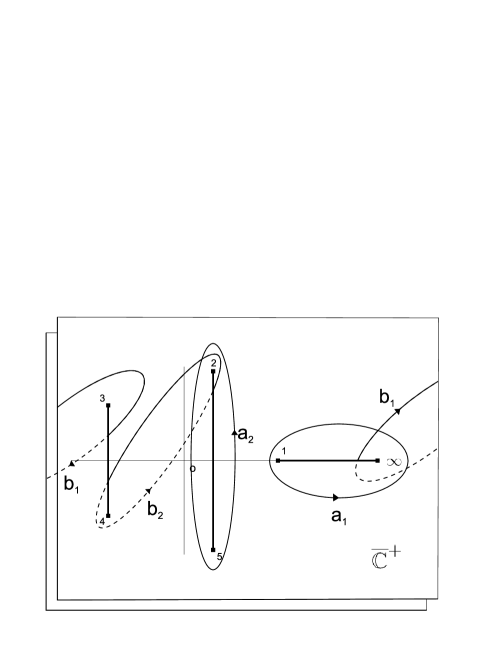
Figure 2: Canonical cycles $a_{i}$ and $b_{i}$, $i=1,2$ for the pentagonal curve $\Gamma_{5}=\{(\eta,\mu)|\,\mu^{2}=\eta^{5}-E\}$. Segments of cycles on the upper and lower sheet are depicted as solid and dashed lines respectively.

We introduce next the following basis of holomorphic differentials $\left(\frac{d\eta}{\mu},\frac{\eta\,d\eta}{\mu}\right)$ on $\Gamma$ and consider in detail the problem of inverting the hyperelliptic integral

$$\tau=\int_{\infty}^{P}\frac{d\eta}{\sqrt{2}\,\mu},\qquad P=(\eta,\mu)\in\Gamma.$$ (17)

The integral has four independent complex periods defined by:

$$V_{1}=\oint_{a_{1}}\frac{d\eta}{\sqrt{2}\,\mu},\quad V_{2}=\oint_{a_{2}}\frac{d\eta}{\sqrt{2}\,\mu},\quad V_{3}=\oint_{b_{1}}\frac{d\eta}{\sqrt{2}\,\mu},\quad V_{4}=\oint_{b_{2}}\frac{d\eta}{\sqrt{2}\,\mu}.$$ (18)

It follows that the inverse complex functions $\eta(\tau)$, $\mu(\tau)$ should have four generally independent periods on $\mathbb{C}$. This is not possible, a fact that was already noted by Jacobi (see [27] for an historical account). If the periods $V_{1},\dots,V_{4}$ are not commensurable, then the functions $\eta(\tau)$, $\mu(\tau)$ cannot be singled valued on ${\mathbb{C}}=\{\tau\}$, but they can be regarded as single-valued on an infinitely sheeted covering ${\mathcal{R}}\mapsto{\mathbb{C}}$. This Riemann surface has an infinite number of ramification points whose projections onto the $\tau$-plane form a dense set.

Remark 1

According to the Weierstrass–Poincaré theory of reductions of Abelian functions, (see e.g. the surveys [5, 6]), the periods of ${d\eta}/\mu$ may become commensurable in special cases when the genus 2 curve $\Gamma$ covers an elliptic curve $\mathcal{E}$ and the differential $d\eta/\mu$ is a pull-back of a holomorphic differential on $\mathcal{E}$. Then ${\mathcal{R}}\mapsto{\mathbb{C}}$ is just a finite order covering. For genus 2 curves admitting a finite order automorphism, a complete list of their Riemann matrices that characterize such coverings was given by Bolza in [9] (see also [8]).

We note that the pentagonal curve $\Gamma_{5}=\{\mu^{2}=E-\eta^{5}\}$ does not belong to this list, hence its periods are incommensurable (see also Proposition 7 and relation (22) below). On the contrary, the sextic curve $\Gamma_{6}=\{\mu^{2}=E-\eta^{6}\}$ does appear in Bolza’s list: it is a 2-fold ramified cover of two elliptic curves,

$$\begin{CD}{\mathcal{E}}_{1}@ <\pi_{1}<<\Gamma_{6}@ >\pi_{2}>>{\mathcal{E}}_{2},\end{CD}$$

$${\mathcal{E}}_{1}=\{w_{1}^{2}=E-z_{1}^{3}\},\quad{\mathcal{E}}_{2}=\{w_{2}^{2}=z_{2}(E-z_{2}^{3})\},$$

$$(z_{1},w_{1})=\pi_{1}(\eta,\mu)=(\eta^{2},\mu),\quad(z_{2},w_{2})=\pi_{2}(\eta,\mu)=(\eta^{2},\eta\mu).$$

Then $d\eta/\mu$ is the pullback of the holomorphic differential $dz_{2}/w_{2}$ on ${\mathcal{E}}_{2}$. As a result, the corresponding covering ${\mathcal{R}}\mapsto{\mathbb{C}}$ is only 2-fold, which implies that, similarly to the case of the system (11), all the solutions of equations (14) are periodic, either with period $T=2\pi/\omega$ or $2T$.

Remark 2

Note that for an arbitrary curve $\Gamma$ given by (16), the differential $d\eta/\mu$ has a double zero at $\infty$ and no zeros elsewhere. Namely, choosing a local coordinate $\delta(P)$ in a neighborhood of $\infty\in\Gamma$ such that $\delta(\infty)=0$ and $\eta=1/\delta^{2}$, $\mu=O(1/\delta^{5})$, one has $d\eta/\mu=O(\delta^{2})\,d\delta$ and, therefore, $\tau=O(\delta^{3})$, $\delta=O\left(\sqrt[3]{\tau}\right)$. This implies that the functions $\eta(\tau),\mu(\tau)$ have only critical points $\tau_{*}$ with the behavior

$$\begin{gathered}\eta(\tau)=(\tau-\tau_{*})^{-2/3}(c_{0}+c_{1}(\tau-\tau_{*})^{2/3}+c_{2}(\tau-\tau_{*})^{4/3}+\cdots),\\ \mu(\tau)=(\tau-\tau_{*})^{-5/3}(d_{0}+d_{1}(\tau-\tau_{*})^{2/3}+d_{2}(\tau-\tau_{*})^{4/3}+\cdots),\end{gathered}$$ (19)

where $c_{j}$ and $d_{j}$ are constants. Thus, the singularities $\tau_{*}$ are $3^{\footnotesize\mbox{rd}}$ order branch points of the covering ${\mathcal{R}}\mapsto{\mathbb{C}}$ and there is no other type of branching.

Despite the complexity of the Riemann surface $\mathcal{R}$, it is possible to give an explicit description of its geometric and topological structure, which enables us to describe the behavior of the solutions of system (12). Such an explicit description of $\mathcal{R}$ is new to our best knowledge.

Description of a sheet of $\mathcal{R}$

We start by making some preliminary observations. Namely, on the $\bar{\mathbb{C}}^{+}$–sheet of $\Gamma$ we make two extra cuts $B_{1}^{+}$ and $B_{2}^{+}$ that join $\infty$ with $Q_{1}$ and $Q_{3}$, respectively (see Figure 3). We assume that $B_{1}^{+}$ and $B_{2}^{+}$ are embraced by projections of the cycles $a_{1}$ and $b_{1}$. It is always possible to choose the cuts in such a way that path integral (17) along each of them yields a straight line segment on the complex $\tau$-plane. We also introduce the two cuts $B_{1}^{-}$ and $B_{2}^{-}$ on the $\bar{\mathbb{C}}^{-}$–sheet with the same properties (in Figure 3 such cuts are depicted as the bold dotted lines.)

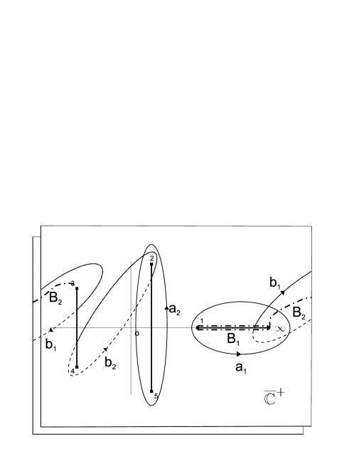
Figure 3: Canonical cycles $a_{i}$ and $b_{i}$ and the new cuts $B_{1}$ and $B_{2}$ (dashed-dotted lines) needed to define the B-rule.

Definition 3 (B-rule)

Consider the hyperelliptic integral (17) and allow the point $P$ to range over the whole curve $\Gamma$ in such a way that the integration path from $\infty$ to $P$ does not cross any of the cuts $B_{1}^{\pm}$ and $B_{2}^{\pm}$. We shall refer to this condition as the Border rule, or for simplicity, the $B$-rule.

Note that since the cycles $a_{1}$ and $b_{1}$ cross the cuts $B_{2}$ and $B_{1}$ respectively, the corresponding periods $V_{1}$ and $V_{3}$ are not allowed by the $B$-rule, and we shall refer to them as the forbidden periods. Consequently, we shall refer to the other periods $V_{2}$ and $V_{4}$ as the allowed periods.

Proposition 4

Under the B-rule, the values of the integral $\tau(P)$ range over the whole complex plane $\mathbb{C}$ except for an infinite number of non-intersecting identical domains $W_{ij}$, $i,j\in{\mathbb{Z}}$ which shall be called windows. Each window is a parallelogram spanned by the forbidden periods $V_{1}$ and $V_{3}$, while the window lattice $W_{ij}$ is generated by the allowed periods $V_{2}$ and $V_{4}$. The corners of the windows correspond to the image of the point at $\infty\in\Gamma$. At each pair of points $\tau_{1},\tau_{2}$ lying on the opposite edges of $W_{ij}$ such that $\tau_{2}=\tau_{1}+V_{1}$ or $\tau_{2}=\tau_{1}+V_{3}$ the coordinates $\eta,\mu$ take the same values.

In other words, the window $W_{i,j+1}$ ($W_{i+1,j}$ ) is obtained from $W_{i,j}$ shifting by period $V_{2}$ ($V_{4}$). When $P\in\Gamma$ makes a linear combination of cycles $a_{2},b_{2}$, the image $\tau(P)$ shifts by the corresponding combination of $V_{2},V_{4}$. More specifically, the two edges of the windows parallel to $V_{1}$ ($V_{3}$) are the image of the two opposite sides of the cut $B_{1}^{\pm}$ ($B_{2}^{\pm}$).

It follows that under the border rule, the two inverse functions $\eta(\tau)$ and $\mu(\tau)$ are quasi-elliptic, in the sense that they are doubly periodic with the allowed periods $V_{2}$ and $V_{4}$, but they are not defined in the whole complex $\tau$-plane. The domain of definition ${\mathcal{D}}={\mathbb{C}}\setminus\{\cup\;W_{ij}\}$ can be regarded as one of the infinite set of sheets of the Riemann surface $\mathcal{R}$. Inside each parallelogram of periods $V_{2}$ and $V_{4}$ the functions have 4 poles lying at the corners of a window $W_{ij}$. This is the equivalent of a fundamental domain for the “quasi-elliptic” functions $\eta(\tau)$ and $\mu(\tau)$under the B-rule. For a general genus 2 curve $\Gamma$ with two real periods, the domain ${\mathcal{D}}$ is depicted in Figure 4 as the grey shaded area.

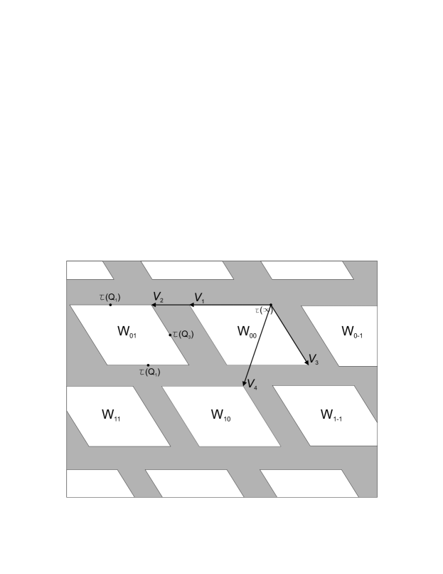
Figure 4: Domain $\mathcal{D}$ (shaded area) and windows $W_{ij}$. We can consider this to be one of the infinite number of sheets of the Riemann surface $\mathcal{R}$

Proof of Proposition 4. Let us first study the integral $\tau(P)$ when $P\in\Gamma$ moves along the cuts $B_{1}^{\pm}$ and $B_{2}^{\pm}$ without crossing them. When $P$ moves on $\bar{\mathbb{C}}^{+}$ from $\infty$ to $Q_{1}$ along the upper edge of $B_{1}^{+}$ and returns to $\infty$ along the lower edge of $B_{1}^{+}$, the point $\tau(P)$ performs a straight line motion along the forbidden period vector $V_{1}$. If $P$ continues moving on $\bar{\mathbb{C}}^{+}$ from $\infty$ to $Q_{1}$ along the lower edge of $B_{2}^{+}$ and returns to $\infty$ along the upper edge of $B_{2}^{-}$ on $\bar{\mathbb{C}}^{-}$, the integral $\tau(P)$ traces the second forbidden period vector $V_{3}$. If $P$ traces the same two motions now on the opposite $\bar{\mathbb{C}}$-sheets of $\Gamma$, the point $\tau(P)$ moves subsequently along the vectors $-V_{1}$ and $-V_{3}$. Corresponding to this sequence of motions of $\tau$ along the cuts the integral $\tau(P)$ traces a parallelogram $W$ spanned by the forbidden periods on the $\tau$-plane. The coordinates $\eta,\mu$ of $P$ coincide along the points on the upper edge of $B_{1}^{+}$ ($B_{1}^{-}$) identified with the the lower edge of $B_{1}^{-}$ ($B_{1}^{+}$), and they also coincide along the opposite points on the upper and lower edges of $B_{2}^{+}$ ($B_{2}^{-}$). Under the B-rule the point $\tau(P)$ cannot reach inside of a window $W$. Outside of $W$, $\tau(P)$ behaves as an elliptic integral of the first kind with periods $V_{2}$ and $V_{4}$, therefore $\tau(P)$ cannot reach inside of an infinite number of windows $W_{ij}$ obtained from $W$ by translations by the allowed periods. Since the map $\tau(P)$ is analytical, in ${\mathbb{C}}=\{\tau\}$ each $W_{ij}$ has a small neighborhood covered by the image of $P$, hence the parallelograms cannot intersect. Finally, the proof that $\tau(P)$ reaches any point of ${\mathcal{D}}={\mathbb{C}}\setminus\{\cup\;W_{ij}\}$ goes along the same lines as that for any elliptic integral of the first kind. $\square$

3.1 Gluing the ${\mathcal{D}}$-sheets together.

Let us first introduce some notation for the different edges of a window $W_{ij}$ on $\mathcal{D}$: we shall label them as $N$ (“North”), $W$ (“West”), $S$ (“South”), and $E$ (“East”). By convention, the $N$- and $S$-edges are spanned by the period $V_{1}$, while the $W$- and $E$-edges lie along $V_{3}$. Next, we assume that the $B$-rule can be violated and we allow the integration path from $\infty$ to $P$ to cross one of the cuts $B_{1}^{\pm},B_{2}^{\pm}$ only once. If the path crosses $B_{1}^{-},\;(B_{1}^{+})$, then the point leaves the domain $\mathcal{D}$ through $S$-edge (respectively, $N$-edge) of a window $W_{ij}$.

In view of Proposition 4, this motion can be viewed as the passage to a different sheet ${\mathcal{D}}^{\prime}$ of the surface $\mathcal{R}$, which is a translate of an identical copy of $\mathcal{D}$ and has the same window lattice structure. On crossing the $S$-edge of $W_{ij}$ on $\mathcal{D}$, the image $\tau(P)$ immediately arrives at the $N$-edge of a window $W_{ij}^{\prime}$ of ${\mathcal{D}}^{\prime}$ and then continues travelling on this new sheet. That is, the $N$-edge of a window $W_{ij}^{\prime}$ on ${\mathcal{D}}^{\prime}$ is glued to the $S$-edge of $W_{ij}$ on ${\mathcal{D}}$ in such a way that the corners are connected to corners and at the identified points the values of $\eta,\mu$ coincide. Next, on crossing the $N$-edge of the window $W_{ij}$ on $\mathcal{D}$, $\tau(P)$ enters another sheet $\mathcal{D}^{\prime\prime}$ from the $S$-edge of a window $W_{ij}^{\prime\prime}$ on $\mathcal{D}^{\prime\prime}$ . Similarly, when the integration path on $\Gamma$ crosses $B_{2}^{-},\;(B_{2}^{+})$, then $\tau(P)$ leaves $\mathcal{D}$ through the $E$- (respectively, $W$-) edge of the window $W_{ij}$ and arrives at other sheets of $\mathcal{R}$ from the $W$- (respectively, $E$-) edges of windows on these new sheets.

Since there is an infinite number of windows on $\mathcal{D}$, one might think that each sheet is connected to an infinite set of different $\mathcal{D}$-sheets of $\mathcal{R}$. However, the actual structure of $\mathcal{R}$ is simpler and completely described by the following short proposition.

Proposition 5

The Riemann surface $\mathcal{R}$ is a union of an infinite number of identical $\mathcal{D}$-sheets glued to each other along the corresponding opposite edges of their windows. Any arbitrarily chosen “home” sheet ${\mathcal{D}}_{H}$ is connected to precisely four other sheets ${\mathcal{D}}_{HN},{\mathcal{D}}_{HE},{\mathcal{D}}_{HS},{\mathcal{D}}_{HW}$ and the passage from ${\mathcal{D}}_{H}$ to them is realized by crossing respectively the $S$-, $W$-, $N$-, and, $E$-edge of any window $W_{ij}$ on ${\mathcal{D}}_{H}$.

Proof of Proposition. We only need to prove that passage through $S-$ (or $W$- or $N$- or $E$-) edges of different windows of ${\mathcal{D}}_{H}$ leads to the same ${\mathcal{D}}$-sheet of ${\mathcal{R}}$.

Let $p(t)$ be a path on $\Gamma$ that starts at a point $P_{0}$, crosses the border $B_{1}^{\pm}\cup B_{2}^{\pm}$ once and ends at a point $P_{1}$. Next, let $p^{(1)}(t)$ be the path $p(t)$ followed by a linear combination of cycles $a_{2},b_{2}$ and $p^{(2)}(t)$ be the same linear combination of cycles (with starting point $P_{0}$) followed by the path $p(t)$. Then the integrals $\tau(p^{(1)}(t))$, $\tau(p^{(2)}(t))$ give paths $\gamma_{1},\gamma_{2}$ on ${\mathcal{R}}$ that start at the same point on the sheet ${\mathcal{D}}_{H}$ and leave it through the same edges of different windows on ${\mathcal{D}}_{H}$. By construction of $p^{(1)}(t)$ and $p^{(2)}(t)$, the endpoints of cycles $\gamma_{1}$ and $\gamma_{2}$ have the same $\tau$-coordinate, as well as the same $\eta,\mu$-coordinates (corresponding to $P_{1}\in\Gamma$). Hence, the endpoints on ${\mathcal{R}}$ coincide, and by continuity the corresponding ${\mathcal{D}}$-sheets can be identified. $\square$

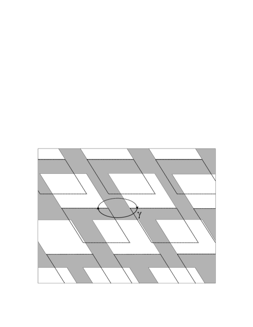
Figure 5: Window lattice on $\mathcal{D}_{H}$ (bold) and on $\mathcal{D}_{HN}$ (dotted). The path leaves $\mathcal{D}_{H}$ through the $S$-side of a window (bold arc) and enters $\mathcal{D}_{HN}$ , then it continues on $\mathcal{D}_{HN}$ (dotted arc) and leaves the sheet through the $N$-edge of a window, coming back to $\mathcal{D}_{H}$

As a corollary of the above proposition, we note that each of the four $\mathcal{D}$-sheets adjacent to ${\mathcal{D}}_{H}$ is in turn connected in the same way to other four sheets, one of them being the initial sheet ${\mathcal{D}}_{H}$. In particular, when $\tau(P)$ leaves ${\mathcal{D}}_{H}$ through the $S$-edge of a window $W_{ij}$, enters the sheet ${\mathcal{D}}_{H,N}$ and then leaves it through the $N$-edge of another window $W^{\prime}_{ij}$ in ${\mathcal{D}}_{H,N}$, then it returns to ${\mathcal{D}}_{H}$ (see the illustration in Figure 5). It is then natural to label the ${\mathcal{D}}$-sheets connected to ${\mathcal{D}}_{HN}$ as ${\mathcal{D}}_{HNN}$, ${\mathcal{D}}_{HNE}$, ${\mathcal{D}}_{HNW}$, and ${\mathcal{D}}_{HNS}={\mathcal{D}}_{H}$.

Finally, we also state the important

Lemma 6

The passages between $\mathcal{D}$-sheets in the “horizontal” ($E$, $W$)-direction and the “vertical” ($N$, $S$)-direction commute. That is, the following sheets coincide:

$${\mathcal{D}}_{HNE}={\mathcal{D}}_{HEN},\quad{\mathcal{D}}_{HNW}={\mathcal{D}}_{HWN},\quad{\mathcal{D}}_{HSE}={\mathcal{D}}_{HES},\quad{\mathcal{D}}_{HSW}={\mathcal{D}}_{HWS}.$$

Proof of Lemma. Indeed, the windows on ${\mathcal{D}}_{HNE}$ and on ${\mathcal{D}}_{HEN}$ are obtained from those on ${\mathcal{D}}_{H}$ by shift by the same vector $V_{1}-V_{3}$, hence ${\mathcal{D}}_{HNE}$ and ${\mathcal{D}}_{HEN}$ can be identified. Similar arguments apply to identify the other pairs of sheets. $\square$

As a result, the Riemann surface $\mathcal{R}$ can be described as a ${\mathbb{Z}}^{2}$-countable set of $\mathcal{D}$-sheets, that is

$${\mathcal{R}}=\{\cup\,{\mathcal{D}}_{ij}\mid i,j\in{\mathbb{Z}}\}$$

where $i,j$ enumerate the passages in the “horizontal” and “vertical” directions respectively. Hence, travelling on $\mathcal{R}$ can be encoded as a path (sequence) on a ${\mathbb{Z}}^{2}$-lattice $\Lambda$.

3.2 Branching of the projection $\mathcal{R}\mapsto\mathbb{C}=\{\tau\}$.

Note that each corner of a window on a $\mathcal{D}$-sheet is connected to several different sheets, hence the corners are branch points of the projection $\Pi\,:\,{\mathcal{R}}\mapsto{\mathbb{C}}=\{\tau\}$. In particular, consider the corner $\tau_{*}$ between the $E$- and $S$-edges of $W_{ij}$ on ${\mathcal{D}}_{H}$. Let $\gamma_{*}$ be a path on $\mathcal{R}$ that starts on ${\mathcal{D}}_{H}$ and whose projection to $\{\tau\}$ is a sufficiently small circle around $\tau_{*}$ with a counter-clockwise orientation. Then $\gamma_{*}$ leaves ${\mathcal{D}}_{H}$ through the $S$-side of a window and visits the sequence of sheets

$${\mathcal{D}}_{H}\to{\mathcal{D}}_{HN}\to{\mathcal{D}}_{HNE}(={\mathcal{D}}_{HEN})\to{\mathcal{D}}_{HE}\to{\mathcal{D}}_{H}.$$

Thus $\tau_{*}$ connects four $\mathcal{D}$-sheets and four edges of windows on them, and the path $\gamma_{*}$ closes after making 3 complete rotations about $\tau_{*}$. This gives a geometric interpretation of the cubic root branching of functions $\eta(\tau)$ and $\mu(\tau)$ in (19). The other window corners have the same properties. Note that there is no contradiction between the fact that each branchpoint $\tau_{*}$ is of the third order but connects four $\mathcal{D}$-sheets together. The reason is that the $\mathcal{D}$-sheets are not copies of the whole complex plane $\mathbb{C}$, and due to the presence of the windows it is not possible to turn by $2\pi$ around $\tau_{*}$ on a $\mathcal{D}$-sheet.

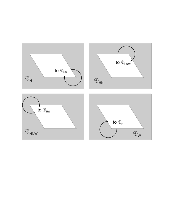
Figure 6: A closed path on $\mathcal{R}$ around cubic branch point.

Due to the incommensurability of the size of the windows (the modulus of the forbidden periods $|V_{1}|$ and $|V_{3}$) with the shift vectors that generate the windows lattice (the allowed periods $V_{2}$ and $V_{4}$), the projection of the corners of all the windows in all the sheets of $\mathcal{R}$ (i.e., the branch points of $\Pi$) is a dense set in $\mathbb{C}$. However, as we have seen above, on each of the infinite ${\mathcal{D}}$-sheets of $\mathcal{R}$ the branch points are isolated and they form a regular lattice.

3.3 Duality.

The ${\mathbb{Z}}^{2}$-lattice $\Lambda$ introduced above has a much richer structure. More precisely, one can extend it to a cell structure $\bar{\Lambda}$ on ${\mathbb{R}}^{2}$: the adjacent vertices of the lattice are regarded as vertices of square cells $\Delta_{kl}$ on ${\mathbb{R}}^{2}$.

There is a remarkable duality between the objects of ${\mathcal{R}}$ and $\bar{\Lambda}$: a 2-dimensional $\mathcal{D}$-sheet in $\mathcal{R}$ corresponds to a vertex of $\Lambda$, the edges of the windows connecting two different $\mathcal{D}$-sheets of ${\mathcal{R}}$ correspond to the segments joining the two corresponding vertices. Finally, a branchpoint $\tau^{*}$ of ${\mathcal{R}}$ which connects four $\mathcal{D}$-sheets corresponds to the square cell $\Delta_{kl}$ in $\bar{\Lambda}$ defined by the four vertices which correspond to the sheets.

3.4 The surface $\mathcal{R}$ as the universal covering of the theta-divisor.

Now, instead of the single hyperelliptic integral (17), consider the vector of holomorphic integrals

$$(u_{1},u_{2})^{T}=\int_{\infty}^{P}\left(\frac{d\eta}{\mu},\frac{\eta\,d\eta}{\mu}\right)^{T},\qquad P\in\Gamma,$$

which has 4 independent vectors of periods in ${\mathbb{C}}^{2}(u_{1},u_{2})$ with respect to the cycles $a_{1},\dots,b_{2}$. As it is known from the theory of Abelian varieties, the map ${\mathcal{A}}\,:\,P\mapsto(u_{1},u_{2})^{T}$ describes a well defined smooth embedding of $\Gamma$ into the Jacobian variety Jac$(\Gamma)={\mathbb{C}}^{2}/\Lambda$, where $\Lambda$ is the lattice generated by the above period vectors. The image of the embedding is known to be a one-dimensional analytic subvariety $\Theta^{\prime}\subset$ Jac$(\Gamma)$, a translate of the theta-divisor defined as the zero locus of the Riemann theta-function $\theta(u_{1},u_{2})$ of the curve $\Gamma$.

Let $\widetilde{\Theta}\subset{\mathbb{C}}^{2}$ be the universal covering of $\Theta$. Note that it can also be regarded as an infinitely sheeted ramified covering of ${\mathbb{C}}=\{u_{1}\}$ and that the first coordinate $u_{1}$ jointly with the point $P\in\Gamma$ define a point of $\widetilde{\Theta}$ uniquely. It follows that by identifying $u_{1}$ with the complex coordinate $\tau$ in (17), one can also identify the universal covering $\widetilde{\Theta}$ with our Riemann surface $\mathcal{R}$: two points on both complex surfaces are identified if and only if they are projected to the same $u_{1}=\tau$ and correspond to the same point on $\Gamma$.

3.5 Periods of the pentagonal curve.

The existence of a group of automorphisms of the curve $\Gamma_{5}=\{\mu^{2}=E-\eta^{5}\}$ implies some special relations between its periods, which we did not find in the literature and indicate here.

Proposition 7

For the chosen basis of cycles on $\Gamma_{5}$, the local dependence of the periods on the complex energy is as follows

$$V_{i}(E)=E^{-3/10}V_{i}^{0},\qquad i=1,\dots,4,$$ (20)

where $V_{i}^{0}$ are the periods for $E=1$ given by

$$V_{1}^{0} =2\int_{\infty}^{1}\frac{d\eta}{\sqrt{1-\eta^{5}}}\,\cong\,1.819915\,{\rm i}$$ (21)

$$V_{2}^{0} =-\frac{3+\sqrt{5}}{2}\,V_{1}^{0},$$

$$V_{3}^{0} =-{\rm e}^{-{\rm i}\pi/5}V_{1}^{0},$$

$$V_{4}^{0} =-\frac{3+\sqrt{5}}{2}\,V_{3}^{0},$$

Note that when $E$ varies along a loop embracing the origin and returns to its original value, the curve $\Gamma_{5}$ undergoes the automorphism $\rho$ that rotates its finite branch points by angle $2\pi/5$, whereas the periods undergo a monodromy: they are all multiplied by $\exp(-3\pi i/5)$ and, on the other hand, become linear combinations of $V_{1}^{0},\cdots,V_{4}^{0}$ with integer coefficients. Proposition (21) implies that for any complex energy $E$ the following relations hold

$$\frac{V_{2}}{V_{1}}=\frac{V_{4}}{V_{3}}=-\frac{3+\sqrt{5}}{2}\,,\quad|V_{1}|=|V_{3}|,\quad|V_{2}|=|V_{4}|.$$ (22)

The two forbidden (allowed) periods have the same length, moreover the forbidden period $V_{1}$ ($V_{3}$) on $\mathbb{C}$ is proportional to the allowed period $V_{2}$ ($V_{4}$). Since the proportionality constant is an irrational number, the period vectors are not commensurable, as was also claimed in Remark 2.1.

It is worth noting that the pentagonal curve $\Gamma_{5}$ is rather special, and the form of the windows on ${\mathcal{D}}$ for a generic genus 2 curve $\{\mu^{2}=P_{5}(\eta)-E\}$ depends on $E$ in a nontrivial way: $V_{i}$ form a fundamental basis of solutions of a fourth order Picard–Fuchs ODE with the independent variable $E$. A sketch of the proof of Proposition 7 Under the subsitution $\eta=E^{1/5}\lambda$, the holomorphic differential $d\eta/\mu$ takes the form $E^{-3/10}\,d\lambda/\sqrt{1-\lambda^{5}}$, while on the $\lambda$-plane the branch points and the integration cycles are the same as on $\eta$-plane for $E=1$. This implies the relations (20). The calculation of the periods $V_{1}^{0},\cdots,V_{4}^{0}$ follow the ideas of [9]. More specifically, the monodromy transformation described above implies that the periods $V_{i}^{0}$ must satisfy a system of homogeneous linear equations with integer coefficients

$$\exp(-3\pi i/5)V_{i}^{0}=\alpha_{i1}V_{1}+\cdots+\alpha_{i4}V_{4},\qquad\alpha_{ik}\in{\mathbb{Z}}.$$

Expressing the deformed cycles $\rho(a_{1}),\dots,\rho(b_{2})$ in terms of the original cycles on $\Gamma_{5}$ for $E=1$, it is possible to calculate the coefficients $\alpha_{ik}$. Finally, solving this system and numerical integration of $V_{1}^{0}$ yields expressions (21). $\square$

4 Circular Travelling on the Surface $\mathcal{R}$

As mentioned in Section 1, one can consider a complex solution of the system (1.12) with $t\in{\mathbb{R}}$ as a smooth path $\gamma(t)$ on the infinitely sheeted surface $\mathcal{R}$ corresponding to the curve $\Gamma$ such that the projection $\Pi(\gamma(t))$ is the circle $\mathcal{C}$ on the $\tau$-plane parameterized by (4) and thus having radius $1/\omega$.

4.1 A geometrical algorithm

Comparing the quadrature (13) and the integral (17), we find that for initial complex conditions $\zeta_{0},\zeta^{\prime}_{0}$, the $\tau$-coordinate of the starting point $\gamma_{0}=\gamma(0)$ is

$$\tau_{0}=\int_{\infty}^{\zeta_{0}}\frac{d\eta}{\sqrt{2}\sqrt{E-\eta^{5}}},$$ (23)

where the energy $E$ is defined in (1) and the sign of the root is chosen in accordance with the sign of $\zeta^{\prime}(0)$.

Geometrically, $\gamma_{0}$ can be chosen on any ${\mathcal{D}}$-sheet by adding $\tau_{0}$ to a corner of any window. By convention, the chosen initial sheet is labelled as ${\mathcal{D}}_{00}$.

Let ${\mathcal{C}}_{0}$ be the preimage of the circle ${\mathcal{C}}$ on ${\mathcal{D}}_{00}$. Naturally, if ${\mathcal{C}}_{0}$ does not cross any window on ${\mathcal{D}}_{00}$, then the path $\Pi^{-1}\,{\mathcal{C}}$ on $\mathcal{R}$ remains on ${\mathcal{D}}_{00}$ and the solution $\zeta(t)$ of (9) is periodic with the fundamental period $T=2\pi/\omega$. In other cases the path $\gamma(t)$ gives rise to a finite or infinite sequence on the ${\mathbb{Z}}^{2}$-lattice $\{\cup\,{\mathcal{D}}_{ij}\mid i,j\in{\mathbb{Z}}\}$ according to the following algorithm:

1) Given position of the circle ${\mathcal{C}}_{0}$ on ${\mathcal{D}}_{00}$ with the initial point $\gamma_{0}\in{\mathcal{C}}_{0}$, one determines the points of its intersection with the edges of ${\mathcal{W}}_{ij}$. Among them one chooses the point $\gamma_{1}$, which is closest to $\gamma_{0}$ in the counterclockwise direction on ${\mathcal{C}}_{0}$.

2) Given $\gamma_{1}$ and the edge containing it, one finds the point $\gamma_{1}^{\prime}$ on the opposite edge of the same window such that

$$\gamma_{1}^{\prime}=\gamma_{1}\pm V_{1}\quad\mbox{or }\quad\gamma_{1}^{\prime}=\gamma_{1}\pm V_{3}.$$

Then $\gamma(t)$ passes to the new sheet ${\mathcal{D}}^{\prime}={\mathcal{D}}_{0,\pm 1}$ (respectively, ${\mathcal{D}}^{\prime}={\mathcal{D}}_{\pm 1,0}$) with $\gamma_{1}^{\prime}$ as the starting point on ${\mathcal{D}}^{\prime}$.

3) On the new sheet ${\mathcal{D}}^{\prime}$ one constructs the circle ${\mathcal{C}}_{1}$ by translating ${\mathcal{C}}_{0}$ by $\pm V_{1}$ (respectively $\pm V_{3}$) so that $\gamma_{1}^{\prime}\in{\mathcal{C}}_{1}$. One then determines the intersections of ${\mathcal{C}}_{1}$ with edges of windows on ${\mathcal{D}}^{\prime}$ and chooses the intersection point $\gamma_{2}$, which is closest to $\gamma_{1}^{\prime}$ in the clockwise direction on ${\mathcal{C}}_{1}$.

Then the procedure repeats as in step 2) with ${\mathcal{D}}_{00}$ and $\gamma_{1}$ replaced by ${\mathcal{D}}^{\prime}$ and $\gamma_{2}$.

4) If after $n$ iterations one returns to ${\mathcal{D}}_{00}$, then the corresponding circle ${\mathcal{C}}_{n-1}$ necessarily coincides with ${\mathcal{C}}_{0}$. If the segment of ${\mathcal{C}}_{0}$ between $\gamma_{n}$ and $\gamma_{n+1}$ contains $\gamma_{0}$, then the procedure stops and $\gamma(t)$ is closed. Otherwise, the algorithm continues on step 1) with $\gamma_{0}$ replaced by $\gamma_{n}$.

This geometric algorithm for travelling on the fundamental domain includes the essential properties of the flow defined by the system (12) and allows to predict the period of the orbit without numerical integration.

4.2 Motion on a fundamental domain $\tilde{\mathcal{D}}$.

There is an equivalent description of the procedure. Namely, let $\hat{\mathcal{D}}$ be a fundamental parallelogram of allowed periods $V_{2}$ and $V_{4}$ on $\mathcal{D}$ that contains a window ${\mathcal{W}}^{*}$ completely inside. Then $\hat{\mathcal{D}}$ does not have any other windows inside and there is a natural bijection between the fundamental domain $\tilde{\mathcal{D}}=\hat{\mathcal{D}}\setminus{\mathcal{W}}^{*}\subset{\mathcal{D}}$ and the curve $\Gamma$. A smooth path $\gamma(t)=\Pi^{-1}\,{\mathcal{C}}$ on $\mathcal{R}$ induces a smooth path $P(t)$ on $\Gamma$ and a generally discontinuous path $\tilde{\gamma}(t)$ on $\tilde{\mathcal{D}}$ that consists of segments of translates of ${\mathcal{C}}_{0}$: when $\tilde{\gamma}(t)$ crosses an exterior edge of $\tilde{\mathcal{D}}$ at a point $\gamma^{*}$, it reappears on the point $\gamma^{**}$ on the opposite exterior edge of the domain, since both points correspond to the same point on $\Gamma$. Similarly, on crossing an edge of the interior window of $\tilde{\mathcal{D}}$, the trajectory continues from the opposite edge of the window as described in step 2) of the algorithm. Example For the pentagonal curve with the complex energy $E=1110+i\,1452$, a fragment of the initial sheet ${\mathcal{D}}_{00}$ and the corresponding fundamental domain $\tilde{\mathcal{D}}$ are presented in Figure 7a), and 7b) respectively. Here we also show an example of the circle ${\mathcal{C}}_{0}$ on ${\mathcal{D}}_{00}$, which generates a periodic path $\tilde{\gamma}(t)$ in $\tilde{\mathcal{D}}$ with period $7T$. The corresponding periodic sequence on the ${\mathbb{Z}}^{2}$-lattice is

$$\overline{(0,0)} \to(-1,0)\to(0,0)\to\overline{(-1,0)}\to(-1,1)\to\overline{(0,1)}\to(0,2)\to$$

$$\overline{(1,2)} \to(1,1)\to(1,2)\to(1,1)\to\overline{(2,1)}\to(1,1)\to(2,1)\to$$

$$(2,0) \to\overline{(1,0)}\to(1,-1)\to\overline{(0,-1)}\to(0,0)\to(0,-1)\to\overline{(0,0)}.$$

where the bars mark the ${\mathcal{D}}$-sheets visited when the projection $\Pi\gamma(t)$ performs a complete turn. Applying the above algorithm to different initial conditions, we obtained a great variety of periodic trajectories. In all cases we observed a perfect coincidence of the motion in $\tilde{\mathcal{D}}$ with the results obtained by the numeric integration of the equations (9) and (12).

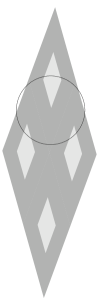
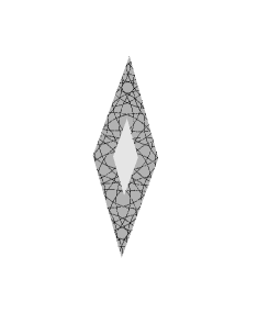
(a)	(b)
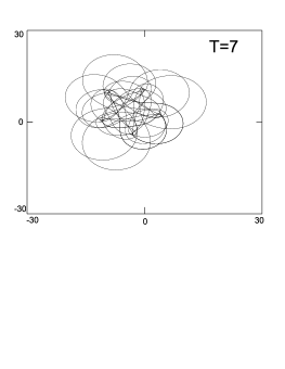
(c)	(d)

Figure 7: (a) Circle $\mathcal{C}_{0}$ on the initial sheet $\mathcal{D}_{00}$. (b) Path $\tilde{\gamma}(t)$ on the fundamental domain $\tilde{D}$. (c) Sequence of sheets of $\mathcal{R}$ visited by $\gamma(t)$. (d) Orbit of $\zeta(t)$ obtained by numerical integration of (9) with period $7\,T$.

4.3 Aperiodic and isochronous trajectories

The algorithm described above does not cover the cases when, at a certain step, $\gamma(t)$ arrives precisely at the corner of a window. Since the corners are branch points of $\mathcal{R}$ connecting 4 different ${\mathcal{D}}$-sheets, it is not possible to choose uniquely the next sheet, and at this step the procedure should terminate. Note that in this case the corresponding complex solution $z(t)$ escapes to infinity in finite time.

We also observe that if an aperiodic path $\gamma(t)$ exists, then it must pass arbitrarily close to some branch point on $\mathcal{R}$ for sufficiently large time. The following obvious properties hold.

Proposition 8

If the path $\gamma(t)=\Pi^{-1}\,{\mathcal{C}}$ is not periodic, then it visits an infinite set of ${\mathcal{D}}$-sheets, and for any $\delta>0$ there exist a time $t^{*}$ and a branch point $\tau^{*}\in{\mathcal{R}}$ such that $|\gamma(t^{*})-\tau^{*}|<\delta$.

In other words, if an aperiodic orbit exists, then it has sensitive dependence on initial conditions: if $\gamma_{0}$ yields a non-periodic path $\gamma(t)$ on $\mathcal{R}$ and its arbitrarily small variation $\tilde{\gamma}_{0}$ results in a path $\tilde{\gamma}(t)$, then there always exist a finite $t^{*}$ such that for $t<t^{*}$ both paths are very close to each other, but for $t>t^{*}$ they pass by a branch point $\tau^{*}$ on different sides. As a consequence $\gamma(t)$ and $\tilde{\gamma}(t)$ enter different ${\mathcal{D}}$-sheets and their future behavior is completely different. Proof of Proposition 8

Suppose that there exists a non-periodic path $\gamma(t)$ visiting a finite number of ${\mathcal{D}}$-sheets, then some of these sheets are passed an infinite number of times. On each of them the corresponding translate of $\mathcal{C}$ is the same and consists of a finite number of arcs. Hence at least one of the arcs is passed more than once and therefore $\gamma(t)$ must be periodic. For the second part, since $\gamma(t)$ visits an infinite number of ${\mathcal{D}}$-sheets, its image in the fundamental domain $\tilde{\mathcal{D}}$ consists of an infinite set of segments of translates of $\mathcal{C}$ by non-commensurable periods $V_{1},\dots,V_{4}$. Hence the arcs cover a dense set on $\tilde{\mathcal{D}}$, and in particular they pass arbitrarily close to any corner of the window in $\tilde{\mathcal{D}}$. $\square$

On the contrary, it is easy to prove that the periodic solutions of (9) are isochronous, i.e. , for any initial data $\zeta(0),\zeta^{\prime}(0)$ that give rise to a periodic orbit, there exists an open set of initial data that contains $\zeta(0),\zeta^{\prime}(0)$ such that all trajectories starting on it are also periodic, with the same period. This result follows simply from the fact that branch points are isolated on $\mathcal{R}$ and each sheet is connected to a finite number of sheets.

Although one cannot exclude that non-periodic trajectories of the (9) and (12) may exist, we failed to find any concrete scenario of an aperiodic motion on ${\mathbb{Z}}^{2}$ except the case of critical values of $E$, for which the curve $\Gamma$ becomes singular. We formulate thus the following conjecture.

Conjecture 9

For any non-critical energy $E$ the system (12) possesses only periodic trajectories or singular ones (that escape to infinity in finite time) and almost all of them are periodic. However, for any $k\in{\mathbb{N}}$, initial data can be found such that the trajectory has period larger than $kT$, where $T=2\pi/\omega$ is the fundamental period.

5 Numerical Results

In this Section we want to test the validity of our results by comparing them with a numerical integration of the equations of motion.

5.1 Results for $k=4$

We study trajectories of dynamical system (12) corresponding to different initial data. For each set of initial data $\{x(0),y(0),\dot{x}(0),\dot{y}(0)\}$ we compute the “energy” $E$ using (10) and (1). The value of $E$ determines uniquely the four period vectors, which are defined generically through the contour integrals (18). For the special case of the pentagonal curve the four periods vectors are simply given by the formula (21). As explained in Section 3 the allowed periods $V_{2}$ and $V_{4}$ define a quasi-elliptic period lattice on the plane while the forbidden periods $V_{1}$ and $V_{3}$ define the windows. In the special case of the pentagonal curve (22) applies, so that each sheet of the Riemann surface $\mathcal{R}$ can be viewed as a fundamental cell with a window such as those depicted in Figure 9.

In order to apply the algorithmic procedure described in Section 4 to lift the circular path to the Riemann surface $\mathcal{R}$ it is only necessary to calculate the position of the circle relative to the windows (the radius of the circle is always fixed for every initial data, and equal to $1/\omega$), that is to say, calculating $\tau_{0}$ in (4) by performing the integral (23).

We have considered four different sets of initial data. In all of them the initial velocities $\dot{x}(0)=\dot{y}(0)=0$, while the initial positions $\{x(0),y(0)\}$ are displayed in Table 1. For simplicity we have also set $\omega=2\pi$ so that the fundamental period $T=1$.

Table 1: Different sets of initial data for $k=4$

Case	Initial data $(x_{0},y_{0})$	$E$	$\tau_{0}$	Period
1A	$(1,2)$	$67.318-73.092{\rm i}$	$0.179+1.242{\rm i}$	$1$
1B	$(2,1.5)$	$-112.73-60.044{\rm i}$	$-0.439+1.091{\rm i}$	$3$
1C	$(1.8,2.1)$	$-52.998-215.31{\rm i}$	$-0.141+0.988{\rm i}$	$8$
1D	$(5.65,2.1)$	$-1888.3+7576.3{\rm i}$	$0.171+0.140{\rm i}$	$19$

For each of the values above, the evolution circle on the window lattice of the home sheet $\mathcal{D}_{00}$ has been displayed in Figure 8 . Note that the size of the windows relative to the circle decreases as $|E|$ increases, see (20).

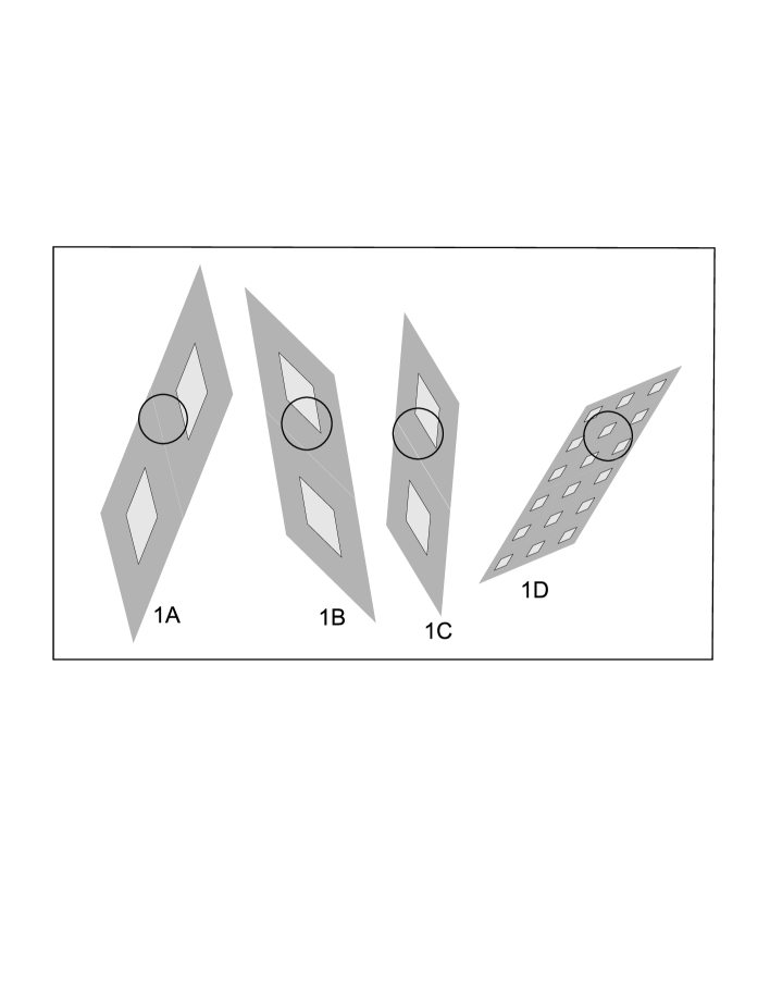
Figure 8: Evolution circle projected on the home sheet $\mathcal{D}_{00}$ for different initial data gathered in Table 1 .

The algorithm described in Section 4 to follow the path on the Riemann surface $\mathcal{R}$ has been implemented in Mathematica. For each of the cases 1A–1D the paths on $\mathcal{R}$ are all periodic, and the periods predicted by the algorithm are indicated in the last column of Table 1. In Figure 9 we show the discontinuous path $\gamma(t)$ on the fundamental domain $\tilde{\mathcal{D}}$ for each of these cases.

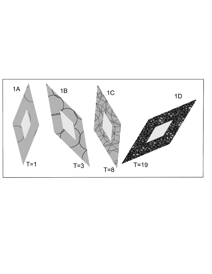
Figure 9: Path $\gamma(t)$ on the fundamental domain for different initial data gathered in Table 1.

The path in Figure 9 is discontinuous because many of the arcs are contained in other sheets $\mathcal{D}_{ij}$ of $\mathcal{R}$. Let us consider a sequence of elements of $\mathbb{Z}^{2}$ corresponding to the index of the sheet $\mathcal{D}_{ij}$ visited by the path after every complete turn. For each of the cases 1A–1D of Table 1 this sequence is depicted in the first column of Figure 10. Note that the sequence in $\mathbb{Z}^{2}$ is periodic if and only if the orbit of the systems of ODEs (12) is closed.

Finally, we have performed a numerical integration of the equations of motion (12) for each of the initial data in Table 1, using an embedded Runge-Kutta method of order 5(4) with automatic step size control, developed by Prince and Dormand in 1981. The results of the integration show periodic orbits whose periods are in perfect agreement with those predicted by the algorithm of Section 4. On the right column of Figure 10 we have displayed the orbits of the function $\zeta(t)$ whose evolution is described by (9) and is trivially related to $z(t)=x(t)+{\rm i}y(t)$ by (5).

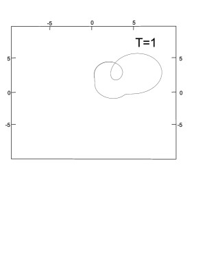
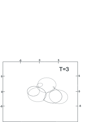
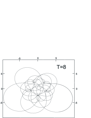
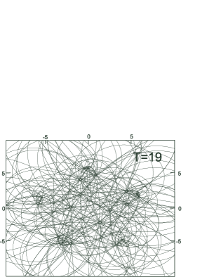
Figure 10: Left column: sequences of sheets of $\mathcal{R}$ visited every complete turn. Right column: orbits of $\zeta(t)$ obtained by numerical integration of the system (9) with $k=4$ for different initial data gathered in Table 1.

5.2 Results for $k=5$

We study now trajectories of the dynamical system (14) corresponding to different initial data. As mentioned in Remark 3.1, this dynamical system describes circular travelling on a Riemann surface $\mathcal{R}$ with only two sheets. Therefore almost all solutions of (14) are periodic with period either $T$ or $2T$. This prediction is confirmed by the numerical integration of the system and some examples of orbits for different initial data have been gathered in Table 2. In all four cases $2A$–$2D$ the initial velocities $\dot{x}(0)=\dot{y}(0)=0$, while the initial positions $\{x(0),y(0)\}$ are displayed in Table 2. For simplicity we have also set $\omega=2\pi$ so that the fundamental period $T=1$.

Table 2: Different sets of initial data for $k=5$

Case	Initial data $(x_{0},y_{0})$	$|E|$	Period
2A	$(1.8,1.9)$	$3.350\cdot 10^{2}$	$1$
2B	$(2.8,2.5)$	$2.865\cdot 10^{3}$	$1$
2C	$(4,4.5)$	$4.781\cdot 10^{4}$	$1$
2D	$(5,8)$	$7.052\cdot 10^{5}$	$1$

Although all the orbits $2A$–$2D$ have the same period, a look at Figures 11 and 12 reveals that the complexity of the orbit increases with increasing energy.

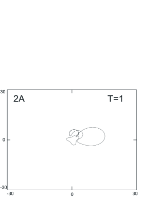
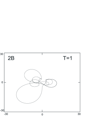
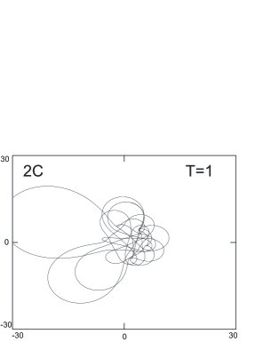
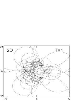
Figure 11: Orbits of $\zeta(t)$ obtained by numerical integration of the system (9) with $k=5$ for different initial data gathered in Table 2.

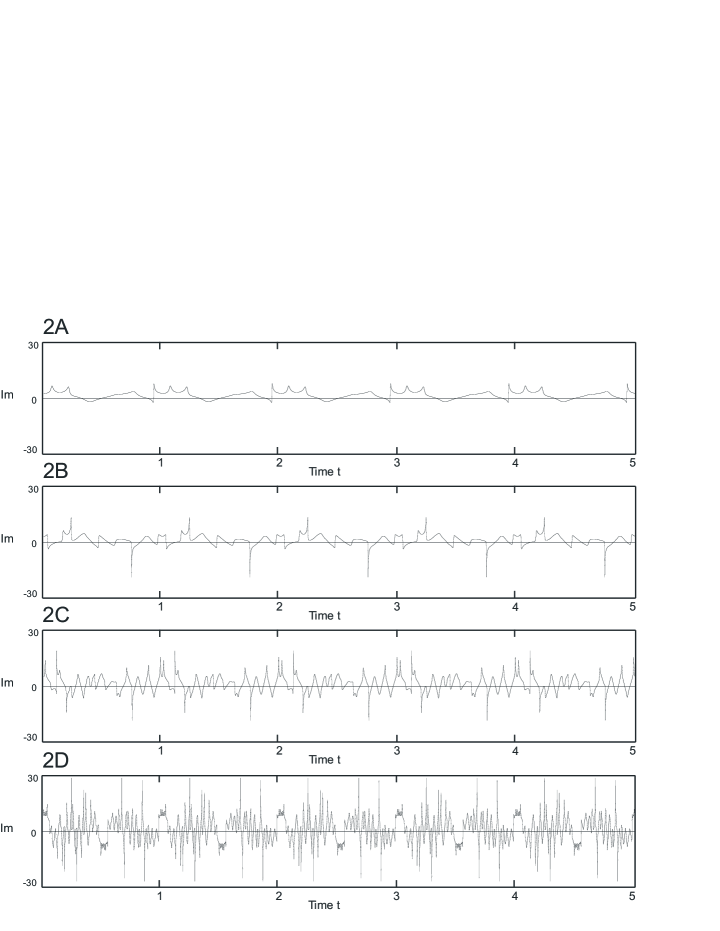
Figure 12: Time evolution of $\textrm{Im}\,\zeta(t)$ obtained by numerical integration of the system (9) with $k=5$ for different initial data gathered in Table 2. All solutions are periodic with the same period $T=1$ but their complexity increases with increasing energy $|E|$.

6 Conclusions

In this paper we introduced a class of dynamical systems on ${\mathbb{R}}^{4}$ whose solutions can be interpreted as lifting a circular path on the complex plane to a generally infititely sheeted Riemann surface $\mathcal{R}$ describing the inversion of a hyperelliptic integral. For the integral of the holomorphic differential $d\eta/\mu$ on a generic genus 2 surface $\Gamma$, we provided an explicit description of the global structure of $\mathcal{R}$ and showed that the surface can be identified with the universal covering of the theta divisor of Jac($\Gamma$). (It should be stressed that in case of another holomorphic differential, in particular $\lambda\,d\lambda/\mu$, the structure of $\mathcal{R}$ and type of branching ${\mathcal{R}}\mapsto{\mathbb{C}}$ are different.) We also noted that for some regular curves with automorphisms, like the sextic curve $\Gamma_{6}$, the four periods of the differential are commensurable, and the corresponding surface $\mathcal{R}$ becomes finitely sheeted. This implies that almost all the trajectories of the corresponding systems are periodic with period $T$ or $2T$, although the trajectories increase in complexity as $|E|$ increases.

Using the global description of $\mathcal{R}$, we provided a geometric algorithm for the circular travelling on $\mathcal{R}$, that replaces the numeric integration of the corresponding ODEs and associates to the path $\gamma(t)$ on $\mathcal{R}$ a sequence on a ${\mathbb{Z}}^{2}$-lattice. We conjecture that for a regular value of the energy, all solutions are periodic, although the periods can be an arbitrarily high integer multiple of the fundamental period.

For didactic reasons we have restricted to genus 2 curves $\Gamma$, although it is also possible to describe the global geometric structure of Riemann surfaces $\mathcal{R}$ for holomorphic integrals on a generic hyperelliptic curve of genus $g>2$. Namely, dividing its $2g$ periods into two allowed and $2g-2$ forbidden ones, one constructs an analog of a $\mathcal{D}$-sheet by removing from $\mathbb{C}$ the union of identical $(4g-4)$-gonal windows $\{{\mathcal{W}}_{ij}\mid i,j\in{\mathbb{Z}}^{2}\}$ which have pairs of parallel edges formed by the forbidden periods. Different windows are obtained from each other by shifts by the allowed periods. Then one can show that the surface $\mathcal{R}$ is itself a union of ${\mathbb{Z}}^{2g-2}$ identical copies of $\mathcal{D}$ glued to each other along the opposite edges of the windows. A trajectory $\gamma(t)$ on $\mathcal{R}$ can be encoded as a path on a ${\mathbb{Z}}^{2g-2}$-lattice.

Acknowledgements

We thank L. Gavrilov, P. Santini, and V. Enolski for discussions and valuable remarks. Our research was partially supported by the Spanish Ministry of Science and Technology under grant BFM 2003-09504-C02-02.

References

- [1] S. Abenda and Yu. Fedorov. On the weak Kowalevski-Painlevé property for hyperelliptically separable systems. Acta Appl. Math., 60(2):137–178, 2000.
- [2] S. Abenda, V. Marinakis, and T. Bountis. On the connection between hyperelliptic separability and Painlevé integrability. J. Phys. A, 34(17):3521–3539, 2001.
- [3] Mark S. Alber and Yuri N. Fedorov. Algebraic geometrical solutions for certain evolution equations and Hamiltonian flows on nonlinear subvarieties of generalized Jacobians. Inverse Problems, 17(4):1017–1042, 2001. Special issue to celebrate Pierre Sabatier’s 65th birthday (Montpellier, 2000).
- [4] Larry Bates and Richard Cushman. Complete integrability beyond liouville-arnold. Rep. Math. Phys., 56(1):77–91, 2005.
- [5] E. D. Belokolos and V. Z. Enolskii. Reduction of abelian functions and algebraically integrable systems. I. J. Math. Sci. (New York), 106(6):3395–3486, 2001. Complex analysis and representation theory, 2.
- [6] E.D. Belokolos, A.I. Bobenko, V.Z. Enol’ski, A.R. Its, and V.B. Matveev. Algebro-Geometric Approach to Nonlinear Integrable Equations. Springer Series in Nonlinear Dynamics. Springer–Verlag, Berlin, 1994.
- [7] C. M. Bender, J.-H. Chen, D. W. Darg, and Milton K. A. Classical trajectories for complex hamiltonians. J. Phys. A, 39:4219–4238, 2006.
- [8] Christina Birkenhake and Herbert Lange. Complex abelian varieties, volume 302 of Grundlehren der Mathematischen Wissenschaften [Fundamental Principles of Mathematical Sciences]. Springer-Verlag, Berlin, second edition, 2004.
- [9] Oskar Bolza. On Binary Sextics with Linear Transformations into Themselves. Amer. J. Math., 10(1):47–70, 1887.
- [10] T. Bountis, L. Drossos, and I. C. Percival. Nonintegrable systems with algebraic singularities in complex time. J. Phys. A, 24(14):3217–3236, 1991.
- [11] F. Calogero and J.-P. Françoise. Periodic motions galore: how to modify nonlinear evolution equations so that they feature a lot of periodic solutions. J. Nonlinear Math. Phys., 9(1):99–125, 2002.
- [12] F. Calogero and J.-P. Françoise. Periodic motions galore: how to modify nonlinear evolution equations so that they feature a lot of periodic solutions. J. Nonlinear Math. Phys., 9(1):99–125, 2002.
- [13] F. Calogero, J.-P. Françoise, and M. Sommacal. Periodic solutions of a many-rotator problem in the plane. II. Analysis of various motions. J. Nonlinear Math. Phys., 10(2):157–214, 2003.
- [14] F. Calogero, D. Gómez-Ullate, P. M. Santini, and M. Sommacal. The transition from regular to irregular motions, explained as travel on Riemann surfaces. J. Phys. A, 38(41):8873–8896, 2005.
- [15] F. Calogero and M. Sommacal. Periodic solutions of a system of complex ODEs. II. Higher periods. J. Nonlinear Math. Phys., 9(4):483–516, 2002.
- [16] Y. F. Chang and G. Corliss. Ratio-like and recurrence relation tests for convergence of series. J. Inst. Math. Appl., 25(4):349–359, 1980.
- [17] Y. F. Chang, J. M. Greene, M. Tabor, and J. Weiss. The analytic structure of dynamical systems and self-similar natural boundaries. Phys. D, 8(1-2):183–207, 1983.
- [18] Y. F. Chang, M. Tabor, and J. Weiss. Analytic structure of the Hénon-Heiles Hamiltonian in integrable and nonintegrable regimes. J. Math. Phys., 23(4):531–538, 1982.
- [19] V. Z. Enolskii, M. Pronine, and P. H. Richter. Double pendulum and -divisor. J. Nonlinear Sci., 13(2):157–174, 2003.
- [20] H. Flaschka. A remark on integrable Hamiltonian systems. Phys. Lett. A, 131(9):505–508, 1988.
- [21] A. S. Fokas and T. Bountis. Order and the ubiquitous occurrence of chaos. Phys. A, 228(1-4):236–244, 1996.
- [22] B. Gambier. Sur les équations différentielles du second ordre et du premier degré dont l intégrale générale est à points critiques fixes. Acta Mathematica, 33:1–55, 1910.
- [23] S. Kowalewskaya. Sur le problème de la rotation d’un corps solide autour d’un point fixe. Acta Mathematica, 12:177–232, 1889.
- [24] S. Kowalewskaya. Sur une propriété du système d’équations différentielles qui définit la rotation d’un corps solide autour d’un point fixe. Acta Mathematica, 14:81–93, 1890.
- [25] M. D. Kruskal, A. Ramani, and B. Grammaticos. Singularity analysis and its relation to complete, partial and nonintegrability. In Partially integrable evolution equations in physics (Les Houches, 1989), volume 310 of NATO Adv. Sci. Inst. Ser. C Math. Phys. Sci., pages 321–372. Kluwer Acad. Publ., Dordrecht, 1990.
- [26] G. Levine and M. Tabor. Integrating the nonintegrable: analytic structure of the Lorenz system revisited. Phys. D, 33(1-3):189–210, 1988. Progress in chaotic dynamics.
- [27] A. I. Markushevich. Introduction to the classical theory of abelian functions, volume 96 of Translations of Mathematical Monographs. American Mathematical Society, Providence, RI, 1992. Translated from the 1979 Russian original by G. Bluher.
- [28] S. P. Novikov. Topology of the generic hamiltonian foliations on the riemann surface. arXiv:math.GT/0505342.
- [29] P. Painlevé. Mémoire sue les équations différentielles du premier ordre. Acta Mathematica, 14:81–93, 1890.
- [30] Ramani, A., Dorizzi, B. and Grammaticos, B.: Painlevé conjecture revisited, Phys. Rev. Lett. 49(21) (1982), 1539 1541.
- [31] A. Ramani, B. Grammaticos, and T. Bountis. The Painlevé property and singularity analysis of integrable and nonintegrable systems. Phys. Rep., 180(3):159–245, 1989.
- [32] M. Tabor and J. Weiss. Analytic structure of the lorenz system. Phys. Rev. A, 24(4):2157–2167, 1981.
- [33] Pol Vanhaecke. Integrable systems and symmetric products of curves. Math. Z., 227(1):93–127, 1998.