Phase lock and rotational motion of a parametric pendulum in noisy and chaotic conditions

Abstract

The effect of noise on a rotational mode of a pendulum excited kinematically in vertical direction has been analyzed. We have shown that for a weak noise transitions from oscillations to rotations and vice versa are possible. For a moderate noise level dynamics of the system is governed by a combination of the excitation amplitude and stochastic component. Consequently for stronger noise the rotational solution as an independent sychonized mode has vanished.
Keywords: Chaotic vibration, rotational mode, noise

1 Introduction

A forced pendulum is one of the simplest nonlinear system which shows typical chaotic behaviour and this has been discussed extensively in many research articles and in several textbooks, for example see [1, 2, 3, 4, 5, 6, 7, 8, 9, 10, 11]. It is worth noting the pendula have been studied not only to understand the fundamental nonlinear behaviour but also with a view to solve some practical problems of wave energy extraction from sea waves [12], gravitational gradient pendulum [13, 14] and ship dynamics [15], to name a few. Some other nonlinear phenomena like the Josephson junction [16, 17] and can also be easily associated with the analysed problem.

In this note we will examine stability of rotational motion of parametric pendulum [6, 11] in noisy conditions [18]. For a pendulum under the harmonic kinematic excitation (Fig. 1a) the equation of motion can be written as follows

$$\frac{{\rm d}^{2}\phi}{{\rm d}t^{2}}+\frac{k}{ml^{2}}\frac{{\rm d}\phi}{{\rm d}t}+\left(\frac{g}{l}+\frac{A}{l}\Omega^{\prime 2}\cos{\Omega^{\prime}t}\right)\sin\phi=0,$$ (1)

where $m$ is point mass $l$ is a length of pendulum, $g$ is a gravitational constant. Introducing the natural frequency of free oscillations, $\omega_{0}=\sqrt{g/l}$ we define dimensionless time $\tau=\omega_{0}t$ and renormalized frequency $\Omega$ $\Omega=\Omega^{\prime}/\omega_{0}$.

(a)

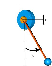
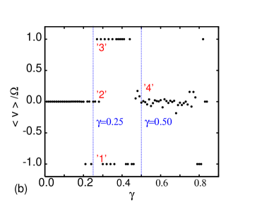
Figure 1: (a) A parametric pendulum with harmonic vertical excitation of a suspension point $x=A\cos\Omega^{\prime}t=A\cos\Omega\tau$, (b) Rotational number $<v>/\Omega$ versus $\gamma$ for $\alpha=0.1$ ($v=\dot{\phi}$). Vertical lines correspond to $\gamma=0.25$ and 0.50 ($\Omega=2$), respectively. Calculations have been done starting from the smallest $\gamma\approx 0$ and increasing it up to $\gamma=0.9$. For each new $\gamma$ the initial conditions $\phi_{0}$ and $v_{0}$ were defined by the final values of $\phi$ and $v$ for previous $\gamma$. Numbers: ’1’, ’2’, ’3’ and ’4’ are related to synchronized motions: clockwise rotation, oscillation, anti-clockwise rotation and chaotic motion, respectively.

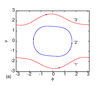
Figure 2: Phase portraits and Poincare maps of the pendulum (Eq. 2) computed for $\omega=2$ $\gamma=0.25$ and $\gamma=0.50$. In Fig. 2a numbers ’1’, ’2’ and ’3’ correspond to solutions marked in Fig. 1b ($\Omega=2$).

Figure 3: Rotation number $<v>/\Omega$ ($\Omega=2$) versus noise level $\sigma$ for $\alpha=0.1$ and four values of $\gamma$; (a) $\gamma=0.4$, (b) $\gamma=0.6$, (c) $\gamma=0.8$, (d) $\gamma=1.0$.

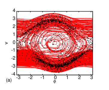
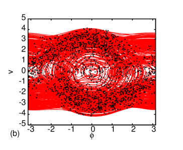
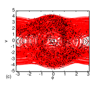
Figure 4: Phase portraits and Poincare maps for $\alpha=0.1$, $\sigma=0.05$ and four values of $\gamma$; (a) $\gamma=0.4$, (b) $\gamma=0.6$, (c) $\gamma=0.8$, (d) $\gamma=1.0$. Note different scales in $v$-axis.

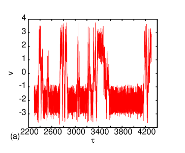
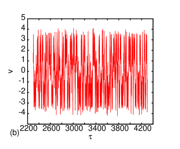
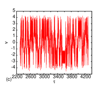
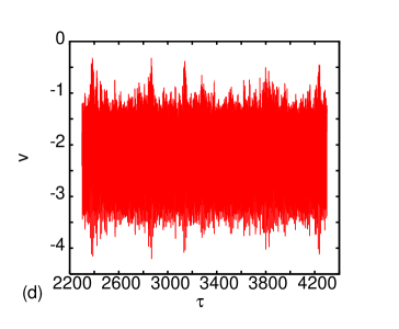
Figure 5: Time series showing the influence of the excitation strength, $\gamma$, computed for $\alpha=0.1$, $\sigma=0.05$, $\Omega=2$; (a)$\gamma=0.4$, (b)$\gamma=0.6$, (c)$\gamma=0.8$, (d)$\gamma=1.0$. Note different scales in $v$-axis.

Figure 6: Rotational number $<v>/\Omega$ ($\Omega=2$) versus $\gamma$ for $\alpha=0.1$ and two different noise levels; (a) $\sigma=0.01$, (b) $\sigma=0.1$.

Note the time dependent term $\frac{A\Omega^{2}}{l}\cos{\Omega\tau}\sin\phi$ is directly related to the inertial force due to the kinematic harmonic excitation with $\Omega^{\prime}$ frequency (Fig. 1a).

$$x(t)=A\cos\Omega^{\prime}t=A\cos\Omega\tau.$$ (2)

To simplify the notation and further analysis we also introduced two new parameters $\gamma=A/l$ and $\beta=k/(ml^{2})$ while time derivative ${\rm d}/{\rm d}\tau\equiv\dot{}$

$$\ddot{\phi}+\beta\dot{\phi}+(1+\gamma\Omega^{2}\cos{\Omega\tau})\sin\phi=0.$$ (3)

Deterministic system regular oscillatory and rotational motions as well as chaotic oscillations can be easily classified by observing changes in so called rotational number $<v>/\Omega$ defined in [1, 19] as

$$<v>/\Omega=\lim_{\tau_{2}\rightarrow\infty}\frac{1}{\Omega(\tau_{2}-\tau_{1})}\int_{\tau_{1}}^{\tau_{2}}\dot{\phi}~{}{\rm d}\tau,$$ (4)

where $\tau_{1}$ was the time interval necessary for the system to reach a steady state (here $\tau_{1}=2.3\times 10^{3}$) while $\tau_{2}$ was chosen to be large enough ($\tau_{2}=4.3\times 10^{3}$). In Fig. 1b we show that this quantity versus $\gamma$ and one can clearly see the regions of synchronized motions and their transitions into chaotic oscillations. Note for the synchronized motion the averaged rotational velocity is kept constant against $\gamma$ parameter up to $\gamma\approx 0.47$ where we observe different behaviour (Fig. 1b). Namely $<v>/\Omega=\pm 1$ for rotations and 0 for an oscillatory motion. The rational number of $<v>/\Omega$ exhibits the phase lock phenomenon [1] characteristic for nonlinear systems. The simulations of deterministic equation (Eq. 2) show that in the relatively large region of system parameters the average velocity is constant. Consequently pendulum motion can be decoupled into two modes: rotations with the average rotational velocity and superimposed oscillations. To illustrate changes in corresponding attractors we plotted (in Fig. 2a and b) phase portraits for $\gamma=0.25$ (and various initial conditions) and $\gamma=0.5$ representing different types of motions.

In the next section we will examine the effect of noise in the examined system (Eq. 3). In particular, we will discuss the simulation results of the rotational number in chaotic and noisy conditions, focusing on destabilization of rotational motions.

2 Phase lock in presence of noise

To examine the system further we have transformed the second order differential equation into two equations of the first order

$$\dot{\phi} = v$$ (5)

$$\dot{v} = -\beta\dot{\phi}-(1+\gamma\Omega^{2}\cos{\Omega\tau})\sin\phi.$$

We assumed that in the system effected by noise through a kinematic excitation is not perfectly periodic resulting in variations of forcing frequency $\Omega^{\prime}$ or its related period $2\pi/\Omega^{\prime}$ in time. Having this in mind we decided to mimic this effect by a bounded noise concept [20] This type of noise is introduced by a random phase to kinematic forcing term $\cos{(\Omega\tau+\Psi)}$, there $\Psi=\Psi(\tau)$ is a Wiener process. To perform numerical calculations we have to discretise our system (Eq. 3). First we write the Euler-Maruyama scheme of integration [21]

$$v_{n+1} = \left(-\beta v_{n}-(1+\gamma\Omega^{2}\cos{\Theta_{n}})\sin\phi_{n}\right)\Delta\tau$$

$$\phi_{n+1} = v_{n}\Delta\tau$$ (6)

$$\Theta_{n+1} = \Theta_{n}+\Omega\Delta\tau+\Gamma(\tau,\sigma)\sqrt{\Delta\tau},$$

where $\Gamma(\tau)$ is a random number with a normal distribution and the standard deviation $\sigma$ referred here as the level of noise. To improve precision of our numerical calculations we have used the Runge-Kutta-Maruyama algorithm

[21] which treats more carefully the deterministic part of Eq. 6. Figures 3a–d show the rotational numbers $<v>/\Omega$ versus $\sigma$ for different $\gamma$. Note that in all cases rotational motion is destructed by noise, and large enough $\sigma$ the resulting cases have variable average velocity. In Fig. 3b the deterministic state is originally chaotic for deterministic case and hence does not change in noisy conditions. Namely the result correspond to the chaotic oscillations with a noise component. For better clarity we have also plotted the phase portraits and Poincare maps for one the chosen value of $\sigma=0.5$ and the same values of $\gamma$ ($\gamma=0.4$, 0.6, 0.8, and 1.0 for Fig. 4a–d respectively). Note, first three figures (Fig. 4a–c) show the system with large amplitude variations but not synchronized rotations; this appears to be chaotic oscillations without any clear synchronized rotation $<v>/\Omega\approx 0$. On the other hand Fig. 4d is representing clock-wise rotations with the fixed average $<v>/\Omega=-1$. The corresponding time series are presented in Figs. 5a–d. Phase lock phenomenon is present in Fig. 5d where we observe anti-clockwise rotation (persistent negative velocity sign). Surprisingly the succeeding Poincare points are smeared by random excitations leaving average velocity $<v>/\Omega=-1$ unchanged. In Fig. 5a, one can see intermittent rotation with a negative sign. Note that in this case for $\sigma=0$ the system behaves regularly (Fig. 3a) with clear clockwise or anti-clockwise rotations ( $<v>/\Omega=\pm 1$). Consequently one can identify a path to chaotic oscillations induced by noise. Finally, in Figs. 6a and b we show $<v>/\Omega$ versus $\gamma$ for two different levels of noise; $\sigma=0.01$ for Fig. 6a and $\sigma=0.1$ for Fig. 6b, respectively. For $\sigma=0.01$ (Fig. 6a) we observe a similar sequence of transitions from oscillatory to rotational motions as in the deterministic case (Fig. 1b), while the noise level, $\sigma=0.1$, as shown in Fig. 6b, is strong enough to destroy the synchronized rotations for any $\gamma$.

3 Summary and Conclusions

We have performed numerical analysis of a parametrically excited pendulum focussing on the rotational motion and the influence of noise in the chaotic regimes. The rotational motion has been computed for the pure deterministic system and for the case with weak bounded noise introduced through a random phase in the excitation term. We found out, that in a large interval of increasing noise level the average rotational velocity was stable; the noise component created oscillations around the rotational average velocity. However, for a large enough noise level $\sigma=0.1$ (Fig. 6a) the rotational motion as an independent sychonized mode has vanished.

Looking for a rotational motion of pendulum we observed an intermittent transition to chaotic motion induced by noise. Such a conclusion was also given by Blackburn in his recent paper [18] where the effect of potential well escape was analyzed assuming a random external force. In our case motivated by a possibility of sea wave energy extraction by a parametric pendulum device, we considered stochastic distribution of the wave phase in succeeding periods.

References

- [1] G.L. Baker, J.P. Gollub, Chaotic dynamics: an Introduction, Cambridge University Press, Cambridge 1996.
- [2] B.S. Bardin and A.P. Markeyev, The stability of the equilibrium of a pendulum for vertical oscillations of the point of suspension, J. Appl. Maths Mechs 59, 879–886 (1995).
- [3] F.C. Moon and P.J. Holmes, A magetoelastic strange attractor, Journal of Sound and Vibration 65, 275–296 (1979).
- [4] W. Szemplinska-Stupnicka, E. Tyrkiel, A. Zubrzycki, The global bifurcations that lead to transient tumbling chaos in a parametrically driven pendulum, Int. J. Bif. Chaos 10, 2161–2175 (2000).
- [5] S.R. Bishop and M.J. Clifford Zones of chaotic behaviour in the parametrically excited pendulum, J. Sound Vibr. 189, 142–147 (1996)
- [6] Szemplinska-Stupnicka W, Tyrkiel E, The oscillation–rotation attractors in the forced pendulum and their peculiar properties Int. J. Bif. Chaos 12 159–168 (2002).
- [7] A. Steindl, H. Troger, Chaotic Motion in Mechanical and Engineering Systems, in Engineering Applications of Dynamics of Chaos, (Eds. W. Szemplińska-Stupnicka, H. Troger) Springer, Wien 1991, pp. 150-223.
- [8] R.W. Leven, B.P. Koch, Chaotic behaviour of a parametrically excited damped pendulum, Phys. Lett. A 86, 71- 74 (1981).
- [9] H.J.T Smith, J.A. Blackburn, Multiperiodic orbits in a pendulum with vertically oscillating pivot, Phys. Rev. E 50, 539 -545 (1994).
- [10] G. Litak, G. Spuz–Szpos, K. Szabelski, J. Warmiński, Vibration of Externally Forced Froude Pendulum, Int. J. Bifurcation and Chaos 9 561–570 (1999).
- [11] X. Xu, M. Wiercigroch, M.P. Cartmell, Rotating orbits of a parametrically-excited pendulum, Chaos, Solitons & Fract. 23, 1537–1548 (2005).
- [12] X. Xu, Nonlinear dynamics of parametric pendulum for wave energy extraction PhD thesis, University of Aberdeen, (2006).
- [13] B.H. Suits, Long pendulums in gravitational gradients, Eur. J. Phys. 27 L7 -L11 (2006).
- [14] S.W. Ziegler and M.P. Cartmell, Using motorized tethers for payload orbital transfer Journal of Spacecraft and Rochets 38 904–913 (2001).
- [15] J. Falzarano, A. Steindl, A. Troesch, and H. Troger. Rolling Motion of Ships Treated as Bifurcation Problem. In R. Seydel, et al., editor, Bifurcation and Chaos: Analysis, Algorithms, Applications, volume 97 of ISNM, pp. 117–122. Birkhaeuser-Verlag, Basel, 1991.
- [16] G. Cicogna, A theoretical prediction of the threshold for chaos in a Josephson junction, Physics Lett. A 121, 403–406 (1987).
- [17] S.H. Strogatz, Nonlinear Dynamics and Chaos, Perseus Books Publishing, Cambridge MA 1994.
- [18] J.A. Blackburn, Noise activated transitions among periodic states of a pendulum with a verticaly oscillationg pivot, mediated by a chaotic attractor, Proc. R. Soc. A 462, 1043–1052 (2006).
- [19] E.A. Kim, K.C. Lee, M.Y. Choi, S. Kim, Rotational number approach to a damped pendulum under parametric forcing, J. Korean Phys. Soc. 44, 518–522 (2004).
- [20] W.Y. Liu, W.Q. Zhu, Z.L. Huang, Effect of bounded noise on chaotic motion of Duffng oscillator under parametric excitation, Chaos, Solitons & Fractals 12, 527–537 (2001).
- [21] A. Naess, V. Moe, Efficient path integration method for nonlinear dynamic systems, Probalistic Engineering Mechanics 15, 221- 231 (2000).