Spot deformation and replication in the two-dimensional Belousov-Zhabotinski reaction in water-in-oil microemulsion

Abstract

In the limit of large diffusivity ratio, spot-like solutions in the two-dimensional Belousov-Zhabotinski reaction in water-in-oil microemulsion are studied. It is shown analytically that such spots undergo an instability as the diffusivity ratio is decreased. An instability threshold is derived. For spots of small radius, it is shown that this instability leads to a spot splitting into precisely two spots. For larger spots, it leads to deformation, fingering patterns and space-filling curves. Numerical simulations are shown to be in close agreement with the analytical predictions.

Localized patterns such as spots belong to the class of dissipative structures found far from equilibrium DStruc . In recent years, considerable progress has been made in the understanding of these systems. The question of stability of such patterns is central and the source of instabilities must be carefully scrutinized. In particular, the occurrence of instability can lead to the deformation of spots followed by spot multiplication (also called self-replication) or fingering. This intriguing phenomenon has been the subject of research since the pioneering work of Pearson pearson . Shortly after, thanks to the development of open spatial chemical reactors, self-replication was observed in various experiments such as ferrocyanide-iodate-sulphite reaction lmps , the Belousov-Zhabotinsky reaction mpm ; kve ; kve2 , and chloride dioxide-malonic-acid reaction DBDK . By now this phenomenon is believed to be universal mo ; hayase1 . It is not restricted to chemical reactions and occurs in many systems in biology meron , material science RW ; ns and nonlinear optics laser .

Analytically, spot replication is relatively well understood in one dimensional setting. Nishiura and Ueyama N5 proposed that self-replication of spikes occurs when the spike solution dissapears due to the presence of a fold point. Similar explanation has been reported for the box-like patterns OK . In two dimensions, a mechanism for spot instability has been proposed in mo for general reaction-diffusion systems; related analysis was performed earlier in the framework of a piecewise-linear approximation in omk , km and more recently in the context of diblock copolymer systems RW , ns . See also Goldstein , Mmotion and gcom and for a related approach from the point of view of interface motion.

In this letter we perform an analytical and numerical investigation of the two-dimensional localized spots that were recently reported for the Belousov-Zhabotinski (BZ) reaction in water-in-oil microemulsion kve , kve2 . In the classical BZ reaction, spiral waves are observed KT but no localized spot solutions are possible. Indeed, localized structures develop only when the ratio of diffusion coefficients is sufficiently large, which occurs in the microemulsion system but not in the classical BZ reaction.

We consider the water-in-oil microemulsion model of the BZ reaction as described in kve and kve2 :

$$\begin{aligned} \varepsilon_{0}v_{t}=\varepsilon_{0}D_{v}\Delta v+\left[f_{0}z+i_{0}\left(1-mz\right)\right]\frac{v-q_{0}}{v+q_{0}}\\ +\left[\frac{1-mz}{1-mz+\varepsilon_{1}}\right]v-v^{2}\end{aligned}$$ (1a)

$$z_{t}=D_{z}\Delta z-z+v\left[\frac{1-mz}{1-mz+\varepsilon_{1}}\right]$$ (1b)

where $v,z$ are dimensionless concentrations of activator HBrO₂ and oxidized catalyst $[Ru(bpy)_{3}]^{3+}$ respectively; $D_{v}$ and $D_{z}$ are dimensionless diffusion coefficients of activator and catalyst; $f,\varepsilon$ and $q$ are parameters of the standard Keener-Tyson model KT ; $i_{0}$ represents the photoinduced production of inhibitor, and $m$ represents the strength of oxidized state of the catalyst with $0<mz<1$. This reaction was shown experimentally and numerically to admit localized spot patterns that persist for long time kve , kve2 .

We rescale the variables as $z=1/m-m^{-3/2}w\varepsilon_{1},~{}~{}v=m^{-1/2}\hat{v},~{}~{}t=\varepsilon_{0}m^{1/2}\hat{t}.$ In the new variables, after dropping the hats, we obtain

$$v_{t}=\varepsilon^{2}\Delta v+f(v,w);\ \ \tau w_{t}=D\Delta w+g(v,w)$$ (2a)

where

$$f(v,z) =-\left[f_{0}+f_{1}w\right]\frac{v-q}{v+q}+\left[\frac{w}{1+\alpha w}\right]v-v^{2};$$ (2b)

$$g(v,w) =1-\left[\frac{w}{1+\alpha w}\right]v$$ (2c)

and with the nondimensional constants given by

$$\begin{aligned} &\alpha=m^{-1/2},~{}~{}f_{1}=\varepsilon_{1}m^{1/2}\left(i_{0}-\frac{f_{0}}{m}\right),~{}~{}q=q_{0}m^{1/2},\\ &\varepsilon^{2}=\varepsilon_{0}D_{v}m^{1/2},~{}~{}D=D_{z}\varepsilon_{1}m^{-1/2},~{}~{}\tau=\frac{1}{m}\frac{\varepsilon_{1}}{\varepsilon_{0}}.\end{aligned}$$ (3)

In the limit $m\rightarrow\infty,\ f_{1}\rightarrow 0$ and $\tau\rightarrow 0\ \$we obtain the reduced system,

$$\left\{\begin{aligned} v_{t}&=\varepsilon^{2}\Delta v-f_{0}\frac{v-q}{v+q}+wv-v^{2}\\ 0&=D\Delta w+1-vw.\end{aligned}\right.$$ (4)

In particular, parameter values used in Fig. 14 of kve2 are $f_{0}=2.18,i_{0}=0,m=10,\varepsilon_{1}=0.01,\varepsilon_{0}=0.1$ and $D_{z}/D_{v}=100$ which gives $\alpha=0.3,f_{1}=-0.007,\tau=0.01$, so that the simplification (4) is appropriate.

(a)

(b)                         (c)

Figure 1: (a) Radially symmetric, stable spot solution of the reduced BZ system (4) in the BZ system on a unit disk. (b) Radial profile of $v$ (solid curve) and its asymptotic approximation (dashed curves) given by (7). Insert: a blowup showing the profile of the interface. (c) Radial profile of $w$ (solid curve) and its two-term asympotic approximations (dashed curves) given by (10). Parameter values are $D=20,f_{0}=2.0,\varepsilon=0.02,q=0.005.$

Experimental and numerical evidence in kve and kve2 suggest that (1) admits localized spot soltuions, such as shown in Fig. 1. Such spots occur in the regime where $\varepsilon\ll 1.$ Our goal is to describe analytically the radius and profile of such a spot and then study its stability using singular perturbation techniques similar to those described in mo . As we will demonstrate, the instability thresholds appear in the regime where $D\gg 1$. For sufficiently large values of $D$ a spot pattern is stable. However as $D$ is decreased, instabilities of the form $\exp(\lambda t)\cos(m\theta)\phi(r)$ may develop, where $\theta$ and $r$ are the angular and radial coordinates, respectively. We provide the analytic description of the profile of the spot (7, 10) and the dispersion relation (14) between $m$ and $\lambda$. This relation leads directly to the estimate for the instability threshold.

We begin by constructing a stationary (time-independent) spot-type solution on a two dimensional unit disk $\left\{x:\left|x\right|<1\right\}$. We assume that $D\gg 1$. Then to leading order, $w\sim w_{0}$ is a constant to be determined, and the solution for $v$ consists of an interface located at $\left|x\right|\sim l$ which connects two nearly spatially homogeneous layers. To find the profile of such an interface and its location $l$, let us rescale near $l$ as $v\left(x\right)=V\left(y\right)$ with $y=\left(r-l\right)/\varepsilon$ and $r=\left|x\right|.$ For the steady state we then obtain, to leading order, $V^{\prime\prime}\left(y\right)+f\left(V;w_{0}\right)=0.$ The interface solution corresponds to a heteroclinic orbit of this ODE. The existence of such an orbit is only possible whenever the equations

$$f\left(V_{-};z_{0}\right)=0=f\left(V_{+};w_{0}\right),\ \ \ \ \int_{V_{-}}^{V_{+}}f\left(s;w_{0}\right)ds=0$$ (5)

are simultaneously satisfied for some values $V_{-}$ $<V_{+}.$ Since $q\ll 1$, we have $V_{-}\sim 0$ and (5) can be written as

$$f_{0}+f_{1}w_{0}\sim\frac{3}{16}\left[\frac{w_{0}}{1+\alpha w_{0}}\right]^{2};\ \ \ V_{+}\sim\frac{3}{4}\left[\frac{w_{0}}{1+\alpha w_{0}}\right].$$ (6)

Next, we ignore the $O(q)$ terms and integrate $V^{\prime\prime}(y)+f(V,w_{0})=0$ to obtain

$$v \sim\left\{\begin{aligned} &V_{+}\tanh^{2}\left(\sqrt{\frac{V_{+}}{6}}\left(\dfrac{r-l}{\varepsilon}\right)\right),~{}~{}&r<l\\ &0,&r>0\end{aligned}\right.$$ (7)

with $V_{+}$ and $w_{0}$ given by (6) and where $r=\left|x\right|$. This formula describes the profile of the interface in the limit $q\to 0$. Its thickness is of $O(\varepsilon V_{+}^{-1/2}).$ To determine its location $l$, we integrate the second equation in (2a). Zero-flux conditions then yield $\int g=0$ so that

$$g\left(V_{+},w_{0}\right)l^{2}+\left(1-l^{2}\right)g\left(0,w_{0}\right)\sim 0$$ (8)

In the limit of the reduced system (4), we obtain

$$l\sim\frac{1}{2\sqrt{f_{0}}},\ \ w_{0}\sim\frac{4}{\sqrt{3}}\sqrt{f_{0}},\ \ \ V_{+}\sim\sqrt{3f_{0}}.$$ (9)

To determine the correction to $w,$ we write $w=w_{0}+D^{-1}w_{1}+O\left(D^{-2}\right)$. to obtain $\Delta w_{1}+g\left(w_{0},v_{0}\right)=0.$ Imposing continuity at the interface $r=l$, the solvability condition $w_{1}(l)=0$, and using (8) and $g\left(0,w_{0}\right)=1,$ we then obtain

$$w\sim w_{0}+\frac{1}{4D}\left\{\begin{aligned} &-\dfrac{(1-l^{2})(l^{2}-r^{2})}{l^{2}},&r<l\\ &2\ln(\dfrac{r}{l})+l^{2}-r^{2},&r>l\end{aligned}\right..$$ (10)

An example of a localized spot and its radial profile are shown in Fig 1.

When decreasing the diffusion coefficient $D$ of the recovery variable, numerical simulations show that the spot becomes unstable. To compute the threshold associated with this instability, we linearlize around the localized spot solution (7) as

$$v(x,t) =v(x)+\exp\left(\lambda t\right)\cos\left(m\theta\right)\phi\left(r\right)$$

$$w(x,t) =w(x)+\exp\left(\lambda t\right)\cos\left(m\theta\right)\psi\left(r\right)$$

where $v$ and $w$ are given to leading order in (7 and 9) spot-type solution, $m$ is an integer, $\phi,\psi\ll 1$ and $(r,\theta)$ are the polar coordinates of $x.$ Substituting into (1) we then obtain

$$\lambda\phi =\varepsilon^{2}\left(\phi_{rr}+\frac{1}{r}\phi_{r}-\frac{m^{2}}{r^{2}}\phi\right)+f_{v}\phi+f_{w}\psi$$ (11a)

$$\tau\lambda\psi =D\left(\psi_{rr}+\frac{1}{r}\psi_{r}-\frac{m^{2}}{r^{2}}\psi\right)+g_{v}\phi+g_{w}\psi.$$ (11b)

Note that $v_{r}$ satsifies that $\varepsilon^{2}(v_{rrr}+1/rv_{rr}-1/r^{2}v_{r})+f_{v}v_{r}+w_{r}f_{w}=0.$ Therefore multiplying (11b) by $v_{r}$ and integrating by parts, we obtain

$$\left(\lambda+\frac{(m^{2}-1)\varepsilon^{2}}{l^{2}}\right)\int v_{r}^{2}\sim\int v_{r}f_{w}\left(\psi-w_{r}\right).$$ (12)

where we have assumed that to leading order, $\phi\sim v_{r},\lambda\ll 1,\psi\ll\phi$. Since $v_{r}$ is exponentially small outside the interface, we simplify $\int v_{r}f_{w}\left(\psi-w_{r}\right)\sim-\left(\psi\left(l\right)-w_{r}\left(l\right)\right)\int_{0}^{V_{+\ }}f_{w}\left(v,w_{0}\right)dv$. We estimate $w_{r}(l)\sim-1/(2D)g\left(V_{+},w_{0}\right)$ and to determine $\psi\left(l\right),$ we integrate (11b) over the interface $l$ to obtain $D\psi_{r}|_{l^{-}}^{l^{+}}\sim-g\left(0,w_{0}\right)/l^{2}$ where we have used $\phi\sim v_{r}$ and (8). Keeping only leading order terms in $D$ we then obtain the following problem for $\psi$:

$$0=\psi_{rr}+\frac{1}{r}\psi_{r}-\frac{m^{2}}{r^{2}}\psi=0,~{}~{}~{}~{}r\neq l$$ (13a)

$$\psi^{\prime}(0)=0=\psi^{\prime}(1),~{}~{}\psi^{\prime}\left(l^{+}\right)-\psi^{\prime}\left(l^{-}\right)=-\frac{1}{Dl^{2}}g\left(0,w_{0}\right).$$ (13b)

Using the continuity of $\psi$ at $r=l$ we get

$$\psi\left(l\right)\sim\frac{1}{2Dml}g\left(0,w_{0}\right)\left(1+l^{2m}\right)$$

and substituting into (12) we obtain

$$\lambda\frac{l^{2}}{\varepsilon^{2}}\sim 1-m^{2}+A\left[1-l^{2}-\frac{1}{m}\left(1+l^{2m}\right)\right]$$ (14)

where

$$A=\frac{l}{2\varepsilon D}\frac{g\left(0,w_{0}\right)\left(\int_{0}^{V_{+\ }}f_{w}\left(v,w_{0}\right)dv\right)}{\varepsilon\int v_{r}^{2}}.$$ (15)

For the reduced model (4) we obtain an explicit result

$$A\sim\frac{3^{5/4}2^{1/2}5}{64}\frac{1}{f_{0}^{3/4}\varepsilon D}=0.43622\frac{1}{f_{0}^{3/4}\varepsilon D}.$$ (16)

In Fig. 2, the analytical prediction given by (14) is found to be in good agreement with the numerical computations of problem (11). Full numerical simulations of (4) also agree with this prediction. For example, when taking $\varepsilon=0.03,f_{0}=1.3$ and $q=0.01$, slight spot deformation corresponding to mode $m=2$ is observed when $D=1.0$ but not when $D=1.3.$ This agrees well with $D\sim 1.1$, the threshold predicted by (14).

Figure 2: (a), (b) Comparison of numerical computations of $\lambda$ given by (11) (diamonds) with the analytical result (14, 16) (dashed line) for the reduced model (4) on a unit disk. Parameter values are $q=0.01$, $\varepsilon=0.01$ and (a) $D=3,f_{0}=1.3$; (b) $m=2,f_{0}=1.3$. (c) Simultaneous solution of $\lambda=0=d\lambda/dm$, showing the first value of $D$ for which instability occurs. The system is stable above the curve and unstable below it. To compute $\lambda$ numerically, (11) was reformulated as a boundary value problem by adjoining the equation $d\lambda/dr=0$ along with fixing $\psi(1).$ Maple’s numerical boundary value problem solver was then used with initial guesses $\phi=v_{r},\lambda=0$ and $\psi=$ the solution of (13). All computations are correct to four significant digits.

From (14) and (16), it is clear that the mode $m=1$ is always stable and that for large enough $D$, all modes $m\geq 1$ are stable. As $D$ is decreased, instability sets in when $D=O(\varepsilon^{-1})$. The threshold value is found by simultaneously solving $\lambda=d\lambda/dm=0$. The resulting graph is shown on Fig. 2c. In particular, note that the system is stable if $D\varepsilon>0.038$, independent of the value of $f_{0}.$ In the limit of small radius $l\rightarrow 0$, the first unstable integer mode is $m=2$ corresponding to $A=6,$ so that the spot of small radius becomes unstable whenever $\varepsilon Df^{3/4}\leq 0.0727.$ More generally, by eliminating $A$ we find that there exist constants $l_{1}<l_{2}<\ldots<1$ such the first unstable mode is $m$ provided that $l_{m-1}<l<l_{m},$ where $l_{1}=0$, $l_{2}=0.491$, $l_{3}=0.667$, $l_{4}=0.753$ and $l_{m}\sim 1-0.937/m$ as $m\rightarrow\infty;$ where 0.937 is the root of $e^{-2z}\left(3+2z\right)+3-4z=0.$

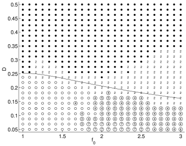
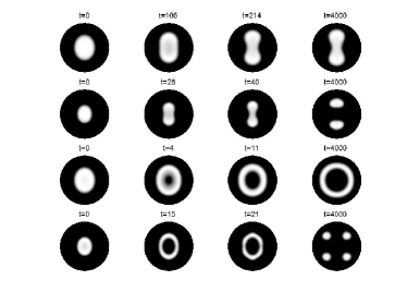
(a)   (b)

Figure 3: (a) Bifurcation diagram for (4) in $D$ and $f_{0}$ with $\varepsilon=0.05,q=0.01.$ Solid dots represent deformations of a spot without topological change. Points marked by ”2” represent spot-replication into two spots. An empty circle represents spot-to-ring bifurcation and empty circle with a number inside represents spot-to-ring-to-spots bifurcation. A solid line represents the boundary of spot-to-ring replication which occurs at the fold point of the radially symmetric steady state. The bifurcation diagram was obtained by solving the full two-dimensional system (4) using the finite element package FlexPDE FlexPDE with zero-flux boundary conditions and 800 elements on a quarter-disk. For initial conditions, (7, 9, 10) was used, but with $r$ replaced by $r(1+0.05\cos 2\theta)$. The solid line was obtained by solving for the fold point of the radially symmetric steady state using Maple’s boundary value problem solver. (b) Full numerical simulations starting from a spot-state (7, 10) as initial conditions. First row: spot deformation, $f_{0}=1.3,D=0.35$. Note that the final stedy state of the system is a deformed blob shown here at $t=4000$. Second row: self-replication, $f_{0}=2.2,D=0.24$. Third row: spot-to-ring bifurcation, $f_{0}=1.3,D=0.1$. Fourth row: spot-to-ring-to-spots bifurcation, $f_{0}=2.6,D=0.1$.

Numerical computations indicate that self-replication is more prevalent for spots of small radius (see Fig. 3). For larger spots, a deformation usually leads to to the so-called ”finger growth” and space filling curves. Others studies have shown the occurrence of fingering instabilities leading to labyrinthine patterns Fingers , Goldstein , mo . The question of whether the self-replication or fingering instability occurs first is still open.

For smaller, $O(1)$ values of $D$, there is also a different instability mechanism that can lead to splitting of a spot into a ring as illustrated in Fig. 3. Unlike spot multiplication, this instability is radially symmetric, and is caused by the dissapearence of the steady state solution – whereby the steady state solution ceases to exist due to the presence of a saddle-node bifurcation – rather than by its lateral instability. Numerical simulations suggest that that spot replication occurs only for spots of smaller radius, whereas spot-to-ring instability is dominant for larger spots.

To conclude, we have estimated analytically for which value of diffusion $D$ spot deformation first occurs. As is $D$ is decreased further, self-replication and/or spot-to-ring instability is observed. As evidenced by numerical simulations, we conjecture that spot deformation is the precursor to this phenomenon.

References

• (1) The authors are grateful to Vladimir Vanag and Irving Epstein for introducing us to this subject and for illuminating discussions. We are also grateful to the anonymous referees whose suggestions have improved the paper significantly. T.K. is supported by NSERC Canada, and the Dalhousie University startup grant. M.T. is supported by the FNRS Belgium.
• (2) P. Glansdorff and I. Prigogine, Thermodynamic Theory of Structures, Stability and Fluctuations (Wiley, New York, 1971); E. Meron, Phys. Rep. 218, 1 (1992); J. Chanu and R. Lefever, Inhomogeneous phases and pattern formation, Physica A 213, 1-276 (1995); M.C. Cross and P.C. Hohenberg, Mod. Phys. Rep. 65, 851 (1993); K. Kapral and K. Showalter, Chemical Waves and Patterns (Kluwer Academic press, Dordercht, 1995).
• (3) J.E. Pearson, Science, 261, 189 (1993).
• (4) K. Lee, W.D. McCormick, J.E. Pearson, and H.L. Swinney, Nature, 396, 215 (1994).
• (5) A.P. Muñuzuri, V. Pérez-Villar, and M. Markus, Phys. Rev. Lett. 79, 1940 (1997).
• (6) A. Kaminaga, V.K. Vanag, and I.R. Epstein, Angewandte Chemie, 45, 3087 (2006).
• (7) A. Kaminaga, V.K. Vanag, and I.R. Epstein, J. Chem. Phys. 122, 174706 (2005).
• (8) P.W. Davis, P. Blanchedeau, E. Dulos, and P. De Kepper, J. Phys. Chem. A 102 8236 (1998).
• (9) C. Muratov and V.V. Osipov, Phys. Rev. E 53, 3101 (1996); Phys. Rev. E 54, 4860 (1996); C. Muratov, Phys. Rev. E 66, 066108 (2002).
• (10) Y. Hayase and T. Ohta, Phys. Rev. Lett. 81, 1726 (1998); Y. Hayase, Phys. Rev. E 62, 5998 (2000).
• (11) E. Meron, E. Gilad J. von Hardenberg, and M. Shachak, Chaos, Solitons and Fractals, 19, 367 (2004).
• (12) X. Ren and J. Wei, SIAM J. Math. Anal. 35, 1 (2003).
• (13) Y.Nishiura and H.Suzuki, SIAM Math.Anal. 36(3), 916 (2004).
• (14) M. Tlidi A.G. Vladimirov, and P. Mandel, Phys. Rev. Lett. 89, 233901 (2002).
• (15) Y. Nishiura and D. Ueyama, Physica D 130, 73 (1999).
• (16) B.S. Kerner and V.V. Osipov, Autosolitons: A new Approach to Problems of Self-Organization and Turbulence (Kluwer, Dordrecht, 1994).
• (17) T. Ohta, M. Mimura, and R. Kobayashi, Physica D 34, 115 (1989).
• (18) S.Kawaguchi and M.Mimura, SIAM J.Appl,Math 59, 920(1999)
• (19) J.J. Tyson and P. Fife, J. Chem. Phys. 73, 2224 (1980); J.P. Keener and J.J. Tyson, Physica D 21, 307 (1986).
• (20) R.E. Golstein, D.J. Muraki, and D.M. Petrich, Phys. Rev. E 53, 3939 (1996).
• (21) C.B. Muratov, Phys. Rev. E 54, 3369 (1996)
• (22) D. Gomila, P. Colet, G.L. Oppo and M. San Miguel, Phys. Rev. Lett. 87, 194101 (2001).
• (23) K. Lee and H. Swinney, Phys. Rev. E 51, 1899 (1995).
• (24) See FlexPDE website, www.pdesolutions.com.